Influence of Stellar Multiplicity On Planet Formation. IV. Adaptive Optics Imaging of Kepler Stars With Multiple Transiting Planet Candidates

Abstract

The Kepler mission provides a wealth of multiple transiting planet systems (MTPS). The formation and evolution of multi-planet systems are likely to be influenced by companion stars given the abundance of multi stellar systems. We study the influence of stellar companions by measuring the stellar multiplicity rate of MTPS. We select 138 bright (K${}_{P}<13.5$) Kepler MTPS and search for stellar companions with AO imaging data and archival radial velocity (RV) data. We obtain new AO images for 73 MTPS. Other MTPS in the sample have archival AO imaging data from the Kepler Community Follow-up Observation Program (CFOP). From these imaging data, we detect 42 stellar companions around 35 host stars. For stellar separation $1\ \rm{AU}<a<100$ AU, the stellar multiplicity rate is $5.2\pm 5.0$% for MTPS, which is 2.8$\sigma$ lower than $21.1\pm 2.8$% for the control sample, i.e., the field stars in the solar neighborhood. We identify two origins for the deficit of stellar companions within 100 AU to MTPS: (1) a suppressive planet formation, and (2) the disruption of orbital coplanarity due to stellar companions. To distinguish between the two origins, we compare the stellar multiplicity rates of MTPS and single transiting planet systems (STPS). However, current data are not sufficient for this purpose. For $100\ \rm{AU}<a<2000$ AU, the stellar multiplicity rates are comparable for MTPS ($8.0\pm 4.0$%), STPS ($6.4\pm 5.8$%), and the control sample ($12.5\pm 2.8$%).

1. Introduction

As exoplanet surveys reach higher sensitivity and longer time baseline, more exoplanets are being discovered. Many of these exoplanets are in multi-planet systems. As of September 2015, the radial velocity (RV) technique and the transit method have detected 152 and 857 planets in multi-planet systems (http://exoplanets.org, Han et al., 2014). From these systems, we can study their orbital spacing (e.g., Wright et al., 2011; Burke et al., 2014), mutual inclination (e.g., Lissauer et al., 2011; Tremaine & Dong, 2012), and eccentricity distribution (e.g., Jurić & Tremaine, 2008; Kane et al., 2012; Xie, 2015). These studies can be used to test theories of planet formation and dynamical evolution (Winn & Fabrycky, 2015).

While only $\sim$20% of Kepler planet host stars are multiple transiting planet systems (MTPS), the total number of planets in MTPS accounts for almost half of the Kepler planet candidates. Latham et al. (2011) compared Kepler MTPS to single transiting planet systems (STPS). They found a lack of gas giant planets in MTPS, which indicates that the existence of a gas giant planet may disrupt the orbital inclinations or suppress the formation of multiple planets. Furthermore, other studies implied that the distributions of orbital spacings (Xie et al., 2014), eccentricities (Xie, 2015) and obliquities (Morton & Winn, 2014) are different for STPS and MTPS. In this paper, we investigate one possibility that causes the different orbital architecture between STPS and MTPS, namely, the influence of dynamically-bound companion stars.

By comparing stellar multiplicity rate for 138 MTPS against stars in the solar neighborhood (Raghavan et al., 2010; Duquennoy & Mayor, 1991), Wang et al. (2014b) found evidence of suppressive planet formation in multiple stellar systems with stellar separations smaller than 20 AU. Beyond 20 AU, the stellar multiplicity rate was difficult to measure without high resolution and deep imaging data that provide sensitivity to stellar companions at these separations. Therefore, at separations wider than 20 AU, the influence of stellar companions on multi-planet formation was not well understood. In this paper, we gather adaptive optics (AO) images for the same MTPS sample in Wang et al. (2014b). Since AO images for 65 MTPS are already available from the Kepler Community Follow-up Observation Program (CFOP), we obtain new AO images for the remaining 73 MTPS at Keck observatory and Palomar observatory. The archival and newly obtained AO images reveal dozens of new stellar companions to planet host stars and put valuable constraints on multi-planet formation in multiple stellar systems.

The paper is organized as follows. We describe the sample selection and AO data acquisition in §2, followed by data analyses in §3. We report the stellar multiplicity rate for MTPS in §4. Discussion and summary are given in §5.

2. Sample Description and AO Data Acquisition

2.1. Sample Description

The sample of MTPS remains the same as that in Wang et al. (2014b). From the NASA Exoplanet Archive, we select Kepler Objects of Interest (KOIs) that satisfy the following criteria: (1), disposition of either Candidate or Confirmed; (2), with at least two planet candidates; (3), Kepler magnitude ($K_{P}$) brighter than 13.5. The above selection criteria resulted in 138 MTPS in Wang et al. (2014b). With the updated Exoplanet Archive, the selection criteria resulted in 208 MTPS. In this paper, we focus on the 138 MTPS to be consistent with previous work. Their stellar and orbital parameters can be found in Table 2 and Table 3 in Wang et al. (2014b).

Most MTPS in our sample are true planetary systems based on a statistical analysis by Lissauer et al. (2012). Subsequent papers on Kepler MTPS validated 851 planet candidates in 340 systems (Rowe et al., 2014; Lissauer et al., 2014), 66 MTPS in our sample are included in those validated systems. Furthermore, 25 additional MTPS in our sample are confirmed planetary systems and the remaining 47 MTPS have disposition of planet candidate according to the latest NASA Exoplanet Archive. Therefore, the false positive rate for the MTPS sample studied in this paper should be extremely low.

2.2. AO Data Acquisition

2.2.1 Archival AO Data For Follow-up Observations

We checked the continually updated CFOP. To avoid repeated AO observations, we only observed KOIs that did not received AO follow-up observations. Some of the KOIs without AO data may have speckle imaging (e.g., Horch et al., 2012, 2014) or lucky imaging data (e.g., Lillo-Box et al., 2012, 2014), but we re-observed these KOIs at Palomar and Keck Observatory because near infrared AO images provide deeper sensitivity and/or higher spatial resolution. For the same reason, we re-observed KOIs that have been observed by the Robo-AO project (Law et al., 2014). For those KOIs whose AO data from Palomar, MMT, or Keck telescope were available through CFOP, we used the archival AO data. In total, AO data for 65 KOIs were obtained from CFOP and AO data for 73 KOIs were obtained by new observations at Palomar and Keck observatory.

2.2.2 AO Imaging with PHARO at Palomar

We observed 68 KOIs in the sample with the PHARO instrument (Brandl et al., 1997; Hayward et al., 2001) at the Palomar 200-inch telescope (San Diego County, California, United States). The observations were made between UT July 13rd and 17th in 2014 with seeing varying between 1.0^′′ and 2.5^′′. PHARO is behind the Palomar-3000 AO system, which provides a on-sky Strehl of 86% in $K$ band (Burruss et al., 2014). The pixel scale of PHARO is 25 mas pixel^-1. With a mosaic 1K $\times$1K detector, the field of view (FOV) is 25${}^{\prime\prime}\times$25^′′. We normally obtained the first image in $K$ band with a 5-point dither pattern, which had a throw of 2.5^′′. AO images in $K$ band provide higher sensitivity to bound companions with late spectral type than $J$ and $H$ band images. Furthermore, the AO correction in $K$ band is better and offers a better characterized point spread function (PSF). This is because image quality improves towards longer wavelength for a given wavefront sensing and correcting error (Davies & Kasper, 2012). A better image with a more stable PSF facilitates companion detection and characterization. Exposure time was set such that the peak flux of the KOI is at least 10,000 ADU for each frame, which is within the linear range of the detector. If a stellar companion was detected, we observed the KOI in $J$ and $H$ bands right after the $K$ band observation. The color information is useful for estimating the stellar properties of the stellar companion and determining whether the companion is physically bound (see §3.2). Nearly simultaneous $J$, $H$, and $K$ band observations help to minimize the influence of any time variability of the target.

2.2.3 AO Imaging with NIRC2 at Keck II

We observed 5 KOIs in the sample with the NIRC2 instrument (Wizinowich et al., 2000) at the Keck II telescope (Mauna Kea, Hawaii, United States). The observations were made on UT July 18th and August 18th in 2014 with excellent/good seeing between 0.3^′′ to 0.8^′′. NIRC2 is a near infrared imager designed for the Keck AO system. We selected the narrow camera mode, which has a pixel scale of 10 mas pixel^-1. The FOV is thus 10${}^{\prime\prime}\times$10^′′ for a mosaic 1K $\times$1K detector. We started the observation in $K$ band for each KOI for the same reason stated in §2.2.2 and followed by $J$ and $H$ band observations if any stellar companions were found. The exposure time setting is the same as the PHARO observation: we ensured that the peak flux is at least 10,000 ADU for each frame. We used a 3-point dither pattern with a throw of 2.5^′′. We avoided the lower left quadrant in the dither pattern because it has a much higher instrumental noise than the other 3 quadrants on the detector.

3. Data Analyses

3.1. Contrast Curve and Detections

The raw data were processed using standard techniques to replace bad pixels, subtract dark, flat-field, subtract sky background, align and co-add frames. We constructed a bad pixel map using dark frames. Pixels with dark current that deviated more than 5-$\sigma$ from their surrounding pixels were recorded as bad pixels. Their values were replaced with the median flux of surrounding pixels. Dark frames were obtained with the exact same setting as the science frames, e.g., exposure time, co-adds, and read-out mode. After dark subtraction, each science frame was corrected for flat fielding. The dithered science frames provided an estimate of the sky background which was subtracted off from the science frames. The dark-subtracted, flat-fielded, sky-removed science frames were then co-added, resulting in a single frame for subsequent analyses.

We calculated 5$\sigma$ detection limit as follows. We defined a series of concentric annuli centering on the star. For the concentric annuli, we calculated the median and the standard deviation of flux for pixels within these annuli. We used the value of five times the standard deviation above the median as the 5$\sigma$ detection limit. The detection limits at different angular separations are reported in Table 1. We developed an automatic program to detect stellar companions whose differential magnitudes are brighter than the 5-$\sigma$ detection limit. The program recorded the differential magnitude, position, position angle, detection significance of each detection. All detections were then visually checked to remove confusions such as speckles, background extended sources, and cosmic ray hits. In total, 42 stellar companions were detected within 5^′′ around 35 KOIs. Their properties are summarized in Table 2. Fig. 1 shows 9 KOIs with newly detected stellar companions within 2^′′.

3.2. Physical Association

For stellar companions detected by imaging techniques, we need to check whether they are optical doubles/multiples, which will systematically increase the stellar multiplicity rate. To test physical association, Ngo et al. (2015) obtained multiple-epoch AO images and measured common proper motion. In our case, Kepler stars are generally further away and common proper motion is more difficult to measure. Given only one epoch of observation, we can use color information of detected stellar companions and assess the probability of their physical association to primary stars (Lillo-Box et al., 2014; Wang et al., 2014a, 2015). The color information provides an estimate of the stellar properties, which can then be used to estimate distance for consistency check between the primary and the secondary stars. Any inconsistent distance would be an indication that the primary and the secondary stars are optical doubles. For stellar companions with only single-band observations, color information is not available. We can assess the probability with a galactic stellar population simulation. This method is described in detail in Wang et al. (2015) and the physical association probabilities of each detected stellar companions are given in Table 2.

3.3. Combining AO Observations with Other Techniques

Following the method described in Wang et al. (2015), we conduct simulations to estimate the search completeness for the AO observations. In these simulations, we use the AO contrast curve as a threshold for detection. In practice, however, not all stars above the AO contrast curve are detected by our pipeline, so we run another simulation to test the goodness of using the contrast curve as a threshold. The simulation is identical to other studies (Gilliland et al., 2015; Lillo-Box et al., 2014; Ngo et al., 2015) that artificially inject companion stars with the same PSF at random separations, differential magnitudes and position angles. The results are shown in Fig. 2 for two examples, one for a Palomar AO image and the other one for Keck. For the Palomar AO image, 94.7% of injected companion stars above the contrast curve are successfully recovered by our detection pipeline and 88.2% of injections below the contrast curve are missed. For the Keck image, 90.7% of injections are recovered above the contrast curve and 88.4% are missed below the contrast curve. The simulation shows that using the contrast curve as a detection threshold is a reasonable assumption. The resulting AO search completenesses are within a few percent for the case of using AO contrast curve as a hard limit for detection and for the case using the artificial PSF injection result (Gilliland et al., 2015; Lillo-Box et al., 2014; Ngo et al., 2015). The comparable results are due to a relatively smooth distribution of masses and separations of stellar companions, which translates to a smooth distribution on the $\Delta\rm{Mag}$ - angular separation plane as shown in Fig. 2. The hard-edge effect of using the AO contrast curve is averaged out and becomes comparable with a more realistic artificial PSF injection simulation.

Since AO imaging technique is not sensitive to stellar companions within or close to the diffraction limit of a telescope, we use other techniques to constrain the presence of stellar companions, i.e., the RV technique and the dynamical analysis (Wang et al., 2014b). There are 22 KOIs in our sample with at least 3 epochs of RV observation. Following the description of Wang et al. (2014a), we use the Keplerian Fitting Made Easy (KFME) package (Giguere et al., 2012) to analyze the RV data. Among 22 KOIs with RV data, only KOI-5 exhibits a RV trend. The stellar companion that can potentially induce the trend is constrained to be beyond 7 AU (Wang et al., 2014a). More recent RV data suggest that, in addition to two transiting planet candidates, two more distant components exist in KOI-5 system (Howard Isaacson, private communication). One is a sub-stellar companion with a period of $\sim$2700 days and the other one is the AO-imaged stellar companion. Therefore, we consider the closest stellar companion to KOI-5 has a projected separation of 40.12 AU (Table 2).

Besides RV and AO observations, we can use dynamical analysis to put additional constraints on potential stellar companions. This dynamical analysis makes use of the co-planarity of MTPS discovered by the Kepler mission (Lissauer et al., 2011). A stellar companion with high mutual inclination to the planetary orbits would have perturbed the orbits and significantly reduced the co-planarity of planetary orbits, and hence the probability of multi-planet transits (see §2.6 in Wang et al., 2014b). Therefore, the fact that we have observed multiple transiting planet helps to exclude the possibility of a highly-inclined stellar companion. The dynamical analysis is complementary to the RV technique because it is sensitive to stellar companions with large mutual inclinations to the planetary orbits. For systems with no stellar companions detected by the AO and/or RV method, an isolation probability can be calculated based on the search completeness of AO and RV observations and the constraints from the dynamical analysis (Wang et al., 2015). The isolation probability is a measure of how likely a star is isolated from other stellar companions within a certain distance. The isolation probabilities within 2000 AU for KOIs with non-detections of stellar companions are given in Table 1.

4. Stellar Multiplicity Rate For MTPS

Following the same method described in Wang et al. (2015), we calculate the stellar multiplicity rate for MTPS as a function of $a$, i.e., companion semi-major axis. We find that for $1\ \rm{AU}<a<2000$ AU, the stellar multiplicity rate for MTPS is $13.3\pm 5.7$%, which is significantly (3.2$\sigma$) lower than $33.6\pm 2.8$% for the control sample, i.e., the field stars in the solar neighborhood (Raghavan et al., 2010). We choose an upper limit of 2000 AU for comparison because the separation roughly corresponds to the smallest field of view of co-added AO images, which have the best sensitivity for stellar companion search. We further divide the semi-major axis of a stellar companion into two ranges, $1\ \rm{AU}<a<100$ AU and $100\ \rm{AU}<a<2000$ AU. We choose 100 AU because of two reasons. First, the separation is roughly the effective range of the perturbation of coplanarity by a companion star (see discussion of §5.2). Second, 100 AU is roughly the borderline of RV and AO sensitivity (Wang et al., 2014b, a). Beyond 100 AU, the AO sensitivity is much higher than that for the RV technique. The stellar multiplicity rates for MTPS are $5.2\pm 5.0$% and $8.0\pm 4.0$% for $1\ \rm{AU}<a<100$ AU and $100\ \rm{AU}<a<2000$ AU, respectively. In comparison, the stellar multiplicity rates are $21.1\pm 2.8$% and $12.5\pm 2.8$% for the control sample in these two stellar separation ranges. The stellar multiplicity rate of MTPS for $1\ \rm{AU}<a<100$ AU is lower (2.8$\sigma$) than that for the control sample. For $100\ \rm{AU}<a<2000$ AU, the stellar multiplicity rates are comparable between MTPS and the control sample. Fig. 3 illustrates the comparison of the stellar multiplicity rates in these two separation ranges.

5. Discussion and Summary

5.1. Interpretation of the Stellar Multiplicity of MTPS

The stellar multiplicity rate for MTPS ($5.2\pm 5.0$%) is 2.8$\sigma$ lower than that for stars in the solar neighborhood ($21.1\pm 2.8$%) for $1\ \rm{AU}<a<100$ AU. The difference may result from two possible origins that are not mutually exclusive. First, MTPS occur less frequently in multiple stellar systems. Suppressive planet formation in multiple stellar systems has been noted in previous observational works on both RV and transiting planet samples (e.g., Eggenberger et al., 2011; Roell et al., 2012; Wang et al., 2014b) and recently a theoretical work (Touma & Sridhar, 2015). However, other works suggest that the influence of a stellar companion may not be significant (Gilliland et al., 2015; Horch et al., 2014) or may be facilitative depending on the stellar separation and planetary mass (Wang et al., 2015; Ngo et al., 2015).

If suppressive planet formation does not play a role, there may be another origin for the low stellar multiplicity rate: MTPS are less likely to be observed in multiple stellar systems (Wang et al., 2014b). Coplanarity of MTPS can be affected by an additional stellar component. Thus the likelihood of observing multiple transiting planets is reduced.

If suppressive planet formation plays a major role, then our measurements of stellar multiplicity rates indicate that within 100 AU, MTPS occur less frequently due to the influence of stellar companions. For $100\ \rm{AU}<a<2000$ AU, since the stellar multiplicity rates are comparable (0.9$\sigma$ difference) between MTPS ($8.0\pm 4.0$%) and the control sample ($12.5\pm 2.8$%), we conclude that the influence of stellar companions, if any, is too small to be observed.

5.2. Comparison to STPS

If coplanarity is responsible for the observed low stellar multiplicity rate for MTPS, then we should expect a difference of stellar multiplicity rate between MTPS and STPS. Note that the influence of stellar companions on coplanarity depends on stellar separations. If stellar separations are beyond $\sim$100 AU, their influence on coplanarity is negligible (Wang et al., 2014b, a). Therefore, any difference of stellar multiplicity rate beyond 100 AU is more likely to be due to the origin of planet formation rather than the companions’ influence on coplanarity.

In 5.1, we show that beyond 100 AU the stellar multiplicity rates are comparable between MTPS and the control sample. Here, we compare MTPS to STPS. Since these two populations likely have different dynamical history (Xie et al., 2014; Morton & Winn, 2014), the comparison allows us to study whether the difference is related to stellar multiplicity.

From CFOP, we select 89 Kepler STPS. The selection criteria are the same as described in §2 with two exceptions: 1, the number of transiting planet is equal to one; 2, they must have AO images. The stellar properties of these STPS are given in Table 3. The sample of these STPS is a subsample of Kepler stars with high-resolution imaging observations from CFOP (Ciardi, 2015). Out of these 89 Kepler stars, only 6 have RV observations. Since the RV technique is sensitive to close-in stellar companions, obtaining the statistics for stellar companions within 100 AU is difficult. Therefore, we focus on $100\ \rm{AU}<a<2000$ AU. The AO detections are listed in Table 4. Following the same method in Wang et al. (2015), we find that the stellar multiplicity rate is $6.4\pm 5.8$% for STPS for $100\ \rm{AU}<a<2000$ AU,. The value is consistent with that for MTPS, i.e., $8.0\pm 4.0$%. Therefore, we find no evidence that stellar companions between 100 and 2000 AU are responsible for the difference of orbital configuration between MTPS and STPS. However, the difference may be caused by stellar companions within 100 AU, for which we do not have adequate observational constraints.

5.3. Comparison to Previous Result

The same sample of 138 MTPS were studied in Wang et al. (2014b). They found evidence of suppressive planet formation in tight binary stellar systems with $a<$ 20 AU. This finding is consistent with the finding in this paper that the stellar multiplicity rate for MTPS is lower than the control sample within 100 AU at 2.8$\sigma$ level. However, we cannot rule out another possibility that may cause the low stellar multiplicity, i.e., the influence of stellar companions on coplanarity of planetary orbits.

Combining newly obtained AO imaging data with archival RV data, we improve the statistics of stellar companions of planet host stars at large semi-major axes. For example, in Wang et al. (2014b), stellar multiplicity rate can only be constrained within $\sim$100 AU because of a lack of AO imaging data. In this work, we extend the constraints to 2000 AU. Even within 100 AU, the stellar companion statistics is improved by the AO imaging data. This is because the AO imaging technique complements the RV technique at semi-major axes at which the dynamical signals are difficult to detect. The combination of AO and RV data enables the detection of a deficit of stellar companions to MTPS within 100 AU.

Wang et al. (2014a) combined RV and AO data for 56 Kepler planet host stars. The stellar multiplicity rate for $a<2000$ AU was $43.2\pm 5.7$%, which is a factor of three higher than what we reported in this paper, i.e., $13.3\pm 5.7$%. The discrepancy is due to two reasons. First, we exclude optical doubles whereas Wang et al. (2014a) included both optical doubles and physically associated companions. A physical separation of 2000 AU roughly corresponds to 3^′′-6^′′ angular separation (for the typical distances to these Kepler stars), at which the physical association probability is $\sim$50%. Therefore, roughly half of visual companions are expected to be optical doubles around 2000 AU. Second, we considered statistics of stellar companions to planet host stars when calculating the incompleteness of companion search (Wang et al., 2015). In comparison, Wang et al. (2014a) considered statistics of stellar companions for stars in the solar neighborhood. The companion search incompleteness was overestimated in Wang et al. (2014a) because the stellar multiplicity rate for planet host stars is generally lower than that for stars in the solar neighborhood especially for small semi-major axes. Therefore, the correction factor due to search incompleteness is smaller, resulting a lower stellar multiplicity rate.

5.4. Summary and Conclusion

We study the influence of stellar companions on MTPS using a sample of 138 Kepler MTPS. We search for stellar companions to these planet host stars with AO images and archival RV data. In total, we detected 42 stellar companions within 5^′′ around 35 multi-planet host stars. The properties of detected stellar companions are summarized in Table 2. We also provide detection limits for all stars in our sample in Table 1.

We compare the stellar multiplicity rate between MTPS and a control sample, i.e., stars in the solar neighborhood. For semi-major axes $1\ \rm{AU}<a<2000$ AU the stellar multiplicity rate is $13.3\pm 5.7$% for MTPS, which is 3.2$\sigma$ lower than $33.6\pm 2.8$% for the control sample, i.e., the field stars in the solar neighborhood (Raghavan et al., 2010). The deficit of stellar companions to MTPS can be a result of two origins, a suppressive planet formation and the disruption of coplanarity due to stellar companions. Since the latter may only be effective within 100 AU, we divide the semi-major axes into two ranges, $1\ \rm{AU}<a<100$ AU and $100\ \rm{AU}<a<2000$ AU. The stellar multiplicity rate of MTPS for $1\ \rm{AU}<a<100$ AU is lower (2.8$\sigma$) than that for the control sample. The stellar multiplicity rates are comparable between MTPS and the control sample for $100\ \rm{AU}<a<2000$ AU.

We also compare the stellar multiplicity rates for MTPS and STPS. No quantitative difference is found between MTPS and STPS for $100\ \rm{AU}<a<2000$ AU. For $1\ \rm{AU}<a<100$ AU, our data are insufficient for comparative study between MTPS and STPS because of a lack of RV data for STPS. Based on these results, we cannot distinguish the two origins that could be responsible for the low stellar multiplicity rate for MTPS for $1\ \rm{AU}<a<100$ AU. Future AO and RV follow-up observations for a larger sample are needed for such a comparative study between MTPS and STPS.

Acknowledgements The authors thank the anonymous referee for constructive comments and suggestions that greatly improve the paper. We would like to thank the telescope operators and supporting astronomers at the Palomar Observatory and the Keck Observatory. Some of the data presented herein were obtained at the W.M. Keck Observatory, which is operated as a scientific partnership among the California Institute of Technology, the University of California and the National Aeronautics and Space Administration. The Observatory was made possible by the generous financial support of the W.M. Keck Foundation. The research is made possible by the data from the Kepler Community Follow-up Observing Program (CFOP). The authors acknowledge all the CFOP users who uploaded the AO and RV data used in the paper. This research has made use of the NASA Exoplanet Archive, which is operated by the California Institute of Technology, under contract with the National Aeronautics and Space Administration under the Exoplanet Exploration Program. J.W.X. acknowledges support from the National Natural Science Foundation of China (Grant No. 11333002 and 11403012), the Key Development Program of Basic Research of China (973 program, Grant No. 2013CB834900) and the Foundation for the Author of National Excellent Doctoral Dissertation (FANEDD) of PR China. J.W. acknowledges the travel fund from the Key Laboratory of Modern Astronomy and Astrophysics (Nanjing University).

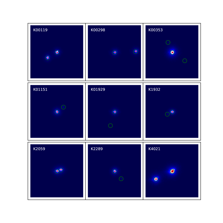
Figure 1.— AO images for 9 KOIs with newly detected stellar companions within 2^′′. All images cover a 2^′′ by 2^′′ sky region centering at the primary star. North is up and east is to the left. Linear color scale is chosen such that the central star (red) is normalized to 1 and the background (blue) represents 1/100 of the central star flux. Both central stars and detected stellar companions are marked by green circles. Photometric and astrometric information of detected stellar companions can be found in Table 2.

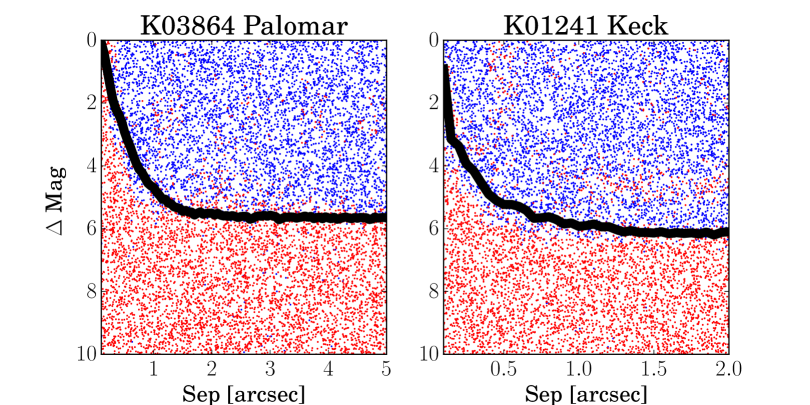
Figure 2.— Simulation for AO search completeness in comparison with contrast curve. Left panel shows an example for a Palomar AO image and right panel for a Keck AO image. Blue dots are artificial PSF injections at random separations, differential magnitudes and position angles that are successfully recovered by our detection pipeline. Red dots are injections that are missed. AO contrast curves (§3.1) are plotted as black solid lines which generally trace the border line between blue and red dots.

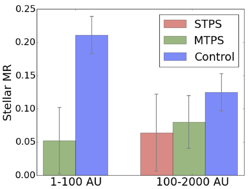
Figure 3.— Stellar multiplicity rate for multiple transiting planet systems (MTPS, green), single transiting planet systems (STPS, red), and the field stars in the solar neighborhood, i.e., the control sample in blue. The stellar multiplicity rates for different samples are given in Table 5.

Table 1AO Sensitivity

Kepler							Observation				Limiting Delta Magnitude∗∗
KIC	KOI	Kmag	$i$	$J$	$H$	$K$	Comp.	Iso.	Instrument	Flt	0.1	0.2	0.5	1.0	2.0	4.0
		[mag]	[mag]	[mag]	[mag]	[mag]	$<$ 5′′	Prob.∗			[′′]	[′′]	[′′]	[′′]	[′′]	[′′]
8554498	00005	11.665	11.485	10.542	10.257	10.213	yes	$\cdots$	NIRC2	K	2.0	4.0	6.4	7.4	7.5	7.5
8554498	00005	11.665	11.485	10.542	10.257	10.213	yes	$\cdots$	PHARO	J	0.1	1.3	2.7	4.8	6.7	7.6
6521045	00041	11.197	11.030	10.081	9.804	9.768	no	0.96	ARIES	K	0.1	1.2	3.4	5.9	7.2	7.5
6521045	00041	11.197	11.030	10.081	9.804	9.768	no	0.96	NIRC2	K	3.2	4.6	5.3	5.4	5.4	5.4
6521045	00041	11.197	11.030	10.081	9.804	9.768	no	0.96	PHARO	J	0.4	3.6	4.5	6.6	7.6	7.7
6850504	00070	12.498	12.284	11.252	10.910	10.871	yes	$\cdots$	PHARO	J	0.4	3.0	4.5	6.4	7.3	7.4
11904151	00072	10.961	10.778	9.889	9.563	9.496	no	0.99	ARIES	K	0.8	2.3	5.1	7.0	7.6	7.6
11904151	00072	10.961	10.778	9.889	9.563	9.496	no	0.99	PHARO	J	0.5	3.3	4.3	6.5	7.9	8.1
10187017	00082	11.492	11.150	9.984	9.446	9.351	no	0.92	ARIES	K	0.5	1.9	4.7	7.0	7.8	7.9
10187017	00082	11.492	11.150	9.984	9.446	9.351	no	0.92	NIRC2	K	2.6	4.5	5.4	5.6	5.6	5.6
5866724	00085	11.018	10.882	10.066	9.852	9.806	no	0.88	ARIES	K	0.9	2.4	5.1	7.1	7.6	7.7
6462863	00094	12.205	12.057	11.218	10.957	10.926	no	0.75	ARIES	K	0.1	0.9	4.2	6.8	7.4	7.3
8456679	00102	12.566	12.384	11.398	11.124	11.055	yes	$\cdots$	NIRC2	K	2.2	4.3	6.3	7.2	7.3	7.3
8456679	00102	12.566	12.384	11.398	11.124	11.055	yes	$\cdots$	PHARO	J	0.7	2.2	4.0	5.8	6.9	7.4
4914423	00108	12.287	12.132	11.193	10.941	10.873	yes	$\cdots$	NIRC2	K	2.5	4.0	5.7	6.1	6.2	6.2
4914423	00108	12.287	12.132	11.193	10.941	10.873	yes	$\cdots$	PHARO	J	0.8	3.2	4.4	6.5	7.6	7.7
6678383	00111	12.596	12.442	11.558	11.251	11.209	no	0.89	PHARO	J	0.6	2.9	4.2	6.1	7.1	7.3
10984090	00112	12.772	12.602	11.698	11.402	11.367	no	0.84	PHARO	J	0.5	2.4	3.9	6.1	8.0	8.5
10984090	00112	12.772	12.602	11.698	11.402	11.367	no	0.84	PHARO	K	0.0	1.8	4.8	5.4	6.9	7.1
9579641	00115	12.791	12.654	11.811	11.555	11.503	yes	$\cdots$	ARIES	K	0.2	1.8	4.9	6.6	6.8	6.8
8395660	00116	12.882	12.706	11.752	11.494	11.431	no	0.91	ARIES	K	0.4	1.9	4.9	7.0	7.3	7.2
8395660	00116	12.882	12.706	11.752	11.494	11.431	no	0.91	NIRC2	K	2.9	4.5	6.2	6.5	6.6	6.6
10875245	00117	12.487	12.309	11.392	11.114	11.060	no	0.74	PHARO	J	0.1	0.7	2.1	3.7	5.9	7.9
10875245	00117	12.487	12.309	11.392	11.114	11.060	no	0.74	PHARO	K	0.4	1.5	3.6	5.0	6.8	7.2
9471974	00119	12.654	12.452	11.430	11.065	10.983	yes	$\cdots$	PHARO	J	0.0	0.6	1.8	3.3	4.5	7.3
9471974	00119	12.654	12.452	11.430	11.065	10.983	yes	$\cdots$	PHARO	K	0.0	0.7	2.7	4.3	5.5	6.5
5094751	00123	12.365	12.206	11.314	11.046	11.001	no	0.86	NIRC2	K	2.4	4.3	6.0	6.5	6.5	6.5
5094751	00123	12.365	12.206	11.314	11.046	11.001	no	0.86	PHARO	J	0.0	1.2	3.3	5.3	7.0	7.6
5735762	00148	13.040	12.761	11.702	11.292	11.221	yes	$\cdots$	NIRC2	K	2.3	4.2	5.7	6.3	6.3	6.3
5735762	00148	13.040	12.761	11.702	11.292	11.221	yes	$\cdots$	PHARO	J	0.2	2.8	4.0	6.1	7.4	7.6
12252424	00153	13.461	13.097	11.886	11.360	11.255	no	0.93	ARIES	K	0.0	1.0	4.1	6.4	6.7	6.7
12252424	00153	13.461	13.097	11.886	11.360	11.255	no	0.93	NIRC2	K	2.0	4.2	4.9	4.9	4.9	4.9
12252424	00153	13.461	13.097	11.886	11.360	11.255	no	0.93	PHARO	J	0.1	0.9	2.2	3.9	6.1	7.6
12252424	00153	13.461	13.097	11.886	11.360	11.255	no	0.93	PHARO	K	0.5	1.7	3.7	5.0	6.6	6.8
11512246	00168	13.438	13.244	12.353	12.047	11.998	no	0.69	PHARO	K	0.4	1.4	3.3	4.8	5.5	5.6
4349452	00244	10.734		9.764	9.532	9.493	no	0.91	NIRC2	K	2.8	4.4	5.3	5.4	5.4	5.4
4349452	00244	10.734		9.764	9.532	9.493	no	0.91	PHARO	J	0.6	2.7	3.9	5.8	7.9	8.5
4349452	00244	10.734		9.764	9.532	9.493	no	0.91	PHARO	K	0.8	2.7	5.0	5.6	7.7	8.1
8478994	00245	9.705		8.356	8.000	7.942	no	0.95	ARIES	K	0.5	1.8	4.8	7.3	8.2	8.4
8478994	00245	9.705		8.356	8.000	7.942	no	0.95	NIRC2	K	2.4	4.1	6.1	6.7	6.9	6.9
8478994	00245	9.705		8.356	8.000	7.942	no	0.95	PHARO	K	1.0	2.3	5.0	6.7	8.6	9.9
11295426	00246	9.997	9.820	8.975	8.662	8.588	no	0.97	ARIES	K	0.6	2.0	4.4	6.8	7.7	7.8
11295426	00246	9.997	9.820	8.975	8.662	8.588	no	0.97	NIRC2	K	2.9	4.4	6.0	6.3	6.4	6.4
8292840	00260	10.500		9.616	9.407	9.344	no	0.92	ARIES	K	0.1	1.5	3.7	6.2	7.7	8.2
11807274	00262	10.421	10.313	9.518	9.250	9.197	no	0.89	ARIES	K	0.7	2.5	4.8	6.8	7.3	7.5
6528464	00270	11.411		10.088	9.770	9.701	no	0.80	ARIES	K	0.2	1.7	4.0	6.1	7.0	7.1
9451706	00271	11.485	11.358	10.536	10.300	10.234	no	0.90	ARIES	K	0.7	2.3	4.6	6.8	7.2	7.4
9451706	00271	11.485	11.358	10.536	10.300	10.234	no	0.90	NIRC2	K	2.7	4.5	6.6	7.4	7.5	7.5
9451706	00271	11.485	11.358	10.536	10.300	10.234	no	0.90	PHARO	J	0.7	2.4	4.5	5.5	7.5	7.8
9451706	00271	11.485	11.358	10.536	10.300	10.234	no	0.90	PHARO	K	0.0	0.9	2.4	4.1	5.4	5.8
8077137	00274	11.390	11.258	10.373	10.094	10.109	no	0.88	ARIES	K	0.7	2.4	5.2	7.1	7.6	7.7
10586004	00275	11.696		10.600	10.325	10.252	no	0.86	PHARO	J	1.2	2.7	5.2	5.9	7.5	7.7
10586004	00275	11.696		10.600	10.325	10.252	no	0.86	PHARO	K	0.5	2.5	3.7	5.9	8.0	8.7
12314973	00279	11.684	11.563	10.708	10.472	10.429	yes	$\cdots$	NIRC2	K	2.1	4.3	5.5	5.6	5.7	5.7
5088536	00282	11.529		10.810	10.529	10.490	yes	$\cdots$	NIRC2	K	2.4	4.3	6.6	7.4	7.5	7.5
5088536	00282	11.529		10.810	10.529	10.490	yes	$\cdots$	PHARO	K	0.5	1.5	3.6	5.7	7.3	7.6
5695396	00283	11.525	11.334	10.418	10.127	10.079	no	0.95	NIRC2	K	2.5	3.9	5.2	5.5	5.5	5.5
5695396	00283	11.525	11.334	10.418	10.127	10.079	no	0.95	PHARO	J	0.0	0.5	1.7	3.1	5.2	7.4
5695396	00283	11.525	11.334	10.418	10.127	10.079	no	0.95	PHARO	K	0.8	2.2	4.1	5.8	7.3	7.7
6021275	00284	11.818	11.666	10.797	10.516	10.424	yes	$\cdots$	PHARO	J	0.0	0.2	1.7	3.2	4.6	5.8
6021275	00284	11.818	11.666	10.797	10.516	10.424	yes	$\cdots$	PHARO	K	0.0	0.4	1.6	3.7	5.1	7.9
6196457	00285	11.565		10.747	10.470	10.403	yes	$\cdots$	PHARO	J	0.0	0.7	2.1	3.9	5.9	7.0
6196457	00285	11.565		10.747	10.470	10.403	yes	$\cdots$	PHARO	K	0.4	1.9	3.9	5.6	7.1	7.5
10386922	00289	12.747	12.540	11.534	11.220	11.187	no	0.92	NIRC2	K	2.5	4.5	6.5	7.2	7.3	7.3
10386922	00289	12.747	12.540	11.534	11.220	11.187	no	0.92	PHARO	K	0.2	1.0	3.1	5.0	6.2	6.5
10933561	00291	12.848	12.642	11.680	11.399	11.320	no	0.69	PHARO	K	0.3	1.0	3.0	4.5	5.0	5.1
11547513	00295	12.324	12.155	11.260	10.984	10.951	no	0.77	PHARO	K	0.9	1.8	3.6	5.7	6.7	6.9
12785320	00298	12.713	12.355	11.295	10.946	10.885	yes	$\cdots$	PHARO	J	0.0	0.5	1.9	3.3	5.0	5.8
12785320	00298	12.713	12.355	11.295	10.946	10.885	yes	$\cdots$	PHARO	K	0.5	1.2	3.1	4.5	4.9	5.8
3642289	00301	12.730	12.586	11.722	11.508	11.456	no	0.72	PHARO	K	0.0	0.9	3.0	4.7	5.3	5.4
6029239	00304	12.549	12.377	11.472	11.192	11.109	no	0.83	PHARO	K	0.7	1.7	4.2	5.6	6.5	6.7
6289257	00307	12.797	12.650	11.806	11.552	11.488	no	0.73	PHARO	K	0.0	0.9	3.1	4.7	5.2	5.3
7050989	00312	12.459		10.804	10.573	10.519	yes	$\cdots$	NIRC2	K	1.4	3.3	5.4	6.0	6.1	6.0
7050989	00312	12.459		10.804	10.573	10.519	yes	$\cdots$	PHARO	K	0.2	1.3	3.2	5.5	7.1	7.7
7419318	00313	12.990	12.736	11.650	11.229	11.165	no	0.81	PHARO	J	0.4	1.3	2.8	4.8	7.1	8.1
7419318	00313	12.990	12.736	11.650	11.229	11.165	no	0.81	PHARO	K	0.5	1.8	3.7	5.3	6.9	7.1
7603200	00314	12.925	12.457	10.293	9.680	9.506	no	0.91	PHARO	K	0.3	1.1	3.0	4.9	6.3	6.6
8008067	00316	12.701	12.494	11.530	11.222	11.167	no	0.82	PHARO	J	0.0	0.5	1.6	3.2	5.4	6.9
8008067	00316	12.701	12.494	11.530	11.222	11.167	no	0.82	PHARO	K	0.3	1.4	3.2	4.9	6.1	6.4
8753657	00321	12.520	12.312	11.340	11.035	10.970	no	0.92	NIRC2	K	2.8	4.3	6.1	6.7	6.8	6.8
9880467	00326	12.960	12.960	14.774	13.236	13.085	yes	$\cdots$	PHARO	K	0.1	1.0	3.9	4.6	4.9	4.9
9881662	00327	12.996	12.858	11.989	11.759	11.709	no	0.91	PHARO	K	0.1	0.9	2.7	4.2	4.6	4.7
10290666	00332	13.046	12.847	11.910	11.569	11.475	no	0.76	PHARO	K	0.2	0.8	2.5	4.2	5.4	5.6
10552611	00338	13.448	13.116	11.955	11.485	11.393	no	0.68	PHARO	K	0.5	1.5	3.6	5.3	6.3	6.3
10878263	00341	13.338	13.106	12.087	11.750	11.698	no	0.71	ARIES	K	0.0	0.5	2.4	4.9	6.0	6.1
10982872	00343	13.203	13.013	12.092	11.801	11.762	no	0.73	PHARO	K	0.3	1.1	2.7	4.5	5.4	5.5
11566064	00353	13.374	13.251	12.455	12.263	12.228	yes	$\cdots$	PHARO	K	0.1	0.9	2.4	3.6	4.6	4.8
11568987	00354	13.235	13.057	12.063	11.775	11.708	yes	$\cdots$	PHARO	K	0.2	0.9	2.6	4.4	5.4	5.5
7175184	00369	11.992	11.868	11.050	10.830	10.792	no	0.76	PHARO	K	0.2	1.0	3.0	4.9	5.8	6.1
12068975	00623	11.811	11.685	10.814	10.577	10.535	no	0.85	NIRC2	K	2.0	4.1	6.0	6.4	6.5	6.5
4478168	00626	13.490	13.339	12.514	12.195	12.205	yes	$\cdots$	PHARO	K	0.8	1.8	4.5	5.5	5.8	6.0
4563268	00627	13.307	13.119	12.203	11.938	11.905	no	0.69	PHARO	K	0.0	0.3	2.1	4.1	5.9	7.0
5966154	00655	13.004	12.872	12.037	11.784	11.737	no	0.75	PHARO	K	0.0	1.0	2.4	4.3	5.1	5.2
6685609	00665	13.182	13.005	12.100	11.841	11.805	no	0.71	PHARO	K	0.3	1.3	2.9	4.5	5.4	5.5
7509886	00678	13.283	12.997	11.927	11.488	11.447	no	0.75	PHARO	K	0.1	1.0	2.8	4.5	5.5	5.7
7515212	00679	13.178	13.038	11.931	11.699	11.620	no	0.74	PHARO	K	0.4	1.3	3.0	4.7	5.7	5.9
9590976	00710	13.294	13.128	12.319	12.176	12.103	no	0.68	PHARO	K	0.0	1.0	2.6	4.2	5.0	5.1
9873254	00717	13.387	13.182	12.194	11.868	11.793	no	0.72	PHARO	K	0.2	1.3	3.2	4.7	5.6	5.8
9950612	00719	13.177	12.899	11.206	10.672	10.550	no	0.94	NIRC2	K	2.7	4.5	6.6	7.8	8.0	8.0
11013201	00972	9.275	9.392	8.816	8.765	8.736	no	0.86	PHARO	K	1.3	2.5	5.1	6.8	8.8	9.3
1871056	01001	13.038	12.851	11.918	11.692	11.591	yes	$\cdots$	PHARO	K	0.2	1.0	2.7	4.4	5.4	5.6
8280511	01151	13.404	13.198	12.198	11.819	11.745	yes	$\cdots$	PHARO	K	0.3	1.3	3.1	4.6	5.7	5.8
10350571	01175	13.290	13.075	12.061	11.704	11.617	no	0.67	PHARO	K	0.0	0.8	2.4	4.1	5.2	5.4
3939150	01215	13.420	13.226	12.288	12.003	11.966	no	0.68	PHARO	K	0.5	1.4	3.5	5.1	5.7	5.8
6448890	01241	12.440	12.090	10.813	10.330	10.227	no	0.81	NIRC2	K	2.1	3.6	5.4	6.0	6.1	6.0
6448890	01241	12.440	12.090	10.813	10.330	10.227	no	0.81	PHARO	K	0.1	0.9	2.8	5.0	6.8	7.5
10794087	01316	11.926	11.694	10.894	10.606	10.562	yes	$\cdots$	ARIES	K	0.4	1.6	3.5	5.8	7.9	8.2
10794087	01316	11.926	11.694	10.894	10.606	10.562	yes	$\cdots$	NIRC2	K	2.4	4.4	6.9	7.6	7.7	7.7
11336883	01445	12.320	12.209	11.406	11.171	11.151	no	0.86	PHARO	K	0.2	1.0	2.8	4.9	6.4	6.9
7869917	01525	12.082	12.009	11.250	11.065	11.039	no	0.71	PHARO	K	0.4	1.1	3.0	4.9	6.5	7.1
4741126	01534	13.470	13.325	12.539	12.270	12.241	no	0.69	PHARO	K	0.4	1.1	3.0	4.5	5.1	5.2
6268648	01613	11.049		10.588	10.316	10.282	yes	$\cdots$	NIRC2	K	2.4	4.5	6.3	7.6	7.7	7.7
6268648	01613	11.049		10.588	10.316	10.282	yes	$\cdots$	PHARO	K	0.0	0.4	4.4	5.9	7.0	7.3
6975129	01628	12.949	12.775	11.902	11.664	11.596	no	0.83	PHARO	K	0.2	1.0	2.9	4.5	4.9	5.0
6616218	01692	12.557	12.313	11.242	10.850	10.778	yes	$\cdots$	PHARO	K	0.2	1.0	4.1	5.3	6.4	6.8
9909735	01779	13.297	13.077	12.148	11.832	11.766	no	0.80	NIRC2	K	1.8	4.1	5.2	5.5	5.5	5.4
9909735	01779	13.297	13.077	12.148	11.832	11.766	no	0.80	PHARO	K	0.1	1.0	2.7	4.5	5.5	5.6
11551692	01781	12.231	11.884	10.641	10.161	10.062	yes	$\cdots$	NIRC2	J	1.7	2.6	4.2	5.5	5.8	5.6
11551692	01781	12.231	11.884	10.641	10.161	10.062	yes	$\cdots$	NIRC2	K	1.5	3.3	5.1	5.8	5.9	5.8
11551692	01781	12.231	11.884	10.641	10.161	10.062	yes	$\cdots$	PHARO	K	0.1	1.1	3.0	5.2	6.8	7.3
9529744	01806	13.474	13.337	12.546	12.283	12.307	yes	$\cdots$	PHARO	K	0.3	1.2	3.1	4.5	5.0	4.9
8240797	01809	12.706	12.474	11.621	11.300	11.249	no	0.73	PHARO	K	0.2	1.0	3.1	5.3	6.1	6.2
2989404	01824	12.722	12.567	11.689	11.423	11.354	no	0.73	PHARO	K	0.3	1.3	3.3	5.0	5.9	6.0
10130039	01909	12.776	12.612	11.710	11.448	11.409	no	0.73	PHARO	K	0.3	1.2	3.2	4.8	5.6	5.7
10136549	01929	12.727	12.530	11.537	11.257	11.183	yes	$\cdots$	PHARO	K	0.3	1.1	3.2	4.9	5.7	5.8
5511081	01930	12.119	11.957	11.098	10.841	10.756	no	0.85	NIRC2	K	2.6	4.6	6.7	7.3	7.4	7.4
5202905	01932	12.345	12.366	11.725	11.629	11.583	yes	$\cdots$	NIRC2	H	1.4	2.8	4.4	5.1	5.3	5.3
5202905	01932	12.345	12.366	11.725	11.629	11.583	yes	$\cdots$	NIRC2	J	1.3	2.4	3.9	5.0	5.3	5.2
5202905	01932	12.345	12.366	11.725	11.629	11.583	yes	$\cdots$	NIRC2	K	1.5	3.8	4.9	5.4	5.4	5.3
5202905	01932	12.345	12.366	11.725	11.629	11.583	yes	$\cdots$	PHARO	K	0.2	1.1	3.1	5.3	6.6	6.8
9892816	01955	13.147	13.025	12.220	11.999	11.957	no	0.76	PHARO	K	0.3	1.1	3.0	4.6	5.3	5.4
12154526	02004	13.351	13.150	12.174	11.872	11.803	no	0.78	PHARO	K	0.4	1.2	2.8	4.5	5.5	5.7
5384079	02011	12.556	12.419	11.708	11.454	11.377	yes	$\cdots$	PHARO	K	0.1	0.9	2.7	4.8	6.2	6.5
9489524	02029	12.957	12.694	11.610	11.178	11.132	no	0.91	NIRC2	K	2.2	4.4	6.4	7.3	7.3	7.3
2307415	02053	12.992	12.839	12.000	11.745	11.704	no	0.71	PHARO	K	0.1	0.8	2.5	4.2	4.7	4.7
12301181	02059	12.906	12.558	11.305	10.791	10.664	yes	$\cdots$	NIRC2	K	2.4	4.0	5.6	7.4	7.8	7.8
12301181	02059	12.906	12.558	11.305	10.791	10.664	yes	$\cdots$	PHARO	K	0.0	0.0	1.7	3.6	4.8	4.9
6021193	02148	13.353	13.112	12.111	11.755	11.697	no	0.68	PHARO	K	0.5	1.5	3.6	5.2	6.0	6.2
9006186	02169	12.404	12.172	11.137	10.735	10.662	yes	$\cdots$	PHARO	K	0.2	1.1	2.9	5.0	6.8	7.1
11774991	02173	12.879	12.522	11.243	10.752	10.674	no	0.94	NIRC2	K	2.8	4.6	6.6	7.3	7.5	7.4
9022166	02175	12.848	12.626	11.600	11.229	11.175	no	0.85	NIRC2	K	2.9	4.6	6.5	7.1	7.2	7.2
3867615	02289	13.358	13.193	12.341	12.092	12.005	yes	$\cdots$	PHARO	K	0.3	1.3	3.1	4.6	5.6	5.7
8013439	02352	10.421		9.721	9.547	9.504	no	0.92	NIRC2	K	2.5	4.6	6.8	7.5	7.5	7.5
8013439	02352	10.421		9.721	9.547	9.504	no	0.92	PHARO	K	1.1	2.7	5.0	6.8	7.8	8.1
12306058	02541	13.007	12.717	11.564	11.072	10.970	no	0.66	PHARO	K	0.2	0.9	2.7	4.6	5.8	6.1
8883329	02595	13.223	13.107	12.325	12.087	11.995	no	0.68	PHARO	K	0.2	1.0	2.6	4.4	5.5	5.7
11253827	02672	11.921	11.703	10.672	10.356	10.285	yes	$\cdots$	PHARO	K	0.2	1.4	4.0	5.9	6.8	6.8
8022489	02674	13.349	13.159	12.169	11.859	11.825	no	0.81	PHARO	K	0.5	1.5	3.1	4.8	5.6	5.7
7202957	02687	10.158	9.973	9.052	8.761	8.693	no	0.88	PHARO	K	0.9	2.9	5.6	7.5	8.8	8.9
11071200	02696	12.998	12.901	12.188	12.032	11.950	no	0.66	PHARO	K	0.0	0.7	2.2	4.0	4.7	4.8
12206313	02714	13.312	13.160	12.277	12.065	11.987	no	0.71	PHARO	K	0.3	1.3	3.1	4.7	5.4	5.5
6026737	02949	13.313	13.135	12.222	11.973	11.903	yes	$\cdots$	PHARO	K	0.5	1.6	3.4	5.2	5.8	5.9
6278762	03158	8.717		7.244	6.772	6.703	yes	$\cdots$	NIRC2	K	2.7	4.6	5.8	6.1	6.1	6.1
6278762	03158	8.717		7.244	6.772	6.703	yes	$\cdots$	PHARO	J	0.0	1.6	3.5	5.3	7.1	8.9
6278762	03158	8.717		7.244	6.772	6.703	yes	$\cdots$	PHARO	K	1.5	3.4	5.8	7.4	8.9	9.7
9002538	03196	11.525	11.405	10.547	10.335	10.276	no	0.90	NIRC2	K	2.6	4.4	6.6	7.5	7.6	7.6
9002538	03196	11.525	11.405	10.547	10.335	10.276	no	0.90	PHARO	K	0.3	1.3	3.9	5.5	6.6	7.0
8644365	03384	13.204	13.008	12.022	11.757	11.724	no	0.72	PHARO	K	0.4	1.4	3.1	4.8	5.7	5.8
3561464	03398	13.489	13.361	12.556	12.311	12.289	no	0.80	PHARO	K	0.9	2.4	4.9	5.5	5.9	5.9
11754430	03403	13.102	12.921	12.012	11.694	11.638	no	0.79	PHARO	K	0.2	1.1	2.9	4.7	5.6	5.7
9117416	03425	13.266	12.957	11.897	11.610	11.514	no	0.84	NIRC2	K	2.3	4.3	6.4	7.2	7.3	7.3
6058816	03500	13.214	13.038	12.161	11.870	11.826	yes	$\cdots$	PHARO	K	0.3	1.1	2.9	4.4	5.2	5.4
2581316	03681	11.690		10.953	10.728	10.688	no	0.92	NIRC2	K	2.2	4.6	5.8	5.9	5.9	5.9
4164922	03864	12.914	12.604	11.489	11.013	10.915	no	0.77	PHARO	K	0.1	1.0	2.9	4.7	5.5	5.6
11967788	04021	13.166	12.513	11.797	11.538	11.487	yes	$\cdots$	PHARO	K	0.0	0.4	1.8	2.9	4.0	4.4
7100673	04032	12.639	12.432	11.421	11.034	10.989	no	0.77	PHARO	K	0.0	0.6	1.9	4.1	6.0	6.4
5688683	04097	13.435	12.965	11.614	10.958	10.841	no	0.85	PHARO	K	0.3	1.4	3.3	5.1	6.2	6.5
8890924	04269	13.263	12.943	11.718	11.249	11.136	no	0.79	PHARO	K	0.0	0.9	2.5	4.4	5.7	6.0
4548011	04288	12.400	12.246	11.331	11.106	11.025	yes	$\cdots$	PHARO	K	0.3	1.1	3.0	5.3	6.7	7.1

Note. — ^∗: Isolation probability is the probability of a KOI being isolated within 2000 AU (i.e., has no stellar companion within 2000 AU) given the AO and/or RV data and/or dynamical analysis (see §3.3). For stars with detected nearby stellar companions, the physical association probability can be found in Table 2. ^∗∗: Limiting Delta Magnitudes are 5-$\sigma$ limit.

Table 2Visual companion detections with AO data for Kepler MTPS.

KOI	Star#	Telescope	Filter	$\Delta$ Mag∗	Separation∗∗		Distance∗∗∗		PA	Association∗∗∗∗	ref.†
							Primary	Secondary		Probability
				(mag)	(arcsec)	(AU)	(pc)	(pc)	(deg)
K00005	1	Keck	K	2.20	0.14	40.12	$286.6^{71.1}_{-15.8}$		307.4	$>0.90$	CFOP
K00070	1	Palomar	J	4.41	3.77	1052.60	$279.5^{25.3}_{-23.6}$		51.8	0.52	A12
K00102	1	Palomar	J	1.12	2.84	934.31	$329.4^{75.0}_{-30.5}$		222.2	$>0.90$	A12
K00108	1	Palomar	J	5.71	2.51	891.07	$354.6^{45.4}_{-39.2}$		285.2	0.48	A12
K00108	2	Palomar	J	5.60	3.23	1145.12	$354.6^{45.4}_{-39.2}$		100.8	0.30	A12
K00108	3	Palomar	J	6.60	5.00	1773.09	$354.6^{45.4}_{-39.2}$		112.5	0.00	A12
K00115	1	MMT	K	5.06	4.00	2168.27	$542.1^{140.6}_{-97.0}$		89.7	0.33	A12
K00119	1	Palomar	J	0.16	1.05	327.89	$313.0^{106.8}_{-62.2}$	$380.8^{499.6}_{-154.5}$	119.1	$>0.90$	this work
K00119	1	Palomar	K	0.22	1.04	326.17	$313.0^{106.8}_{-62.2}$	$380.8^{499.6}_{-154.5}$	120.2	$>0.90$	this work
K00148	1	Palomar	J	4.75	2.51	775.44	$308.7^{27.0}_{-17.2}$		245.6	0.78	A12
K00148	2	Palomar	J	3.14	4.43	1368.74	$308.7^{27.0}_{-17.2}$		220.4	0.73	A12
K00279	1	Keck	K	2.35	0.92	247.44	$268.6^{187.6}_{-46.3}$		247.3	$>0.90$	CFOP
K00282	1	Palomar	K	3.86	4.16	1408.24	$338.8^{16.9}_{-26.5}$		210.3	0.84	CFOP
K00284	1	Palomar	J	0.24	0.87	229.45	$264.7^{34.4}_{-39.4}$	$339.5^{347.4}_{-146.8}$	95.8	$>0.90$	A12
K00284	1	Palomar	K	0.24	0.86	226.48	$264.7^{34.4}_{-39.4}$	$339.5^{347.4}_{-146.8}$	96.7	$>0.90$	A12
K00285	1	Palomar	J	4.19	1.50	676.86	$452.7^{18.4}_{-47.0}$	$3855.9^{2632.5}_{-3163.9}$	137.7	$>0.90$	CFOP
K00285	1	Palomar	K	4.08	1.50	677.09	$452.7^{18.4}_{-47.0}$	$3855.9^{2632.5}_{-3163.9}$	137.7	$>0.90$	CFOP
K00298	1	Palomar	J	0.24	2.00	581.07	$290.2^{300.0}_{-54.4}$	$247.2^{335.0}_{-68.1}$	272.8	$>0.90$	this work
K00298	1	Palomar	K	0.08	1.96	570.05	$290.2^{300.0}_{-54.4}$	$247.2^{335.0}_{-68.1}$	272.5	$>0.90$	this work
K00312	1	Palomar	K	6.67	3.01	950.62	$316.1^{33.3}_{-25.9}$		104.4	0.34	this work
K00312	2	Palomar	K	5.84	4.97	1569.91	$316.1^{33.3}_{-25.9}$		121.7	0.33	this work
K00326	1	Palomar	K	1.03	3.49	27865.11	$7989.4^{1953.2}_{-1200.3}$		269.4	0.89	this work
K00353	1	Palomar	K	3.07	1.04	820.45	$789.7^{151.9}_{-103.2}$		23.0	$>0.90$	this work
K00353	2	Palomar	K	4.15	1.43	1131.97	$789.7^{151.9}_{-103.2}$		236.3	$>0.90$	this work
K00354	1	Palomar	K	4.83	3.73	1425.50	$382.1^{29.8}_{-25.5}$		210.1	0.36	this work
K00626	1	Palomar	K	5.30	2.75	1463.00	$532.3^{39.1}_{-43.4}$		167.9	0.21	this work
K01151	1	Palomar	K	2.25	0.76	316.71	$419.5^{53.7}_{-50.0}$		306.6	$>0.90$	this work
K01316	1	MMT	K	5.81	2.78	1249.69	$449.6^{185.2}_{-96.3}$		4.8	0.68	CFOP (Dupree)
K01613	1	Keck	K	1.00	0.22	79.49	$364.3^{21.7}_{-19.1}$		184.6	$>0.90$	CFOP
K01613	1	Palomar	K	1.16	0.21	75.31	$364.3^{21.7}_{-19.1}$		183.4	$>0.90$	CFOP
K01692	1	Palomar	K	6.36	3.17	841.66	$265.4^{14.6}_{-19.8}$		337.2	0.31	this work
K01781	1	Keck	J	2.71	3.48	607.66	$174.8^{10.7}_{-14.8}$	$508.7^{569.0}_{-178.8}$	332.4	$>0.90$	this work
K01781	1	Keck	K	2.35	3.47	606.92	$174.8^{10.7}_{-14.8}$	$508.7^{569.0}_{-178.8}$	332.2	$>0.90$	this work
K01781	1	Palomar	K	2.29	3.43	599.24	$174.8^{10.7}_{-14.8}$	$508.7^{569.0}_{-178.8}$	332.4	$>0.90$	this work
K01806	1	Palomar	K	1.45	3.43	2096.38	$612.1^{62.3}_{-70.2}$		249.7	0.90	this work
K01929	1	Palomar	K	4.86	1.37	835.32	$608.8^{64.2}_{-162.1}$		163.0	$>0.90$	this work
K01932	1	Keck	J	4.08	0.54	1165.27	$2171.2^{444.3}_{-885.7}$	$10489.3^{2415.5}_{-10378.5}$	116.6	$>0.90$	this work
K01932	1	Keck	H	3.37	0.52	1129.01	$2171.2^{444.3}_{-885.7}$	$10489.3^{2415.5}_{-10378.5}$	115.3	$>0.90$	this work
K01932	1	Keck	K	3.12	0.52	1138.78	$2171.2^{444.3}_{-885.7}$	$10489.3^{2415.5}_{-10378.5}$	115.1	$>0.90$	this work
K01932	2	Palomar	K	4.12	4.57	9928.21	$2171.2^{444.3}_{-885.7}$		312.9	0.51	this work
K02011	1	Palomar	K	2.73	4.95	2312.74	$467.1^{59.2}_{-68.5}$		292.1	0.82	this work
K02059	1	Keck	K	0.14	0.39	92.93	$238.4^{13.8}_{-15.7}$		289.5	$>0.90$	this work
K02059	1	Palomar	K	0.14	0.38	91.43	$238.4^{13.8}_{-15.7}$		289.0	$>0.90$	this work
K02169	1	Palomar	K	2.74	3.49	1026.94	$294.1^{97.4}_{-29.0}$		289.0	$>0.90$	this work
K02289	1	Palomar	K	2.78	0.94	535.74	$570.5^{99.2}_{-67.8}$		221.2	$>0.90$	this work
K02672	1	Palomar	K	3.46	0.65	152.28	$236.0^{126.7}_{-46.5}$		305.5	$>0.90$	CFOP
K02672	2	Palomar	K	6.04	4.62	1090.18	$236.0^{126.7}_{-46.5}$		310.5	0.26	this work
K02949	1	Palomar	K	3.86	2.35	1442.31	$613.1^{598.6}_{-111.5}$		311.0	0.81	this work
K03158	1	Palomar	J	2.39	1.83	54.30	$29.6^{1.4}_{-3.1}$	$78.8^{53.8}_{-64.7}$	253.3	$>0.90$	C15
K03158	1	Keck	K	2.21	1.86	55.05	$29.6^{1.4}_{-3.1}$	$78.8^{53.8}_{-64.7}$	252.8	$>0.90$	C15
K03158	1	Palomar	K	2.13	1.83	54.35	$29.6^{1.4}_{-3.1}$	$78.8^{53.8}_{-64.7}$	253.1	$>0.90$	C15
K03500	1	Palomar	K	3.35	2.53	1150.97	$455.2^{60.4}_{-44.7}$		140.0	0.90	this work
K04021	1	Palomar	K	0.33	1.74	1886.56	$1085.2^{303.3}_{-221.0}$		115.8	$>0.90$	this work
K04288	1	Palomar	K	6.59	2.93	1039.80	$354.8^{61.1}_{-37.1}$		279.8	0.03	this work

Note. — References: A12 - Adams et al. (2012); C15 - Campante et al. (2015). ^∗: Typical $\Delta$ Mag uncertainty is 0.1 mag. The uncertainty is estimated from the companion injection simulation described in §3.3. ^∗∗: Typical angular separation uncertainty is 0.05^′′. The uncertainty is estimated from the companion injection simulation described in §3.3. ^∗∗∗: Distance is estimated based on stellar properties of primary stars (Huber et al., 2014) and color information of secondary stars (see §4.1 in Wang et al., 2015, for more details). ^∗∗∗∗: Association probability has 10% uncertainty due to statistical error in simulation. ^†: AO images from CFOP are provided by David Ciardi unless otherwise noted.

Table 3Stellar Parameters For STPS

KOI	KIC	$\alpha$	$\delta$	$Kp$	$T_{\rm eff}$	$\log g$	[Fe/H]
		(h:m:s)	(d:m:s)	(mag)	(K)	(cgs)	(dex)
00042	8866102	18:52:36.17	45:08:23.4	9.36	6325	4.26	0.01
00069	3544595	19:25:40.39	38:40:20.49	9.93	5669	4.47	-0.18
00084	2571238	19:21:40.99	37:51:06.48	11.90	5543	4.57	-0.14
00087	10593626	19:16:52.2	47:53:04.06	11.66	5642	4.44	-0.27
00092	7941200	18:53:29.96	43:47:17.59	11.67	5952	4.49	-0.04
00103	2444412	19:26:44	37:45:05.73	12.59	5653	4.55	-0.06
00118	3531558	19:09:27.07	38:38:58.56	12.38	5747	4.18	0.03
00122	8349582	18:57:55.79	44:23:52.95	12.35	5699	4.17	0.30
00180	9573539	18:57:34.63	46:14:56.69	13.02	5691	4.54	-0.06
00257	5514383	18:58:32.45	40:43:11.39	10.87	6184	4.36	0.12
00261	5383248	19:48:16.71	40:31:30.47	10.30	5763	4.53	0.04
00265	12024120	19:48:04.52	50:24:32.33	11.99	6036	4.32	0.08
00268	3425851	19:02:54.91	38:30:25.1	10.56	6343	4.26	-0.04
00269	7670943	19:09:22.98	43:22:42.21	10.93	6463	4.24	0.09
00273	3102384	19:09:54.84	38:13:43.82	11.46	5739	4.40	0.35
00276	11133306	19:18:39.46	48:42:22.36	11.85	5982	4.32	-0.02
00280	4141376	19:06:45.47	39:12:42.88	11.07	6134	4.42	-0.24
00281	4143755	19:10:37.2	39:14:39.44	11.95	5622	4.09	-0.40
00292	11075737	19:09:18.39	48:40:24.35	12.87	5802	4.42	-0.20
00299	2692377	19:02:38.8	37:57:52.2	12.90	5580	4.54	0.18
00303	5966322	19:34:42.08	41:17:43.3	12.19	5598	4.32	-0.12
00306	6071903	19:57:16.69	41:23:04.7	12.63	5377	4.58	0.10
00344	11015108	18:53:21.67	48:32:56.55	13.40	5957	4.35	-0.04
00364	7296438	19:43:29.36	42:52:52.14	10.09	5749	4.17	-0.20
00374	8686097	19:22:30.06	44:52:26.25	12.21	5839	4.20	-0.22
00974	9414417	19:43:12.64	45:59:17.08	9.58	6253	4.00	-0.13
00975	3632418	19:09:26.84	38:42:50.46	8.22	6131	4.03	-0.15
01162	10528068	19:15:28.37	47:45:33.95	12.78	6126	4.28	-0.28
01311	10713616	18:54:07.91	48:05:39.34	13.50	6190	4.18	-0.10
01442	11600889	19:04:08.72	49:36:52.24	12.52	5626	4.40	0.34
01537	9872292	18:45:50.82	46:47:23.62	11.74	6260	4.05	0.10
01612	10963065	18:59:08.69	48:25:23.62	8.77	6104	4.29	-0.20
01615	4278221	19:41:17.4	39:22:35.37	11.52	5977	4.47	0.21
01618	7215603	19:44:11.37	42:44:34.84	11.60	6173	4.19	0.17
01619	4276716	19:39:57.66	39:20:46.96	11.76	4827	4.60	-0.34
01808	7761918	19:38:58.4	43:27:40.35	12.49	6277	4.35	-0.06
01883	11758544	19:16:56.01	49:56:20.15	11.89	6287	4.34	0.02
01890	7449136	19:32:19.08	43:04:25.36	11.70	6099	4.13	0.04
01925	9955598	19:34:43.01	46:51:09.94	9.44	5460	4.50	0.08
01962	5513648	18:56:56.15	40:47:40.34	10.77	5904	4.13	-0.07
01964	7887791	19:22:48.89	43:36:25.95	10.69	5547	4.39	-0.06
02032	2985767	19:22:06.42	38:08:34.72	12.26	5568	4.50	-0.04
02087	6922710	18:46:14.75	42:27:01.8	11.86	5930	4.40	0.07
02110	11460462	19:37:52.45	49:19:51.67	12.19	6452	4.37	0.21
02215	7050060	19:45:01.22	42:31:48.79	13.00	5974	4.22	-0.24
02260	11811193	19:20:56.6	50:01:48.32	12.17	6444	4.39	0.02
02295	4049901	19:18:10.83	39:09:51.94	11.67	5451	4.45	-0.22
02324	7746958	19:18:42.69	43:27:29.28	11.67	5780	4.44	0.00
02462	5042210	19:55:58.01	40:08:32.72	11.82	6006	4.27	0.04
02593	8212002	18:47:20.48	44:09:21.3	11.71	6141	4.07	0.28
02632	11337566	18:57:41.45	49:06:22.39	11.39	6461	4.17	0.18
02706	9697131	19:00:18.64	46:25:10.56	10.27	6491	4.02	-0.20
02712	11098013	19:50:59.35	48:41:39.51	11.12	6450	4.26	0.32
02720	8176564	19:41:45.52	44:02:20.98	10.34	6109	4.14	-0.20
02754	10905911	18:54:59	48:22:24.36	12.30	5738	4.11	-0.08
02790	5652893	19:58:38.31	40:50:37.86	13.38	5153	4.55	-0.18
02792	11127479	19:05:21.2	48:44:38.76	11.13	5998	4.22	-0.20
02904	3969687	19:41:30.57	39:02:52.91	12.68	6046	4.48	0.36
02948	6356692	19:17:34.74	41:46:56.46	11.93	5675	4.03	0.00
02968	8873090	19:06:19.23	45:09:49.76	11.91	6387	4.28	-0.14
03008	9070666	18:50:47.99	45:25:32.77	12.00	6295	4.28	-0.14
03122	12416661	19:42:09.21	51:12:10.66	12.09	6350	4.15	0.24
03165	9579208	19:10:33.02	46:12:15.88	10.34	6422	4.02	-0.20
03168	4450844	19:09:15.56	39:32:17.45	10.46	5968	4.09	-0.20
03179	6153407	19:57:12.67	41:26:27.66	10.88	6237	4.03	0.00
03190	5985713	19:53:04.36	41:15:05.99	11.46	6280	4.35	-0.22
03225	3109550	19:18:41.22	38:17:52.34	12.21	5511	4.13	0.06
03234	10057494	18:53:44.58	47:04:00.7	12.28	6379	4.36	0.00
03245	8073705	18:40:59.87	43:54:54.21	12.40	6086	4.37	-0.16
03248	10917433	19:21:51.62	48:19:56.1	12.42	5680	4.32	0.00
03880	4147444	19:15:28.17	39:15:53.86	10.76	6438	4.33	-0.26
03946	8636434	19:43:54.13	44:42:48.42	13.21	6363	4.44	-0.26
04160	7610663	19:31:08.31	43:12:57.53	13.42	5755	4.40	-0.14
04329	12456063	19:16:02.83	51:22:33.67	12.02	6338	4.45	0.14
04407	8396660	20:04:37.57	44:22:46.32	11.18	6331	4.09	0.20
04409	5308537	19:58:08.35	40:28:40	12.52	5826	4.28	0.14
04582	7905106	19:45:20.85	43:36:00.32	11.76	5984	4.05	-0.20
04878	11804437	19:04:54.75	50:00:48.89	12.29	6031	4.37	-0.22
05068	4484179	19:45:41.45	39:34:45.81	13.09	6440	4.36	-0.76
05087	4770798	19:50:02.2	39:53:16.87	12.52	5696	4.22	0.04
05236	6067545	19:53:35.52	41:18:53.61	13.09	6241	4.45	-0.14
05254	6266866	18:58:21.99	41:38:21.38	10.93	5807	4.11	0.06
05556	8656535	20:06:01.57	44:42:42.63	13.41	5594	4.39	0.00
05665	9394953	19:09:25.15	45:56:55.18	11.48	6018	4.04	-0.20
05806	10552263	19:51:28.81	47:46:15.93	12.36	5914	4.45	-0.12
05833	10850327	19:06:21.89	48:13:12.96	13.01	6277	4.43	-0.46
05938	11860294	19:18:36.83	50:07:40.84	12.81	6273	4.34	-0.08
05949	12009917	19:18:44.52	50:24:33.22	13.29	6201	4.35	-0.20
06108	4139254	19:03:27.05	39:12:19.01	12.12	5551	4.39	-0.22
06202	9389245	18:56:33.87	45:56:40.71	11.54	6021	4.13	-0.54
06246	11856178	19:08:39.61	50:06:47.64	11.77	6122	4.49	-0.18

Table 4Visual companion detections with AO data for Kepler STPS.

KOI	Star#	Telescope	Filter	$\Delta$ Mag∗	Separation∗∗		Distance∗∗∗		PA	Association∗∗∗∗	ref.†
							Primary	Secondary		Probability
				(mag)	(arcsec)	(AU)	(pc)	(pc)	(deg)
K00118	1	Palomar	J	3.94	1.24	583.76	$470.3^{18.8}_{-24.4}$	$1152.1^{878.0}_{-605.8}$	214.3	$>0.90$	CFOP
K00118	1	Palomar	K	3.65	1.23	578.94	$470.3^{18.8}_{-24.4}$	$1152.1^{878.0}_{-605.8}$	214.6	$>0.90$	CFOP
K00268	1	MMT	J	3.03	1.57	372.64	$238.1^{32.6}_{-7.1}$	$305.4^{116.2}_{-274.7}$	179.7	$>0.90$	CFOP
K00268	1	MMT	K	2.52	1.65	392.07	$238.1^{32.6}_{-7.1}$	$305.4^{116.2}_{-274.7}$	174.8	$>0.90$	CFOP
K00268	1	Palomar	K	2.47	1.75	415.62	$238.1^{32.6}_{-7.1}$	$305.4^{116.2}_{-274.7}$	267.3	$>0.90$	CFOP
K00268	2	MMT	J	4.37	2.34	556.29	$238.1^{32.6}_{-7.1}$	$305.4^{116.2}_{-274.7}$	128.1	$>0.90$	CFOP (Dupree)
K00268	2	MMT	K	3.87	2.33	554.58	$238.1^{32.6}_{-7.1}$	$305.4^{116.2}_{-274.7}$	132.0	$>0.90$	CFOP (Dupree)
K00268	2	Palomar	K	3.72	2.49	593.65	$238.1^{32.6}_{-7.1}$	$305.4^{116.2}_{-274.7}$	309.9	$>0.90$	CFOP
K00273	1	MMT	J	4.75	0.51	122.11	$239.0^{11.5}_{-12.0}$	$25619.3^{15172.9}_{-14890.6}$	152.4	$>0.90$	CFOP (Dupree)
K00273	1	MMT	K	5.31	0.55	131.77	$239.0^{11.5}_{-12.0}$	$25619.3^{15172.9}_{-14890.6}$	152.4	$>0.90$	CFOP (Dupree)
K00306	1	Palomar	J	2.27	2.08	473.60	$228.2^{9.2}_{-8.6}$	$400.2^{189.0}_{-348.9}$	245.4	$>0.90$	CFOP
K00306	1	Palomar	K	1.95	2.08	475.48	$228.2^{9.2}_{-8.6}$	$400.2^{189.0}_{-348.9}$	245.3	$>0.90$	CFOP
K00344	1	Palomar	K	3.53	4.13	2465.18	$597.5^{290.0}_{-126.2}$		178.8	0.76	this work
K00344	2	Palomar	K	5.30	3.57	2132.69	$597.5^{290.0}_{-126.2}$		210.5	0.39	this work
K00374	1	Palomar	J	6.03	1.76	643.62	$366.6^{124.0}_{-28.1}$	$20614.0^{4747.0}_{-12594.6}$	88.3	0.69	CFOP
K00374	1	Palomar	K	6.32	1.85	676.52	$366.6^{124.0}_{-28.1}$	$20614.0^{4747.0}_{-12594.6}$	87.4	0.67	CFOP
K01311	1	Palomar	K	4.20	0.44	284.23	$648.2^{483.8}_{-111.1}$		175.9	$>0.90$	this work
K01537	1	MMT	K	0.13	0.09	45.56	$522.5^{28.3}_{-56.1}$		64.5	$>0.90$	CFOP (Dupree)
K01615	1	Palomar	K	6.60	2.98	610.53	$205.1^{13.5}_{-11.7}$		357.8	0.18	CFOP
K01619	1	Keck	K	2.00	2.09	265.00	$126.8^{4.3}_{-10.9}$		226.7	$>0.90$	CFOP
K01808	1	Palomar	K	3.30	4.69	1991.97	$424.4^{177.3}_{-70.8}$		162.9	0.66	this work
K01890	1	Keck	K	2.02	0.41	181.54	$443.0^{13.5}_{-45.5}$		145.4	$>0.90$	CFOP
K01964	1	Palomar	J	2.09	0.40	51.28	$129.2^{14.4}_{-13.0}$	$186.2^{127.1}_{-152.8}$	0.4	$>0.90$	CFOP
K01964	1	Palomar	K	1.83	0.40	51.28	$129.2^{14.4}_{-13.0}$	$186.2^{127.1}_{-152.8}$	0.9	$>0.90$	CFOP
K02032	1	Palomar	K	0.40	1.10	311.71	$283.8^{19.2}_{-27.0}$		311.4	$>0.90$	CFOP
K02324	1	Palomar	K	0.48	4.73	7271.72	$1537.1^{1574.8}_{-258.9}$		353.4	0.73	CFOP
K02706	1	Palomar	K	5.37	1.66	455.08	$273.7^{27.1}_{-21.3}$		165.8	$>0.90$	CFOP
K02754	1	Palomar	K	1.55	0.79	231.80	$294.9^{296.7}_{-35.4}$		260.4	$>0.90$	CFOP
K02790	1	Keck	K	0.48	0.26	88.75	$341.5^{16.7}_{-28.8}$		134.6	$>0.90$	CFOP
K02904	1	Palomar	K	2.16	0.69	264.31	$383.2^{33.8}_{-27.2}$		226.4	$>0.90$	CFOP
K03168	1	Palomar	J	3.78	0.80	192.09	$239.4^{8.0}_{-22.9}$	$379.0^{132.3}_{-334.5}$	332.6	$>0.90$	CFOP
K03168	1	Keck	K	3.37	0.81	193.33	$239.4^{8.0}_{-22.9}$	$379.0^{132.3}_{-334.5}$	332.3	$>0.90$	CFOP
K03168	1	Palomar	K	3.33	0.81	192.81	$239.4^{8.0}_{-22.9}$	$379.0^{132.3}_{-334.5}$	332.2	$>0.90$	CFOP
K03190	1	Palomar	K	3.96	2.38	954.33	$401.7^{56.7}_{-57.8}$		188.4	0.90	CFOP
K03245	1	Palomar	K	1.84	1.54	590.39	$384.0^{54.1}_{-27.1}$		185.1	$>0.90$	CFOP
K03248	1	Palomar	K	4.76	3.98	1332.34	$334.7^{53.4}_{-37.3}$		242.5	0.48	CFOP
K04329	1	Keck	K	2.89	1.84	625.41	$340.0^{26.0}_{-33.3}$		118.6	$>0.90$	CFOP
K04407	1	Palomar	K	1.99	2.46	616.94	$251.0^{193.0}_{-37.6}$		299.9	$>0.90$	CFOP
K04407	2	Palomar	K	4.91	2.65	665.76	$251.0^{193.0}_{-37.6}$		311.2	0.84	CFOP
K05236	1	Palomar	K	6.01	1.93	966.01	$500.5^{41.3}_{-41.8}$		281.9	0.44	CFOP
K05556	1	Palomar	K	2.70	3.33	1300.46	$391.1^{54.3}_{-48.8}$		162.7	$>0.90$	CFOP
K05556	2	Palomar	K	3.97	3.15	1233.77	$391.1^{54.3}_{-48.8}$		248.6	0.83	CFOP
K05665	1	Palomar	K	2.27	2.08	847.21	$407.2^{12.6}_{-54.6}$		94.1	$>0.90$	CFOP
K05949	1	Palomar	K	3.06	0.69	415.34	$600.9^{74.7}_{-86.5}$		255.3	$>0.90$	CFOP

Note. — ^∗: Typical $\Delta$ Mag uncertainty is 0.1 mag. The uncertainty is estimated from the companion injection simulation described in §3.3. ^∗∗: Typical angular separation uncertainty is 0.05^′′. The uncertainty is estimated from the companion injection simulation described in §3.3. ^∗∗∗: Distance is estimated based on stellar properties of primary stars (Huber et al., 2014) and color information of secondary stars (see §4.1 in Wang et al., 2015, for more details). ^∗∗∗∗: Association probability has 10% uncertainty due to statistical error in simulation. ^†: AO images from CFOP are provided by David Ciardi unless otherwise noted.

Table 5Stellar multiplicity rate within a certain stellar separation for MTPS, STPS, and field stars in the solar neighborhood (i.e., the control sample) .

$a$	MTPS		STPS		Control Sample
[AU]	MR	$\delta$MR	MR	$\delta$MR	MR	$\delta$MR
$1<a<100$	0.052	0.050	$\cdots$	$\cdots$	0.211	0.028
$100<a<2000$	0.080	0.040	0.064	0.058	0.125	0.028

References

- Adams et al. (2012) Adams, E. R., Ciardi, D. R., Dupree, A. K., Gautier, III, T. N., Kulesa, C., & McCarthy, D. 2012, AJ, 144, 42
- Brandl et al. (1997) Brandl, B., Hayward, T. L., Houck, J. R., Gull, G. E., Pirger, B., & Schoenwald, J. 1997, in Society of Photo-Optical Instrumentation Engineers (SPIE) Conference Series, Vol. 3126, Adaptive Optics and Applications, ed. R. K. Tyson & R. Q. Fugate, 515
- Burke et al. (2014) Burke, C. J., et al. 2014, ApJS, 210, 19
- Burruss et al. (2014) Burruss, R. S., et al. 2014, in Presented at the Society of Photo-Optical Instrumentation Engineers (SPIE) Conference, Vol. 9148, Society of Photo-Optical Instrumentation Engineers (SPIE) Conference Series
- Campante et al. (2015) Campante, T. L., et al. 2015, ApJ, 799, 170
- Ciardi (2015) Ciardi, D. 2015, In Prep.
- Davies & Kasper (2012) Davies, R., & Kasper, M. 2012, ARA&A, 50, 305
- Duquennoy & Mayor (1991) Duquennoy, A., & Mayor, M. 1991, A&A, 248, 485
- Eggenberger et al. (2011) Eggenberger, A., Udry, S., Chauvin, G., Forveille, T., Beuzit, J.-L., Lagrange, A.-M., & Mayor, M. 2011, in IAU Symposium, Vol. 276, IAU Symposium, ed. A. Sozzetti, M. G. Lattanzi, & A. P. Boss, 409–410
- Giguere et al. (2012) Giguere, M. J., et al. 2012, ApJ, 744, 4
- Gilliland et al. (2015) Gilliland, R. L., Cartier, K. M. S., Adams, E. R., Ciardi, D. R., Kalas, P., & Wright, J. T. 2015, AJ, 149, 24
- Han et al. (2014) Han, E., Wang, S. X., Wright, J. T., Feng, Y. K., Zhao, M., Fakhouri, O., Brown, J. I., & Hancock, C. 2014, PASP, 126, 827
- Hayward et al. (2001) Hayward, T. L., Brandl, B., Pirger, B., Blacken, C., Gull, G. E., Schoenwald, J., & Houck, J. R. 2001, PASP, 113, 105
- Horch et al. (2012) Horch, E. P., Howell, S. B., Everett, M. E., & Ciardi, D. R. 2012, AJ, 144, 165
- Horch et al. (2014) —. 2014, ApJ, 795, 60
- Huber et al. (2014) Huber, D., et al. 2014, ApJS, 211, 2
- Jurić & Tremaine (2008) Jurić, M., & Tremaine, S. 2008, ApJ, 686, 603
- Kane et al. (2012) Kane, S. R., Ciardi, D. R., Gelino, D. M., & von Braun, K. 2012, MNRAS, 425, 757
- Latham et al. (2011) Latham, D. W., et al. 2011, ApJ, 732, L24
- Law et al. (2014) Law, N. M., et al. 2014, ApJ, 791, 35
- Lillo-Box et al. (2012) Lillo-Box, J., Barrado, D., & Bouy, H. 2012, A&A, 546, A10
- Lillo-Box et al. (2014) —. 2014, A&A, 566, A103
- Lissauer et al. (2011) Lissauer, J. J., et al. 2011, ApJS, 197, 8
- Lissauer et al. (2012) —. 2012, ApJ, 750, 112
- Lissauer et al. (2014) —. 2014, ApJ, 784, 44
- Morton & Winn (2014) Morton, T. D., & Winn, J. N. 2014, ApJ, 796, 47
- Ngo et al. (2015) Ngo, H., et al. 2015, ApJ, 800, 138
- Raghavan et al. (2010) Raghavan, D., et al. 2010, ApJS, 190, 1
- Roell et al. (2012) Roell, T., Neuhäuser, R., Seifahrt, A., & Mugrauer, M. 2012, A&A, 542, A92
- Rowe et al. (2014) Rowe, J. F., et al. 2014, ApJ, 784, 45
- Touma & Sridhar (2015) Touma, J. R., & Sridhar, S. 2015, Nature, 524, 439
- Tremaine & Dong (2012) Tremaine, S., & Dong, S. 2012, AJ, 143, 94
- Wang et al. (2015) Wang, J., Fischer, D. A., Horch, E. P., & Xie, J.-W. 2015, ApJ, 806, 248
- Wang et al. (2014a) Wang, J., Fischer, D. A., Xie, J.-W., & Ciardi, D. R. 2014a, ApJ, 791, 111
- Wang et al. (2014b) Wang, J., Xie, J.-W., Barclay, T., & Fischer, D. A. 2014b, ApJ, 783, 4
- Winn & Fabrycky (2015) Winn, J. N., & Fabrycky, D. C. 2015, ARA&A, 53, 409
- Wizinowich et al. (2000) Wizinowich, P. L., Acton, D. S., Lai, O., Gathright, J., Lupton, W., & Stomski, P. J. 2000, in Society of Photo-Optical Instrumentation Engineers (SPIE) Conference Series, Vol. 4007, Society of Photo-Optical Instrumentation Engineers (SPIE) Conference Series, ed. P. L. Wizinowich, 2–13
- Wright et al. (2011) Wright, J. T., et al. 2011, PASP, 123, 412
- Xie (2015) Xie, J.-W. 2015, In Prep.
- Xie et al. (2014) Xie, J.-W., Wu, Y., & Lithwick, Y. 2014, ApJ, 789, 165