ITEP/TH-35/15

IITP/TH-15/15

INR-TH/2015-027

Decomposing Nekrasov Decomposition

A. Morozov^a,b,c,, Y. Zenkevich^a,c,d,

^aITEP, Moscow, Russia

^bInstitute for Information Transmission Problems, Moscow, Russia

^cNational Research Nuclear University MEPhI, Moscow, Russia

^dInstitute for Nuclear Research of Russian Academy of Sciences, Moscow, Russia

abstract

AGT relations imply that the four-point conformal block admits a decomposition into a sum over pairs of Young diagrams of essentially rational Nekrasov functions — this is immediately seen when conformal block is represented in the form of a matrix model. However, the $q$-deformation of the same block has a deeper decomposition — into a sum over a quadruple of Young diagrams of a product of four topological vertices. We analyze the interplay between these two decompositions, their properties and their generalization to multi-point conformal blocks. In the latter case we explain how Dotsenko-Fateev all-with-all (star) pair “interaction” is reduced to the quiver model nearest-neighbor (chain) one. We give new identities for $q$-Selberg averages of pairs of generalized Macdonald polynomials. We also translate the slicing invariance of refined topological strings into the language of conformal blocks and interpret it as abelianization of generalized Macdonald polynomials.

1 Introduction

Conformal blocks [1] are among the most interesting and important quantities under study in modern theoretical physics. Perturbatively they are defined as series of matrix elements in highest weight representations of Virasoro algebra, see [2] for recent reviews. Non-perturbatively they are examples of matrix-model $\tau$-functions [3], associated with peculiar conformal [4] (also known as Dotsenko-Fateev [5] or Penner [6]) matrix models, and exhibit non-trivial and almost unexplored behavior in various regions of moduli space [7]. Their modular transformations [8] are important for the study of knot polynomials (Wilson loop averages in Chern-Simons theory [9]), see [10] for a recent outline. AGT relations [11] connect conformal blocks to LMNS quantization [12] of the Seiberg–Witten theory [13] and express them in terms of Nekrasov functions [14]. Both the matrix model and Nekrasov function formalisms imply natural lifting of original conformal blocks to $(q,t)$-dependent quantities — looking from different perspectives this can be either a $\beta$- or a $q$-deformation, associated with $5d$ generalization of Seiberg-Witten theory [15]. It is at this level that the full duality pattern gets clear and manifest.

Finally, as a quintessence of all this, conformal blocks are expressible through topological vertices [16] — and this will be the story we concentrate on in the present paper. This relation involves not only the full-scale theory of Schur and Macdonald functions [19], but also conceptually important notions of star-chain duality and Selberg factorization. The idenitification between $q$-deformed CFT blocks and topological vertices has been used in [20] to prove the spectral duality [21] of the former. In the present paper we generalize this identification to the higher-point case. We also clarify the relation between preferred direction in refined topological strings and the basis of states in conformal field theory Hilbert space.

1.1 Conformal blocks and characters

Conformal blocks are best described by the version of Dotsenko-Fateev (DF) conformal matrix model, introduced and investigated in [22]

$$\mathcal{B}_{k+2}\cdot\mathcal{B}_{U(1)}=\int_{0}^{1}d^{N_{1}}z\int_{0}^{\Lambda_{2}^{-1}}d^{N_{2}}z\cdots\int_{0}^{\Lambda_{2}^{-1}\ \ldots\Lambda_{k}^{-1}}\!\!d^{N_{k}}z\ \ \mu_{\mathrm{DF}}(z)=\\ =\int_{0}^{1}d^{N_{1}}z\int_{0}^{\Lambda_{2}^{-1}}d^{N_{2}}z\cdots\int_{0}^{\Lambda_{2}^{-1}\ \ldots\Lambda_{k}^{-1}}\!\!d^{N_{k}}z\ \ \prod_{i\neq j}\left(1-\frac{z_{i}}{z_{j}}\right)^{\beta}\times\\ \times\prod_{i=1}^{N_{1}+\ldots+N_{k}}z_{i}^{\alpha_{0}}\left(1-z_{i}\right)^{v_{1}}\left(1-\Lambda_{2}z_{i}\right)^{v_{2}}\ldots\left(1-\Lambda_{2}\cdots\Lambda_{k}z_{i}\right)^{v_{k}},$$ (1)

where $\mathcal{B}_{U(1)}$ is an explicit function representing the contribution of an extra free boson. We find it most convenient to use the number $k$ of independent integration contours as a parameter — then what we get is a $(k+2)$-point conformal block, while the number of bifundamentals in the gauge theory description below will be $k-2$. The parameters of conformal block can be conveniently summarized in a diagram, such as one shown in Fig. 1.

Figure 1: Comb-like 5-point conformal block on a sphere.

External dimensions

$$\beta\Delta_{i}=v_{i}\left(v_{i}+\beta-1\right)$$ (2)

are parameterized by the “momenta” $v_{i}$, while internal dimensions

$$\beta\widetilde{\Delta}_{a}=\Big{(}\alpha_{0}+v_{1}+\ldots+v_{a-1}+\beta N_{1}+\ldots+\beta N_{a-1}\Big{)}\Big{(}\alpha_{0}+v_{1}+\ldots+v_{a-1}+\beta N_{1}+\ldots+\beta N_{a-1}+\beta-1\Big{)}$$ (3)

are expressed through the numbers $N_{a}$ of screening integrations, i.e. conformal block is considered as analytical continuation of the integral in the number of integrations. It is important for this description that the integral is of Selberg type [23] and analytical continuation in $N_{a}$ is actually under control.

The next important fact [24] is that the inter-screening coupling is reduced to a square of

$$\prod_{a,b}\left(1-\frac{x_{a}}{y_{b}}\right)^{\beta}=\exp\left\{-\beta\sum_{k}\frac{1}{k}\sum_{a,b}\left(\frac{x_{a}}{y_{b}}\right)^{k}\right\}=\exp\left\{-\beta\sum_{k}\frac{p_{k}[x]p_{k}[y^{-1}]}{k}\right\}=\sum_{A}J^{A}[x]\,J_{A}^{*}[y]$$ (4)

with

$$J^{A}[x]=J_{A}(p[x])\ \ \ \ \ \ \ \ \ {\rm and}\ \ \ \ \ \ \ \ \ J_{A}^{*}[y]=J_{A}(-p[y^{-1}]),$$ (5)

i.e. to a bilinear combination of Jack characters $J_{A}$, which for $\beta=1$ are just ordinary Schur functions $\chi_{A}$. Since (4) still needs to be squared, this reduces the four-point conformal block to a bilinear combination of bi-character Selberg averages [23] over $x$ and $y$,

$$\mathcal{B}_{4}=\sum_{A,B}\underbrace{\left\langle\chi^{A}[x]\chi^{B}[x]\right\rangle\left\langle\chi_{A}^{*\vphantom{A}}[y]\chi_{B}^{*}[y]\right\rangle}_{Z_{AB}}$$ (6)

which are exactly calculable rational combinations of $v$-parameters, and are basically nothing but Nekrasov functions [14], labeled by arbitrary pairs $A,B$ of Young diagrams.

This line of reasoning reduces AGT relation [11] between conformal block and Nekrasov functions to Hubbard-Stratanovich resummation of Selberg integrals [22]. There are important details, making the story a little more technically involved, especially for $\beta\neq 1$ (i.e. for the central charge $c\neq 1$) [25], [20], but in what follows we try to separate concepts from technicalities, putting simplified general considerations before exact, but overloaded, formulas.

After $q$-deformation (which in the Seiberg-Witten theory framework means going from $4d$ to $5d$ Yang-Mills theories [15]), the integral remains basically the same, only the integration is replaced by Jackson $q$-integration [26]:

$${\cal B}_{k+2}\cdot\mathcal{B}_{U(1)}=\int_{0}^{1}d^{N_{1}}_{q}z\int_{0}^{\Lambda_{2}^{-1}}d^{N_{2}}_{q}z\cdots\int_{0}^{\Lambda_{2}^{-1}\ \ldots\Lambda_{k}^{-1}}\!\!d^{N_{k}}_{q}z\ \ \prod_{i\neq j}\prod_{m=0}^{\beta-1}\left(1-q^{m}\frac{z_{i}}{z_{j}}\right)\times\\ \times\prod_{i=1}^{N_{1}+\ldots+N_{k}}\left\{z_{i}^{\alpha_{0}}\prod_{m=0}^{v_{1}-1}\left(1-q^{m}z_{i}\right)\prod_{m=0}^{v_{2}-1}\left(1-q^{m}\Lambda_{2}z_{i}\right)\ \ldots\prod_{m=0}^{v_{k}-1}\left(1-q^{m}\Lambda_{2}\cdots\Lambda_{k}z_{i}\right)\right\}$$ (7)

Most importantly, now it acquires additional, refined decomposition — which for $k+2=4$ is not bi linear, but rather quadri linear:

$$\left\langle\chi_{A}\chi_{B}\right\rangle=\sum_{R}S_{AR}S_{RB}\ \ \Longrightarrow\ \ \mathcal{B}_{4}\sim\sum_{Y_{1},Y_{2},Y_{3},Y_{4}}S_{AR_{1}}S_{R_{1}B}S_{BR_{2}}S_{R_{2}A}$$ (8)

— and this is the decomposition which is related to topological vertex [16], [17], [18] and geometric engineering [27]. The origin of two extra Young diagrams is simple: summation over them substitutes integration over $x$ and $y$ variables in the definition of averages in (6) – this appears to be the right way to interpret the multiple Jackson integrals/sums in (7).

1.2 Seiberg-Witten theory and topological string pattern

To better understand the origin of the multi-character decomposition let us investigate the structure on the gauge theory side of the AGT duality. Conformal blocks correspond to instanton partition functions of quiver gauge theories which are given by Nekrasov formulas. The comb-like $(k+2)$-point conformal blocks on a sphere correspond to linear quiver theories, in which the gauge group is a product of $(k-1)$ $U(N)$ factors and the matter content is encoded in the quiver diagram as, e.g. in Fig. 2.

Figure 2: The quiver diagram of $U(2)^{3}$ gauge theory.

Here a circle is a gauge group, a box denotes a collection of matter hypermultiplets, a outgoing (resp. incoming) link connecting a circle with a box indicates that the corresponding hypermultiplets transform as a fundamental (resp. antifundamental) under the gauge group. The structure of the corresponding Nekrasov function is modelled after the quiver diagram above:

$$Z_{\mathrm{Nek}}=\sum_{\vec{Y}_{a}}\Lambda_{1}^{|\vec{Y}_{1}|}\cdots\Lambda_{k}^{|\vec{Y}_{k}|}z_{\mathrm{fund}}(\vec{Y}_{1})\frac{1}{z_{\mathrm{vec}}(\vec{Y}_{1})}z_{\mathrm{bifund}}(\vec{Y}_{1},\vec{Y}_{2})\cdots z_{\mathrm{bifund}}(\vec{Y}_{k-1},\vec{Y}_{k})\frac{1}{z_{\mathrm{vec}}(\vec{Y}_{k})}z_{\overline{\mathrm{fund}}}(\vec{Y}_{k}),$$ (9)

where the definitions of the rational factors $z_{\mathrm{fund},\mathrm{vect},\ldots}$ are given in Appendix A. The structure of each term in the decomposition is linear, in particular for a $(k+2)$-point conformal block there are $k-1$ vector multiplet contributions and $k-2$ bifundamental matter hypermultiplets. Such quiver or chain decomposition of the conformal block is obtained by inserting a special basis of states $|\Delta,\vec{Y}\rangle$ labelled by a pair of Young diagrams in the intermediate channels of the block:

$$\mathcal{B}_{k+2}\cdot\mathcal{B}_{U(1)}=\sum_{\vec{Y}_{a}}\langle V_{\Delta_{0}}(0)V_{\Delta_{1}}(1)|\widetilde{\Delta}_{1},\vec{Y}_{1}\rangle\langle\widetilde{\Delta}_{1},\vec{Y}_{1}|V_{\Delta_{2}}(\Lambda_{1})|\widetilde{\Delta}_{2},\vec{Y}_{2}\rangle\cdots\langle\widetilde{\Delta}_{k-1},\vec{Y}_{k-1}|V_{\Delta_{k}}(\Lambda_{k})V_{\Delta_{k+1}}(\infty)\rangle.$$ (10)

In the language of DF integrals this corresponds to the decomposition of the measure $\mu_{\mathrm{DF}}(x)$ in sets of orthogonal polynomials as in Eq. (4). Each matrix element in Eq. (10) is then given by the Selberg average of a collection of orthogonal polynomials as in Eq. (6). For $c=1$ the special basis which reproduces the corresponding factor in the Nekrasov function (9) is given by Schur polynomials. We will compute the most general matrix element using $q$-Selberg averages and show that it is indeed given by the Nekrasov expression.

For $5d$ gauge theories compactified on a circle of radius $R_{5}$ the structure of Nekrasov function remains basically the same. The only change is that all the monomial factors in the rational functions $z_{\mathrm{fund},\mathrm{vec},...}$ are transformed into $q$-analogues roughly as $x\to q^{x}-1$, where $q=e^{-\epsilon_{2}R_{5}}$. However, quite remarkably in this case Nekrasov partition function — or conformal block — turns out to have yet another interpretation. Gauge theory in five dimensions can be obtained by compactification of M-theory on a toric Calabi–Yau threefold. Partition function of the resulting theory is equal to the (refined) topological string partition function, which can be computed by the topological vertex technique as follows.

One first draws the toric diagram of the CY threefold and assigns to each internal edge the complexified Kähler parameter $Q$ of the corresponding two-cycle. One also assigns a Young diagram to each internal edge, and an empty diagram to each external edge. There are in general only trivalent vertices in the diagram, and to each of them one assigns a certain function $C_{Y_{1}Y_{2}Y_{3}}(q)$ — the topological vertex [16] — depending in a cyclically symmetric way on three Young diagrams $Y_{a}$ residing on the adjacent edges and also on the parameter $q=e^{-\epsilon_{1}R_{5}}$:

$$C_{ABC}(q)=\quad\parbox{56.9055pt}{ \includegraphics[width=56.9055pt]{vertex-crop}}\quad=q^{\frac{\kappa(A)}{2}}\chi_{C}\left(q^{\rho}\right)\sum_{D}\chi_{A^{\mathrm{T}}/D}\left(q^{C+\rho}\right)\chi_{B/D}\left(q^{C^{\mathrm{T}}+\rho}\right),$$ (11)

where $q^{\rho_{i}}=q^{\frac{1}{2}-i}$ and $\kappa(A)=\sum_{(i,j)\in A}2(j-i)$. The partition function is computed by summing up over all the Young diagrams with weights given by the product of all topological vertices and the “propagators” of the form $(-Q)^{|Y|}f_{Y}(q)^{n}$ where $n$ is the framing factor depending on the relative orientation of the edges adjacent to the given edge.

The toric diagram corresponding to a gauge theory with a product of $k$ $U(N)$ groups is drawn using the recipe of geometric engineering. It is the crossing of $N$ horizontal and $k$ vertical lines, which intersect as shown e.g. in Fig. 3.

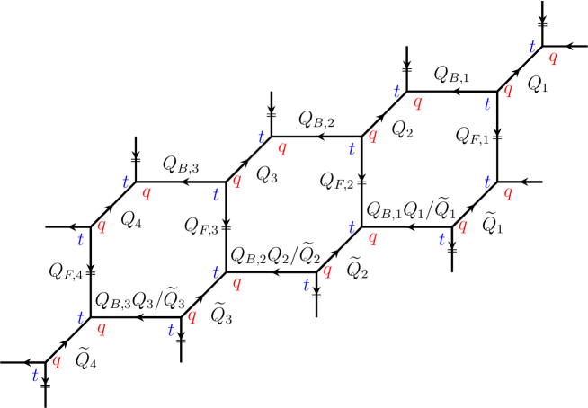
Figure 3: Toric diagram corresponding to the $U(2)^{3}$ gauge theory from Fig. 2.

There is a natural decomposition of the toric diagram depicted on Fig. 3 which leads to the same quiver structure as in Fig. 2 and the Nekrasov expression (9). One should perform the sums over all Young diagrams except those residing on the horizontal edges marked with $Q_{B,i}$, which are related to positions of the vertex operators in the conformal block and the gauge theory couplings $\Lambda_{i}$. In this way one obtains a sum over a chain of pairs of Young diagrams of certain rational factors, which turn out to coincide with $z_{\mathrm{vect},\mathrm{fund},...}$ for $t=q$ (we introduce $t=q^{\beta}$). The resulting expression has exactly the form of Nekrasov function (9). Moreover, each term in the Nekrasov decomposition can now be decomposed into an infinite sum of simpler building blocks $Z^{R}_{AB}$, related to the four-point topological string amplitude on resolved conifold. In the language of CFT this leads to the decomposition

$$\langle\widetilde{\Delta}_{1},\vec{Y}_{1}|V_{\Delta_{2}}(\Lambda_{1})|\widetilde{\Delta}_{2},\vec{Y}_{2}\rangle\sim\sum_{R}Z^{R}_{Y_{1,1}Y_{2,1}}Z^{R}_{Y_{1,2}Y_{2,2}},$$ (12)

and we show that the r.h.s. is nothing but the $q$-deformed version of DF integral expression for the matrix element in the l.h.s.

Another natural decomposition of the toric diagram — cutting along the vertical edges marked with $Q_{F,i}$ (related to Coulomb moduli of the gauge theory and intermediate dimensions in the conformal block) — corresponds to the spectral dual Nekrasov function. The gauge theory origin of this dual description is that in $5d$ instantons are BPS particles as are the gauge bosons. Spectral duality exchanges these two sets of BPS objects and therefore leads to a nontrivial identification between two gauge theories. We will show that the spectral dual decomposition of the toric diagram has a natural interpretation in terms of DF integrals of $q$-CFT — it is the sum featuring in the discrete Jackson integrals, each vertical leg corresponding to a separate integration contour in (1). Therefore, the spectral dual decomposition over horizontal lines of the diagram corresponds to the DF integrals themselves, while the original Nekrasov decomposition is the sum over a complete set of intermediate basis states in the CFT:

$$\mathcal{B}_{k+2}\cdot\mathcal{B}_{U(1)}\sim\sum_{R_{1},\ldots,R_{k}}Z^{R_{1},\ldots,R_{k}}Z^{R_{1},\ldots,R_{k}}$$ (13)

Our goal in this paper is to explain the relation between Eq. (7), Eq. (9), and Fig. 3. We will learn that the identification between conformal block and Nekrasov function requires a nontrivial rewriting of the Vandermonde determinant (which is the product of all-with-all form) into the sum of Nekrasov form (which is of nearest-neighbour form). We first clarify the relation of the toric diagram and the DF integral schematically in the simplest case of the four-point conformal block ($k=2$). Extension to arbitrary $k$ involves an a priori non-trivial star-chain identity, which is in fact the key to understanding DF description of conformal blocks and relies upon the basic properties of representation theory. Another crucial property is Selberg factorization — a mysterious conspiracy between the integrands and integration measure in DF theory, between what is averaged and how it is done. This property guarantees that the averages of certain polynomials over the $q$-Selberg measure factorize into products of linear factors depending on the parameters of the integral. The last mystery is that the elementary building block in the quadrilinear decomposition of conformal blocks, i.e. the topological vertex, is closely related to the modular kernel and therefore to certain knot polynomials.

1.3 Refinement and slicing invariance

The calculation we have just described yields the Nekrasov function of the $5d$ gauge theory with the particular choice of $\Omega$-deformation parameters, i.e. $\epsilon_{1}=-\epsilon_{2}$, or equivalently $t=q$, which corresponds to $c=1$ in CFT. To obtain the partition function in a general $\Omega$-background, one has to use refined topological vertex [17]:

$$C_{ABC}(t,q)=\quad\parbox{56.9055pt}{ \includegraphics[width=56.9055pt]{ref-vertex-crop}}\quad=q^{\frac{||B||^{2}+||C||^{2}}{2}}t^{-\frac{||B^{\mathrm{T}}||^{2}+||C^{\mathrm{T}}||^{2}}{2}}M^{(q,t)}_{C}\left(t^{-\rho}\right)\times\\ \times\sum_{D}\left(\frac{q}{t}\right)^{\frac{|D|+|A|-|B|}{2}}\chi_{A^{\mathrm{T}}/D}\left(q^{-C}t^{-\rho}\right)\chi_{B/D}\left(t^{-C^{\mathrm{T}}}q^{-\rho}\right),$$ (14)

where $||A||^{2}=\sum_{i}A_{i}^{2}$ and $M_{C}^{(q,t)}(x)$ are Macdonald polynomials. Notice that one of the legs in the diagram is marked with a double stroke and the other two bear $t$ and $q$ labels on them. This is to indicate the right order of the indices and arguments of the refined vertex, which depends on two deformation parameters and is not cyclically symmetric as was the case for $t=q$.

The calculations generally get more technically involved, though the strategy remains the same. The only essentially new feature in this case is the naive loss of rotation symmetry of the diagram: the vertical and horizontal lines are no longer equivalent. However, it turns out that the symmetry in fact survives even for general $t$ and $q$, though the individual vertices and propagators are not symmetric. This statement came to be known as the slicing invariance hypothesis. For toric geometries, which we consider, slicing invariance is also equivalent to spectral duality [21] of the corresponding Nekrasov partition functions, since the two sides of the duality are related to the $\frac{\pi}{2}$ rotation of the whole toric diagram including the choice of preferred direction. We look at different choices of “slicing” of the toric diagram and relate them to different choices of the basis in conformal field theory. One slicing direction corresponds to the “naive” basis of Schur polynomials $\chi_{A}$, the other — to the basis of generalized Macdonald polynomials $M_{AB}$. The first set of polynomials does not have factorized $q$-Selberg averages and does not reproduce the Nekrasov factors, while our calculations indicate that the second one does. Schematically

$$\left\langle\sum_{E,F}\chi_{A/E}\chi_{C/E}\chi_{B/F}\chi_{D/F}\right\rangle\neq\left\langle\sum_{E,F}M_{AB/EF}M_{CD/EF}\right\rangle\sim\frac{z_{\mathrm{bifund}}\left([A,B],[C,D]\right)}{(z_{\mathrm{vect}}([A,B])z_{\mathrm{vect}}([C,D]))^{1/2}}.$$ (15)

The last equality is a new generalization of the “factorization of averages” type of identities, studied in [25], [20].

We investigate the connection between the two sets of polynomials and introduce generalized Kostka functions $K_{AB}^{CD}$ transforming one basis into the other:

$$M_{AB}=\sum_{CD}K_{AB}^{CD}\chi_{C}\chi_{D}.$$ (16)

These functions are effectively performing the $\frac{\pi}{2}$ rotation of preferred direction. In more algebraic terms they are related to the abelianization map [29] acting on the basis in $K$-theory of instanton moduli space.

The paper is partitioned into a set of sections with increasing level of detail and complexity. After reviewing the basic steps of the construction at the simplified level in sec. 2 we fill in the details and provide full-fledged formulas for the unrefined case in sec. 3. We then treat the refined case in sec. 4. We provide a summary and point out future directions in sec. 5.

2 Basic steps

In this section we introduce our approach to Dotsenko–Fateev integral expansion without $q$-deformation. We consider first the most simple example of four-point conformal block and show how decompose the integrand in terms of Schur polynomials. Next we consider the multi-point block and observe that a nontrivial star-chain duality is required in this case. We demonstrate this duality explicitly using skew Schur functions.

2.1 Four point conformal block, no $q$-deformation

In the case of four-point conformal block there are two contours of integration: $\mathcal{C}_{1}$ stretching from $0$ to $1$ and $\mathcal{C}_{\Lambda}$ stretching from $0$ to $\Lambda^{-1}$. Therefore, the variables in the integration in Eq. (1) are divided into two groups: $x_{i}$ and $y_{i}$ and the inter-screening pairings are decomposed into a product

$$\Delta(z)^{2\beta}\to\Delta(x)^{2\beta}\times\Delta(y)^{2\beta}\times\underbrace{\prod_{i=1}^{N_{1}}\prod_{j=1}^{N_{2}}\left(1-\frac{x_{i}}{y_{j}}\right)^{2\beta}}_{\text{cross term}}.$$

The vertex operator contributions also decompose into a product of two factors:

$$\prod_{i=1}^{N_{1}+N_{2}}(1-z_{i})^{v_{1}} \to\prod_{i=1}^{N_{1}}(1-x_{i})^{v_{1}}\times\underbrace{\prod_{i=1}^{N_{2}}(1-y_{i}^{-1})^{v_{1}}}_{\text{cross term}},$$

$$\prod_{i=1}^{N_{1}+N_{2}}(1-\Lambda z_{i})^{v_{2}} \to\prod_{i=1}^{N_{2}}(1-\Lambda y_{i})^{v_{2}}\times\underbrace{\prod_{i=1}^{N_{1}}(1-\Lambda x_{i})^{v_{2}}}_{\text{cross term}}.$$

Making a change of variables $y_{i}\to\frac{y_{i}}{\Lambda}$ we can write the cross terms which we denote by $\mu_{\mathrm{cross}}(x,y)$ as follows:

$$\mu_{\mathrm{cross}}(x,y)=\prod_{i=1}^{N_{1}}\prod_{j=1}^{N_{2}}\left(1-\Lambda\frac{x_{i}}{y_{j}}\right)^{2\beta}\prod_{i=1}^{N_{2}}\left(1-\frac{\Lambda}{y_{i}}\right)^{v_{1}}\prod_{i=1}^{N_{1}}(1-\Lambda x_{i})^{v_{2}}$$

Employing the Cauchy completeness identity (4) we get the expansion of the cross contributions in terms of Jack polynomials:

$$\mu(x,y)=\exp\left(-\sum_{n\geq 1}\frac{\Lambda^{n}}{n}(2\beta p_{n}q_{-n}+v_{1}q_{-n}+p_{n}v_{2})\right)=\\ =\sum_{Y_{1},Y_{2}}\Lambda^{|Y_{1}|+|Y_{2}|}J_{Y_{1}}(p_{n})J_{Y_{2}}\left(-p_{n}-\frac{v_{1}}{\beta}\right)J_{Y_{1}}\left(-q_{-n}-\frac{v_{2}}{\beta}\right)J_{Y_{2}}(q_{-n}),$$ (17)

where $p_{n}=\sum_{i=1}^{N_{1}}x_{i}^{n}$, $q_{n}=\sum_{i=1}^{N_{2}}y_{i}^{n}$.

After this decomposition the DF integral becomes the double Selberg average of Jack polynomials

$$\mathcal{B}_{4}=\sum_{Y_{1},Y_{2}}\Lambda^{|Y_{1}|+|Y_{2}|}\left\langle J_{Y_{1}}(p_{n})J_{Y_{2}}\left(-p_{n}-\frac{v_{1}}{\beta}\right)\right\rangle_{u_{1},v_{1},N_{1},\beta}\left\langle J_{Y_{1}}\left(-q_{-n}-\frac{v_{2}}{\beta}\right)J_{Y_{2}}(q_{-n})\right\rangle_{u_{2},v_{2},N_{2},\beta}$$ (18)

where the averages are taken with respect to the measure $\mu(x|u_{a},v_{a},N_{a},\beta)=\Delta^{2\beta}(x)\prod_{i=1}^{N_{a}}\left(x_{i}^{u_{a}}(1-x_{i})^{v_{a}}_{\phantom{i}}\right)$. For general $\beta$ the averages (17) do not give the Nekrasov expansion of the conformal block (a more refined basis of generalized Jack functions $J_{AB}$ depending on a pair of diagrams is required [25]). However, for the special case $\beta=1$ when Jack polynomials turn into Schur functions the structure of Nekrasov sum is indeed reproduced [22].

Thus, from the four-point case without $q$-deformation we learn that decomposing the inter-screening pairings in the DF integral in terms of characters and then taking the Selberg averages produces Nekrasov representation of the conformal block. We now move to the multi-point case where the star-chain duality is required to obtain Nekrasov decomposition.

2.2 Multi-point case. Star-chain duality

2.2.1 An apparent paradox

If one approaches the multipoint case in a naive way one arrives at what seems to be a paradox. The DF representation contains a product of all pairings between screening operators, i.e. an expression of the form

$$\prod_{a<b}\left(1-\frac{x_{i}^{a}}{x_{j}^{b}}\right)^{2\beta}.$$ (19)

However, the gauge theory corresponding to the multipoint comb-like conformal block is a linear quiver of the form depicted in Fig. 2, and its Nekrasov partition function contains only the nearest neighbour pairings:

$$\prod_{a}z_{\mathrm{bifund}}(Y_{a},Y_{a+1})$$ (20)

Thus the multilinear decomposition of the DF integral should also have the nearest-neighbor structure. In the four-point case there are only two term in the product, so that all-with-all (star) type interaction is the same as nearest-neighbour (chain) one. But how can one decompose the multi-point product (19) into a sum of nearest-neighbour products, how can star become equivalent to a chain?

2.2.2 Skew characters

The resolution of the paradox is technically based on the properties of skew characters,

$$\chi_{{}_{A/W}}\stackrel{{\scriptstyle\mathrm{def}}}{{=}}\sum_{B}c^{A}_{{}_{BW}}\chi_{{}_{B}}$$ (21)

where $c^{A}_{BC}$ are the Littlewood-Richardson coefficients, describing multiplication of representations:

$$\chi_{{}_{B}}\chi_{{}_{C}}=\sum_{A}c^{A}_{{}_{BC}}\chi_{{}_{A}}$$ (22)

Directly from the definitions,

$$\sum_{A}\chi_{A}[x]\chi_{A/W}[y]=\sum_{A,B}c^{A}_{BW}\chi_{A}[x]\chi_{B}[y]=\chi_{W}[x]\cdot\sum_{B}\chi_{B}[x]\chi_{B}[y]=\chi_{W}[x]\cdot\prod_{i,j}(1-x_{i}y_{j})^{-1}$$ (23)

Moreover, this is straightforwardly generalized to

$$\boxed{\sum_{A}\chi_{A}\Big{(}p_{n}(x^{(1)})+\ldots+p_{n}(x^{(m)})\Big{)}\cdot\chi_{A/W}[y]=\chi_{W}\Big{(}p_{n}(x^{(1)})+\ldots+p_{n}(x^{(m)})\Big{)}\cdot\prod_{a=1}^{m}\prod_{i,j}(1-x_{i}^{(m)}y_{j})^{-1}}$$ (24)

Similarly,

$$\sum_{W}\chi_{W}[x]\chi_{A/W}[y]=\sum_{B,W}c^{A}_{BW}\chi_{B}[y]\chi_{W}[x]$$ (25)

Convolution with $\chi_{A}[z]$ gives:

$$\sum_{A}\chi_{A}[z]\left(\sum_{W}\chi_{W}[x]\chi_{A/W}[y]\right)=\sum_{B,W}\left(\sum_{A}c^{A}_{BW}\chi_{A}[z]\right)\chi_{B}[y]\chi_{W}[x]=\left(\sum_{B}\chi_{B}[z]\chi_{B}[y]\right)\left(\sum_{W}\chi_{W}[z]\chi_{W}[x]\right)$$

$$=\exp\left\{\sum_{k}\frac{1}{k}p_{k}(z)\Big{(}p_{k}(x)+p_{k}(y)\Big{)}\right\}=\sum_{A}\chi_{A}[z]\chi_{A}\Big{(}p_{n}(x)+p_{n}(y)\Big{)}$$ (26)

i.e.

$$\boxed{\sum_{W}\chi_{W}[x]\chi_{A/W}[y]=\chi_{A}\Big{(}p(x)+p(y)\Big{)}}$$ (27)

At $x=y$ we can apply (22) to the l.h.s. to get a doubling rule

$$\chi_{{}_{A}}(2p_{n})=\sum_{B}\Big{(}\sum_{V,W}C^{A}_{{}_{VW}}C^{B}_{{}_{VW}}\Big{)}\cdot\chi_{{}_{B}}(p_{n})$$ (28)

e.g. $\chi_{{}_{[1]}}(2p_{n})=2\chi_{{}_{[1]}}(p_{n}),\ \ \chi_{{}_{[2]}}(2p_{n})=3\chi_{{}_{[2]}}(p_{n})+\chi_{{}_{[11]}}(p_{n}),\ \ \chi_{{}_{[11]}}(2p_{n})=\chi_{{}_{[2]}}(p_{n})+3\chi_{{}_{[11]}}(p_{n}),\ \ \chi_{{}_{[3]}}(2p_{n})=4\chi_{{}_{[3]}}(p_{n})+2\chi_{{}_{[21]}}(p_{n}),\ \ \chi_{{}_{[21]}}(2p_{n})=2\chi_{{}_{[3]}}(p_{n})+6\chi_{{}_{[21]}}(p_{n})+2\chi_{{}_{[111]}}(p_{n}),\ \ \chi_{{}_{[111]}}(2p_{n})=2\chi_{{}_{[21]}}(p_{n})+4\chi_{{}_{[111]}}(p_{n}),\ \ldots$ which can be further promoted to tripling, quadrupling and higher multiplication formulas.

2.2.3 Resolution of the star/chain problem. From chain to star. Bifundamental kernel

We claim that the chain of skew characters indeed reproduces the star-like structure of the DF integrand. The basic building block of the chain decomposition is the bifundamental kernel

$$N_{AB}[y]=\sum_{C}\chi_{A/C}^{*}[y]\chi_{B/C}[y],$$ (29)

where $\chi_{Y}^{*}[x]=\chi_{Y}[-p_{n}(x^{-1})]$. Two such kernels, averaged over the Selberg measure like $\langle N_{AB}[y]N_{CD}[y]\rangle$, correspond to a single bifundamental field in Nekrasov partition function of the gauge theory depending on two pairs of diagrams $(A,B)$ and $(C,D)$. Observe that $N_{\varnothing A}[x]=\chi_{A}[x]$, $N_{A\varnothing}[x]=\chi_{A}^{*}[x]$.

We start with the case of five-point conformal block. Using the identities from the previous section, we can rewrite the chain answer into the Dotsenko-Fateev (star) form:

$$\sum_{Y_{1},Y_{2}}N_{\varnothing Y_{1}}[x]N_{Y_{1}Y_{2}}[y]N_{Y_{2}\varnothing}[z]=\\ =\sum_{Y_{1},Y_{2},W}\chi_{{}_{Y_{1}}}[x]\chi_{{}_{Y_{1}/W}}^{*}[y]\chi_{{}_{Y_{2}/W}}[y]\chi_{{}_{Y_{2}}}^{*}[z]=\prod_{i,j}\left(1-\frac{x_{i}}{y_{j}}\right)\sum_{Y_{2},W}\chi_{{}_{W}}[x]\chi_{{}_{Y_{2}/W}}[y]\chi_{{}_{Y_{2}}}^{*}[z]=\\ =\prod_{i,j}\left(1-\frac{x_{i}}{y_{j}}\right)\sum_{{}_{Y_{2}}}\chi_{{}_{Y_{2}}}\Big{(}p_{n}(x)+p_{n}(y)\Big{)}\chi_{{}_{Y_{2}}}^{*}[z]=\prod_{i,j}\left(1-\frac{x_{i}}{y_{j}}\right)\prod_{i,j}\left(1-\frac{y_{i}}{z_{j}}\right)\prod_{i,j}\left(1-\frac{x_{i}}{z_{j}}\right)$$ (30)

where $\chi^{*}[y]=\chi[-p_{n}(y^{-1})]=\chi[-p_{-n}(y)]$.

Similarly for a general $(k+2)$-point conformal block:

$$\sum_{Y_{a}}N_{\varnothing Y_{1}}[x]\left(\prod_{a=1}^{k-2}N_{Y_{a}Y_{a+1}}[y_{a}]\right)N_{Y_{k-1}\varnothing}[z]=\sum_{Y_{a},W_{a}}\chi_{{}_{Y_{1}}}[x]\left(\prod_{a=1}^{k-2}\chi_{{}_{Y_{a}/W_{a}}}^{*}[y_{a}]\chi_{{}_{Y_{a+1}/W_{a}}}[y_{a}]\right)\chi_{{}_{Y_{k-1}}}^{*}[z]=\\ =\prod_{i,j}\left(1-\frac{x_{i}}{y_{1j}}\right)\sum_{Y_{a},W_{a}}\chi_{{}_{Y_{2}}}\Big{(}p_{n}[x]+p_{n}[y_{1}]\Big{)}\left(\prod_{a=2}^{k-2}\chi_{{}_{Y_{a}/W_{a}}}^{*}[y_{a}]\chi_{{}_{Y_{a+1}/W_{a}}}[y_{a}]\right)\chi_{{}_{Y_{k-1}}}^{*}[z]=\\ \!\!\!\!\!\!\!=\prod_{i,j}\left(1-\frac{x_{i}}{y_{1j}}\right)\left(1-\frac{x_{i}}{y_{2j}}\right)\left(1-\frac{y_{1i}}{y_{2j}}\right)\sum_{Y_{a},W_{a}}\chi_{{}_{Y_{3}}}\Big{(}p_{n}[x]+p_{n}[y_{1}]+p_{n}[y_{2}]\Big{)}\left(\prod_{a=3}^{k-2}\chi_{{}_{Y_{a}/W_{a}}}^{*}[y_{a}]\chi_{{}_{Y_{a+1}/W_{a}}}[y_{a}]\right)\chi_{{}_{Y_{k-1}}}^{*}[z]=\\ =\ \ldots\ =\prod_{i,j}\left\{\left(1-\frac{x_{i}}{z_{j}}\right)\prod_{a}\left(1-\frac{x_{i}}{y_{aj}}\right)\prod_{a<b}\left(1-\frac{y_{ai}}{y_{bj}}\right)\prod_{a}\left(1-\frac{y_{ai}}{z_{j}}\right)\right\}.$$ (31)

2.2.4 From star to chain

Inverting this short derivation, we see that it is an iteration of the two-step procedure, which starts from $m=k-1$ with $F_{k-1}[Y]=\chi_{{}_{Y}}^{*}[z]$ and ends at $m=2$ with $x=y_{0}$.

In obvious notation:

$$\sum_{Y_{m}}F_{m}\{Y_{m}\}\!\cdot\!\chi_{{}_{Y_{m}}}[y_{0},y_{1},\ldots,y_{m-1}]=\sum_{Y_{m},W_{m-1}}\underline{F_{m}\{Y_{m}\}\cdot\chi_{{}_{Y_{m}/W_{m-1}}}[y_{m-1}]}\cdot\chi_{{}_{W_{m-1}}}[y_{0},\ldots,y_{m-2}]$$ (32)

Underlined piece goes directly to the chain-side of the identity, while the remaining multi-character is combined with the next product

$$\sum_{Z_{m-1}}\chi_{{}_{Z_{m-1}}}^{*}[y_{m-1}]\cdot\chi_{{}_{Z_{m-1}}}[y_{0},\ldots,y_{m-2}]$$ (33)

Since, whatever are the sets $u$ and $w$,

$$\sum_{Z}\chi_{{}_{Z}}[u]\chi_{{}_{Z}}[w]\chi_{{}_{W}}[w]=\sum_{Z,Y}C_{{}_{ZW}}^{Y}\chi_{{}_{Z}}[u]\chi_{{}_{Y}}[w]=\sum_{Y}\chi_{{}_{Y/W}}[u]\chi_{{}_{Y}}[w]$$ (34)

we get:

$$\sum_{Y_{m-1}}\ \underbrace{\sum_{Y_{m},W_{m-1}}F_{m}\{Y_{m}\}\cdot\chi_{{}_{Y_{m}/W_{m-1}}}[y_{m-1}]\ \chi^{*}_{{}_{Y_{m-1}/W_{m-1}}}[y_{m-1}]}_{F_{m-1}\{Y_{m-1}\}}\ \cdot\ \chi_{{}_{Y_{m-1}}}[y_{0},\ldots,y_{m-2}]=\\ =\sum_{Y_{m-1}}F_{m-1}\{Y_{m-1}\}\cdot\chi_{{}_{Y_{m-1}}}[y_{0},y_{1},\ldots,y_{m-2}]$$ (35)

and we are ready for the next iteration.

At $k=3$ this can be pictorially represented as

Dots here stand for characters, and arrows point from $\chi$ to $\chi^{*}$. At two steps we apply (22) to substitute the encycled product of characters by a single character. Note that only dots at the same place which are both either starting or end-points of the arrows can be merged in this way.

Likewise at $k=4$:

and at $k=5$:

The main secret behind this derivation is that the structure constants in (22) are always the same — do not depend on the number of “Miwa variables” $y_{i}$ in $\chi[y_{0},\ldots,y_{m}]$ — what allows to merge entire collections of points and parallel arrows in above examples. This conspiracy between characters and the structure constants adds to associativity of multiplication and together they provide the star-chain equivalence.

2.3 Factorization of Selberg averages

The “chain” decomposition of DF integrals (31) is also tied with the structure of the Selberg averages. More concretely, the averages of the bifundamental kernels (29) are given by the factorized formulas:

$$\left\langle N_{AC}[x]N_{BD}[-p_{n}(x)-v]\right\rangle_{u,v,N,\beta=1}=(-1)^{|B|+|D|}\frac{z_{\mathrm{bifund}}^{4d}\left([A,B],[C,D],u/2+v/2+N,u/2,-v/2\right)}{C_{A}^{4d}C_{B}^{4d}C_{C}^{4d}C_{D}^{4d}G_{AB}^{4d}(u+v+2N)G_{CD}^{4d}(u)},$$ (36)

where

$$C_{A}^{4d}=\prod_{(i,j)\in A}\left(\mathrm{Arm}_{A}(i,j)+\mathrm{Leg}_{A}(i,j)+1\right),$$ (37)

$$G_{AB}^{4d}(x)=\prod_{(i,j)\in A}\left(x+A_{i}-j+B^{\mathrm{T}}_{j}-i+1\right)\prod_{(i,j)\in B}\left(x-B_{i}+j-1-A^{\mathrm{T}}_{j}+i\right).$$ (38)

$$z_{\mathrm{bifund}}^{4d}\left(\vec{A},\vec{B},\vec{a},\vec{b},m\right)=\prod_{i,j=1}^{2}G^{4d}_{A_{i}B_{j}}(a_{i}-b_{j}-m)$$ (39)

and $\vec{a}=(a,-a)$, $\vec{b}=(b,-b)$. This factorization means that expansion of the DF integrand in terms of the bifundamental kernels $N_{AB}$ indeed reproduces the Nekrasov decomposition. In the next section we will compute the $q$-deformed averages and show how to decompose them even further to obtain topological vertices.

3 Complete formulas for $t=q$

In this section we flesh out the basic formulas introduced in the previous section and incorporate $q$-deformation into our framework. After $q$-deformation, we obtain the natural identification of DF integral decompositions with topological vertices. We start with especially symmetric example of the four-point conformal block of $q$-Virasoro algebra and then consider multi-point blocks. We calculate $q$-deformed Selberg averages of the skew characters and identify the elements of the multilinear decomposition with topological string amplitudes.

3.1 Four point conformal block ($t=q$)

The origin of the quadrilinear expansion of the four point conformal block is straightforward to see: two diagrams come from the character decomposition and two more represent the two integration contours in the DF integral (which becomes a sum in the $q$-deformed case [20]). The corresponding toric diagram is depicted in Fig. 4 and the four diagrams are denoted by $A$, $B$, $R_{+}$ and $R_{-}$.

The DF representation is given by the sum over DF poles labelled by two partitions $R_{\pm}$:

$$\mathcal{B}_{4}=\sum_{R_{\pm}}\mu(x_{R_{+}})\mu_{\mathrm{cross}}(x_{R_{+}},x_{R_{-}})\mu(x_{R_{+}}).$$ (40)

The contribution of the $q$-Selberg measure $\mu(x|u,v,N,q,q)=\Delta(x)\prod_{i=1}^{N}\left(x_{i}^{u}\prod_{k=0}^{v-1}(1-q^{k}x_{i})\right)$ can be evaluated explicitly and is written as follows:

$$\frac{\mu(x_{R}|u,v,N,q,q)}{\mu(x_{\varnothing}|u,v,N,q,q)}=q^{|R|(2N+u+v-1)}\chi_{R}^{(N)}(q^{\rho})\chi_{R}^{(N+v)}(q^{\rho})=q^{|R|(u-1)}\chi_{R}^{(N)}(q^{-\rho})\chi_{R}^{(N+v)}(q^{-\rho}),$$ (41)

$$x_{R,i}=q^{R_{i}-i+N+1},$$ (42)

and $\chi_{A}^{(N)}(x)$ denotes Schur polynomial in $N$ variables $x_{i}$. The cross contribution reads

$$\mu_{\mathrm{cross}}(x,y)=\prod_{i=1}^{N_{+}}\prod_{j=1}^{N_{-}}\left(1-\Lambda\frac{x_{i}}{y_{j}}\right)^{2}\prod_{j=1}^{N_{-}}\prod_{n=0}^{v_{+}-1}\left(1-\Lambda q^{-n}\frac{1}{y_{j}}\right)\prod_{i=1}^{N_{+}}\prod_{l=0}^{v_{-}-1}\left(1-\Lambda q^{l}x_{i}\right)=\\ =\exp\left\{\sum_{n\geq 1}\frac{\Lambda^{n}}{n}\left[\left(p_{n}+\frac{1-q^{-nv_{+}}}{1-q^{-n}}\right)(-q_{-n})+p_{n}\left(-q_{-n}-\frac{1-q^{nv_{-}}}{1-q^{n}}\right)\right]\right\}=\\ =\sum_{A,B}\left(-\Lambda q^{N_{+}-N_{-}}\right)^{|A|+|B|}\chi_{A}\left(q^{-(N_{+}+1/2)n}p_{n}+\sum_{i=N_{+}+1}^{N_{+}+v_{+}}q^{n(1/2-i)}\right)\chi_{B}\left(q^{-(N_{+}+1/2)n}p_{n}\right)\times\\ \times\chi_{A^{\mathrm{T}}}\left(q^{n(N_{-}+1/2)}q_{-n}\right)\chi_{B^{\mathrm{T}}}\left(q^{(N_{-}+1/2)n}q_{-n}+\sum_{i=N_{-}+1}^{N_{-}+v_{-}}q^{-n(1/2-i)}\right),$$ (43)

where $p_{n}=\sum_{i=1}^{N_{+}}x_{i}^{n}$, $q_{n}=\sum_{j=1}^{N_{-}}y_{j}^{n}$ and we have employed the Cauchy identity and the identity $\chi_{A}(-p_{n})=(-1)^{|A|}\chi_{A^{\mathrm{T}}}(p_{n})$. Collecting all the contributions one obtains

$$\mathcal{B}_{4}=\mu(x_{\varnothing}|u_{+},v_{+},N_{+})\,\mu(x_{\varnothing}|u_{-},v_{-},N_{-})\times\\ \times\sum_{R_{+},R_{-}}\sum_{A,B}\left(-\Lambda q^{N_{+}-N_{-}}\right)^{|A|+|B|}q^{|R_{+}|(u_{+}+v_{+}+2N_{+}-1)+|R_{-}|(u_{-}+v_{-}+2N_{-}-1)}\chi_{R_{+}}^{(N_{+})}(q^{\rho})\chi_{R_{+}}^{(N_{+}+v_{+})}(q^{\rho})\times\\ \times\chi_{R_{-}}^{(N_{-})}(q^{\rho})\chi_{R_{-}}^{(N_{-}+v_{-})}(q^{\rho})\chi_{B}^{(N_{+})}(q^{R_{+}+\rho})\chi_{A^{\mathrm{T}}}^{(N_{-})}(q^{-R_{-}-\rho})\chi_{A}^{(N_{+}+v_{+})}(q^{R_{+}+\rho})\chi_{B^{\mathrm{T}}}^{(N_{-}+v_{-})}(q^{-R_{-}-\rho}).$$ (44)

Figure 4: Toric diagram corresponding to the four-point $q$-deformed conformal block and $5d$ $U(2)$ gauge theory with four fundamentals.

Using the identities

$$\chi_{R}^{(N)}(q^{\rho})=(-1)^{|R|}q^{-N|R|}\chi_{R^{\mathrm{T}}}^{(-N)}(q^{\rho}),\qquad\qquad\chi_{A}^{(N)}(q^{-R-\rho})=(-1)^{|A|}\chi_{A^{\mathrm{T}}}^{(-N)}(q^{R^{\mathrm{T}}+\rho})$$

one gets

$$\mathcal{B}_{4}=\mu(x_{\varnothing}|u_{+},v_{+},N_{+})\,\mu(x_{\varnothing}|u_{-},v_{-},N_{-})\sum_{R_{+},R_{-}}\sum_{A,B}\left(\Lambda q^{N_{+}-N_{-}}\right)^{|A|+|B|}q^{|R_{+}|(u_{+}+v_{+}+2N_{+}-1)+|R_{-}|(u_{-}-1)}\times\\ \times S_{R_{+}B}(q^{-N_{+}})S_{AR_{-}^{\mathrm{T}}}(q^{N_{-}})S_{R_{-}^{\mathrm{T}}B}(q^{N_{-}+v_{-}})S_{AR_{+}}(q^{-N_{+}-v_{+}}),$$ (45)

where

$$S_{AB}(Q)=\chi_{A}(p_{n}(q^{\rho})-p_{n}(Qq^{\rho}))\chi_{B}(p_{n}(q^{A+\rho})-p_{n}(Qq^{\rho}))$$ (46)

is the open topological string amplitude for the resolved conifold. Pictorially $S_{AB}(Q)$ is given by one corner of the toric diagram from Fig. 4. It is also equal to the Chern-Simons (or WZW) $S$-matrix.

Using the AGT relations (86) one immediately obtains the identification between the Kähler parameters of the toric Calabi-Yau, CFT and the gauge theory parameters:

$$Q_{B}=\Lambda q^{N_{+}-N_{-}}=\Lambda q^{-2a+m_{2}^{+}-m_{2}^{-}},$$

$$Q_{F}=q^{2N_{+}+u_{+}+v_{+}-1}=q^{u_{-}-1}=q^{-2a-1},$$

$$Q_{1}^{+}=q^{-N_{+}-v_{+}}=q^{a+m_{1}^{+}},\quad Q_{2}^{+}=q^{-N_{+}}=q^{a-m_{2}^{+}},$$

$$Q_{1}^{-}=q^{N_{-}}=q^{a+m_{2}^{-}},\quad Q_{2}^{-}=q^{N_{-}+v_{-}}=q^{a-m_{1}^{-}}.$$

Let us state once more the result for the four-point $q$-deformed conformal block for $t=q$. This block can be simultaneously decomposed in two ways: DF integral and the decomposition in terms of the complete basis of states. Using the simplest choice of basis states (Schur functions) one gets a symmetric quadrilinear decomposition in terms of characters. Moreover, this decomposition is naturally identified with the corresponding topological string amplitude, computed using the topological vertex technique. We now move on to describe the multipoint case.

3.2 Multipoint ($t=q$)

In section 2.2.3 we understood the star-chain transformation for ordinary DF integrals. The $q$-deformed case goes along the same lines. Also, as in the four-point case above, we obtain a natural interpretation of the objects featuring in the decomposition from the point of view of the topological strings.

Using the star-chain relation we rewrite the Vandermonde measure in the multipoint DF integral as a sum over chains of skew Schur functions. We consider the corresponding expansion of the $k$-point DF integral in terms of $k$ $q$-deformed Selberg averages of skew Schur functions (cf. Eq. (31)):

$$\mathcal{B}_{k+2}\mathcal{B}_{U(1)}=\sum_{\{\vec{Y}_{a}\}}\prod_{a=1}^{k}\Lambda_{a}^{|\vec{Y}_{a}|}\Biggl{\langle}N_{Y_{a-1,1}Y_{a,1}}[x]N_{Y_{a-1,2}Y_{a,2}}\left[-p_{n}-\frac{1-q^{-nv_{a}}}{1-q^{-n}}\right]\Biggr{\rangle}_{u_{a},v_{a},N_{a},q,q}$$ (47)

where $\langle\ldots\rangle_{u_{a},v_{a},N_{a},q,q}$ denotes the $q$-Selberg average with the corresponding parameters and $\vec{Y}_{0}=\vec{Y}_{k}=(\varnothing,\varnothing)$. Each average depends on two pairs of Young diagrams $\vec{Y}_{a-1}$, $\vec{Y}_{a}$ and corresponds to the element of the toric diagram depicted on Fig. 5. Notice that a certain $U(1)$ factor appears in the left hand site. It can be nicely eliminated in the four-point case, though not for higher multipoints.

In the next section we show that each average in Eq. (47) indeed reproduces the bifundamental part of the Nekrasov function. The whole sum thus becomes the Nekrasov function for linear quiver gauge theory, of the form depicted in Fig. 2.

$$Z\left(\left.\begin{smallmatrix}&\varnothing&\\ Y_{a,1}&&Y_{a-1,1}\\ Y_{a,2}&&Y_{a-1,2}\\ &\varnothing&\end{smallmatrix}\right|Q_{1},Q_{2},Q_{F},q,q\right)\quad=\quad\parbox{99.58464pt}{\includegraphics[width=99.58464pt]{bifund-crop} }$$

Figure 5: Toric diagram corresponding to bifundamental field in the Nekrasov function. It is also equal to $q$-deformed Selberg average of two bifundamental kernels as in Eq. (47).

3.3 Factorization of averages

Let us check that the DF averages of the bifundamental kernel $N_{AB}[x]$ indeed factorizes. To do it we use the loop equations, which are given in Appendix B. We obtain a formula for the average of four Schur polynomials:

$$\left\langle N_{AC}[x]N_{BD}\left[-p_{n}(x)-\frac{1-q^{-nv}}{1-q^{-n}}\right]\right\rangle_{u,v,N,q,q}=\\ =q^{(1-v)(|C|-|A|+|D|-|B|)}\left\langle N_{AC}[x^{-1}]N_{BD}\left[-p_{n}(x^{-1})-\frac{1-q^{nv}}{1-q^{n}}\right]\right\rangle_{-u-v-2N,v,N,q,q}=\\ =(-1)^{|B|+|D|}q^{-u|B|-(2N+u)|C|+v|D|}q^{\kappa_{ABCD}}\frac{z_{\mathrm{bifund}}^{(q,q)}\left([A,B],[C,D],q^{-u/2},q^{-u/2-v/2-N},q^{v/2}\right)}{C^{\prime}_{A}(q,q)C^{\prime}_{B}(q,q)C^{\prime}_{C}(q,q)C^{\prime}_{D}(q,q)G_{AB}^{(q,q)}(q^{-u})G_{CD}^{(q,q)}(q^{-u-v-2N})},$$ (48)

where

$$C^{\prime}_{A}(q,t)=\prod_{(i,j)\in A}\left(1-q^{\mathrm{Arm}_{A}(i,j)}t^{\mathrm{Leg}_{A}(i,j)+1}\right),$$ (49)

$$\kappa_{ABCD}=-\kappa_{B}/2+\kappa_{C}/2+\sum_{(i,j)\in A}(i-1)+\sum_{(i,j)\in B}(i-1)+\sum_{(i,j)\in C}j+\sum_{(i,j)\in D}j$$ (50)

$$\kappa_{A}=2\sum_{(i,j)\in A}(j-i)$$ (51)

and the definition of $G_{AB}^{(q,t)}$ and $z_{\mathrm{bifund}}^{(q,t)}$ are collected in Appendix A. This indeed proves that the average of four Schur polynomials gives the bifundamental Nekrasov contribution.

3.4 Identification with topological strings

We would like to further decompose the $q$-Selberg average in Eq. (48) to observe the structure of the corresponding topological string amplitude from Fig. 5. Notice that each average contains a product of two bifundamental kernels $N_{AB}[x]$. This corresponds to the product of two four-point functions each having the form:

$$Z\left(\left.\begin{smallmatrix}&\varnothing&\\ C&&A\\ &R^{\mathrm{T}}&\end{smallmatrix}\right|Q_{2},q,q\right)=\quad\parbox{79.6678pt}{\includegraphics[width=79.6678pt]{conifold-ARC-unref-crop}}\quad=\sum_{W}(-Q_{2})^{|W|}C_{A^{\mathrm{T}}W^{\mathrm{T}}\varnothing}(q)C_{CWR^{\mathrm{T}}}(q)=\\ =Z\left(\left.\begin{smallmatrix}&\varnothing&\\ \varnothing&&\varnothing\\ &\varnothing&\end{smallmatrix}\right|Q_{2},q,q\right)q^{\frac{\kappa_{C}-\kappa_{A}}{2}}(-Q_{2})^{|C|}(-1)^{|R|}\chi_{R}^{(N)}(q^{-\rho})N_{AC}^{(N)}\left[q^{-R-\rho}\right],$$ (52)

where $Q_{2}=q^{N}$. Recall the expression for the $q$-deformed Selberg measure (41), which consists of two Schur polynomials. The product of two four-point amplitudes (52) therefore gives exactly the product of $q$-Selberg measure with two bifundamental kernels as in the average (47). More explicitly, gluing two amplitudes (52) one obtains the amplitude from Fig. 5, which is given by:

$$Z\left(\left.\begin{smallmatrix}&\varnothing&\\ C&&A\\ D&&B\\ &\varnothing&\end{smallmatrix}\right|Q_{1},Q_{2},Q_{F},q,t\right)=\sum_{R}(-Q_{F})^{|R|}Z\left(\left.\begin{smallmatrix}&\varnothing&\\ C&&A\\ &R^{\mathrm{T}}&\end{smallmatrix}\right|Q_{2},q,q\right)Z\left(\left.\begin{smallmatrix}&R^{\mathrm{T}}&\\ D&&B\\ &\varnothing&\end{smallmatrix}\right|Q_{1},q,q\right)=\\ =Z\left(\left.\begin{smallmatrix}&\varnothing&\\ \varnothing&&\varnothing\\ &\varnothing&\end{smallmatrix}\right|Q_{1},q,q\right)Z\left(\left.\begin{smallmatrix}&\varnothing&\\ \varnothing&&\varnothing\\ &\varnothing&\end{smallmatrix}\right|Q_{2},q,q\right)q^{\frac{\kappa_{C}-\kappa_{A}+\kappa_{D}-\kappa_{B}}{2}}(-Q_{1})^{|C|}(-Q_{2})^{|D|}\times\\ \times\sum_{R}(-Q_{F})^{|R|}s_{R}^{(N)}(q^{-\rho})s_{R^{\mathrm{T}}}^{(-N-v)}(q^{-\rho})N_{AC}^{(N)}\left[q^{-R-\rho}\right]N_{D^{\mathrm{T}}B^{\mathrm{T}}}^{(-N-v)}\left[q^{-R^{\mathrm{T}}-\rho}\right]=\\ =Z\left(\left.\begin{smallmatrix}&\varnothing&\\ \varnothing&&\varnothing\\ &\varnothing&\end{smallmatrix}\right|Q_{1},q,q\right)Z\left(\left.\begin{smallmatrix}&\varnothing&\\ \varnothing&&\varnothing\\ &\varnothing&\end{smallmatrix}\right|Q_{2},q,q\right)q^{\frac{\kappa_{C}-\kappa_{A}+\kappa_{D}-\kappa_{B}}{2}}(-Q_{2})^{|C|}Q_{1}^{|D|}(-1)^{|B|}q^{-\left(\frac{1}{2}+N\right)(|A|-|C|+|B|-|D|)}\times\\ \times\sum_{R}(Q_{F}q^{-N-v})^{|R|}s_{R}^{(N)}(q^{-\rho})s_{R}^{(N+v)}(q^{-\rho})N_{AC}^{(N)}\left[q^{-R-\rho-\frac{1}{2}-N}\right]N_{BD}^{(N+v)}\left[-p_{n}\left(q^{-R-\rho-\frac{1}{2}-N}\right)\right]=$$ (53)

$$=Z\left(\left.\begin{smallmatrix}&\varnothing&\\ \varnothing&&\varnothing\\ &\varnothing&\end{smallmatrix}\right|Q_{1},q,q\right)Z\left(\left.\begin{smallmatrix}&\varnothing&\\ \varnothing&&\varnothing\\ &\varnothing&\end{smallmatrix}\right|Q_{2},q,q\right)q^{\frac{\kappa_{C}-\kappa_{A}+\kappa_{D}-\kappa_{B}}{2}}(-1)^{|B|+|C|}q^{\left(2N+\frac{1}{2}\right)|C|}q^{\left(\frac{1}{2}-v\right)|D|}q^{-\left(\frac{1}{2}+N\right)(|A|+|B|)}\times\\ \times S_{u,v,N,q,q}\left\langle N_{AC}^{(N)}[x^{-1}]N_{BD}^{(N)}\left[-p_{n}(x^{-1})-\frac{1-q^{nv}}{1-q^{n}}\right]\right\rangle_{u,v,N,q,q},$$ (54)

where $Q_{1}=q^{-N-v}$, $Q_{2}=q^{N}$, $Q_{F}=q^{u+v+N-1}$ and $S_{u,v,N,q,q}$ is the $q$-Selberg integral without character insertions. Thus, the DF average of four Schur functions is the same as the topological string amplitude on two resolved conifold geometries glued together. Moreover, we explicitly identify the sum over intermediate states residing on the vertical edge of the diagram on Fig. 5 with the DF $q$-integration.

What corresponds to the whole DF integrands on the topological string side? One uses the star-chain relation (30) to glue together a chain of bifundamental kernels and obtain the Vandermonde determinant, the main constituent of the DF integrand. This corresponds to gluing the topological string amplitudes (52) together as depicted in Fig. 6.

$$Z\left(\left.\begin{smallmatrix}&\varnothing&\varnothing&\varnothing&\\ \varnothing&&&&\varnothing\\ &R_{3}^{\mathrm{T}}&R_{2}^{\mathrm{T}}&R_{1}^{\mathrm{T}}&\end{smallmatrix}\right|Q_{1},Q_{2},Q_{3},Q_{B,1},Q_{B,2},q,q\right)\quad=\quad\parbox{213.39566pt}{\includegraphics[width=213.39566pt]{DF-crop}}$$

Figure 6: Toric diagram corresponding to “half” of the DF integrand for the five-point conformal block. It also give the spectral dual Nekrasov expansion of the corresponding linear quiver gauge theory with gauge group $U(2)^{2}$.

Performing the sums one gets the following expression for the glued amplitude:

$$Z\left(\left.\begin{smallmatrix}&\varnothing&\varnothing&\varnothing&\\ \varnothing&&&&\varnothing\\ &R_{3}^{\mathrm{T}}&R_{2}^{\mathrm{T}}&R_{1}^{\mathrm{T}}&\end{smallmatrix}\right|Q_{1},Q_{2},Q_{3},Q_{B,1},Q_{B,2},q,q\right)=\\ =\prod_{a=1}^{3}Z\left(\left.\begin{smallmatrix}&\varnothing&\\ \varnothing&&\varnothing\\ &\varnothing&\end{smallmatrix}\right|Q_{a},q,q\right)\chi_{R_{a}}^{(N_{a})}(q^{-\rho})\sum_{A,B}\left(Q_{B,2}q^{2N_{3}-N_{2}}\right)^{|A|}\left(Q_{B,1}q^{2N_{2}-N_{1}}\right)^{|B|}\times\\ \times N_{\varnothing A}^{(N_{3})}[x_{R_{3}}^{-1}]N_{AB}^{(N_{2})}[x_{R_{2}}^{-1}]N_{B\varnothing}^{(N_{1})}[x_{R_{1}}^{-1}]=q^{R_{i}+\rho+\frac{1}{2}+N_{a}}=\\ =\prod_{a=1}^{3}Z\left(\left.\begin{smallmatrix}&\varnothing&\\ \varnothing&&\varnothing\\ &\varnothing&\end{smallmatrix}\right|Q_{a},q,q\right)\chi_{R_{a}}^{(N_{a})}(q^{-\rho})\prod_{i=1}^{N_{1}}\prod_{j=1}^{N_{2}}\left(1-\Lambda_{1}\frac{x_{R_{2},j}}{x_{R_{1},i}}\right)\prod_{j=1}^{N_{2}}\prod_{k=1}^{N_{3}}\left(1-\Lambda_{2}\frac{x_{R_{3},k}}{x_{R_{2},j}}\right)\prod_{i=1}^{N_{1}}\prod_{k=1}^{N_{3}}\left(1-\Lambda_{1}\Lambda_{2}\frac{x_{R_{3},k}}{x_{R_{1},i}}\right),$$ (55)

where $x_{R_{a},i}=q^{R_{a,i}+1+N_{a}-i}$, $Q_{a}=q^{N_{a}}$, $\Lambda_{1}=Q_{B,1}q^{2N_{2}-N_{1}}$ and $\Lambda_{2}=Q_{B,2}q^{2N_{3}-N_{2}}$. Eq. (55) gives exactly half of the terms in the DF integrand. The whole integrand consists of the $q$-Selberg measure (41), which includes two Schur functions, and the “cross term” (43), which is given by a square of the Vandermonde determinant. The other half of the terms arises from the lower half of the toric diagram, so that the total integrand is obtained as in Fig. 3:

$$\mathcal{B}_{5}\mathcal{B}_{U(1)}=\sum_{R_{1},R_{2},R_{3}}(-Q_{F,1})^{|R_{1}|}(-Q_{F,2})^{|R_{2}|}(-Q_{F,3})^{|R_{3}|}Z\left(\left.\begin{smallmatrix}&\varnothing&\varnothing&\varnothing&\\ \varnothing&&&&\varnothing\\ &R_{3}^{\mathrm{T}}&R_{2}^{\mathrm{T}}&R_{1}^{\mathrm{T}}&\end{smallmatrix}\right|Q_{1},Q_{2},Q_{3},Q_{B,1},Q_{B,2},q,q\right)\times\\ \times Z\left(\left.\begin{smallmatrix}&R_{3}^{\mathrm{T}}&R_{2}^{\mathrm{T}}&R_{1}^{\mathrm{T}}&\\ \varnothing&&&&\varnothing\\ &\varnothing&\varnothing&\varnothing&\end{smallmatrix}\right|\widetilde{Q}_{1},\widetilde{Q}_{2},\widetilde{Q}_{3},Q_{B,1}Q_{1}\widetilde{Q}_{1}^{-1},Q_{B,2}Q_{2}\widetilde{Q}_{2}^{-1},q,q\right)=\\ =\int_{0}^{\Lambda_{1}^{-1}}d^{N_{1}}_{q}x^{(1)}\int_{0}^{\Lambda_{2}^{-1}}d^{N_{2}}_{q}x^{(2)}\int_{0}^{1}d^{N_{3}}_{q}x^{(3)}\mu_{\mathrm{DF}}(x^{(1)},x^{(2)},x^{(3)})$$ (56)

4 Refinement

In this section we lift the previous results to the case of $t\neq q$. In this setting topological string theory requires refinement. There exist two essentially equivalent forms of the refined topological vertex, IKV [17] and AK [18]. The two versions are related by a simple change of basis, so that the answer for any closed string amplitude is the same in both computations. However, open string amplitudes must be transformed by matrices, attached to each external leg of the diagram. We use IKV vertex throughout this paper since it seems to be more convenient for comparison with the results in the unrefined case.

Refinement introduces a preferred direction and breaks the cyclic (rotation) invariance of each individual topological vertex. However, slicing invariance hypothesis states that the whole closed string amplitude remains invariant under rotations of the diagram, or equivalently under the change of the preferred direction.

In this section we elucidate the mechanism of slicing invariance by computing the partition function for vertical and horizontal slicings. We set the preferred direction to be vertical. We observe that while the horizontal slicing indeed reproduces the DF sum (and the corresponding spectral dual Nekrasov decomposition [21]), the vertical slicing does not give the factorized terms of the Nekrasov function. It requires a further change of basis from Schur functions to generalized Macdonald polynomials. Moreover, unlike the change of basis, which transforms the two types of refined topological vertices, this change of basis is “nonlocal”, i.e. it does not factorize into a product of matrices each rotating its own external leg of the diagram. The matrix depends on the whole array of states on the parallel external legs of the diagram as well as on the distances (Kähler parameters) between the legs.

The total matrix of the transformation is a certain triangular matrix depending on the Kähler modulus for each external line. It is natural to call this matrix generalized Kostka function by analogy with the ordinary Kostka polynomials, which are the transition coefficients between Schur and Macdonald polynomials. We therefore explicitly identify the transformations corresponding to the change of preferred direction. Algebraic meaning of these transformations will be investigated elsewhere.

4.1 $q$-Selberg measure

Let us first write down the refinement of Eq. (43), i.e. express the $q$-Sleberg measure for $t\neq q$ as a product of Macdonald polynomials. We recall [20] that the Jackson $q$-integral is in fact a sum with $x_{i}$ taking discrete values $x_{R,i}=q^{R_{i}+1}t^{N-i}$ where $R_{i}$ are the columns of a Young diagram. The $q$-Selberg measure $\mu(x|u,v,N,q,t)=\Delta^{(q,t)}(x)\prod_{i=1}^{N}\left(x_{i}^{u}\prod_{a=0}^{v-1}(1-q^{a}x_{i})\right)$ evaluated at $x_{i}(R)$ can be nicely expressed through Macdonald polynomials:

$$\frac{\mu(x_{R}|u,v,N,q,t)}{\mu(x_{\varnothing}|u,v,N,q,t)}=(-1)^{|R|}q^{(u+v+1)|R|}t^{(N-1)|R|}M_{R}^{(q,t)}\left(\frac{1-t^{nN}}{1-t^{n}}\right)M_{R^{\mathrm{T}}}^{(t,q)}\left(\frac{1-t^{-n(N-1)}q^{-n(v+1)}}{1-q^{n}}\right)=\\ =(-1)^{|R|}q^{(u+v+1/2)|R|}t^{(N-3/2)|R|}M_{R}^{(q,t)}\left(p_{n}(t^{-\rho})-p_{n}(t^{N}t^{-\rho})\right)M_{R^{\mathrm{T}}}^{(t,q)}\left(p_{n}(q^{-\rho})-p_{n}(t^{1-N}q^{-v-1}q^{-\rho})\right)=\\ =(-1)^{|R|}q^{u|R|}t^{N|R|}M_{R}^{(q,t)}\left(\frac{1-q^{n(v+1)}t^{n(N-1)}}{1-t^{n}}\right)M_{R^{\mathrm{T}}}^{(t,q)}\left(\frac{1-t^{-nN}}{1-q^{n}}\right)=\\ =(-1)^{|R|}q^{(u-1/2)|R|}t^{(N-1/2)|R|}M_{R}^{(q,t)}\left(p_{n}(t^{-\rho})-p_{n}(q^{v+1}t^{N-1}t^{-\rho})\right)M_{R^{\mathrm{T}}}^{(t,q)}\left(p_{n}(q^{-\rho})-p_{n}(t^{-N}q^{-\rho})\right).$$ (57)

Notice the following useful symmetry

$$\frac{\mu(x_{R}|u,v,N,q,t)}{\mu(x_{\varnothing}|u,v,N,q,t)}=\frac{\mu(x_{R}|u,-v-2+2\beta,N+(v+1-\beta)/\beta,q,t)}{\mu(x_{\varnothing}|u,-v-2+2\beta,N+(v+1-\beta)/\beta,q,t)}.$$ (58)

We will use this form of the Selberg measure to identify the DF integrals of the $q$-deformed CFT with the amplitudes of the topological string on toric CY backgrounds.

4.2 Generalized bifundamental kernel

Having understood the measure of the $q$-Selberg integrals in terms of Macdonald polynomials, we now proceed to describe what is being averaged in the Nekrasov decomposition of the conformal block. Recall that to obtain the chain or quiver-like decomposition of the block one needs to choose a special basis of intermediate states, so that the matrix elements reproduce the individual terms of the Nekrasov partition function. For the unrefined case this basis was simply given by the product of Schur polynomials, and the matrix elements were give by $q$-Selberg averages of two bifundamental kernels $N_{AB}[x]$ (as in Eq. (48)). For the refined case the basis is more elaborate: it is given by generalized Macdonald polynomials, which depend on two Young diagrams and do not factorize into products of two polynomials. The relevant matrix elements are given by the $q$-Selberg average of what we call generalized bifundamental kernel $\widetilde{N}_{AB,CD}$, a convolution of two generalized Macdonald polynomials:

$$\widetilde{N}^{(q,t)}_{AB,CD}(u,v,N|x)=\sum_{E,F}\left(\frac{t}{q}\right)^{|E|+|F|}\frac{1}{||M_{E}^{(q,t)}||^{2}||M_{F}^{(q,t)}||^{2}}\times\\ \times M^{*(q,t)}_{AB/EF}\left(q^{u+1}t^{-1}\left|-\left(\frac{t}{q}\right)^{n}p_{-n}-\frac{1-(t/q)^{n}}{1-t^{n}}q^{nv},p_{-n}+\frac{(t/q)^{n}-q^{nv}}{1-t^{n}}\right.\right)\times\\ \times M^{(q,t)}_{CD/EF}\left(q^{u+v+1}t^{2N-1}\left|p_{n},-p_{n}-\frac{1-q^{-nv}}{1-t^{-n}}\right.\right),$$ (59)

where

$$||M_{E}^{(q,t)}||^{2}=\frac{C_{E}(q,t)}{C^{\prime}_{E}(q,t)}=\prod_{(i,j)\in E}\frac{1-q^{E_{i}-j+1}t^{E^{\mathrm{T}}_{j}-i}}{1-q^{E_{i}-j}t^{E^{\mathrm{T}}_{j}-i+1}}$$

is the norm of Macdonald polynomials and generalized skew Macdonald polynomial is given by

$$M_{AB/EF}^{(q,t)}(Q|p_{n},\bar{p}_{n})=M^{(q,t)}_{E}\left(n\frac{1-q^{n}}{1-t^{n}}\frac{\partial}{\partial p_{n}}\right)M^{(q,t)}_{F}\left(n\frac{1-q^{n}}{1-t^{n}}\frac{\partial}{\partial\bar{p}_{n}}\right)M_{AB}^{(q,t)}(Q|p_{n},\bar{p}).$$

One can immediately notice that for $t=q$

$$\widetilde{N}^{(q,q)}_{AB,CD}(u,v,N|x)=N_{AC}[x]N_{BD}\left[-p_{n}(x)-\frac{1-q^{nv}}{1-q^{n}}\right],$$

exactly reproducing the unrefined case (48). Generalized Macdonald polynomials are obtained from the kernel by forgetting about one of the two pairs of Young diagrams:

$$\widetilde{N}^{(q,t)}_{AB,\varnothing\varnothing}(u,v,N|x)=M^{*(q,t)}_{AB}\left(q^{u+1}t^{-1}\left|-\left(\frac{t}{q}\right)^{n}p_{-n}-\frac{1-(t/q)^{n}}{1-t^{n}}q^{nv},p_{-n}+\frac{(t/q)^{n}-q^{nv}}{1-t^{n}}\right.\right),$$ (60)

$$\widetilde{N}^{(q,t)}_{\varnothing\varnothing,CD}(u,v,N|x)=M^{(q,t)}_{CD}\left(q^{u+v+1}t^{2N-1}\left|p_{n},-p_{n}-\frac{1-q^{-nv}}{1-t^{-n}}\right.\right)$$ (61)

One can also get the product of two ordinary Macdonald polynomials by setting the two “cross-wise” diagrams to be empty:

$$\widetilde{N}^{(q,t)}_{\varnothing B,C\varnothing}(u,v,N|x)=M^{(q,t)}_{B}\left(p_{-n}+\frac{(t/q)^{n}-q^{nv}}{1-t^{n}}\right)M^{(q,t)}_{C}(p_{n})$$ (62)

The most remarkable property of the generalized bifundamental kernel is that its $q$-Selberg average is factorized into a product of simple monomials (95). More concretely, it is given by the bifundamental contribution to the Nekrasov function (hence the name of the kernel). Schematically

$$\left\langle\widetilde{N}^{(q,t)}_{AB,CD}(u,v,N|x)\right\rangle\sim\frac{z_{\mathrm{bifund}}\left([A,B],[C,D]\right)}{z_{\mathrm{vect}}^{1/2}\left(A,B\right)z_{\mathrm{vect}}^{1/2}\left(D,C\right)}.$$ (63)

Averages of this kind can be obtained by using the loop equations for $q$-Selberg integral (or $(q,t)$-matrix model). The full form of the average (63) and technical details are summarized in Appendix B. Thus, we prove that generalized bifundamental kernel is indeed the relevant object to be averaged to get the chain-like decomposition of the DF integral. Let us now try to find similar objects in refined topological strings.

4.3 Vertical slicing

We start from the refinement of the basic building block, i.e. the four-point amplitude (52) and set preferred direction to be vertical. The general refined amplitude depending on four Young diagrams is given by Eq. (97). For our purposes we need the following specializations:

$$Z\left(\left.\begin{smallmatrix}&\varnothing&\\ C^{\mathrm{T}}&&A^{\mathrm{T}}\\ &R&\end{smallmatrix}\right|Q_{2},q,t\right)=\quad\parbox{79.6678pt}{\includegraphics[width=79.6678pt]{conifold-ARC-crop}}\quad=\\ =Z\left(\left.\begin{smallmatrix}&\varnothing&\\ \varnothing&&\varnothing\\ &\varnothing&\end{smallmatrix}\right|Q_{2},q,t\right)q^{\frac{||R||^{2}}{2}}t^{-\frac{||R^{\mathrm{T}}||^{2}}{2}}\left(\frac{q}{t}\right)^{\frac{|C|-|A|}{2}}(-Q_{2})^{|C|}M_{R}^{(q,t)}\left(p_{n}(t^{-\rho})-p_{n}\left(Q_{2}\sqrt{\frac{q}{t}}t^{-\rho}\right)\right)\times\\ \times\sum_{E}\chi_{C^{\mathrm{T}}/E}\left(-p_{n}(q^{-R}t^{-\rho})+p_{n}\left(Q_{2}\sqrt{\frac{q}{t}}t^{-\rho}\right)\right)\chi_{A^{\mathrm{T}}/E}\left(\frac{1-t^{n}}{1-q^{n}}\left(p_{n}(q^{R}t^{\rho})-\frac{q^{n}}{t^{n}}p_{n}\left(\sqrt{\frac{t}{q}}Q_{2}^{-1}t^{\rho}\right)\right)\right),$$ (64)

and

$$Z\left(\left.\begin{smallmatrix}&R&\\ D^{\mathrm{T}}&&B^{\mathrm{T}}\\ &\varnothing&\end{smallmatrix}\right|Q_{1},q,t\right)=\quad\parbox{79.6678pt}{\includegraphics[width=79.6678pt]{conifold-BDR-crop}}\quad=\\ =Z\left(\left.\begin{smallmatrix}&\varnothing&\\ \varnothing&&\varnothing\\ &\varnothing&\end{smallmatrix}\right|Q_{1},q,t\right)q^{-\frac{||R||^{2}}{2}}t^{\frac{||R^{\mathrm{T}}||^{2}}{2}}(-Q_{1})^{|D|}M_{R^{\mathrm{T}}}^{(t,q)}\left(p_{n}(q^{-\rho})-p_{n}\left(Q_{1}\sqrt{\frac{t}{q}}q^{-\rho}\right)\right)\times\\ \times\sum_{F}\chi_{D^{\mathrm{T}}/F}\left(\frac{q^{n}}{t^{n}}p_{n}(q^{-R}t^{-\rho})-p_{n}\left(Q_{1}^{-1}\sqrt{\frac{q}{t}}t^{-\rho}\right)\right)\chi_{B^{\mathrm{T}}/F}\left(-\frac{1-t^{n}}{1-q^{n}}\left(p_{n}(q^{R}t^{\rho})-p_{n}\left(Q_{1}\sqrt{\frac{t}{q}}t^{\rho}\right)\right)\right),$$ (65)

To make contact with DF integrals we make the identification $\sqrt{\frac{t}{q}}Q_{1}=t^{1-N}q^{-v-1}$, $\sqrt{\frac{q}{t}}Q_{2}=t^{N}$. We immediately notice that two Macdonald polynomials in Eqs. (64) and (65) each give precisely one “half” of the $q$-Selberg measure (57).

Skew Schur functions in Eqs. (64), (65) can be rewritten through the discrete $q$-Selberg “integration” variables $x_{i}(R)=q^{R_{i}+1}t^{N-i}$ in the following way:

$$Z\left(\left.\begin{smallmatrix}&\varnothing&\\ C^{\mathrm{T}}&&A^{\mathrm{T}}\\ &R&\end{smallmatrix}\right|t^{N+\frac{1}{2}}q^{-\frac{1}{2}},q,t\right)=Z\left(\left.\begin{smallmatrix}&\varnothing&\\ \varnothing&&\varnothing\\ &\varnothing&\end{smallmatrix}\right|t^{N+\frac{1}{2}}q^{-\frac{1}{2}},q,t\right)(-1)^{|A|}\left(q^{-\frac{1}{2}}t^{-N}\right)^{|A|}\left(qt^{2N-\frac{1}{2}}\right)^{|C|}\times\\ \times q^{\frac{||R||^{2}}{2}}t^{-\frac{||R^{\mathrm{T}}||^{2}}{2}}M_{R}^{(q,t)}\left(p_{n}(t^{-\rho})-p_{n}\left(t^{N}t^{-\rho}\right)\right)\times\\ \times\sum_{E}\left(\frac{t}{q}\right)^{|E|}\chi_{A/E}\left(\frac{1-t^{n}}{1-q^{n}}\left(-\left(\frac{t}{q}\right)^{n}p_{n}(x_{i}(R))-\frac{1-\left(\frac{q}{t}\right)^{n}}{1-t^{-n}}\right)\right)\chi_{C/E}\left(p_{-n}(x_{i}(R))\right),$$ (66)

$$Z\left(\left.\begin{smallmatrix}&R&\\ D^{\mathrm{T}}&&B^{\mathrm{T}}\\ &\varnothing&\end{smallmatrix}\right|t^{\frac{1}{2}-N}q^{-v-\frac{1}{2}},q,t\right)=Z\left(\left.\begin{smallmatrix}&\varnothing&\\ \varnothing&&\varnothing\\ &\varnothing&\end{smallmatrix}\right|t^{\frac{1}{2}-N}q^{-v-\frac{1}{2}},q,t\right)(-1)^{|B|}\left(q^{-1}t^{\frac{1}{2}-N}\right)^{|B|}\left(q^{-v+\frac{3}{2}}t^{-1}\right)^{|D|}\times\\ \times q^{-\frac{||R||^{2}}{2}}t^{\frac{||R^{\mathrm{T}}||^{2}}{2}}M_{R^{\mathrm{T}}}^{(t,q)}\left(p_{n}(q^{-\rho})-p_{n}\left(t^{1-N}q^{-1-v}q^{-\rho}\right)\right)\times\\ \times\sum_{F}\left(\frac{t}{q}\right)^{|F|}\chi_{B/F}\left(\frac{1-t^{n}}{1-q^{n}}\left(p_{n}(x_{i}(R))+\frac{\left(\frac{q}{t}\right)^{n}-q^{-nv}}{1-t^{-n}}\right)\right)\chi_{D/E}\left(-p_{-n}(x_{i}(R))-\left(\frac{t}{q}\right)^{n}\frac{1-q^{nv}}{1-t^{n}}\right).$$ (67)

Let us glue two four-point functions (64) and (65) to obtain the $q$-Selberg average:

$$Z\left(\left.\begin{smallmatrix}&\varnothing&\\ C^{\mathrm{T}}&&A^{\mathrm{T}}\\ D^{\mathrm{T}}&&B^{\mathrm{T}}\\ &\varnothing&\end{smallmatrix}\right|Q_{1},Q_{2},Q_{F},q,t\right)=\quad\parbox{99.58464pt}{\includegraphics[width=99.58464pt]{kostka-crop}}=\\ =\sum_{R}(-Q_{F})^{|R|}Z\left(\left.\begin{smallmatrix}&\varnothing&\\ C^{\mathrm{T}}&&A^{\mathrm{T}}\\ &R&\end{smallmatrix}\right|t^{N+\frac{1}{2}}q^{-\frac{1}{2}},q,t\right)Z\left(\left.\begin{smallmatrix}&R&\\ D^{\mathrm{T}}&&B^{\mathrm{T}}\\ &\varnothing&\end{smallmatrix}\right|t^{\frac{1}{2}-N}q^{-v-\frac{1}{2}},q,t\right)=\\ =\frac{S_{u,v,N,q,t}\,Z\left(\left.\begin{smallmatrix}&\varnothing&\\ \varnothing&&\varnothing\\ &\varnothing&\end{smallmatrix}\right|t^{N+\frac{1}{2}}q^{-\frac{1}{2}},q,t\right)Z\left(\left.\begin{smallmatrix}&\varnothing&\\ \varnothing&&\varnothing\\ &\varnothing&\end{smallmatrix}\right|t^{\frac{1}{2}-N}q^{-v-\frac{1}{2}},q,t\right)}{\mu(x_{\varnothing}|u,v,N,q,t)}\times\\ \times(-1)^{|A|+|B|}\left(q^{-\frac{1}{2}}t^{-N}\right)^{|A|}\left(qt^{2N-\frac{1}{2}}\right)^{|C|}\left(q^{-1}t^{\frac{1}{2}-N}\right)^{|B|}\left(q^{-v+\frac{3}{2}}t^{-1}\right)^{|D|}\times\\ \times\Biggl{\langle}\sum_{E,F}\left(\frac{t}{q}\right)^{|E|+|F|}\chi_{A/E}\left(\frac{1-t^{n}}{1-q^{n}}\left(-\left(\frac{t}{q}\right)^{n}p_{n}(x_{R,i})-\frac{1-\left(\frac{q}{t}\right)^{n}}{1-t^{-n}}\right)\right)\chi_{C/E}\left(p_{-n}(x_{R,i})\right)\times\\ \times\chi_{B/F}\left(\frac{1-t^{n}}{1-q^{n}}\left(p_{n}(x_{R,i})+\frac{\left(\frac{q}{t}\right)^{n}-q^{-nv}}{1-t^{-n}}\right)\right)\chi_{D/E}\left(-p_{-n}(x_{R,i})-\left(\frac{t}{q}\right)^{n}\frac{1-q^{nv}}{1-t^{n}}\right)\Biggr{\rangle},$$ (68)

where $S_{u,v,N,q,t}$ is the $q$-Selberg integral without insertions. We have used the identity (57) and made the identification $Q_{F}=q^{u+v+\frac{1}{2}}t^{N-\frac{3}{2}}$. At this point one observes that the expression under the average is not the generalized bifundamental kernel (59), which would give the bifundamental contribution as an average. Instead it is simply a product of two Schur polynomials. However, closer look reveals that the arguments of the Schur polynomials exactly match (up to the factors $\frac{1-t^{n}}{1-q^{n}}$) the arguments of the generalized bifundamental kernel after the elementary transformation $x_{i}\to q^{1-v}x_{i}^{-1}$ as can be seen e.g. from Eq. (96). This leads us to the relation between Nekrasov functions and the vertical slicing of the refined amplitude. To get it we will need to introduce generalized Kostka functions.

4.4 Generalized Kostka functions

The basis of generalized Macdonald polynomials can be reexpanded in terms of Schur polynomials:

$$M^{(q,t)}_{AB}(Q|p_{n},s_{n})=\sum_{C,D}K_{AB}^{CD}(Q,q,t)\chi_{C}(p_{n})\chi_{D}(s_{n}),$$ (69)

$$M^{*(q,t)}_{AB}(Q|p_{n},s_{n})=||M_{A}^{(q,t)}||^{2}||M_{B}^{(q,t)}||^{2}\sum_{C,D}K_{AB}^{*CD}(Q,q,t)\chi_{C}\left(\frac{1-q^{n}}{1-t^{n}}p_{n}\right)\chi_{D}\left(\frac{1-q^{n}}{1-t^{n}}s_{n}\right),$$ (70)

where the coefficients $K_{CD}^{AB}(Q,q,t)$ can naturally be called generalized Kostka functions by analogy with the ordinary Kostka polynomials, defined as

$$M_{A}^{(q,t)}(p_{n})=\sum_{B}K_{A}^{B}(q,t)\chi_{B}(p_{n}).$$ (71)

As an explicit example we give here generalized Kostka functions for the first level:

$$\left.K_{AB}^{CD}(Q,q,t)\right|_{|A|+|B|=|C|+|D|=1}=\left(\begin{array}[]{cc}1&0\\ \frac{1-\frac{t}{q}}{1-Q}&1\\ \end{array}\right),$$ (74)

$$\left.K_{AB}^{*CD}(Q,q,t)\right|_{|A|+|B|=|C|+|D|=1}=\left(\begin{array}[]{cc}1&-\frac{1-\frac{t}{q}}{(1-Q)}\\ 0&1\\ \end{array}\right).$$ (77)

To transform skew Schur into skew generalized Macdonald polynomials in the generalized bifundamental kernel we use the following identity, which is the consequence of the Cauchy completeness theorem:

$$\sum_{E}\chi_{A/E}(p_{n})\chi_{B/E}\left(\frac{1-t^{n}}{1-q^{n}}r_{n}\right)=\exp\left(\sum_{n\geq 1}\frac{1}{n}\frac{1-q^{n}}{1-t^{n}}\frac{\partial}{\partial p_{n}}\frac{\partial}{\partial r_{n}}\right)\chi_{A}(p_{n})\chi_{B}\left(\frac{1-t^{n}}{1-q^{n}}r_{n}\right)=\\ =\sum_{E}\left\{M^{(q,t)}_{E}\left(n\frac{1-q^{n}}{1-t^{n}}\frac{\partial}{\partial p_{n}}\right)\chi_{A}(p_{n})\right\}\left\{M^{(q,t)}_{E}\left(n\frac{1-q^{n}}{1-t^{n}}\frac{\partial}{\partial r_{n}}\right)\chi_{B}\left(\frac{1-t^{n}}{1-q^{n}}r_{n}\right)\right\}.$$ (78)

The combination of Macdonald functions of the conjugated power sums $p_{n}$ in the last line exactly reproduces that in the generalized bifundamental kernel (59). What is left is to transform Schur polynomials into generalized Macdonald ones with the help of generalized Kostka functions (69), (70).

Eventually, we obtain the connection between refined topological string amplitude with vertical slicing and bifundamental Nekrasov function:

$$\sum_{A,B,C,D}K^{CD}_{W_{1}W_{2}}\left((qQ_{F}Q_{1})^{-1},q,t\right)Z\left(\left.\begin{smallmatrix}&\varnothing&\\ C^{\mathrm{T}}&&A^{\mathrm{T}}\\ D^{\mathrm{T}}&&B^{\mathrm{T}}\\ &\varnothing&\end{smallmatrix}\right|Q_{1},Q_{2},Q_{F},q,t\right)K^{*AB}_{Y_{1}Y_{2}}\left((qQ_{F}Q_{2})^{-1},q,t\right)=\\ =\left[\begin{smallmatrix}Q_{1}=t^{\frac{1}{2}-N}q^{-v-\frac{1}{2}}\\ Q_{2}=t^{N+\frac{1}{2}}q^{-\frac{1}{2}}\\ Q_{F}=q^{u+v+\frac{1}{2}}t^{N-\frac{3}{2}}\end{smallmatrix}\right]=\\ =\frac{S_{u,v,N,q,t}\,Z\left(\left.\begin{smallmatrix}&\varnothing&\\ \varnothing&&\varnothing\\ &\varnothing&\end{smallmatrix}\right|t^{N+\frac{1}{2}}q^{-\frac{1}{2}},q,t\right)Z\left(\left.\begin{smallmatrix}&\varnothing&\\ \varnothing&&\varnothing\\ &\varnothing&\end{smallmatrix}\right|t^{\frac{1}{2}-N}q^{-v-\frac{1}{2}},q,t\right)}{\mu(x(\varnothing)|u,v,N,q,t)}\times\\ \times(-1)^{|A|+|B|}\left(q^{v-\frac{3}{2}}t^{-N}\right)^{|A|}\left(q^{v}t^{2N-\frac{1}{2}}\right)^{|C|}\left(q^{v-2}t^{\frac{1}{2}-N}\right)^{|B|}\left(q^{\frac{1}{2}}t^{-1}\right)^{|D|}\times\\ \times\left\langle\widetilde{N}_{AB,CD}(u,v,N|q^{1-v}x_{R}^{-1})\right\rangle_{u,v,N,q,t}=\\ =(-1)^{|B|+|C|}q^{-(1+v)|A|-2|C|-(u+2v+1)|B|+(u-2)|D|}t^{|A|+(1-2N)|B|+|C|-(4N+1)|D|}\times\\ \times t^{\sum_{(i,j)\in A}i+2\sum_{(i,j)\in B}i-\sum_{(i,j)\in D}i}q^{-\sum_{(i,j)\in B}j+\sum_{(i,j)\in C}j+2\sum_{(i,j)\in D}j}\times\\ \times\frac{z_{\mathrm{bifund}}^{(q,t)}\left([A,B],[C,D],\frac{-u-v-1-2\beta N+\beta}{2},\frac{-u-1+\beta}{2},-\frac{v}{2}-1+\beta\right)}{C^{\prime}_{A}(q,t)C^{\prime}_{B}(q,t)C^{\prime}_{C}(q,t)C^{\prime}_{D}(q,t)G_{AB}^{(q,t)}(q^{-u-v-1}t^{1-2N})G_{DC}^{(q,t)}(q^{u+1}t^{-1})}.$$ (79)

Note that generalized Kostka functions in this formula depend on the “distance” (in the sense of Kähler parameters) between the pairs of horizontal external legs of the toric diagram. Let us also point out that our Kostka functions are $q$-deformation of the coefficients of the abelianization map acting on the instanton moduli space.

4.5 Horizontal slicing. DF representation and spectral dual Nekrasov function.

Let us glue three pieces (64) together horizontally to obtain the DF integrand for five-point conformal block and its AGT dual — $U(2)^{2}$ quiver gauge theory. The resulting amplitude is equal to “half” of the total DF measure $\mu_{\mathrm{DF}}(x_{(1)},x_{(2)},x_{(3)})$ evaluated at discrete points $x_{a,i}=q^{R_{a,i}+1}t^{N_{a}-i}$. We get:

$$Z\left(\left.\begin{smallmatrix}&\varnothing&\varnothing&\varnothing&\\ \varnothing&&&&\varnothing\\ &R_{3}&R_{2}&R_{1}&\end{smallmatrix}\right|Q_{1},Q_{2},Q_{3},Q_{B,1},Q_{B,2},q,t\right)=\quad\parbox{213.39566pt}{\includegraphics[width=213.39566pt]{DF-ref-crop}}\quad=\\ =\prod_{a=1}^{3}\left[Z\left(\left.\begin{smallmatrix}&\varnothing&\\ \varnothing&&\varnothing\\ &\varnothing&\end{smallmatrix}\right|t^{N_{a}+\frac{1}{2}}q^{-\frac{1}{2}},q,t\right)q^{\frac{||R_{a}||^{2}}{2}}t^{-\frac{||R_{a}^{\mathrm{T}}||^{2}}{2}}M_{R_{a}}^{(q,t)}\left(p_{n}(t^{-\rho})-p_{n}\left(t^{N_{a}}t^{-\rho}\right)\right)\right]\times\\ \times\prod_{m=0}^{\beta-1}\left[\prod_{i=1}^{N_{1}}\prod_{j=1}^{N_{2}}\left(1-\Lambda_{1}q^{m}\frac{x_{R_{2},j}}{x_{R_{1},i}}\right)\prod_{j=1}^{N_{2}}\prod_{k=1}^{N_{3}}\left(1-\Lambda_{2}q^{m}\frac{x_{R_{3},k}}{x_{R_{2},j}}\right)\prod_{i=1}^{N_{1}}\prod_{k=1}^{N_{3}}\left(1-\Lambda_{1}\Lambda_{2}q^{m}\frac{x_{R_{3},k}}{x_{R_{1},i}}\right)\right]\times\\ \times\prod_{m=0}^{\beta-2}\left[\prod_{i=1}^{N_{1}}\left(1-\frac{\Lambda_{1}q^{-m}}{x_{R_{1},i}}\right)^{-1}\left(1-\frac{\Lambda_{1}\Lambda_{2}q^{-m}}{x_{R_{1},i}}\right)^{-1}\prod_{j=1}^{N_{2}}\left(1-\frac{\Lambda_{2}q^{-m}}{x_{R_{2},j}}\right)^{-1}\right]$$ (80)

Three Macdonald polynomials in the second line can be thought of as a “half” of the three $q$-Selberg measures, corresponding to three integration contours in the DF representation.

Moreover, the measure (80) can be evaluated explicitly and also gives the “half” of the spectral dual Nekrasov function with gauge group $U(3)$, cf. (82) (the other half of the factors comes from the lower half of the diagram):

$$Z\left(\left.\begin{smallmatrix}&\varnothing&\varnothing&\varnothing&\\ \varnothing&&&&\varnothing\\ &R_{3}&R_{2}&R_{1}&\end{smallmatrix}\right|Q_{1},Q_{2},Q_{3},Q_{B,1},Q_{B,2},q,t\right)=\\ =\frac{q^{\frac{-||R_{1}||^{2}+||R_{3}||^{2}}{2}}t^{||R_{1}^{\mathrm{T}}||^{2}+\frac{||R_{2}^{\mathrm{T}}||^{2}}{2}}Z_{\varnothing}(Q_{1})Z_{\varnothing}(Q_{2})Z_{\varnothing}(Q_{3})Z_{\varnothing}(Q_{B,2})Z_{\varnothing}(Q_{B,2}Q_{2}Q_{3})Z_{\varnothing}(Q_{B,1})}{C_{R_{1}}^{\prime}(q,t)C_{R_{2}}^{\prime}(q,t)C_{R_{3}}^{\prime}(q,t)Z_{\varnothing}\left(\sqrt{\frac{q}{t}}Q_{B,2}Q_{2}\right)Z_{\varnothing}\left(\sqrt{\frac{t}{q}}Q_{B,2}Q_{3}\right)Z_{\varnothing}\left(\sqrt{\frac{q}{t}}Q_{1}Q_{B,2}\right)}\times\\ \times\frac{(Q_{B,1}^{2}Q_{B,2}Q_{2})^{|R_{1}|}(-Q_{B,2})^{|R_{2}|}Z_{\varnothing}(Q_{1}Q_{2}Q_{B,1})Z_{\varnothing}(Q_{B,1}Q_{B,2}Q_{2})Z_{\varnothing}(Q_{1}Q_{2}Q_{3}Q_{B,1}Q_{B,2})}{Z_{\varnothing}\left(\sqrt{\frac{t}{q}}Q_{2}Q_{B,1}\right)Z_{\varnothing}\left(\sqrt{\frac{q}{t}}Q_{1}Q_{2}Q_{B,1}Q_{B,2}\right)Z_{\varnothing}\left(\sqrt{\frac{t}{q}}Q_{B,1}Q_{B,2}Q_{2}Q_{3}\right)}\times\\ \times G^{(q,t)}_{R_{1}\varnothing}\left(\sqrt{\frac{q}{t}}Q_{1}\right)G^{(q,t)}_{R_{1}\varnothing}\left(\sqrt{\frac{q}{t}}Q_{B,1}^{-1}\right)G^{(q,t)}_{R_{1}\varnothing}\left(\sqrt{\frac{q}{t}}(Q_{B,1}Q_{B,2}Q_{2})^{-1}\right)\times\\ \times G^{(q,t)}_{R_{2}\varnothing}\left(\sqrt{\frac{q}{t}}Q_{2}\right)G^{(q,t)}_{R_{2}\varnothing}\left(\sqrt{\frac{q}{t}}Q_{B,2}^{-1}\right)G^{(q,t)}_{R_{2}\varnothing}\left(\sqrt{\frac{q}{t}}Q_{1}Q_{2}Q_{B,1}\right)\times\\ \times\frac{G^{(q,t)}_{R_{3}\varnothing}\left(\sqrt{\frac{q}{t}}Q_{3}\right)G^{(q,t)}_{R_{3}\varnothing}\left(\sqrt{\frac{q}{t}}Q_{B,2}Q_{2}Q_{3}\right)G^{(q,t)}_{R_{3}\varnothing}\left(\sqrt{\frac{q}{t}}Q_{1}Q_{2}Q_{3}Q_{B,1}Q_{B,2}\right)}{G^{(q,t)}_{R_{3}R_{2}}(Q_{B,1}Q_{3})G^{(q,t)}_{R_{2}R_{1}}(Q_{2}Q_{B,1})G^{(q,t)}_{R_{3}R_{1}}(Q_{B,1}Q_{B,2}Q_{2}Q_{3})},$$ (81)

where $Z_{\varnothing}(Q)=Z\left(\left.\begin{smallmatrix}&\varnothing&\\ \varnothing&&\varnothing\\ &\varnothing&\end{smallmatrix}\right|Q,q,t\right)$. This is a manifestation of the spectral duality for Nekrasov functions [21]: while vertical slicing of the toric diagram gives Nekrasov function for $U(2)^{3}$ quiver gauge theory, the horizontal slicing yields its spectral dual — gauge theory with a single $U(3)$ gauge group. In the language of conformal blocks [20] this means that both the Jackson integral and the sum over complete basis of generalized Macdonal polynomials have the form of Nekrasov decompositions, which are spectral dual to each other. For refined topological strings only one Nekrasov decomposition can be obtained for a given choice of preferred direction — the cut should dissect the preferred edges. If one cuts along a different direction the amplitudes do not reproduce the Nekrasov functions, as can be seen in Eq. (68). However, there is still a way to see the dual decomposition: preferred direction can be changed with the help of generalized Kostka functions (74), (77).

5 Conclusions and discussion

We have investigated the connection between $q$-deformed conformal blocks and topological strings. This connection arises in the following way. Due to the AGT relation conformal blocks are equal to Nekrasov partition functions, which can be obtained by the geometric engineering technique, as compactifications of type IIA strings (or, more generally, M-theory) on toric CY threefold. String partition function on the threefold is equal to partition function of topological strings.

We obtain an explicit dictionary between the objects in CFT and elements of the corresponding toric diagram, summarized in Table 1. For the case of $t=q$ we introduce the bifundamental kernel (29), compute its $q$-Selberg averages (36) and show that they reproduce Nekrasov partition function. We also study spectral duality of conformal blocks and generalize the statements of [20] to multipoint blocks. Most importantly, we study the ever-troublesome case of $t\neq q$, where we introduce generalized bifundamental kernel (59). We compute the average of the generalized kernel — it satisfies the most general of all the so far encountered “factorization of averages” type identities (95) — and is again given by Nekrasov function. We interpret the change of preferred direction of refined topological strings as a change of basis between generalized Macdonald and Schur polynomials, which is performed by generalized Kostka functions (69), (70).

CFT	Topological string
Conformal block $\mathcal{B}_{k}$, Fig. 1	Closed string amplitude on toric strip CY $Z_{\mathrm{top}}$, Fig. 3
$q$-Selberg measure (57)	Two four-point conifold amplitudes (52), (54)
DF integral (1)	Horizontal slicing, vertical preferred direction (56), (80)
Nekrasov/generalized Macdonald decomposition (10)	Vertical slicing, horizontal preferred direction (81)
Decomposition in Schur polynomials	Vertical slicing, vertical preferred direction (68)
Rotation of preferred direction by $\frac{\pi}{2}$	Generalized Kostka function (74), (77)

Table 1: Summary of the CFT/topological string dictionary.

Of course the expansion we have considered is not limited to the case of $U(2)$ gauge theories and Virasoro conformal blocks. $U(N)$/$W_{N}$ story goes along the same lines. In this setting $q$-Selberg integrals are replaced by the $A_{N}$ $q$-Selberg integrals, their measure being given by the product of several basic building blocks (97). Generalized Macdonald polynomials, bifundamental kernels and Kostka functions can also be found for the $U(N)$ case.

It would be extremely interesting to understand the relation of the character/topological string decomposition of conformal blocks from the point of view of Seiberg-Witten integrable systems. One relation is provided by the quantum spectral curve for DF integrals [28], which in Nekrasov-Shatashvili limit reproduces the quantum spectral curve (Baxter TQ equation) of the relevant Seiberg-Witten system, the XXZ spin chain. Of course, a general method to obtain quantum spectral curves from the toric data is desirable. Let us also mention that in this way one can study the mirror symmetry between the B-model CY, encoded in the spectral curve and the A-side toric CY described by the topological vertex formalism.

In the four dimensional limit generalized Kostka polynomials coincide with the coefficients of the abelianization map acting on the fixed points in the cohomology of the instanton moduli space. Explicit combinatorial expressions for these coefficients were obtained in [29]. It would be interesting to understand these formulas from the point of view of refined topological strings.

The product of generalized Kostka matrices turns out to be an interesting algebraic object. We can reason in the following way. Let us first expand generalized Macdonald polynomials in terms of products of Schur polynomials using the Kostka matrix. Then we exchange the two Schur polynomials and apply the reverse Kostka transformation. Thus we obtain another set of generalized Macdonald polynomials. However the two sets are clearly related. Recall that generalized Macdonald polynomials are eigenfunctions of the operator $H_{1}^{\mathrm{gen}}=\Delta(H_{1})$, which is given by the Ding-Iohara coproduct, acting on trigonometric Ruijsenaars Hamiltonian $H_{1}$. The second set of generalized Macdonald polynomials is obtained by acting on the same Ruijsenaars Hamiltonian with the opposite coproduct $\Delta^{\mathrm{op}}$. As in any quasitriangular Hopf algebra, there is an $R$-matrix performing the transformation from one coproduct to the other. The two sets of generalized Macdonald polynomials are therefore also related by the same $R$-matrix. This is the $K$-theoretic version of the instanton $R$-matrix [30] with spectral parameter being the parameter of generalized Macdonald polynomials. The implications of this observation and the relation between toric CY and integrable systems will be studied elsewhere.

Appendix A Five-dimensional Nekrasov functions and AGT relations

The Nekrasov partition function for the $U(N)$ theory with $N_{f}=2N$ fundamental hypermultiplets is given by

$$Z_{\mathrm{Nek}}^{5d,\,U(N)}=\sum_{\vec{A}}\Lambda^{|\vec{A}|}\frac{z_{\mathrm{fund}}(\vec{A},\vec{m}^{+},\vec{a})z_{\overline{\mathrm{fund}}}(\vec{A},\vec{m}^{-},\vec{a})}{z_{\mathrm{vect}}(\vec{A},\vec{a})}=\sum_{\vec{A}}\Lambda^{|\vec{A}|}\frac{\prod_{i=1}^{N}\prod_{f=1}^{N}f_{A_{i}}^{+}(q^{m_{f}^{+}+a_{i}})f_{A_{i}}^{-}(q^{m_{f}^{-}+a_{i}})}{z_{\mathrm{vect}}(\vec{A},\vec{a})}\,,$$ (82)

where $f_{A}^{\pm}(q^{x})=\prod_{(i,j)\in A}\left(1-q^{\pm x}t^{\pm(i-1)}q^{\mp(j-1)}\right)$, $z_{\mathrm{vect}}(\vec{A},\vec{a})=\prod_{i,j=1}^{N}G^{(q,t)}_{A_{i}A_{j}}(q^{a_{i}-a_{j}})$ and

$$G^{(q,t)}_{AB}(q^{x})=\prod_{(i,j)\in A}\left(1-q^{x}q^{A_{i}-j}t^{B^{\mathrm{T}}_{j}-i+1}\right)\prod_{(i,j)\in B}\left(1-q^{x}q^{-B_{i}+j-1}t^{-A^{\mathrm{T}}_{j}+i}\right)=\\ =\prod_{(i,j)\in B}\left(1-q^{x}q^{A_{i}-j}t^{B^{\mathrm{T}}_{j}-i+1}\right)\prod_{(i,j)\in A}\left(1-q^{x}q^{-B_{i}+j-1}t^{-A^{\mathrm{T}}_{j}+i}\right),$$ (83)

in particular

$$G^{(q,t)}_{A\varnothing}(q^{x})=\prod_{(i,j)\in A}\left(1-q^{x}q^{j-1}t^{1-i}\right)=f^{-}_{A}(q^{-x}),$$ (84)

$$G^{(q,t)}_{\varnothing A}(q^{x})=\prod_{(i,j)\in A}\left(1-q^{x}q^{1-j}t^{i-1}\right)=f^{+}_{A}(q^{x}),$$ (85)

We will write $a$ instead of $\vec{a}=(a,-a)$ for $N=2$. The AGT relations for $N=2$ are:

$$u_{+}=m_{1}^{+}-m_{2}^{+}-1+\beta\,,\qquad\qquad u_{-}=-1+\beta-2a\,,$$

$$v_{+}=-m^{+}_{1}-m^{+}_{2}\,,\qquad\qquad v_{-}=-m_{1}^{-}-m_{2}^{-}\,,$$ (86)

$$\beta n_{+}=-a+m^{+}_{2}\,,\qquad\qquad\beta n_{-}=a+m^{-}_{2}\,,$$

where $a_{1}=-a_{2}=a$. Masses $m_{a}$, vevs $a_{i}$, radius $R_{5}$ of the fifth dimension and $\epsilon_{1,2}$ all have dimensions of mass. In this paper we set the overall mass scale so that $\epsilon_{1}=-b^{2}$, $\epsilon_{2}=1$ and $q=e^{-R_{5}}$. The $t$ parameter in Macdonald polynomials is related to $q$ by $t=q^{\beta}$ with $\beta=b^{2}$.

More generally, one can consider quiver gauge theories with gauge groups $U(N)^{k}$ and bifundamental matter hypermultiplets as shown in Fig. 2. The corresponding Nekrasov function is

$$Z_{\mathrm{Nek}}^{5d,\,U(N)^{k}}=\sum_{\vec{Y}_{a}}\Lambda_{1}^{|\vec{Y}_{1}|}\cdots\Lambda_{k}^{|\vec{Y}_{k}|}\prod_{f=1}^{N}\prod_{i=1}^{N}f^{+}_{Y_{1,i}}\left(q^{m_{f}^{+}+a_{1,i}}\right)\frac{1}{z_{\mathrm{vec}}(\vec{Y}_{1},\vec{a}_{1})}z_{\mathrm{bifund}}\left(\vec{Y}_{1},\vec{Y}_{2},\vec{a}_{1},\vec{a}_{2},m_{\mathrm{bifund},1}\right)\cdots\\ \cdots z_{\mathrm{bifund}}\left(\vec{Y}_{k-1},\vec{Y}_{k},\vec{a}_{k-1},\vec{a}_{k},m_{\mathrm{bifund},k-1}\right)\frac{1}{z_{\mathrm{vec}}(\vec{Y}_{k},\vec{a}_{k})}\prod_{f=1}^{N}\prod_{i=1}^{N}f^{-}_{Y_{k,i}}\left(q^{m_{f}^{-}+a_{k,i}}\right)$$ (87)

where the bifundamental contribution is given by $z_{\mathrm{bifund}}(\vec{Y},\vec{W},\vec{a},\vec{b},m)=\prod_{i=1}^{N}\prod_{j=1}^{N}G_{Y_{i}W_{j}}^{(q,t)}\left(q^{a_{i}-b_{j}-m}\right)$.

Appendix B Loop equations for matrix elements

We would like to compute the $q$-Selberg average of a function $f(p_{n})$ which is polynomial both in $p_{n}$ and $p_{-n}$. To do this we use an improved version of the loop equations [25]:

$$\Biggl{\langle}\left(\frac{1}{q}-\frac{1}{z}\right)f(p_{n})\exp\left(\sum_{n\geq 1}\frac{1-t^{n}}{n}z^{-n}p_{n}\right)+\\ +t^{2N-1}q^{u+1}\left(q^{v-1}-\frac{1}{z}\right)\Biggl{\langle}f(p_{n}+(1-q^{-n})z^{n})\exp\left(\sum_{n\geq 1}\frac{1-t^{-n}}{n}q^{n}z^{-n}p_{n}\right)-\\ -\mathrm{Res}_{\xi=0}\left[\frac{t^{N-1}q^{u+1}(q^{v}\xi-1)}{\xi(z-q\xi)}f(p_{n}+(q^{n}-1)\xi^{n})\exp\left(\sum_{n\geq 1}\frac{1-t^{n}}{n}\xi^{n}p_{-n}\right)\right]-\frac{t^{N}f(p_{n})}{z}+\\ +\mathrm{Res}_{\xi=0}\left[\frac{t^{2N-1}q^{u+1}(q^{v}-\xi)}{\xi(z\xi-q)}f(p_{n}+(q^{n}-1)\xi^{-n})\exp\left(\sum_{n\geq 1}\frac{1-t^{-n}}{n}\xi^{n}p_{n}\right)\right]-\frac{f(p_{n})}{q}\Biggr{\rangle}=0$$ (88)

Let us note that the expansion in positive and negative powers of $z$ lead to the same recurrence relations as it should. In addition to the usual factorized formulas for the generalized Macdonald polynomials these equations give the averages of the products of two Macdonald polynomials, one in $p_{n}$ the other in $p_{-n}$, e.g.:

$$\left\langle\left(p_{-1}+\frac{t/q-q^{v}}{1-t}\right)p_{1}\right\rangle=-\frac{t^{-N+1}(1-t^{N})(1-q^{u}t^{N-1})(1-q^{1+u}t^{N})(1-q^{1+v}t^{N-1})}{(1-q^{u})(1-t)^{2}(1-q^{2+u+v}t^{2N-2})}.$$ (89)

More generally

$$\left\langle M_{A}\left(p_{-n}+\frac{t^{n}/q^{n}-q^{nv}}{1-t^{n}}\right)M_{B}(p_{n})\right\rangle=\\ =\prod_{(i,j)\in A}t^{i}q^{-1}(1-q^{\mathrm{Arm}_{A}(i,j)}t^{\mathrm{Leg}_{A}(i,j)+1})^{-1}\prod_{(i,j)\in B}q^{1+j+u}t^{N-1}(q^{\mathrm{Arm}_{B}(i,j)}t^{\mathrm{Leg}_{B}(i,j)+1}-1)^{-1}\times\\ \times\frac{G^{(q,t)}_{AB}(q^{-u}t^{-N})G^{(q,t)}_{A\varnothing}(q^{1+v}t^{N-1})G^{(q,t)}_{B\varnothing}(t^{N})}{G^{(q,t)}_{A\varnothing}(q^{-u})G^{(q,t)}_{B\varnothing}(q^{u+v+2}t^{2N-2})},$$ (90)

One can also transform the averages of positive power sums $p_{n}$ to negative ones $p_{-n}$ and vice versa:

$$\langle f(x_{i})\rangle_{u,v,N,q,t}=\langle f(q^{1-v}x_{i}^{-1})\rangle_{-u-v-2+2\beta-2\beta N,v,N,q,t}$$ (91)

which leads to

$$\left\langle M_{A}\left(p_{n}+\frac{q^{n}/t^{n}-q^{-nv}}{1-t^{-n}}\right)M_{B}(p_{-n})\right\rangle_{u,v,N,q,t}=\\ =q^{(|A|-|B|)(1-v)}\left\langle M_{A}\left(p_{-n}+\frac{t^{n}/q^{n}-q^{nv}}{1-t^{n}}\right)M_{B}(p_{n})\right\rangle_{-u-v-2+2\beta-2\beta N,v,N,q,t}.$$ (92)

We remind the result from [20]:

$$\left\langle M^{(q,t)}_{AB}\left(q^{u+v+1}t^{2N-1}\left|p_{n},-p_{n}-\frac{1-q^{-nv}}{1-t^{-n}}\right.\right)\right\rangle_{u,v,N,q,t}=\\ =(-1)^{|A|}q^{-(v+1)|A|-(u+2v+3)|B|+\sum_{(i,j)\in A}j+2\sum_{(i,j)\in B}j}t^{|C|-(2N+3)|B|-\sum_{(i,j)\in B}i}\times\\ \times\frac{f_{A}^{+}\left(t^{-N}\right)f_{A}^{+}\left(q^{-u-1}t^{1-N}\right)f_{B}^{+}\left(q^{u+v+1}t^{N-1}\right)f_{B}^{+}\left(q^{v}t^{N}\right)}{C^{\prime}_{A}C^{\prime}_{B}G_{BA}^{(q,t)}\left(q^{-u-v-1}t^{1-2N}\right)}.$$ (93)

We also give an alternative average of generalized Macdonald polynomial (notice the difference in shifts of the power sums $p_{n}$)

$$\left\langle M_{AB}^{(q,t)}\left(q^{-u-1}t\left|p_{-n}+\frac{(t/q)^{n}-q^{nv}}{1-t^{n}},-p_{-n}-\left(\frac{t}{q}\right)^{n}\frac{1-(t/q)^{n}}{1-t^{n}}\right.\right)\right\rangle_{u,v,N,q,t}=\\ =(-1)^{|A|}q^{-2|B|+u|A|}t^{|B|-|A|}t^{\sum_{(i,j)\in B}i+2\sum_{(i,j)\in A}i}q^{-\sum_{(i,j)\in A}j}\times\\ \times\frac{f_{A}^{-}\left(t^{N}q^{u}\right)f_{A}^{-}\left(t^{1-N}q^{-v-1}\right)f_{B}^{-}\left(t^{N+1}q^{-1}\right)f_{B}^{-}\left(t^{2-N}q^{-u-v-2}\right)}{C^{\prime}_{A}(q,t)C^{\prime}_{B}(q,t)G_{BA}^{(q,t)}\left(q^{u+1}t^{-1}\right)}$$ (94)

Finally, we were able to find the most general factorized formula for the average of two generalized Macdonald polynomials (or generalized bifundamental kernel $\widetilde{N}^{(q,t)}_{AB,CD}(u,v,N|x)$), which gives all the averages above as special cases:

$$\langle\widetilde{N}^{(q,t)}_{AB,CD}(u,v,N|x)\rangle_{u,v,N,q,t}=\Biggl{\langle}\sum_{E,F}\left(\frac{t}{q}\right)^{|E|+|F|}\frac{1}{||M_{E}^{(q,t)}||^{2}||M_{F}^{(q,t)}||^{2}}\times\\ \times M^{*(q,t)}_{AB/EF}\left(q^{u+1}t^{-1}\left|-\left(\frac{t}{q}\right)^{n}p_{-n}-\frac{1-(t/q)^{n}}{1-t^{n}}q^{nv},p_{-n}+\frac{(t/q)^{n}-q^{nv}}{1-t^{n}}\right.\right)\times\\ \times M^{(q,t)}_{CD/EF}\left(q^{u+v+1}t^{2N-1}\left|p_{n},-p_{n}-\frac{1-q^{-nv}}{1-t^{-n}}\right.\right)\Biggr{\rangle}_{u,v,N,q,t}=\\ =(-1)^{|B|+|C|}q^{-2|A|-(v+1)|C|+u|B|-(u+2v+3)|D|}t^{|A|-|B|+|C|-(2N+3)|D|}\times\\ \times t^{\sum_{(i,j)\in A}i+2\sum_{(i,j)\in B}i-\sum_{(i,j)\in D}i}q^{-\sum_{(i,j)\in B}j+\sum_{(i,j)\in C}j+2\sum_{(i,j)\in D}j}\times\\ \times\frac{z_{\mathrm{bifund}}^{(q,t)}\left([A,B],[C,D],\frac{u+1-\beta}{2},\frac{u+v+2\beta N-\beta+1}{2},-\frac{v}{2}-1+\beta\right)}{C^{\prime}_{A}(q,t)C^{\prime}_{B}(q,t)C^{\prime}_{C}(q,t)C^{\prime}_{D}(q,t)G_{AB}^{(q,t)}(q^{u+1}t^{-1})G_{DC}^{(q,t)}(q^{-u-v-1}t^{1-2N})},$$ (95)

where $C^{\prime}_{A}(q,t)=\prod_{(i,j)\in A}(1-q^{A_{i}-j}t^{A^{\mathrm{T}}_{j}-i+1})$.

Again, one can use the symmetry (91) to write Eq. (95) in an alternative form:

$$\langle\widetilde{N}^{(q,t)}_{AB,CD}(u,v,N|x)\rangle_{-u-v-2+2\beta-2\beta N,v,N,q,t}=\langle\widetilde{K}^{(q,t)}_{AB,CD}(u,v,N|q^{1-v}x^{-1})\rangle_{u,v,N,q,t}=\\ =q^{(v-1)(|A|+|B|-|C|-|D|)}\Biggl{\langle}\sum_{E,F}\left(\frac{t}{q}\right)^{|E|+|F|}\frac{1}{||M_{E}^{(q,t)}||^{2}||M_{F}^{(q,t)}||^{2}}\times\\ \times M^{*(q,t)}_{AB/EF}\left(q^{-u-v-1}t^{1-2N}\left|-\left(\frac{t}{q}\right)^{n}p_{n}-\frac{1-(q/t)^{n}}{1-t^{-n}},p_{n}+\frac{(q/t)^{n}-q^{-nv}}{1-t^{-n}}\right.\right)\times\\ \times M^{(q,t)}_{CD/EF}\left(q^{-u-1}t\left|p_{-n},-p_{-n}-\left(\frac{t}{q}\right)^{n}\frac{1-q^{nv}}{1-t^{n}}\right.\right)\Biggr{\rangle}_{u,v,N,q,t}.$$ (96)

Appendix C Open topological string amplitude on resolved conifold

In this appendix we write down the basic building block of the toric diagrams related to $5d$ quiver gauge theories. It is given by an open refined topological string amplitude in the resolved conifold background depicted in Fig. 7.

$$Z\left(\left.\begin{smallmatrix}&P&\\ A&&B\\ &R&\end{smallmatrix}\right|Q,q,t\right)\quad=\quad\parbox{79.6678pt}{\includegraphics[width=79.6678pt]{conifold-crop}}$$

Figure 7: Resolved conifold with stacks of Lagrangian A-branes on each leg of the toric diagram. Refined open string amplitude depends on four Young diagrams $A$, $B$, $R$ and $P$ and the Kähler parameter $Q$ of the conifold.

Using the IKV refined topological vertex one gets the following answer for this amplitude:

$$Z\left(\left.\begin{smallmatrix}&P&\\ A&&B\\ &R&\end{smallmatrix}\right|Q,q,t\right)=\sum_{C}(-Q)^{|C|}C_{ACR}(t,q)C_{B^{\mathrm{T}}C^{\mathrm{T}}P^{\mathrm{T}}}(q,t)=\\ =Z\left(\left.\begin{smallmatrix}&\varnothing&\\ \varnothing&&\varnothing\\ &\varnothing&\end{smallmatrix}\right|Q,q,t\right)q^{\frac{||R||^{2}-||P||^{2}}{2}}t^{\frac{||P^{\mathrm{T}}||^{2}-||R^{\mathrm{T}}||^{2}}{2}}\left(\frac{q}{t}\right)^{\frac{|A|-|B|}{2}}M_{R}^{(q,t)}(t^{-\rho})M_{P^{\mathrm{T}}}^{(t,q)}(q^{-\rho})G_{RP}^{(q,t)}\left(\sqrt{\frac{q}{t}}Q\right)\times\\ \times\sum_{C}(-Q)^{|C|}\chi_{A^{\mathrm{T}}/C^{\mathrm{T}}}\left(p_{n}(t^{-\rho}q^{-R})-p_{n}\left(\sqrt{\frac{q}{t}}Qt^{-\rho}q^{-P}\right)\right)\chi_{B/C}\left(p_{n}(q^{-\rho}t^{-P^{\mathrm{T}}})-p_{n}\left(\sqrt{\frac{t}{q}}Qq^{-\rho}t^{-R^{\mathrm{T}}}\right)\right)$$ (97)

where $Z\left(\left.\begin{smallmatrix}&\varnothing&\\ \varnothing&&\varnothing\\ &\varnothing&\end{smallmatrix}\right|Q,q,t\right)=\prod_{i,j\geq 1}\left(1-Qq^{i-\frac{1}{2}}t^{j-\frac{1}{2}}\right)$ is the closed refined string amplitude on the conifold.

One can perform a flop transformation on the conifold geometry. We employ the following symmetry of the closed string amplitude:

$$Z\left(\left.\begin{smallmatrix}&\varnothing&\\ \varnothing&&\varnothing\\ &\varnothing&\end{smallmatrix}\right|Q,q,t\right)=Z\left(\left.\begin{smallmatrix}&\varnothing&\\ \varnothing&&\varnothing\\ &\varnothing&\end{smallmatrix}\right|Q,q^{-1},t^{-1}\right)=\left(-Q^{-1}\sqrt{q^{-1}t^{-1}}\right)^{\frac{1}{12}}Z\left(\left.\begin{smallmatrix}&\varnothing&\\ \varnothing&&\varnothing\\ &\varnothing&\end{smallmatrix}\right|Q^{-1},q,t\right).$$ (98)

The flopped open string amplitude is related to the original amplitude with Kähler parameter reversed:

$$Z_{\mathrm{flopped}}\left(\left.\begin{smallmatrix}&R&\\ A&&B\\ &P&\end{smallmatrix}\right|Q,q,t\right)=\left(-Q^{-1}\sqrt{q^{-1}t^{-1}}\right)^{\frac{1}{12}}q^{\frac{||R||^{2}-||P||^{2}+||A^{\mathrm{T}}||^{2}-||B^{\mathrm{T}}||^{2}}{2}}t^{-\frac{||R^{\mathrm{T}}||^{2}-||P^{\mathrm{T}}||^{2}+||A||^{2}-||B||^{2}}{2}}\times\\ \times\left(\frac{q}{t}\right)^{\frac{|A|-|B|}{2}}(-Q)^{|R|+|P|+|A|+|B|}Z\left(\left.\begin{smallmatrix}&P&\\ A&&B\\ &R&\end{smallmatrix}\right|Q^{-1},q,t\right).$$ (99)

The multipliers in Eq. (99) combine with the change of framing in the adjacent edges induced by the flop. The answer for any closed string amplitude, which includes the flopped part is given simply by

$$Z_{\mathrm{flopped}}(Q,Q_{\mathrm{adjacent}},Q_{i})=\left(-Q^{-1}\sqrt{q^{-1}t^{-1}}\right)^{\frac{1}{12}}Z(Q^{-1},QQ_{\mathrm{adjacent}},Q_{i}),$$ (100)

where in the right hand side the original Kähler parameter of the conifold is reversed and the Kähler parameters of the two-cycles adjacent to the flopped conifold are shifted by $Q$.

Appendix D Useful identities

One has the following identity for the power sum symmetric functions $p_{n}(x)=\sum_{i\geq 1}x_{i}^{n}$:

$$p_{n}(q^{Y}t^{\rho})=-\left(\frac{t}{q}\right)^{n/2}\frac{1-q^{n}}{1-t^{n}}p_{n}(t^{-Y^{\mathrm{T}}}q^{-\rho})$$ (101)

where $\rho_{i}=\frac{1}{2}-i$ and $Y$ is a Young diagram.

Macdonald polynomials satisfy the following “transposition” identities:

$$M_{Y}^{(t,q)}(p_{n})=(-1)^{|Y|}h_{Y^{\mathrm{T}}}(q,t)M_{Y^{\mathrm{T}}}^{(q,t)}\left(-\frac{1-q^{n}}{1-t^{n}}p_{n}\right),$$ (102)

where

$$h_{Y^{\mathrm{T}}}(q,t)=\frac{C^{\prime}_{Y^{\mathrm{T}}}(q,t)}{C^{\prime}_{Y}(t,q)}=\prod_{(i,j)\in Y}\frac{1-t^{Y_{i}-j+1}q^{Y^{\mathrm{T}}_{j}-i}}{1-t^{Y_{i}-j}q^{Y^{\mathrm{T}}_{j}-i+1}},$$ (103)

$$C^{\prime}_{Y}(q,t)=\prod_{(i,j)\in Y}\left(1-q^{Y_{i}-j}t^{Y^{\mathrm{T}}_{j}-i+1}\right).$$

Combining Eqs. (101) and (103) we get the identity, which will be useful in refined topological string computations:

$$M_{\alpha}^{(t,q)}\left(p_{n}(q^{\beta}t^{\rho})-p_{n}(Qt^{\rho})\right)=(-1)^{|\alpha|}h_{\alpha^{\mathrm{T}}}(q,t)M_{\alpha^{\mathrm{T}}}^{(q,t)}\left(p_{n}(t^{-\beta^{\mathrm{T}}}q^{-\rho})-p_{n}(Qq^{-\rho})\right).$$ (104)

The following identity involving Nekrasov functions is also useful:

$$\prod_{i=1}^{N_{1}}\prod_{j=1}^{N_{2}}\frac{1-Qq^{j-W_{i}-\frac{1}{2}}t^{i-Y^{\mathrm{T}}_{j}-\frac{1}{2}}}{1-Qq^{j-\frac{1}{2}}t^{i-\frac{1}{2}}}=\frac{G^{(q,t)}_{YW}(q^{\frac{1}{2}}t^{-\frac{1}{2}}Q)}{G^{(q,t)}_{Y\varnothing}(Qq^{\frac{1}{2}}t^{N_{1}-\frac{1}{2}})G^{(q,t)}_{\varnothing W}(Qq^{N_{2}})},$$ (105)

and in particular for $N_{1,2}\to\infty$ (we assume $|q|,|t|<1$):

$$\prod_{i,j\geq 1}\frac{1-Qq^{j-W_{i}-\frac{1}{2}}t^{i-Y^{\mathrm{T}}_{j}-\frac{1}{2}}}{1-Qq^{j-\frac{1}{2}}t^{i-\frac{1}{2}}}=G^{(q,t)}_{YW}\left(\sqrt{\frac{q}{t}}Q\right).$$ (106)

One can exchange the diagrams in Nekrasov function using the identity

$$G_{BA}^{(q,t)}\left(\sqrt{\frac{q}{t}}Q\right)=(-Q)^{|A|+|B|}q^{\frac{||B||^{2}-||A||^{2}}{2}}t^{\frac{||A^{\mathrm{T}}||^{2}-||B^{\mathrm{T}}||}{2}}G_{AB}^{(q,t)}\left(\sqrt{\frac{q}{t}}Q^{-1}\right),$$ (107)

where $||R||^{2}=\sum_{i}R_{i}^{2}$.

When one of the diagrams is zero, there is a nice expression in terms of Macdonald polynomials:

$$G_{R\varnothing}^{(q,t)}\left(\sqrt{\frac{q}{t}}Q\right)=\prod_{(i,j)\in R}(1-Qq^{j-\frac{1}{2}}t^{\frac{1}{2}-i})=\frac{M_{R}^{(q,t)}\left(\frac{1-Q^{n}q^{\frac{n}{2}}t^{-\frac{n}{2}}}{t^{-\frac{n}{2}}-t^{\frac{n}{2}}}\right)}{M_{R}^{(q,t)}\left(\frac{1}{t^{-\frac{n}{2}}-t^{\frac{n}{2}}}\right)}=\frac{M_{R}^{(q,t)}\left(p_{n}(t^{-\rho})-p_{n}\left(Q\sqrt{\frac{q}{t}}t^{-\rho}\right)\right)}{M_{R}^{(q,t)}\left(t^{-\rho}\right)},$$ (108)

$$G_{\varnothing P}^{(q,t)}\left(\sqrt{\frac{q}{t}}Q\right)=\prod_{(i,j)\in P}(1-Qq^{\frac{1}{2}-j}t^{i-\frac{1}{2}})=\frac{M_{P^{\mathrm{T}}}^{(t,q)}\left(\frac{1-Q^{n}t^{\frac{n}{2}}q^{-\frac{n}{2}}}{q^{-\frac{n}{2}}-q^{\frac{n}{2}}}\right)}{M_{P^{\mathrm{T}}}^{(t,q)}\left(\frac{1}{q^{-\frac{n}{2}}-q^{\frac{n}{2}}}\right)}=\frac{M_{P^{\mathrm{T}}}^{(t,q)}\left(p_{n}(q^{-\rho})-p_{n}\left(Q\sqrt{\frac{t}{q}}q^{-\rho}\right)\right)}{M_{P^{\mathrm{T}}}^{(t,q)}\left(q^{-\rho}\right)},$$ (109)

and also

$$M_{R}^{(q,t)}\left(t^{-\rho}\right)=\frac{t^{\frac{||R^{\mathrm{T}}||^{2}}{2}}}{C_{R}^{\prime}(q,t)}.$$ (110)

References

• [1] A. Belavin, A. Polyakov, A. Zamolodchikov, Nucl.Phys. B241 (1984) 333-380
A. Zamolodchikov, Al. Zamolodchikov, Conformal field theory and critical phenomena in 2d systems, 2009
L. Alvarez-Gaume, Helvetica Physica Acta, 64 (1991) 361
P. Di Francesco, P. Mathieu, D. Senechal, Conformal Field Theory, Springer, 1996
• [2] A. Marshakov, A. Mironov and A. Morozov, Theor. Math. Phys.  164 (2010) 831 arXiv:0907.3946
A. Mironov, S. Mironov, A. Morozov and A. Morozov, arXiv:0908.2064
• [3] A. Morozov, Sov. Phys. Usp.  35 (1992) 671; A. Morozov, Sov. Phys. Usp. 37 (1994) 1, hep-th/9303139
A. Mironov, Theor. Math. Phys. 114 (1998) 127.
A. Alexandrov, A. Mironov and A. Morozov, Int. J. Mod. Phys. A 19 (2004) 4127, hep-th/0310113
A. Alexandrov, A. Mironov, A. Morozov and P. Putrov, Int. J. Mod. Phys. A 24 (2009) 4939, arXiv:0811.2825
• [4] A. Marshakov, A. Mironov and A. Morozov, Phys. Lett. B 265 (1991) 99
S. Kharchev, A. Marshakov, A. Mironov, A. Morozov and S. Pakuliak, Nucl. Phys. B 404 (1993) 717, hep-th/9208044
R. Dijkgraaf and C. Vafa, arXiv:0909.2453
• [5] Vl. Dotsenko and V. Fateev, Nucl.Phys., B240 (1984) 312-348
• [6] R. C. Penner, Conf. Proc. C 8607214 (1986) 313, J. Diff. Geom.  27 (1988) 1, 35
L. Chekhov and Y. Makeenko, Mod. Phys. Lett. A 7 (1992) 1223, hep-th/9201033
• [7] H. Itoyama, A. Mironov and A. Morozov, Theor. Math. Phys. 184 (2015) 1, 891, arXiv:1406.4750
• [8] Al. Zamolodchikov, Commun. Math. Phys. 96 (1984) 419-–422, Theor. Math. Phys. 73 (1987) 1088-1093
B. Ponsot and J. Teschner, hep-th/9911110
J. Teschner, hep-th/0308031, Commun. Math. Phys. 224 (2001) 613–655, arXiv:math/0007097
D. Galakhov, A. Mironov and A. Morozov, JHEP 2012 (2012) 67, arXiv:1205.4998, JHEP 1406 (2014) 050 arXiv:1311.7069
N. Nemkov, J. Phys. A: Math. Theor. 47 (2014) 105401, arXiv:1307.0773, arXiv:1409.3537, arXiv:1504.04360
M. Billo, M. Frau, L. Gallot, A. Lerda and I. Pesando, JHEP 1304 (2013) 039, arXiv:1302.0686; JHEP 1311 (2013) 123, arXiv:1307.6648
N. Iorgov, O. Lisovyy and Y. Tykhyy, JHEP 1312 (2013) 029, arXiv:1308.4092
• [9] S.-S. Chern and J. Simons, Ann.Math. 99 (1974) 48-69
E. Witten, Comm.Math.Phys. 121 (1989) 351
R. K. Kaul and T. R. Govindarajan, Nucl. Phys. B 380 (1992) 293, hep-th/9111063
• [10] D. Galakhov, D. Melnikov, A. Mironov, A. Morozov and A. Sleptsov, Phys. Lett. B 743 (2015) 71, arXiv:1412.2616
D. Galakhov, D. Melnikov, A. Mironov and A. Morozov, Nucl. Phys. B 899 (2015) 194 arXiv:1502.02621
A. Mironov, A. Morozov, A. Morozov, P. Ramadevi and V. K. Singh, JHEP 1507 (2015) 109, arXiv:1504.00371
• [11] L. Alday, D. Gaiotto and Y. Tachikawa, Lett. Math. Phys. 91 (2010) 167–197, arXiv:0906.3219
N. Wyllard, JHEP 0911 (2009) 002, arXiv:0907.2189
A. Mironov and A. Morozov, Nucl. Phys. B825 (2009) 1–37, arXiv:0908.2569
• [12] G. Moore, N. Nekrasov, S. Shatashvili, Nucl. Phys. B534 (1998) 549–611, hep-th/9711108; hep-th/9801061
A. Losev, N. Nekrasov and S. Shatashvili, Commun. Math. Phys. 209 (2000) 97–121, hep-th/9712241; ibid. 77-95, hep-th/9803265
• [13] N. Seiberg and E. Witten, Nucl. Phys., B426 (1994) 19–52, hep-th/9408099; Nucl.Phys., B431 (1994) 484-550, hep-th/9407087
A. Gorsky, I. Krichever, A. Marshakov, A. Mironov, A. Morozov, Phys. Lett., B355 (1995) 466–477, hep-th/9505035
R. Donagi and E. Witten, Nucl.Phys., B460 (1996) 299-334, hep-th/9510101
N. Nekrasov and S. Shatashvili, arXiv:0908.4052
A. Mironov and A. Morozov, JHEP 1004, 040 (2010), arXiv:0910.5670; J. Phys. A 43 (2010) 195401, arXiv:0911.2396
• [14] N. Nekrasov, Adv. Theor. Math. Phys. 7 (2004) 831–864
R. Flume and R. Pogossian, Int. J. Mod. Phys. A18 (2003) 2541
N. Nekrasov and A. Okounkov, hep-th/0306238
A. Mironov and A. Morozov, Phys. Lett. B 680 (2009) 188, arXiv:0908.2190.
• [15] N. Nekrasov, Nucl. Phys. B 531 (1998) 323, hep-th/9609219
H. W. Braden, A. Marshakov, A. Mironov and A. Morozov, Phys. Lett. B 448 (1999) 195, hep-th/9812078, Nucl. Phys. B 558 (1999) 371, hep-th/9902205
• [16] A. Iqbal, hep-th/0207114
M. Aganagic, A. Klemm, M. Marino and C. Vafa, Commun. Math. Phys.  254 (2005) 425 hep-th/0305132
• [17] A. Iqbal, C. Kozcaz and C. Vafa, JHEP 0910 (2009) 069, hep-th/0701156
M. Taki, JHEP 0803 (2008) 048, arXiv:0710.1776
• [18] H. Awata and H. Kanno, JHEP 0505 (2005) 039, hep-th/0502061, Int. J. Mod. Phys. A 24 (2009) 2253, arXiv:0805.0191
• [19] I. G. Macdonald, Symmetric functions and Hall polynomials, 2nd ed., Oxford Univ. Press, 1995
• [20] Y. Zenkevich, JHEP 1505 (2015) 131, arXiv:1412.8592
• [21] L. Bao, E. Pomoni, M. Taki, F. Yagi, JHEP 1204 (2012) 105, arXiv:1112.5228
A. Mironov, A. Morozov, Y. Zenkevich and A. Zotov, JETP Lett.  97 (2013) 45, arXiv:1204.0913
A. Mironov, A. Morozov, B. Runov, Y. Zenkevich and A. Zotov, Lett. Math. Phys.  103, no. 3 (2013) 299, arXiv:1206.6349; JHEP 1312 (2013) 034, arXiv:1307.1502
• [22] A. Mironov, A. Morozov and S. Shakirov, JHEP 1002 (2010) 030, arXiv:0911.5721, Int. J. Mod. Phys. A 25 3173 (2010), arXiv:1001.0563, J. Phys. A 44 (2011) 085401, arXiv:1010.1734, JHEP 1103 (2011) 102, arXiv:1011.3481, Int. J. Mod. Phys. A 27 (2012) 1230001 arXiv:1011.5629, JHEP 1102 (2011) 067, arXiv:1012.3137
• [23] A. Mironov, A. Morozov, and And. Morozov, Nucl. Phys. B 843 (2011) 534, arXiv:1003.5752
• [24] H. Itoyama, K. Maruyoshi and T. Oota, Prog. Theor. Phys. 123 (2010) 957, arXiv:0911.4244
• [25] A. Morozov, A. Smirnov, Lett. Math. Phys. 104, no. 5 (2014) 585, arXiv:1307.2576
S. Mironov, A. Morozov, Y. Zenkevich, JETP Lett.  99 (2014) 109, arXiv:1312.5732
Y. Ohkubo, arXiv:1404.5401
• [26] A. Mironov, A. Morozov, S. Shakirov and A. Smirnov, Nucl. Phys. B 855 (2012) 128, arXiv:1105.0948
• [27] S. H. Katz, A. Klemm and C. Vafa, Nucl. Phys. B 497 (1997) 173, hep-th/9609239
S. Katz, P. Mayr and C. Vafa, Adv. Theor. Math. Phys.  1 (1998) 53, hep-th/9706110
• [28] Y. Zenkevich, arXiv:1507.00519
• [29] A. Smirnov, arXiv:1404.5304
• [30] A. Smirnov, arXiv:1302.0799
B. Feigin, M. Jimbo, T. Miwa, E. Mukhin, arXiv:1502.07194