Learning-based Reduced Order Model Stabilization for Partial Differential Equations: Application to the Coupled Burgers Equation

Abstract

We present results on stabilization for reduced order models (ROM) of partial differential equations using learning. Stabilization is achieved via closure models for ROMs, where we use a model-free extremum seeking (ES) dither-based algorithm to learn the best closure models’ parameters, for optimal ROM stabilization. We first propose to auto-tune linear closure models using ES, and then extend the results to a closure model combining linear and nonlinear terms, for better stabilization performance. The coupled Burgers’ equation is employed as a test-bed for the proposed tuning method.

I Introduction

The problem of reducing a partial differential equation (PDE) model to a system of finite dimensional ordinary differential equations (ODE), has significant applications in engineering and physics, where solving such PDE models is too time consuming. Reducing the PDE model to a simpler representation, without loosing the main characteristics of the original model, such as stability and prediction precision, is appealing for any real-time model-based computations. However, this problem remains challenging, since model reduction can introduce stability loss and prediction degradation. To remedy these problems, many methods have been developed aiming at what is known as stable model reduction.

In this paper, we focus on additive terms called closure models and their application in reduced order model (ROM) stabilization. We develop a learning-based method, applying extremum-seeking (ES) methods to automatically tune the coefficients of the closure models and obtain an optimal stabilization of the ROM.

Our work extends some of the existing results in the field. For instance, a reduced order modelling method is proposed in [1] for stable model reduction of Navier-Stokes flow models. The authors propose stabilization by adding a nonlinear viscosity stabilizing term to the reduced order model. The coefficients of this term are identified using a variational data-assimilation approach, based on solving a deterministic optimization. In [2, 3], a Lyapunov-based stable model reduction is proposed for incompressible flows. The approach is based on an iterative search of the projection modes satisfying a local Lyapunov stability condition.

An example of stable model reduction for the Burger’s equation using closure models is explored in [4, 5]. These closure models modify some stability-enhancing coefficients of the reduced order ODE model using either constant additive terms, such as the constant eddy viscosity model, or time and space varying terms, such as Smagorinsky models. The added terms’ amplitudes are tuned in such a way to stabilize the reduced order model. However, such tuning is not always straightforward. Our work addresses this issue and achieves optimal tuning using learning-based approaches.

This paper is organized as follows: Section II establishes our notation and some necessary definitions. Section III introduces the problem of PDE model reduction and the closure model-based stabilization, and presents the main result of this paper. An example using the coupled Burgers’ equation is treated in Section IV. Finally, Section V provides some discussion on our approach and concludes.

II Basic Notations and definitions

Throughout the paper we will use $\|.\|$ to denote the Euclidean vector norm; i.e., for $x\in\mathbb{R}^{n}$ we have $\|x\|=\sqrt{x^{T}x}$. The Kronecker delta function is defined as: $\delta_{ij}=0,\;\text{for}\;i\neq j$ and $\delta_{ii}=1$. We will use $\dot{f}$ for the short notation of time derivative of $f$, and $x^{T}$ for the transpose of a vector $x$. A function is said analytic in a given set, if it admits a convergent Taylor series approximation in some neighborhood of every point of the set. We consider the Hilbert space $\mathcal{Z}=L^{2}([0,1])$, which is the space of Lebesgue square integrable functions, i.e., $f\in\mathcal{Z}$, iff $\int_{0}^{1}|f(x)|^{2}dx<\infty$. We define on $\mathcal{Z}$ the inner product $\langle\cdot,\cdot\rangle_{\mathcal{Z}}$ and the associated norm $\|.\|_{\mathcal{Z}}$, as $\|f\|_{\mathcal{Z}}^{2}=\int_{0}^{1}|f(x)|^{2}dx$, and $\langle f,g\rangle_{\mathcal{Z}}=\int_{0}^{1}f(x)g(x)dx$, for $f,g\in\mathcal{Z}$. A function $\omega(t,x)$ is in $L^{2}([0,T];\mathcal{Z})$ if for each $0\leq t\leq T$, $\omega(t,\cdot)\in\mathcal{Z}$, and $\int_{0}^{T}{\|\omega(t,\cdot)\|_{\mathcal{Z}}^{2}}dt\leq\infty$. Finally, in the remaining of this paper by stability we mean stability of dynamical systems in the sense of Lagrange, e.g., [6].

III ES-based PDEs stable model reduction

We consider a stable dynamical system modelled by a nonlinear partial differential equation of the form

$$\dot{z}=\mathcal{F}(z)\in\mathcal{Z},$$ (1)

where $\mathcal{Z}$ is an infinite-dimension Hilbert space. Solutions to this PDE can be obtained through numerical discretization, using, e.g., finite elements, finite volumes, finite differences etc. Unfortunately, these computations are often very expensive and not suitable for online applications such as analysis, prediction and control. However, solutions of the original PDE often exhibit low rank representations in an ‘optimal’ basis [7]. These representation can be exploited to reduce the PDE to an ODE of significantly lower order.

In particular, dimensionality reduction follows three steps: The first step is to discretize the PDE using a finite number of basis functions, such as piecewise linear or higher order polynomials or splines. In this paper we use the well-established finite element method (FEM), and refer the reader to the large literature, e.g., [8, 9] for details. We denote the approximation of the PDE solution by $z_{n}(t,x)\in\mathbb{R}^{n}$, where $t$ denotes the scalar time variable, and $x$ denotes the multidimensional space variable, i.e., $x$ is scalar for a one dimensional space, a vector of two elements in a two dimensional space, etc. We consider the one-dimensional case, where $x$ is a scalar in a finite interval, chosen as $\Omega=[0,1]$ without loss of generality. By a standard abuse of notation, $x\in\mathbb{R}^{n}$ also denotes the discretization of the spatial domain at equidistant space points, $x_{i}=i\cdot\Delta x$, for $i=1,\ldots,n$, and some spatial distance $\Delta x$. In this notation, $x$ is an $n$-dimensional vector.

The second step is to determine a set of ‘optimal,’ for some criterion, spatial basis vectors $\phi_{i}(x)\in\mathbb{R}^{n}$ for the discretized problem, that are used to ‘best’ approximate the discretized PDE solution as

$$P_{n}z(t,x)\approx\Phi z_{r}(t)=\sum_{i=1}^{r}{z_{r}}_{i}(t)\phi_{i}(x)\in\mathbb{R}^{n},$$ (2)

where $P_{n}$ is the projection of $z(t,x)$ onto $\mathbb{R}^{n}$. Here, $\Phi$ is a $n\times r$ matrix containing the basis vectors $\phi_{i}$ as column vectors. Note that the dimension $n$, coming form the high fidelity discretization of the PDE described above, is generally very large, in contrast the dimension $r$ of the optimal basis set.

The third step employs a Galerkin projection, a classical nonlinear model reduction technique, to obtain a ROM of the form

$$\dot{z}_{r}(t)=F(z_{r}(t))\in\mathbb{R}^{r}.$$ (3)

The function $F:\;\mathbb{R}^{r}\rightarrow\mathbb{R}^{r}$ is obtained from the weak form of the original PDE, through the Galerkin projection.

The main challenge in this approach lies in the selection of the ‘optimal’ basis matrix $\Phi$, and the criterion of optimality used. There are many model reduction methods to find those basis functions for nonlinear systems. For example some of the most used methods are proper orthogonal decomposition (POD) [10], dynamic mode decomposition (DMD) [11], and reduced basis (RB) [12].

Remark 1

In the remainder, we present the idea of closure models in the framework of POD. However, the derivation it is not limited to a particular type of ROM. Indeed, closure model ideas can be applied to other ROMs, such as DMD.

III-A Background on POD Basis Functions

We briefly review the necessary steps for computing POD reduced order models, described in detail in [10, 7]. Models based on POD select basis functions that capture an maximal amount of energy of the original system. In particular, the POD basis functions are computed from a collection of snapshots from the dynamical system over a finite time interval. These snapshots are usually obtained from a discretized approximation of the PDE model. This approximation could be obtained using a numerical method, such as FEM, or using direct measurements of the system modeled by the PDE, if feasible. In this paper, the POD basis is computed from snapshots of approximate numerical solutions of the partial differential equation.

To this end, we compute a set of $s$ snapshots of approximate solutions as

$$\mathcal{S}=\{z_{n}(t_{1},\cdot),...,z_{n}(t_{s},\cdot)\}\subset\mathbb{R}^{n},$$ (4)

where $n$ is the selected number of FEM basis functions, and $t_{i}$ are time instances at which snapshots are recorded (do not have to be uniform). Next, we define the correlation matrix $K$ with elements

$${K}_{ij}=\frac{1}{s}\langle z_{n}(t_{i},.),z_{n}(t_{j},.)\rangle,\;i,j=1,...,s.$$ (5)

The normalized eigenvalues and eigenvectors of $K$ are denoted by $\lambda_{i}$ and $v_{i}$, respectively. Note that the $\lambda_{i}$ are also referred to as the POD eigenvalues.

The $i^{th}$ POD basis function is given by

$$\phi_{i}(x)=\frac{1}{\sqrt{s}\sqrt{\lambda_{i}}}\sum_{j=1}^{j=s}v_{i,j}z_{n}(t_{j},x),\;i=1,...,r,$$ (6)

where $r\leq\min\{s,n\}$, the number of retained POD basis functions, depends on the application. An important property of the POD basis functions is their orthonormality:

$$\langle\phi_{i},\phi_{j}\rangle=\int_{0}^{1}\phi_{i}(x)\phi_{j}(x)dx=\delta_{ij}$$ (7)

where $\delta_{ij}$ denotes the Kronecker delta function.

In this new basis, the solution of the PDE (1) can then be approximated by

$$z_{n}^{pod}(t,x)=\sum_{i=1}^{i=r}q_{i}(t)\phi_{i}(x)\ \in\mathbb{R}^{n},$$ (8)

where $q_{i},\;i=1,...,r$ are the POD projection coefficients (which play the role of the $z_{r,i}(t)$ in the ROM (3)). To find the coefficients $q_{i}(t)$, the model (1) is projected on the $r^{th}$-order POD space using a Galerkin projection. In particular, both sides of equation (1) are multiplied by the POD basis functions, where $z$ is substituted by $z_{n}^{pod}$, and then both sides are integrated over the space interval $\Omega=[0,1]$. Using the orthonormality of the POD basis (7) leads to an ODE of the form

$$\dot{q}(t)=F(q(t))\in\mathbb{R}^{r}.$$ (9)

Note, that the Galerkin projection preserves the structure of the nonlinearities of the original PDE.

III-B Closure models for ROM stabilization

We start with presenting the problem of stable model reduction in its general form, i.e., without specifying a particular type of PDE. To this end, we highlight the dependence of the general PDE (1), on a single physical parameter $\mu$ by

$$\dot{z}=\mathcal{F}(z,\mu)\in\mathcal{Z},\;\mu\in\mathbb{R}.$$ (10)

The parameter $\mu$ is assumed to be critical for the stability and accuracy of the model; changing the parameter can either make the model unstable, or inaccurate for prediction. As an example, since we are interested in fluid dynamical problems, we use $\mu$ to denote a viscosity coefficient. The corresponding reduced order POD model is takes the form (8) and (9):

$$\left\{\begin{array}[]{l}\dot{q}(t)=F(q(t),\mu),\\ z_{n}^{pod}(t,x)=\sum_{i=1}^{i=r}\phi_{i}(x)q_{i}(t).\end{array}\right.$$ (11)

As we explained earlier, the issue with this ‘simple’ Galerkin POD ROM (denoted POD ROM-G) is that the norm of $z_{n}^{pod}$ might become unbounded over a finite time support, despite the fact that the solution of (10) is bounded.

One of the main ideas behind the closure models approach is that the viscosity coefficient $\mu$ in (11) can be substituted by a virtual viscosity coefficient $\mu_{cl}$, whose form is chosen to stabilize the solutions of the POD ROM (11). Furthermore, a penalty term $H(\cdot,\cdot)$ is added to the original (POD) ROM-G, as follows

$$\dot{q}(t)=F(q(t),\mu)+H(t,q(t)).$$ (12)

The term $H(\cdot,\cdot)$ is chosen depending on the structure of $F(\cdot,\cdot)$ to stabilize the solutions of (12). For instance, one can use the Cazemier penalty model described in [5].

III-C Closure Model Examples

The following closure models were introduced in [13, 5] for the case of Burgers’ equations. We present them in a general framework, since similar closure terms could be used on other PDE models. These examples illustrate the principles behind closure modelling, and motivate our proposed method. Throughout, $r$ denotes the total number of modes retained in the ROM. We recall below some closure models proposed in the literature, which we will use later to present the main result of this paper.

III-C1 Closure models with constant eddy viscosity coefficients

Here we describe closure models which are based on constant stabilizing eddy viscosity coefficients.

-ROM-H model: The first eddy viscosity model, known as the Heisenberg ROM (ROM-H) is simply given by the constant viscosity coefficient

$$\mu_{cl}=\mu+\mu_{e},$$ (13)

where $\mu$ is the nominal value of the viscosity coefficient in (10), and $\mu_{e}$ is the additional constant term added to compensate for the damping effect of the truncated modes.

-ROM-R model: This model is a variation of the first one, introduced in [14]. In this model, $\mu_{cl}$ is dependent on the mode index, and the viscosity coefficients for each mode are given by

$$\mu_{cl}=\mu+\mu_{e}\frac{i}{r},$$ (14)

with $\mu_{e}$ being the viscosity amplitude, and $i$ the mode index.

-ROM-RQ model: This model proposed in [5], is a quadratic version of the ROM-R, which we refer to as ROM-RQ. It is given by the coefficients

$$\mu_{cl}=\mu+\mu_{e}\left(\frac{i}{r}\right)^{2},$$ (15)

where the variables are defined similarly to (14).

-ROM-RQ model: This model proposed in [5], is a root-square version of the ROM-R; we use ROM-RS to refer to it. It is given by

$$\mu_{cl}=\mu+\mu_{e}\sqrt{\frac{i}{r}},$$ (16)

where the coefficients are defined as in (14).

-ROM-T model: Known as spectral vanishing viscosity model, is similar to the ROM-R in the sense that the amount of induced damping changes as function of the mode index. This concept has been introduced by Tadmor in [15], and so these closure models are referred to as ROM-T. These models are given by

$$\left\{\begin{array}[]{l}\mu_{cl}=\mu,\;\;\;\;\;\;\;\;\;\text{for}\;i\leq m\\ \mu_{cl}=\mu+\mu_{e},\;\text{for}\;i>m\\ \end{array}\right.$$ (17)

where $i$ denotes the mode index, and $m\leq r$ is the index of modes above which a nonzero damping is introduced.

-ROM-SK model: Introduced by Sirisup and Karniadakis in [16], falls into the class of vanishing viscosity models. We use ROM-SK to refer to it; it is given by

$$\left\{\begin{array}[]{l}\mu_{cl}=\mu+\mu_{e}e^{\frac{-(i-r)^{2}}{(i-m)^{2}}},\;\text{for}\;i\leq m\\ \mu_{cl}=\mu,\;\;\;\;\;\;\;\;\;\;\;\text{for}\;i>m,\;m\leq r\\ \end{array}\right.$$ (18)

-ROM-CLM model: This model has been introduced in [17, 18], and is given by

$$\mu_{cl}=\mu+\mu_{e}\alpha_{0}^{-1.5}(\alpha_{1}+\alpha_{2}e^{-\frac{\alpha_{3}r}{i}}),$$ (19)

where $i$ is the mode index, and $\alpha_{0},\;\alpha_{1},\;\alpha_{2},\;\alpha_{3}$ are positive gains (see [19, 17] for some insight about their tuning).

III-C2 Closure models with time and space varying eddy viscosity coefficients

Several (time and/or space) varying viscosity terms have been proposed in the literature. For instance, [5] describes the Smagorinsky nonlinear viscosity model. However, the model requires online computation of some nonlinear closure terms at each time step, which in general makes it computationally consuming. We report here the nonlinear viscosity model presented in [1], which is nonlinear and a function of the ROM state variables. This requires explicit rewriting of the ROM model (11), to separate the linear viscous term as follows

$$\left\{\begin{array}[]{l}\dot{q}(t)=F(q(t),\mu)=\tilde{F}(q(t))+\mu\;Dq(t)\\ z_{n}^{pod}(t,x)=\sum_{i=1}^{i=r}\phi_{i}(x)q_{i}(t),\end{array}\right.$$ (20)

where $D\in\mathbb{R}^{r\times r}$ represents a constant viscosity damping matrix, and the term $\tilde{F}$ represents the remainder of the ROM model, i.e., the part without damping.
Based on equation (20), we can write the nonlinear eddy viscosity model denoted by $H_{nev}(.)$, as

$$H_{nev}(\mu_{e},q(t))=\mu_{e}\sqrt{\frac{V(q(t))}{V_{\infty}(\lambda)}}diag(d_{11},...,d_{rr})q(t),$$ (21)

where $\mu_{e}>0$ is the amplitude of the closure model, the $d_{ii},\;i=1,\ldots,r$ are the diagonal elements of the matrix $D$, and $V(q),\;V_{\infty}(\lambda)$ are defined as follows

$$V(q)=\frac{1}{2}\sum_{i=1}^{i=r}{q_{i}}^{2},$$ (22)

$$V_{\infty}(\lambda)=\frac{1}{2}\sum_{i=1}^{i=r}\lambda_{i},$$ (23)

where the $\lambda_{i}$ are the selected POD eigenvalues (as defined in Section III-A). Compared to the previous closure models, the nonlinear term $H_{nev}$ does not just act as a viscosity, but is rather added directly to the right-hand side of the reduced order model (20), as an additive stabilizing nonlinear term. The stabilizing effect has been analyzed in [1] based on the decrease over time of an energy function along the trajectories of the ROM solutions, i.e., a Lyapunov-type analysis.

All these closure models share several characteristics, including a common challenge, among others [1, 4]: the selection and tuning of their free parameters, such as the closure models amplitude $\mu_{e}$. In the next section, we show how ES can be used to auto-tune the closure models’ free coefficients and optimize their stabilizing effect.

III-D Main result: ES-based closure models auto-tuning

As mentioned in [4], the tuning of the closure model amplitude is important to achieve an optimal stabilization of the ROM. To achieve optimal stabilization, we use model-free ES optimization algorithms to tune the coefficients of the closure models presented in Section III-B. The advantage of using ES is the auto-tuning capability that such algorithms allow. Moreover, in contrast to manual off-line tuning approaches, the use of ES allows us to constantly tune the closure model, even in an online operation of the system. Indeed, ES can be used off-line to tune the closure model, but it can also be connected online to the real system to continuously fine-tune the closure model coefficients, such as the amplitudes of the closure models. Thus, the closure model can be valid for a longer time interval compared to the classical closure models with constant coefficients, which are usually tuned off-line over a fixed finite time interval.

We start by defining a suitable learning cost function. The goal of the learning (or tuning) is to enforce Lagrange stability of the ROM model (11), and to ensure that the solutions of the ROM (11) are close to the ones of the original PDE (10). The later learning goal is important for the accuracy of the solution. Model reduction works toward obtaining a simplified ODE model which reproduces the solutions of the original PDE (the real system) with much less computational burden, i.e., using the lowest possible number of modes. However, for model reduction to be useful, the solution should be accurate.

We define the learning cost as a positive definite function of the norm of the error between the approximate solutions of (10) and the ROM (11), as follows

$$\begin{array}[]{l}Q(\hat{\mu})=\tilde{H}(e_{z}(t,\hat{\mu})),\\ e_{z}(t,\hat{\mu})=z_{n}^{pod}(t,x,\hat{\mu})-z_{n}(t,x,\mu),\end{array}$$ (24)

where $\hat{\mu}\in\mathbb{R}$ denotes the learned parameter, and $\tilde{H}$ is a positive definite function of $e_{z}$. Note that the error $e_{z}$ could be computed off-line using solutions of the ROM (11), and approximate solutions of the PDE (10). The error could be also computed online where the $z_{n}^{pod}(t,x,\hat{\mu})$ is obtained from solving the model (11), but the $z_{n}(t,x,\mu)$ is obtained from real measurements of the system at selected space points $x$.

A more practical way of implementing the ES-based tuning of $\hat{\mu}$, is to start with an off-line tuning of the closure model. Then, the obtained ROM, i.e., the computed optimal value of $\hat{\mu}$, is used in an online operation of the system, e.g., control and estimation. One can then fine-tune the ROM online by continuously learning the best value of $\hat{\mu}$ at any give time during the operation of the system.

To derive formal convergence results, we use some classical assumptions of the solutions of the original PDE, and on the learning cost function.

Assumption 1

The solutions of the original PDE model (10), are assumed to be in $L^{2}([0,\infty);\mathcal{Z})$, $\forall\mu\in\mathbb{R}$.

Assumption 2

The cost function $Q$ in (24) has a local minimum at $\hat{\mu}=\mu^{*}$.

Assumption 3

The cost function $Q$ in (24) is analytic and its variation with respect to $\mu$ is bounded in the neighborhood of $\mu^{*}$, i.e., $\|\frac{\partial{Q}}{\partial\mu}({\tilde{\mu}})\|\leq\xi_{2},\;\xi_{2}>0,\;\tilde{\mu}\in\mathcal{V}(\mu^{*})$, where $\mathcal{V}(\mu^{*})$ denotes a compact neighborhood of $\mu^{*}$.

Under these assumptions, the following lemma follows.

Lemma 1

Consider the PDE (10), under Assumption 1, together with its ROM model (11), where the viscosity coefficient $\mu$ is substituted by $\mu_{cl}$. Let $\mu_{cl}$ take the form of any of the closure models in (13) to (19), where the closure model amplitude $\mu_{e}$ is tuned based on the following ES algorithm

$$\begin{array}[]{l}\dot{y}=a\;\sin(\omega t+\frac{\pi}{2})Q(\hat{\mu}_{e}),\\ \hat{\mu}_{e}=y+a\;\sin(\omega t-\frac{\pi}{2}),\end{array}$$ (25)

where $y(0)=0$, $\omega>\omega^{*}$, $\omega^{*}$ large enough, and $Q$ is given by (24). Under Assumptions 2, and 3, the norm of the distance w.r.t. the optimal value of $\mu_{e}$, $e_{\mu}=\mu^{*}-{\hat{\mu}}_{e}(t)$ admits the following bound

$$\|e_{\mu}(t)\|\leq\frac{\xi_{1}}{\omega}+a,\;t\rightarrow\infty$$ (26)

where $a>0,\;\xi_{1}>0$, and the learning cost function approaches its optimal value within the following upper-bound

$$\begin{array}[]{l}\|Q({\hat{\mu}}_{e})-Q(\mu^{*})\|\leq\xi_{2}(\frac{\xi_{1}}{\omega}+a),\;t\rightarrow\infty\end{array}$$ (27)

where $\xi_{2}=\underset{\mu\in\mathcal{V}(\mu^{*})}{\max}\|\frac{\partial{Q}}{\partial\mu}\|$.

Proof 1

Based on Assumptions 2, and 3, the extremum seeking nonlinear dynamics (25), can be approximated by linear averaged dynamics (using averaging approximation over time, [20, p. 435, Definition 1]). Furthermore, there exist $\xi_{1},\;\omega^{*}$, such that for all $\omega>\omega^{*}$, the solution of the averaged model ${\hat{\mu}}_{av}(t)$ is locally close to the solution of the original ES dynamics, and satisfies ([20, p. 436])

$$\|{\hat{\mu}}_{e}(t)-d(t)-{\hat{\mu}}_{av}(t)\|\leq\frac{\xi_{1}}{\omega},\;\xi_{1}>0,\;\forall t\geq 0,$$

with $d(t)=a\sin(\omega t-\frac{\pi}{2})$. Moreover, since $Q$ is analytic it can be approximated locally in $\mathcal{V}(\mu^{*})$ with a quadratic polynomial, e.g., Taylor series up to second order, which leads to ([20, p. 437])

$$\lim_{t\rightarrow\infty}{\hat{\mu}}_{av}(t)=\mu^{*}.$$

Based on the above, we can write

$$\begin{array}[]{c}\|{\hat{\mu}}_{e}(t)-\mu^{*}\|-\|d(t)\|\leq|{\hat{\mu}}_{e}(t)-\mu^{*}-d(t)\|\leq\frac{\xi_{1}}{\omega},\;\xi_{1}>0,\\ \hskip 199.16928ptt\rightarrow\infty\\ \Rightarrow\|{\hat{\mu}}_{e}(t)-\mu^{*}\|\leq\frac{\xi_{1}}{\omega}+\|d(t)\|,\;t\rightarrow\infty,\end{array}$$

which implies

$$\begin{array}[]{c}\|{\hat{\mu}}_{e}(t)-\mu^{*}\|\leq\frac{\xi_{1}}{\omega}+a,\;\xi_{1}>0,\;t\rightarrow\infty.\end{array}$$

The cost function upper-bound is easily obtained from the previous bound, using the fact that $Q$ is locally Lipschitz, with the Lipschitz constant $\xi_{2}=\underset{\mu\in\mathcal{V}(\mu^{*})}{\max}\|\frac{\partial{Q}}{\partial\mu}\|$.                                                                              $\Box$

When the influence of the linear terms of the PDE are dominant, e.g., in short-time scales, closure models based on constant linear eddy viscosity coefficients can be a good solution to stabilize ROMs and preserve the intrinsic energy properties of the original PDE. However, in many cases with nonlinear energy cascade, these closure models are unrealistic; linear terms cannot recover the nonlinear energy terms lost during the ROM computation. For this reason, many researchers have tried to come up with nonlinear stabilizing terms for instable ROMs. An example of such a nonlinear closure model is the one given by equation (21), and proposed in [21] based on finite-time thermodynamics (FTT) arguments and in [22] based on scaling arguments.

Based on the above, we introduce here a combination of both linear and nonlinear closure models. The combination of both models can lead to a more efficient closure model. In particular, this combination can efficiently handle linear energy terms, that are typically dominant for small time scales and handle nonlinear energy terms, which are typically more dominant for large time-scales and in some specific PDEs/boundary conditions. Furthermore, we propose to auto-tune this closure model using ES algorithms, which provides an automatic way to select the appropriate term to amplify. It can be either the linear part or the nonlinear part of the closure model, depending on the present behavior of the system, e.g., depending on the test conditions. We summarize this result in the following Lemma.

Lemma 2

Consider the PDE (10), under Assumption 1, together with its stabilized ROM model

$$\left\{\begin{array}[]{l}\dot{q}(t)=F(q(t),\mu)=\tilde{F}(q(t))+\mu_{lin}\;Dq(t)+H_{nl}(q,\mu_{nl})\\ z_{n}^{pod}(t,x)=\sum_{i=1}^{i=r}\phi_{i}(x)q_{i}(t)\\ H_{nl}=\mu_{nl}\sqrt{\frac{V(q)}{V_{\infty}(\lambda)}}diag(d_{11},...,d_{rr})q(t)\\ V(q)=\frac{1}{2}\sum_{i=1}^{i=r}{q_{i}}^{2}\\ V_{\infty}(\lambda)=\frac{1}{2}\sum_{i=1}^{i=r}\lambda_{i},\end{array}\right.$$ (28)

where the linear viscosity coefficient $\mu_{lin}$ is substituted by $\mu_{cl}$ chosen from any of the constant closure models (13) to (19). The closure model amplitudes $\mu_{e},\;\mu_{nl}$ are tuned based on the following ES algorithm

$$\begin{array}[]{l}\dot{y}_{1}=a_{1}\;\sin(\omega_{1}t+\frac{\pi}{2})Q(\hat{\mu}_{e},{\hat{\mu}}_{nl}),\\ \hat{\mu}_{e}=y_{1}+a_{1}\;\sin(\omega_{1}t-\frac{\pi}{2}),\\ \dot{y}_{2}=a_{2}\;\sin(\omega_{2}t+\frac{\pi}{2})Q(\hat{\mu}_{e},{\hat{\mu}}_{nl}),\\ \hat{\mu}_{nl}=y_{2}+a_{2}\;\sin(\omega_{2}t-\frac{\pi}{2}),\end{array}$$ (29)

where $y_{1}(0)=y_{2}(0)=0$, $\omega_{max}=max\{\omega_{1},\omega_{2}\}>\omega^{*}$, $\omega^{*}$ large enough, and $Q$ is given by (24), with $\hat{\mu}=({\hat{\mu}}_{e},{\hat{\mu}}_{nl})$. Under Assumptions 2, and 3, the norm of the vector of distance w.r.t. the optimal values of $\mu_{e},\;\mu_{nl}$; $e_{\mu}=({\mu_{e}}^{*}-{\hat{\mu}}_{e}(t),{\mu_{nl}}^{*}-{\hat{\mu}}_{nl}(t))$ admits the following bound

$$\begin{array}[]{l}\|e_{\mu}(t)\|\leq\frac{\xi_{1}}{\omega_{max}}+\sqrt{a_{1}^{2}+a_{2}^{2}},\;t\rightarrow\infty\end{array}$$ (30)

where $a_{1},\;a_{2}>0,\;\xi_{1}>0$, and the learning cost function approaches its optimal value within the following upper-bound

$$\begin{array}[]{l}\|Q({\hat{\mu}}_{e},{\hat{\mu}}_{nl})-Q({\mu_{e}}^{*},{\mu_{nl}}^{*})\|\leq\xi_{2}(\frac{\xi_{1}}{\omega}+\sqrt{a_{1}^{2}+a_{2}^{2}}),\\ \hskip 199.16928ptt\rightarrow\infty\end{array}$$ (31)

where $\xi_{2}=\underset{(\mu_{1},\mu_{2})\in\mathcal{V}(\mu^{*})}{\max}\|\frac{\partial{Q}}{\partial\mu}\|$.

Proof 2

We will skip the proof for this Lemma, since it follows the same steps as the proof of Lemma 1.

IV Example: The coupled Burgers’ equation

As an example application of our approach, we consider the coupled Burgers’ equation, (e.g., see [23]), of the form

$$\left\{\begin{array}[]{l}\frac{\partial w(t,x)}{\partial t}+w(t,x)\frac{w(t,x)}{\partial x}=\mu\frac{\partial^{2}w(t,x)}{{\partial x}^{2}}-\kappa T(t,x)\\ \frac{\partial T(t,x)}{\partial t}+w(t,x)\frac{\partial T(t,x)}{\partial x}=c\frac{\partial^{2}T(t,x)}{{\partial x}^{2}}+f(t,x),\end{array}\right.$$ (32)

where $T(\cdot,\cdot)$ represents the temperature, $w(\cdot,\cdot)$ represents the velocity field, $\kappa$ is the coefficient of the thermal expansion, $c$ the heat diffusion coefficient, $\mu$ the viscosity (inverse of the Reynolds number $Re$), $x\in[0,1]$ is the one dimensional space variable, $t>0$, and $f(\cdot,\cdot)$ is the external forcing term such that $f\in L^{2}((0,\infty),X),\;X=L^{2}([0,1])$. The boundary conditions are imposed as

$$\begin{array}[]{l}w(t,0)=w_{L},\;\;\frac{\partial w(t,1)}{\partial x}=w_{R},\\ T(t,0)=T_{L},\;\;\;T(t,1)=T_{R},\end{array}$$ (33)

where $w_{L},w_{R},T_{L},T_{R}$ are positive constants, and $L$ and $R$ denote left and right boundary, respectively. The initial conditions are imposed as

$$\begin{array}[]{l}w(0,x)=w_{0}(x)\in L^{2}([0,1]),\\ T(0,x)=T_{0}(x)\in L^{2}([0,1]),\end{array}$$ (34)

and are specified below. Following a Galerkin projection onto the subspace spanned by the POD basis functions, the coupled Burgers’ equation is reduced to a POD ROM with the following structure (e.g., see [23])

$$\begin{array}[]{l}\left(\begin{array}[]{l}{{\dot{q}}_{w}}\\ {{\dot{q}}_{T}}\end{array}\right)=B_{1}+\mu B_{2}+\mu\;D\;q+\tilde{D}q+Cq{q}^{T},\\ w^{pod}_{n}(x,t)=w_{av}(x)+\sum_{i=1}^{i=r}\phi_{wi}(x)q_{wi}(t),\\ T^{pod}_{n}(x,t)=T_{av}(x)+\sum_{i=1}^{i=r}\phi_{Ti}(x)q_{Ti}(t),\end{array}$$ (35)

where matrix $B_{1}$ is due to the projection of the forcing term $f$, matrix $B_{2}$ is due to the projection of the boundary conditions, matrix $D$ is due to the projection of the viscosity damping term $\mu\frac{\partial^{2}w(t,x)}{{\partial x}^{2}}$, matrix $\tilde{D}$ is due to the projection of the thermal coupling and the heat diffusion terms $-\kappa T(t,x),\;c\frac{\partial^{2}T(t,x)}{{\partial x}^{2}}$, and the matrix $C$ is due to the projection of the gradient-based terms $w\frac{w(t,x)}{\partial x}$, and $w\frac{\partial T(t,x)}{\partial x}$. The notations $\phi_{wi}(x),\;q_{wi}(t)$ ($i=1,...,r_{w}$), $\phi_{Ti}(x),\;q_{Ti}(t)$ ($i=1,...,r_{T}$), stand for the space basis functions and the time projection coordinates, for the velocity and the temperature, respectively. The terms $w_{av}(x),\;T_{av}(x)$ represent the mean values (over time) of $w$ and $T$, respectively.

IV-A Burgers equation ES-based POD ROM stabilization

IV-A1 Test 1

We first test the stabilization performance of Lemma 1. We test the auto-tuning results of the ES learning algorithm when tuning the amplitudes of linear closure models. More specifically, we test the performance of the Heisenberg closure model given by (13), when applied in the context of Lemma 1. We consider the coupled Burgers’ equation (32), with the parameters $Re=1000,\;\kappa=5\times 10^{-4},\;c=1\times 10^{-2}$, the trivial boundary conditions $w_{L}=w_{R}=0,\ T_{L}=T_{R}=0$, a simulation time-length $t_{f}=1s$ and zero forcing, $f=0$. We use $10$ POD modes for both variables (temperature and velocity). For the choice of the initial conditions, we follow [5], where the simplified Burgers’ equation has been used in the context of POD ROM stabilization. Indeed, in [5] the authors propose two types of initial conditions for the velocity variable, which led to instability of the nominal POD ROM, i.e., the basic Galerkin POD ROM (POD ROM-G) without any closure model. Accordingly, we choose the following initial conditions:

$$w(x,0)=\left\{\begin{array}[]{l}1,\;\text{if}\;x\in\;[0,\;0.5]\\ 0,\;\text{if}\;x\in\;]0.5,\;1],\end{array}\right.$$ (36)

$$T(x,0)=\left\{\begin{array}[]{l}1,\;\text{if}\;x\in\;[0,\;0.5]\\ 0,\;\text{if}\;x\in\;]0.5,\;1],\end{array}\right.$$ (37)

We apply Lemma 1, with the Heisenberg linear closure model given by (13). The closure model amplitude $\mu_{e}$ is tuned using a discretized version of the ES algorithm (25), given by

$$\begin{array}[]{l}y(k+1)=y(k)+a\;t_{f}\;\sin(\omega t_{f}k+\frac{\pi}{2})Q(\hat{\mu}_{e}),a>0,\\ \hat{\mu}_{e}(k+1)=y(k+1)+a\;\sin(\omega t_{f}k-\frac{\pi}{2}),\end{array}$$ (38)

where $y(0)=0$, and $k=0,1,2,...,$ denotes the learning iterations index. We use the parameters’ values: $a_{1}=3\;10^{-4}\;[-],\;\omega_{1}=15\;[\frac{rad}{sec}]$. The learning cost function is chosen as

$$Q=Q_{1}\int_{0}^{t_{f}}<e_{T},e_{T}>_{X}dt+Q_{2}\int_{0}^{t_{f}}<e_{w},e_{w}>_{X}dt,$$ (39)

with $Q_{1}=Q_{2}=1$ for this example. Moreover, $e_{T}=T_{n}-T^{pod}_{n},\;e_{w}=w_{n}-w^{pod}_{n}$ define the errors between the true model solution and the POD ROM solution for temperature and velocity, respectively.
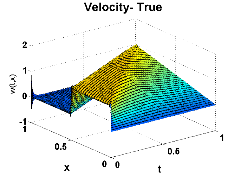
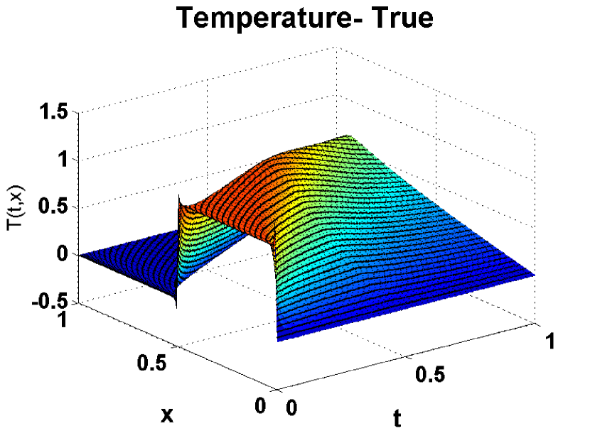
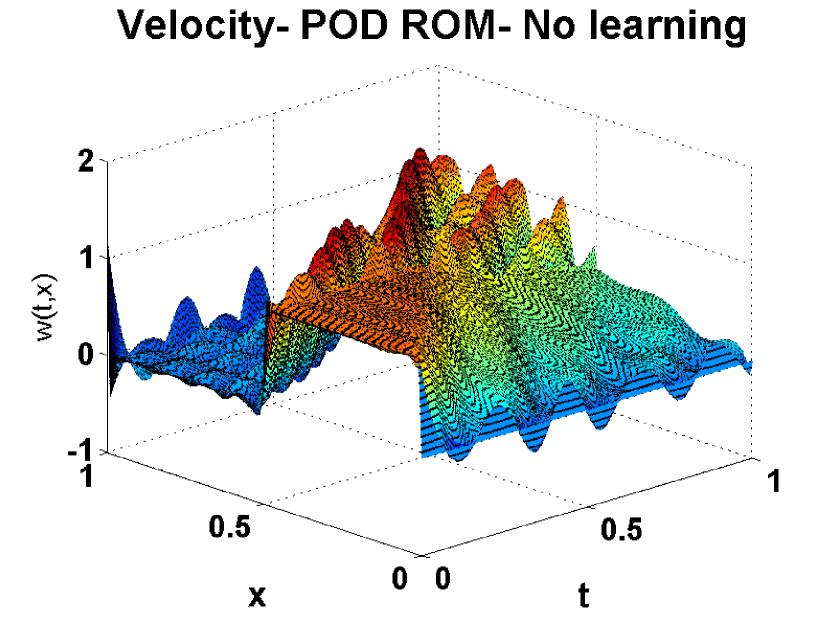
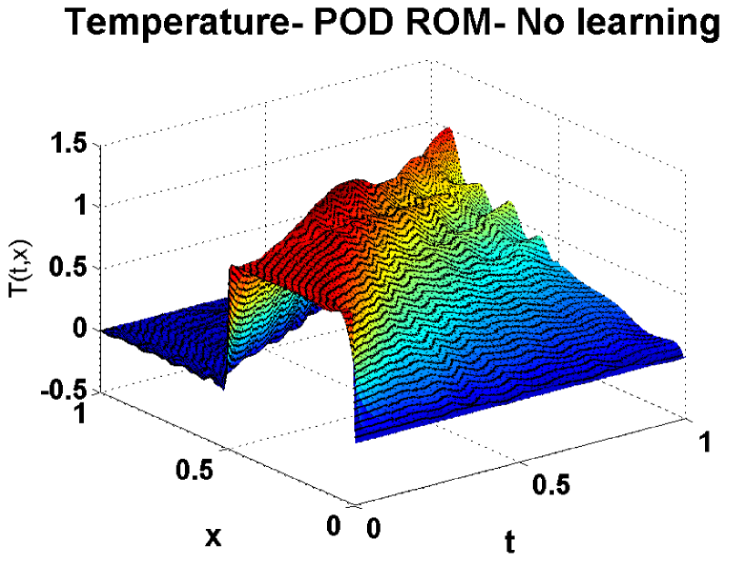
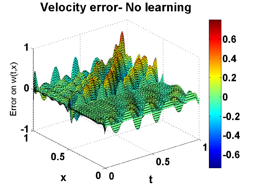
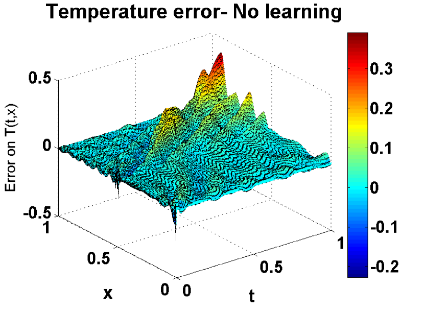
We first show for comparison purposes the true solutions, the high fidelity (‘truth’) solutions obtained via the FEM. Equation (32) is discretized in space with piecewise linear basis functions with 100 elements, and subsequently solved with ode45 in Matlab®. The true solutions are reported in Figure 1. We then report in figure 2, the solutions of the POD ROM-G (without learning). We can see clearly in these figures that the POD ROM-G solutions are not as smooth as the true solutions, particularly the velocity profile is very irregular, and the goal of the closure model tuning is to smoothen both profiles, as much as the closure model allows. For a clearer evaluation, we also report the errors between the true solutions and the POD ROM-G solutions, in Figure 3. 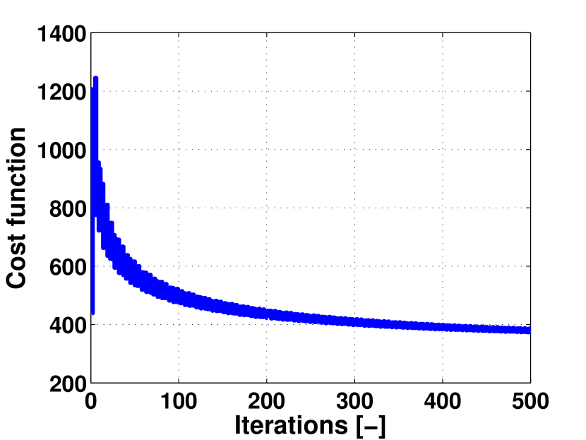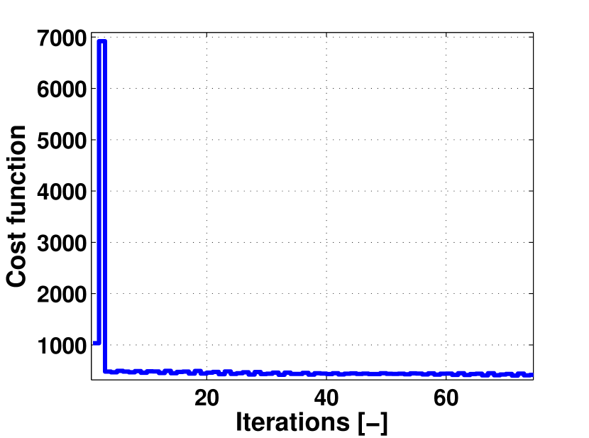Next, we apply the ES-based closure model auto-tuning algorithm of Lemma 1, and report the associated cost function in Figure 4(a). 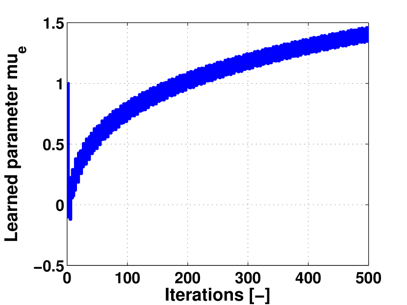We can clearly see a decrease of the learning cost function over the iterations, which means an improvement of the ROM prediction performance. The corresponding profile of the linear closure model amplitude over learning iterations is displayed in Figure 4(b), which shows that it reaches an optimal value around $\hat{\mu}_{e}\simeq 1.4$. As learning iterations proceed beyond the first $500$ displayed here, the values remain stable around the same points. 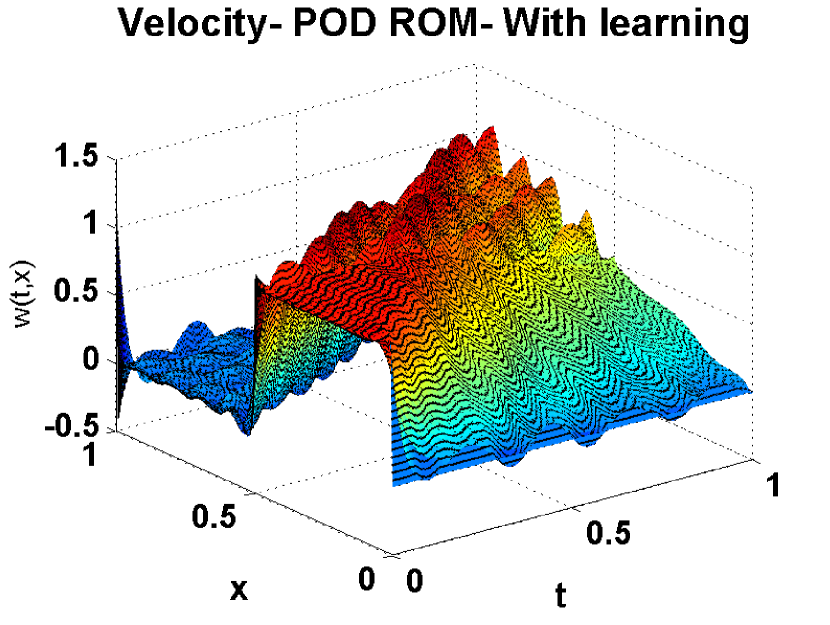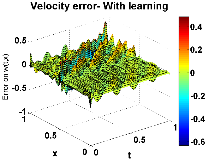Thus, for clarity of presentation, only a zoom around the first $500$ iterations is displayed. Finally, the corresponding ROM solutions are shown in Figure 5. For clearer evaluation of the optimal closure model stabilizing effect on the ROM, we also display in Figure 6 the errors between the exact PDE solutions and the stabilized ROM solutions.

IV-A2 Test 2

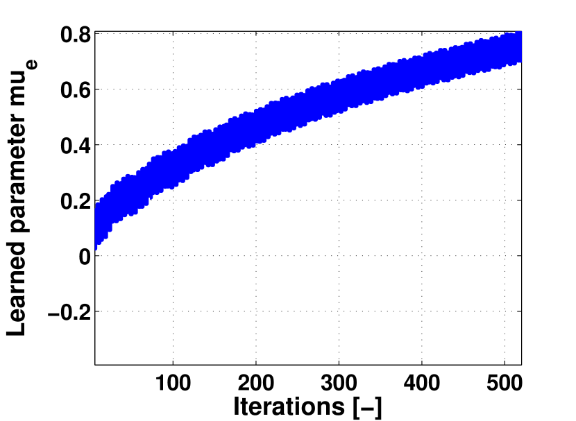
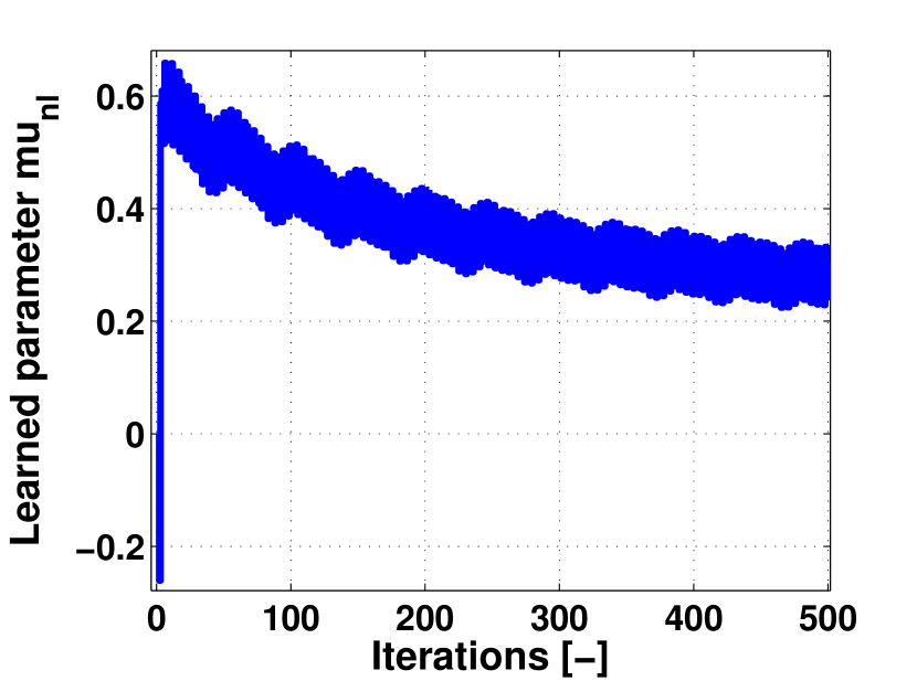
We report here the case related to Lemma 2, where we test the auto-tuning results of ES on the combination of a linear constant viscosity closure model and a nonlinear closure model. We apply Lemma 2, with the Heisenberg linear closure model given by (13). The two closure model amplitudes $\mu_{e}$ and $\mu_{nl}$ are tuned using the discrete version of the ES algorithm (29), given by

$$\begin{array}[]{l}y_{1}(k+1)=y_{1}(k)+a_{1}\;t_{f}\;\sin(\omega_{1}t_{f}k+\frac{\pi}{2})Q(\hat{\mu}_{e},{\hat{\mu}}_{nl}),\\ \hat{\mu}_{e}(k+1)=y_{1}(k+1)+a_{1}\;\sin(\omega_{1}t_{f}k-\frac{\pi}{2}),\\ y_{2}(k+1)=y_{2}(k)+a_{2}\;t_{f}\;\sin(\omega_{2}y_{2}(k+1)+\frac{\pi}{2})Q(\hat{\mu}_{e},{\hat{\mu}}_{nl}),\\ \hat{\mu}_{nl}(k+1)=y_{2}(k+1)+a_{2}\;\sin(\omega_{2}t_{f}k-\frac{\pi}{2}),\end{array}$$ (40)

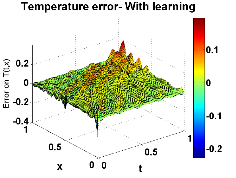
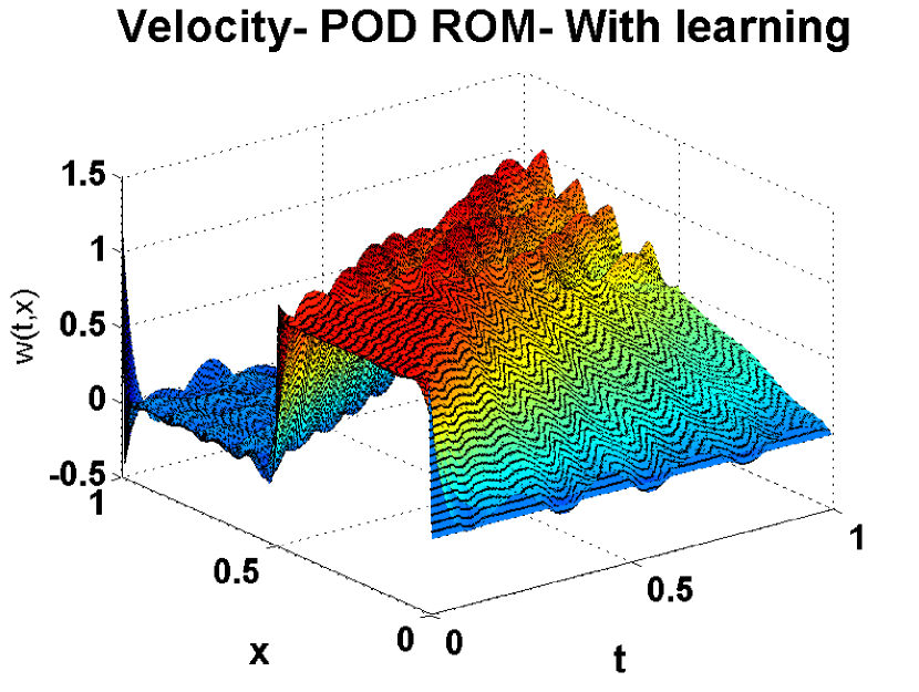
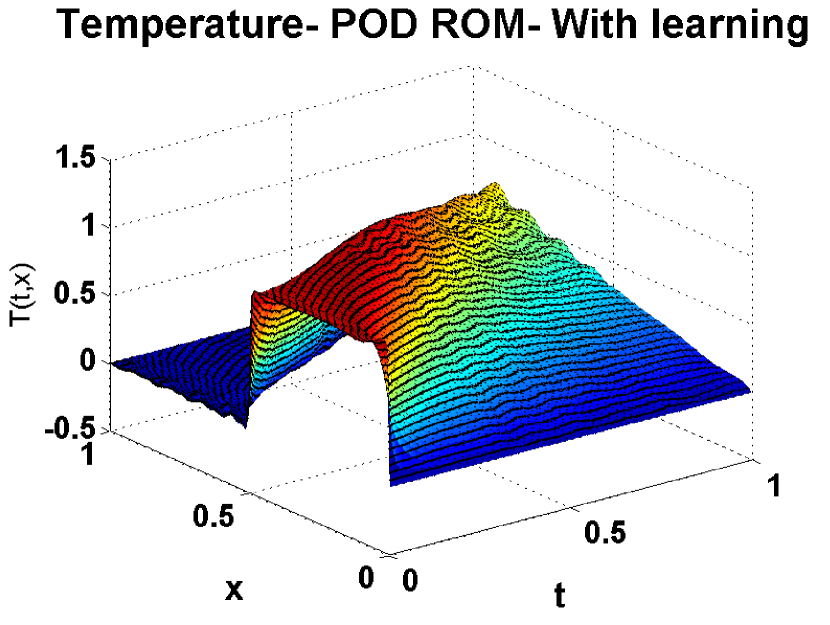
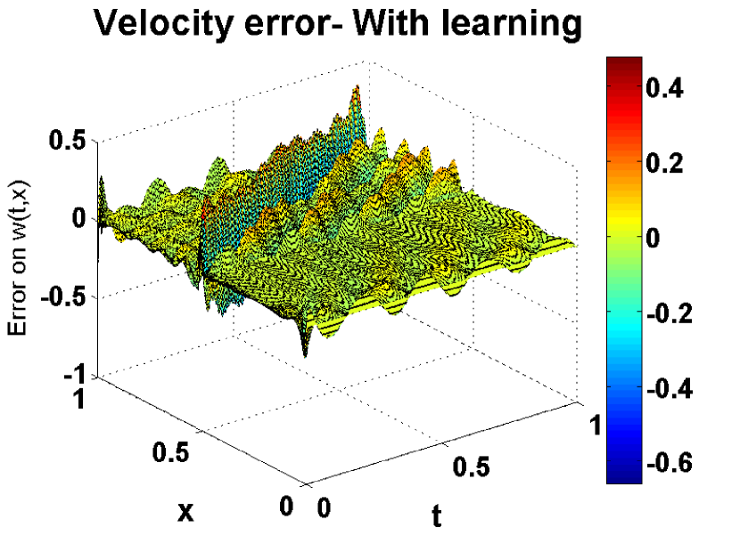
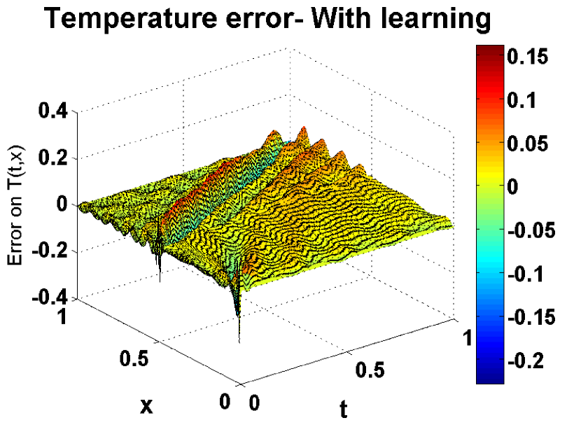
where $y_{1}(0)=y_{2}(0)=0$, and $k=0,1,2,...$ is the number of the learning iterations. We use the parameters’ values: $a_{1}=6\times 10^{-6}\;[-],\;\omega_{1}=10\;[\frac{rad}{sec}],\;a_{2}=6\times 10^{-6}\;[-],\;\omega_{2}=15\;[\frac{rad}{sec}]$, and a similar cost function as in Test 1. We show the profile of the learning cost function over the learning iterations in Figure 7(a). We can see a quick decrease of the cost function within the first $20$ iterations. This means that the ES manages to improve the overall solutions of the POD ROM very fast. The associated profiles for the two closure models’ amplitudes learned values $\hat{\mu}_{e}$ and $\hat{\mu}_{nl}$ are reported in figures 7(b), and 7(c). We can see that even though the cost function value drops quickly, the ES algorithm continues to fine-tune the values of the parameters $\hat{\mu}_{e}$, $\hat{\mu}_{nl}$ over the iterations, and they reach eventually reach an optimal values of $\hat{\mu}_{e}\simeq 0.3$, and $\hat{\mu}_{nl}\simeq 0.76$. We also show the effect of the learning on the POD ROM solutions in Figure 8, and figure 9, which by comparison with figures 2, and 3, show a clear improvement of the POD ROM solutions with the ES tuning of the closure models’ amplitudes. We also notice an improvement of the ROM solutions compared to the linear closure model stabilization test results of figure 6. Specifically, we see that the temperature error in the case of the closure model of Lemma 2, is smaller than the one obtained with the linear closure model of Lemma 1. We do not currently have a formal proof. However, we believe that the improvement is due to the fact that in the closure model of Lemma 2, we are using both the stabilizing effect of the linear viscosity closure model term and the stabilizing effect of the nonlinear closure model term.

(a) True velocity profile

(b) True temperature profile

Figure 1: True solutions of (32)

(a) Learning-free POD ROM velocity profile

(b) Learning-free POD ROM temperature profile

Figure 2: Learning-free POD ROM solutions of (32)- No learning

(a) Error between the true velocity and the learning-free POD ROM velocity profile

(b) Error between the true temperature and the learning-free POD ROM temperature profile

Figure 3: Errors between the nominal POD ROM and the true solutions- No learning

(a) Learning cost function vs. number of iterations

(b) Learned parameter $\hat{\nu_{e}}$ vs. number of iterations

Figure 4: Learned parameters and learning cost function- Stabilization with learning- Linear closure model

(a) Learning-based POD ROM velocity profile

(b) Learning-based POD ROM temperature profile

Figure 5: Learning-based POD ROM solutions of (32)- Stabilization with learning- Linear closure model

(a) Error between the true velocity and the learning-based POD ROM velocity profile

(b) Error between the true temperature and the learning-based POD ROM temperature profile

Figure 6: Errors between the learning-based POD ROM and the true solutions- Stabilization with learning- Linear closure model

(a) Learning cost function vs. number of iterations

(b) Learned parameter $\hat{\nu_{e}}$ vs. number of iterations

(c) Learned parameter $\hat{\nu_{nl}}$ vs. number of iterations

Figure 7: Learned parameters and learning cost function- Stabilization with learning- Nonlinear closure model

(a) Learning-based POD ROM velocity profile

(b) Learning-based POD ROM temperature profile

Figure 8: Learning-based POD ROM solutions of (32)- Stabilization with learning- Nonlinear closure model

(a) Error between the true velocity and the learning-based POD ROM velocity profile

(b) Error between the true temperature and the learning-based POD ROM temperature profile

Figure 9: Errors between the learning-based POD ROM and the true solutions- Stabilization with learning- Nonlinear closure model

V Conclusion and discussion

In this work, we explore the problem of stabilization of reduced order models for partial differential equations, focusing on the closure model-based ROM stabilization approach. It is well known that tuning the closure models’ gains is an important part in obtaining good stabilizing performances. Thus, we propose a learning ES-based auto-tuning method to optimally tune the gains of linear and nonlinear closure models, and achieve an optimal stabilization of the ROM. We validate our using the coupled Burgers’ equation as an example, demonstrating significant gains in error performance. The results are encouraging. We defer to future publications verifying our approach on more challenging higher dimensional cases. Our results also raise the prospect of developing new nonlinear closure models, together with their auto-tuning algorithms using extremum seeking, as well as other machine learning techniques.

References

- [1] L. Cordier, B. Noack, G. Tissot, G. Lehnasch, J. Delville, M. Balajewicz, G. Daviller, and R. K. Niven, “Identification strategies for model-based control,” Experiments in Fluids, vol. 54, no. 1580, pp. 1–21, 2013.
- [2] M. Balajewicz, E. Dowell, and B. Noack, “Low-dimensional modelling of high-reynolds-number shear flows incorporating constraints from the Navier Stokes equation,” Journal of Fluid Mechanics, vol. 729, no. 1, pp. 285–308, 2013.
- [3] M. Balajewicz, “Lyapunov stable galerkin models of post-transient incompressible flows,” arXiv.org/physics /arXiv:1312.0284, Tech. Rep., December 2013.
- [4] O. San and J. Borggaard, “Basis selection and closure for POD models of convection dominated Boussinesq flows,” in 21st International Symposium on Mathematical Theory of Networks and Systems, Groningen- The Netherlands, July 2014, pp. 132–139.
- [5] O. San and T. Iliescu, “Proper orthogonal decomposition closure models for fluid flows: Burgers equation,” International Journal of Numerical Analyis and Modeling, vol. 1, no. 1, pp. 1–18, 2013.
- [6] W. Haddad and V. S. Chellaboina, Nonlinear dynamical systems and control: a Lyapunov-based approach. Princeton University Press, 2008.
- [7] P. Holmes, J. L. Lumley, and G. Berkooz, Turbulence, coherent structures, dynamical systems and symmetry. Cambridge university press, 1998.
- [8] O. Sordalen, “Optimal thrust allocation for marine vessels,” Control Engineering Practice, vol. 15, no. 4, pp. 1223–1231, 1997.
- [9] C. A. J. Fletcher, “The group finite element formulation,” Computer Methods in Applied Mechanics and Engineering, vol. 37, pp. 225–244, 1983.
- [10] K. Kunisch and S. Volkwein, “Galerkin proper orthogonal decomposition methods for a general equation in fluid dynamics,” SIAM Journal on Numerical Analysis, vol. 40, no. 2, pp. 492–515, 2007.
- [11] B. Kramer, P. Grover, P. Boufounos, M. Benosman, and S. Nabi, “Sparse sensing and dmd based identification of flow regimes and bifurcations in complex flows,” arXiv, 2015.
- [12] K. Veroy and A. Patera, “Certified real-time solution of the parametrized steady incompressible navier-stokes equations: rigorous reduced-basis a posteriori error bounds,” International Journal for Numerical Methods in Fluids, vol. 47, no. 8, pp. 773–788, 2005.
- [13] Z. Wang, I. Akhtar, J. Borggaard, and T. Iliescu, “Proper orthogonal decomposition closure models for turbulent flows: A numerical comparison,” Computer Methods in Applied Mechanics and Engineering, vol. 237-240, pp. 10–26, 2012.
- [14] D. Rempfer, “Koharente strukturen und chaos beim laminar-turbulenten grenzschichtumschlag,” PhD, University of Stuttgart, 1991.
- [15] E. Tadmor, “Convergence of spectral methods for nonlinear conservation laws,” SIAM Journal on Numerical Analysis, vol. 26, no. 1, pp. 30–44, 1989.
- [16] S. Sirisup and G. E. Karniadakis, “A spectral viscosity method for correcting the long-term behavior of pod models,” Journal of compuatational Physics, vol. 194, no. 1, pp. 92–116, 2004.
- [17] J. P. Chollet, Two-point closure used for a sub-grid scale model in large eddy simulations. In: Turbulent Shear Flows 4. Springer, 1984, ch. Two-point closure used for a sub-grid scale model in large eddy simulations, pp. 62–72.
- [18] M. Lesieur and O. Metais, “New trends in large-eddy simulations of turbulence,” Annual Review of Fluid Mechanics, vol. 28, no. 1, pp. 45–82, 1996.
- [19] G. S. Karamanos and G. E. Karniadakis, “A spectral vanishing viscosity method for large-eddy simulations,” Journal of Computational Physics, vol. 163, no. 1, pp. 22–50, 2000.
- [20] M. Rotea, “Analysis of multivariable extremum seeking algorithms,” in Proceedings of the American Control Conference, vol. 1, no. 6, Sep 2000, pp. 433–437.
- [21] B. Noack, M. Schlegel, B. Ahlborn, G. Mutschke, M. Morzynski, P. Comte, and G. Tadmor, “A finite-time thermodynamics of unsteady fuid fows,” Journal of Non-Equilibrium Thermodynamics, vol. 33, no. 2, pp. 103–148, 2008.
- [22] B. R. Noack, M. Morzynski, and G. Tadmor, Reduced-Order Modelling for Flow Control, 1st ed., ser. 528. Springer-Verlag Wien, 2011.
- [23] B. Kramer, “Model reduction of the coupled burgers equation in conservation form,” Masters of Science in Mathematics, Virginia Polytechnic Institute and State University, 2011.