Spin Flips – II. Evolution of dark matter halo spin orientation, and its correlation with major mergers

Abstract

We expand our previous study on the relationship between changes in the orientation of the angular momentum vector of dark matter haloes (“spin flips”) and changes in their mass (Bett & Frenk, 2012), to cover the full range of halo masses in a simulation cube of length $100\,h^{-1}\mathrm{Mpc}$. Since strong disturbances to a halo (such as might be indicated by a large change in the spin direction) are likely also to disturb the galaxy evolving within, spin flips could be a mechanism for galaxy morphological transformation without involving major mergers. We find that $35\%$ of haloes have, at some point in their lifetimes, had a spin flip of at least $45\degr$ that does not coincide with a major merger. Over $75\%$ of large spin flips coincide with non-major mergers; only a quarter coincide with major mergers. We find a similar picture for changes to the inner-halo spin orientation, although here there is an increased likelihood of a flip occurring. Changes in halo angular momentum orientation, and other such measures of halo perturbation, are therefore very important quantities to consider, in addition to halo mergers, when modelling the formation and evolution of galaxies and confronting such models with observations.

1 Introduction

One of the key quantities in the evolution of cosmic strucures and the formation of galaxies is angular momentum. The acquisition and early growth of angular momentum by dynamically relaxed, overdense clumps of matter (‘haloes’) can be studied using linear tidal torque theory (Hoyle 1951; Peebles 1969; Doroshkevich 1970a, b; White 1984; Catelan & Theuns 1996a, b; see also Porciani et al. 2002, Schäfer 2009 and Codis et al. 2015), but this begins to break down as structure growth becomes non-linear (White, 1984). Subsequent growth then has to be studied using $N$-body simulations. While research in this field dates back many decades, the continual increase in computing power means that recent simulations have been able to determine with great accuracy the distribution and evolution of the halo angular momentum amplitudes (e.g. Bullock et al. 2001; Avila-Reese et al. 2005; Shaw et al. 2006; Hahn et al. 2007b, a; Bett et al. 2007, 2010; Macciò et al. 2007, 2008; Knebe & Power 2008; Muñoz-Cuartas et al. 2011).

In contrast, the orientation of halo angular momentum is less well studied. Research on this topic tends to focus on the angular momentum direction with respect to other quantities, such as the shape of the halo (e.g. Warren et al., 1992; Bailin & Steinmetz, 2005; Allgood et al., 2006; Shaw et al., 2006; Hayashi et al., 2007; Bett et al., 2007, 2010), or the orientation of galaxies (e.g. van den Bosch et al., 2002; van den Bosch et al., 2003; Chen et al., 2003; Gustafsson et al., 2006; Croft et al., 2009; Romano-Díaz et al., 2009; Bett et al., 2010; Agustsson & Brainerd, 2010; Hahn et al., 2010; Deason et al., 2011), or larger-scale filaments and voids (e.g. Bailin & Steinmetz, 2005; Hahn et al., 2007b, a; Brunino et al., 2007; Paz et al., 2008; Cuesta et al., 2008; Hahn et al., 2010; Libeskind et al., 2012). In particular, Codis et al. (2012) found that low-mass haloes, which have grown through smooth accretion, tend to have their spin vectors aligned parallel to their nearest filament. In contrast, spins in higher mass haloes, which have experienced major mergers, tend to be perpendicular to their filaments. Dubois et al. (2014) showed that this is also true for galaxies. Experiencing more mergers increases the likelihood of perpendicular alignment, whereas a lack of mergers allows a galaxy spin to drift back towards parallel alignment with its filament (Welker et al., 2014).

The evolution of the Lagrangian mass comprising $z=0$ haloes has been studied by Sugerman et al. (2000) and Porciani et al. (2002), who showed that the spin direction changes due to non-linear evolution, with both the average deviation from the initial direction, and the scatter in that angle, increasing with time.

Part of the reason for the importance of angular momentum is the strong link it provides between halo and galaxy evolution. In the standard cosmological model, the matter content of the Universe is dominated by a cold, collisionless component, cold dark matter (CDM). In this paradigm, structures grow hierarchically, through mergers of ever-larger objects. Galaxies then form and evolve within these haloes (White & Rees, 1978; White & Frenk, 1991). The more complex physical processes available to the baryons as they cycle between gas and stars result in galaxy evolution not being strictly hierarchical (e.g. Bower et al., 2006). In models of galaxy formation, the gas is usually assumed to have initially the same angular momentum as the halo, which is then conserved as the gas cools and collapses to form a disc. Thus, the size of the galactic disc is directly related to the dark matter halo’s angular momentum (Fall & Efstathiou, 1980; Mo et al., 1998; Zavala et al., 2008). This idea is widely implemented in semi-analytic models of galaxy formation (White & Frenk 1991; see also the reviews of Baugh 2006 and Benson 2010). It is important to note that this involves only the magnitude of the halo angular momentum, rather than the full vector quantity. It is the vector that is conserved, and standard semi-analytic models at present make no reference to the angular momentum direction.

Morphological changes in galaxies can be brought about through tidal forces (Toomre & Toomre, 1972), and indeed a galactic disc can be disrupted completely if the gravitational potential varies strongly enough over a short timescale. Galaxy formation models thus assume that a sufficiently large galaxy merger event will destroy a disc, randomising the stellar orbits and forming a spheroid (e.g. Toomre, 1977; Barnes, 1988, 1992; Barnes & Hernquist, 1996; Hernquist, 1992, 1993). This has been shown also to occur in numerical simulations of individual mergers (e.g. Naab & Burkert, 2003; Bournaud et al., 2005; Cox et al., 2006; Cox et al., 2008). However, the details of the merger process, and the properties of the resulting galaxies, depend strongly on the gas richness of the participants (e.g. Stewart et al., 2008, 2009; Hopkins et al., 2009b; Hopkins et al., 2009a, 2010; Moster et al., 2010), and on the details of the star formation and feedback processes triggered by the merger (e.g. Okamoto et al., 2005; Zavala et al., 2008; Scannapieco et al., 2009).

In Bett & Frenk (2012) (hereafter Paper I), the authors put forward the idea that sudden, large changes in the direction of the halo angular momentum vector (hereafter halo spin direction, for brevity) are indicative of a significant disturbance to the halo, and that, although such changes are usually assumed to only accompany halo mergers, they can also occur without the large mass gain implied by a merger. This would mean that galaxies could be distrupted by processes that are not captured in the galaxy and halo merger trees used in most current modelling, and that sudden changes to the halo angular momentum direction could be a useful proxy to detect such events.

Such events have been seen in $N$-body and hydrodynamical simulations. Okamoto et al. (2005) found that their simulated disc galaxy flipped its orientation (Bett, 2010), with subsequent misaligned gas accretion resulting in a transformation into a bulge, with another disc forming later. Scannapieco et al. (2009) also found that misalignment of a stellar disc with accreting cold gas can result in bulge formation, sometimes destroying the disc, and sometimes with a new disc forming later. The idealized experiments of Aumer & White (2013) showed clearly the strong and complex impact of gas/halo misalignment on the evolution of the disc and bulge components of a halo’s central galaxy. Romano-Díaz et al. (2009) analysed haloes in simulations both with and without baryons, and found that halo spin orientations can change much more drastically than the angular momentum magnitude, and that such large orientation changes are not restricted to major mergers. Welker et al. (2015) also found that it is not just major mergers that can destroy disks, although minor mergers are statistically less likely to do so; the gas content in the galaxies also has an important role.

Following these studies, Padilla et al. (2014) used the distribution of spin flips from haloes in the Millennium II simulation (Boylan-Kolchin et al., 2009) to incorporate their impact stochastically in a semi-analytic galaxy formation model. In their model, flips in galaxy discs act to reduce the disc spin in proportion to the cosine of the orientation change, i.e. larger flips reduce the spin of the disc more. Their model also allows disc instabilities, which cause bursts of star formation, to be triggered by spin flips, rather than by halo mergers explicitly. The authors demonstrate the positive impact that these changes to the model have on the distributions of galaxy properties at different redshifts, such as galaxy luminosity functions, morphological distributions and star formation rates.

In the present paper, we study the relationship between changes in spin orientation and halo merger history, expanding on Paper I. We include haloes of all masses in the $N$-body simulation we use, and pay special attention to those haloes that do not survive to $z=0$; we also compare our results against the assumptions of mass and angular momentum conservation used in simple halo models. The results emphasize the need for models of galaxy formation to include more information than just the halo mass accretion history when determining galaxy properties, and in particular the transfer of material from disc to spheroidal structures.

In Section 2 we describe the simulation used, the identification and selection of haloes and their merger trees, and the properties on which we focus in our analysis. Section 3 describes our results, both in terms of the distribution of events over all haloes, and during each halo’s lifetime, including the impact on inner halo spin directions. We summarise our conclusions in Section 4.

2 Simulation data and analysis

We use the same simulation and methods for analysis as in Paper I. While we describe the important points here, we refer the reader to that paper for further details.

2.1 The hMS simulation, haloes and merger trees

We use a cosmological dark matter $N$-body simulation that has been referred to as hMS, since it was made using the same L-Gadget-2 code and $\Lambda$CDM cosmological parameters as the Millennium Simulation (MS, Springel et al., 2005), but with a smaller cube size ($100\,h^{-1}\mathrm{Mpc}$) and higher resolution ($900^{3}$ particles of mass $9.518\times 10^{7}\,h^{-1}\mathrm{M}_{\sun}$, and softening $2.4\,h^{-1}\mathrm{kpc}$). The hMS assumes the same cosmological parameters as the MS: writing cosmological density parameters as $\Omega_{i}(z)=\rho_{i}(z)/\rho_{\mathrm{crit}}(z)$, in terms of the mass density of component $i$ and the critical density $\rho_{\mathrm{crit}}(z)=3H(z)^{2}/(8\pi G)$, where the Hubble parameter is $H(z)$, for the present-day cosmological constant, total mass, and baryonic mass, the hMS uses values of $\Omega_{\Lambda 0}\equiv\Omega_{\Lambda}(z=0)=0.75$, $\Omega_{\mathrm{M}0}=0.25$, and $\Omega_{\mathrm{b}0}=0.045$ respectively. The present-day value of the Hubble parameter is parameterised in the standard way as $H_{0}=100h\,\mathrm{km}\,\mathrm{s}^{-1}\,\mathrm{Mpc}^{-1}$, where $h=0.73$. The spectral index is $n=1.0$ and the linear-theory mass variance in $8\,h^{-1}\mathrm{Mpc}$ spheres at $z=0$ is given by $\sigma_{8}=0.9$.

We use a halo definition based on linking and separating subhaloes from their associated friends-of-friends (FoF) particle groups according to information in the halo merger trees. The algorithms for both the haloes and merger trees were originally described in Harker et al. (2006), and designed for use with the implementation of the Galform semi-analytic galaxy formation model in the Millennium Simulation (Bower et al., 2006). Particle groups are first identified through the Friends of Friends (FoF) algorithm (Davis et al., 1985), with a linking length parameter of $b=0.2$. Self-bound substructures – the main bulk of the halo itself, plus any subhaloes – are then identified using the Subfind code (Springel et al., 2001). Each halo-candidate particle group then consists of a main self-bound structure, zero or more self-bound subhaloes, plus additional particles that are spatially linked through FoF.

The bound subtructures can be tracked between the simulation snapshots, identifying progenitors and descendents (see e.g. Paper I, Harker et al. 2006 or Jiang et al. 2014 for details). Using this additional evolution information the halo catalogue is refined, by separating off subhaloes that are spatially but not dynamically linked to the halo. For example, subhaloes that are just passing through the outskirts of a larger halo are separated. Two haloes joined by a thin bridge of particles (as commonly occurs with FoF) would also be split apart. Bett et al. (2007) compared the spins, shapes, clustering and visual appearance of these ‘merger-tree haloes’ against both simple FoF groups and haloes defined using a simple spherical overdensity criterion, and showed that this merger-tree method offers a great improvement in terms of identifying the genuine physical structure of a halo.

The result of the merger tree and halo identification algorithms is a set of haloes (groups of self-bound structures) identified at each snapshot, with at most one descendent and zero or more progenitors. Each halo identified at $z=0$ is the root of its own tree, which branches into many progenitor haloes at earlier timesteps. In this paper, we wish to study how properties of individual haloes evolve. We therefore identify the evolutionary “track” of a halo, by finding the most massive of its immediate progenitors at each timestep. We give an illustration of halo tracks in a merger tree in Fig. 1. The track of the root halo is marked in red: each red halo is the most massive progenitor of its descendent halo. The halo population at a given snapshot is made up of many other haloes than the root halo however: tracks of other haloes exist, which do not survive until $z=0$. Instead, they merge into a more massive halo at some point. The endpoint of each track in Fig. 1 is highlighted in heavy black lines. Also note that some tracks have no evolution information, since they only exist at one timestep before merging into a larger halo.

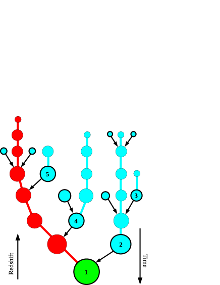
Figure 1: Schematic of a single merger tree. Each circle represents a halo, with each row representing a single simulation output time. The green “root” halo is that identified at $z=0$. The evolutionary track of the most-massive progenitors of the root halo is coloured in red. Tracks of haloes that merge into a larger halo before $z=0$ are coloured cyan. End-points of tracks have a heavy black outline, with their final merger into a larger neighbour marked with a black arrow. Six of these 11 tracks only exist at a single timestep, leaving five (marked with numbers) with useful halo-evolution data.

It is important to note that neither the halo definition nor the merger tree algorithm are by any means unique. The halo merger trees used in the semi-analytic galaxy formation models of Springel et al. (2005) and De Lucia & Blaizot (2007), which also use the Millennium Simulation, construct both the haloes and merger trees differently, although based on similar principles. Other methods that use splitting/stitching algorithms similar to the one used here include those by Wechsler et al. (2002), Fakhouri & Ma (2008, 2009), Genel et al. (2009), Neistein et al. (2010); see also Maller et al. (2006). There have recently been various detailed comparison studies of halo definition and merger tree algorithms, including Tweed et al. (2009); Knebe et al. (2013); Srisawat et al. (2013); Avila et al. (2014). There is therefore significant scope for similar studies to ours to produce quantitatively different results.

2.2 Halo property catalogues

As in Paper I, various properties of the haloes are computed at each snapshot in time, in the centre-of-momentum frame of each halo, and in physical rather than comoving coordinates. The halo centre is identified with the location of the gravitational potential minimum of its most massive structure, as found by Subfind. Properties are computed using the halo particles only (rather than the set of particles within a certain radius), and include the halo mass $M$, kinetic and potential energies $T$ and $U$, and angular momentum vector J. An approximate “virial” radius $R_{\mathrm{vir}}$, is found by growing a sphere around the halo centre until the enclosed density from halo particles drops below $\Delta_{\mathrm{c}}(z)\,\rho_{\mathrm{crit}}(z)$. The threshold overdensity with respect to critical, $\Delta_{\mathrm{c}}(z)$, is given by the spherical collapse model (Eke et al., 1996), using the fitting formula of Bryan & Norman (1998):

$$\Delta_{\mathrm{c}}(z)=18\pi^{2}+82\left(\Omega_{\mathrm{M}}(z)-1\right)-39\left(\Omega_{\mathrm{M}}(z)-1\right)^{2}$$ (1)

In the case of the flat $\Lambda$CDM universe here, we can write $\Omega_{\mathrm{M}}(z)=\Omega_{\mathrm{M}0}a^{-3}/\chi(z)$ and $\rho_{\mathrm{crit}}(z)=\rho_{\mathrm{crit,}0}\,\chi(z)$, where the expansion factor $a=(1+z)^{-1}$ and we define $\chi(z)=\Omega_{\mathrm{M}0}a^{-3}+\Omega_{\Lambda 0}$ for convenience. Note that we only use $R_{\mathrm{vir}}$ as a convenient spatial scale for the haloes, rather than as a halo boundary. We also define an inner-halo region at $r_{\mathrm{inner}}=0.25R_{\mathrm{vir}}$ ( following the orientation resolution tests of Bett et al. 2010). Using the mass within this radius, we also compute the inner angular momentum vector $\textbf{{J}}_{\mathrm{inner}}$.

2.3 Halo selection

We need to select haloes at each timestep from which reliable measurements of angular momentum can be made. We follow the Three Rs of selecting haloes from simulations, requiring them to be well-resolved, approximately relaxed, and robust against effects caused by using discrete particles. These are realised through the following selection criteria, respectively:

$$N_{\mathrm{p}} \geq N_{\mathrm{p,lim}}$$

$$\left|Q\right| \leq Q_{\mathrm{lim}},$$

$$\log_{10}\tilde{\jmath} \geq \log_{10}\tilde{\jmath}_{\mathrm{lim}},$$

where $N_{\mathrm{p}}$ is the number of particles comprising the halo, the energy ratio $Q=2T/U+1$ approximates the virial ratio, and $\tilde{\jmath}=j/\sqrt{GM_{\mathrm{h}}R_{\mathrm{vir}}}$ represents a scaling of the halo angular momentum magnitude with respect to that of a particle orbiting under gravity at the virial radius ($j=J/M$ is the specific angular momentum). Following resolution tests in the studies of Bett et al. (2007, 2010), we choose limiting values of $N_{\mathrm{p,lim}}=1000$ (that is, halo masses greater than $\sim 10^{11}\,h^{-1}\mathrm{M}_{\sun}$), $Q_{\mathrm{lim}}=0.5$, and $\log_{10}\tilde{\jmath}_{\mathrm{lim}}=-1.5$. When considering changes to the inner halo, the criteria for $N_{\mathrm{p}}$ and $\tilde{\jmath}$ are replaced by limits on $N_{\mathrm{p,inner}}$ and $\tilde{\jmath}_{\mathrm{inner}}$, using the same threshold values.

As in Paper I, we apply two additional selection criteria suggested by a visual inspection of the time series of properties of individual haloes. Firstly, we use a simple measure of “formation time”: we restrict our analysis to the time period after the last time when $M(z)<M_{\mathrm{form}}$, and choose $M_{\mathrm{form}}=0.5M_{0}$ (where $M_{0}$ is the halo mass at $z=0$). Before this time, haloes tend to have a much higher rate of accretion and mergers, and experience a general instability in their properties. Excluding this period ensures that this does not dominate our results. While this undoubtedly affects the number of major mergers that we expect to see in our sample, we are still interested in how spin orientation changes are distributed amongst mass changes large and small; we’re not explicitly excluding post-‘formation’ major mergers.

Secondly, we found that the halo finder and merger tree algorithms sometimes joined a satellite halo into a larger object as a subhalo, then separated it off again at the next timestep, perhaps merging again later. This will clearly cause large apparent changes to the halo angular momentum, mimicking a physical spin flip; however it is due to uncertainty in the halo boundary, rather than a physical change in the halo angular momentum. In order to eliminate such “fake flips”, we exclude events with large changes in the virial ratio; in particular, events with $\Delta Q\leq-0.3$ are excluded. Since this effect is due to uncertainties in the halo boundary, we do not apply this exclusion criterion when considering the inner halo spin.

Finally, we note that we analyse our halo population over the redshift range $z<6.2$; in any case, the effects we describe will be most observable at low redshift.

2.4 Evolution of halo properties

Combining the merger tree data with the halo catalogues at each timestep means we can obtain the time series of the evolution of each halo property, for each halo (more precisely: for each halo track, both those that survive until $z=0$ and those that do not). As in Paper I, we are most interested in the changes in halo mass and spin orientation over time. We therefore define the same two key quantities used in the previous paper, the fractional mass change,

$$\Delta\mu(t):=\frac{M(t)-M(t-\tau)}{M(t)},$$ (2)

and the change in spin orientation

$$\cos\theta(t):=\frac{\textbf{{J}}(t)\mathbf{\cdot}\textbf{{J}}(t-\tau)}{\left|\textbf{{J}}(t)\right|\left|\textbf{{J}}(t-\tau)\right|}$$ (3)

where $\tau$ is the timescale over which we measure the halo property change (the time $t-\tau$ precedes the time $t$).

To allow a fair comparison between spin flips in different sizes of haloes at different times, we use a constant timescale $\tau$, rather than simply using the (irregular) time difference between simulation snapshots. We linearly interpolate halo properties between snapshots to get their values at each ‘previous’ time $t-\tau$. (The simulation snapshots are sufficiently well spaced in time that a more complex interpolation scheme is unnecessary) We choose an event timescale of $\tau=0.5\,\mathrm{Gyr}$. The snapshot spacing and the impact of our choice of dynamic timescale are shown in Appendix A.

We will refer to the halo property changes at a given timestep, $\Delta\mu(t)$ and $\cos\theta(t)$, generically as an event. We shall use some fiducial values to divide the distribution of events and aid interpretation: We consider a spin direction change of at least $\theta_{0}=45\degr$ to be ‘large’, and a fractional mass change of more than $\Delta\mu_{0}=0.3$ to correspond to a major merger. For the sake of brevity, we shall often refer to events with $\Delta\mu\leq 0.3$ as minor mergers, even though they could be smooth accretion (i.e. mass gain from particles that were not from a separate satellite halo), or even mass loss. Note that the only restriction on $\Delta\mu$ is that it must be below unity. A value of $\Delta\mu=\frac{1}{3}$ corresponds to a mass gain of $50\%$; our fiducial value of $\Delta\mu=0.3$ results in a slightly smaller gain of $\frac{3}{7}\approx 43\%$. If $\Delta\mu>\frac{1}{2}$, then the halo has more than doubled in mass. We expect such events to be rare (but not impossible), due to how the merger trees are constructed: we are always comparing a halo with its most massive progenitor. On the other hand, it is also possible for mass to be lost between timesteps, although again our prejudice is for this to be rare. A value of $\Delta\mu=-1$ corresponds to a mass loss of $50\%$.

Finally, note that, as we are focusing on events that can disturb a halo, we are not distinguishing between mergers of two similar-mass haloes and the accretion of multiple small haloes onto a larger one: both cases could be registered as ‘major mergers’ if they occur rapidly enough, such as between two snapshots. Similarly, we do not consider the direction of halo accretion. On the other hand, rapid merging of haloes from opposite directions (e.g. along a filament) is likely to result in rather chaotic changes in spin direction – the infalling haloes would have to have extremely well balanced angular momenta for them to cancel sufficiently for the direction of the vector to remain unchanged, even if their magnitudes nearly cancelled (although the mass gain would still mean that it would be seen as a ‘disruptive’ event). The frequency of such events would have to be assessed in simulations with higher time resolution, and we note that our results can, in that sense, be seen as a lower limit: more spin flips might be seen in simulations with more timesteps.

3 Results

3.1 Flips of the whole halo

3.1.1 Distribution of flip and merger events

The joint distribution of spin direction changes and fractional mass changes, for all $524\,668$ selected events from halo tracks after $z=6.2$, is shown in Fig. 2 (note that the colour scheme is logarithmic). The distribution is very broad, with a strong peak for events with minimal change ($\cos\theta\approx 1$, $\Delta\mu\approx 0$): There are $318\,747$ events ($60.8\%$) just in the range $-0.05<\Delta\mu\leq 0.05$ & $\cos\theta\geq 0.95$. The tail down to larger spin orientation changes (lower $\cos\theta$) appears biased towards positive mass change, i.e. mergers. Note however that many events have $\Delta\mu<0$, i.e. mass loss between timesteps. Such events can occur for a number of reasons: just ‘noise’ related to the halo finder and other algorithms, with individual particles being included/excluded from the haloes from one snapshot to the next; and genuine loss from dynamical encounters. While about $23\%$ of events have $\Delta\mu\leq 0$, only $3.7\%$ ($19\,173$) have $\Delta\mu\leq-0.1$. Substantial mass loss is even more rare: just $340$ events have $\Delta\mu\leq-1$, which corresponds to a mass loss of $50\%$.

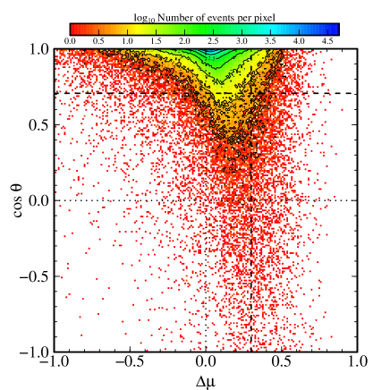
Figure 2: Event distribution in terms of fractional mass change, $\Delta\mu$, and angular momentum orientation change, $\cos\theta$. Dotted lines mark the origin, and dashed lines indicate our fiducial critical values for major mergers ($\Delta\mu>0.3$) and large flips ($\theta\geq 45\degr$). Contours are drawn at the levels given by the tickmarks on the colour bar.

To illustrate the shape of the distribution of selected events more quantitatively, we now look at cross-sections through it as histograms. Fig. 3 shows histograms of the spin orientation change for all halo tracks, plus for the subsections of the distribution that correspond to major mergers and minor mergers. The strong spike around “no change” is clearly visible, but the distribution is significantly broader if only major merger events are considered.

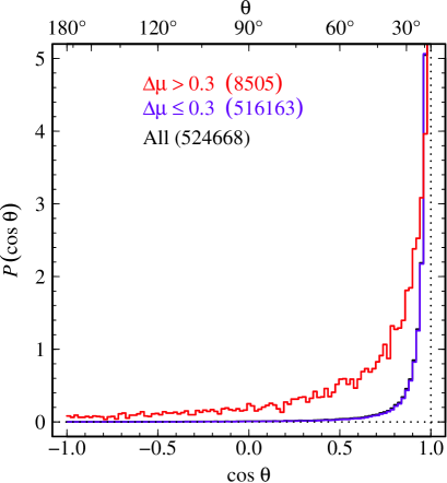
Figure 3: Histograms of $\cos\theta$, cross-sections of the event distribution shown in Fig. 2. The histogram of all events is plotted in black, with the subset corresponding to major mergers in red and minor mergers in blue. Note that the latter lies almost on top of the black line. The number of events selected in each case is written in the legend.

The histogram of halo fractional mass change, for all halo tracks plus the subsets of those that coincide with spin flips of two different magnitudes, is shown in Figure 4. Again, the spike at “no change” is clear, but the skewing of the peak of the distribution towards stronger mergers is also visible, particularly when the histogram is restricted to events with larger spin orientation changes.

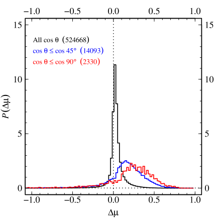
Figure 4: Histograms of $\Delta\mu$, cross-sections of the event distribution shown in Fig. 2. The histogram of all events is shown in black, while that of the subset of events with spin flips of at least $45\degr$ is shown in blue, and for spin flips of at least $90\degr$ is shown in red. The number of events selected in each case is written in the legend.

The cumulative distribution functions (CDFs) give us additional insight into the relationship between the distributions of spin flips and halo mass changes. We show the CDF of $\cos\theta$ in Fig. 5. This shows that minor mergers are very unlikely to coincide with a large flip: only $2\%$ of events without major mergers had flips of $45\degr$ or more. For the major merger events on the other hand, $39\%$ have spin flips of at least that magnitude. However, the CDF of $\Delta\mu$ (Fig. 6) shows that $76\%$ of large flips ($45\degr$ or more) coincide with minor mergers ($\Delta\mu\leq 0.3$). Although these results at first might seem contradictory, they are clearly evident in the shape of the distribution in Fig. 2, and stem from the very large number of minor merger events.

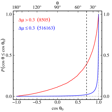
Figure 5: The cumulative distribution of events with spin orientation changes of at least $\theta_{0}$ degrees, from the distribution shown in Fig. 2. We show results of selecting just major merger events ($\Delta\mu>0.3$, red) and just minor merger events (blue). Our fiducial value of $\theta\geq 45\degr$ is marked with a dashed line.

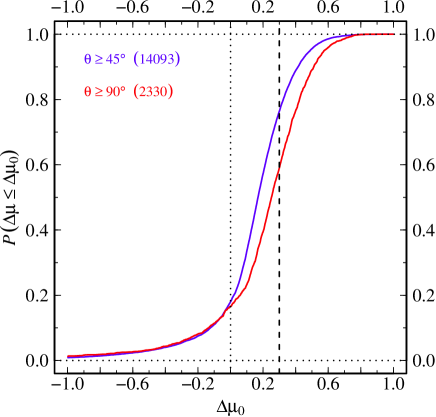
Figure 6: The cumulative distribution of events with fractional mass change of $\Delta\mu_{0}$ or less, from the distribution shown in Fig. 2. We show results of selecting just events with spin flips of at least $45\degr$ (blue) and at least $90\degr$ (red). Our fiducial value for major mergers, $\Delta\mu>0.3$, is marked with a dashed line.

We show in Fig. 7 the joint distribution of events in terms of the relative change in halo specific angular momentum magnitude versus the orientation change. This serves as an important reminder that a spin flip event does not necessarily mean that the spin magnitude has not also changed. Indeed, there is a weak tendency for large spin flips to correlate with an increase in the halo angular momentum. There are still a large number of flips in which the spin magnitude does not change, and the spin magnitude can change significantly without a corresponding orientation change.

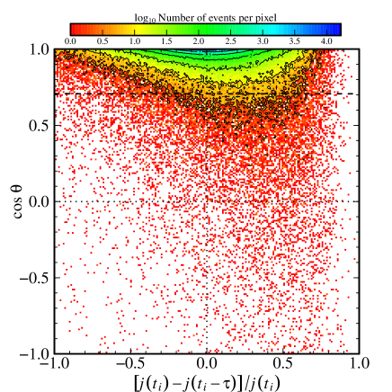
Figure 7: Event distribution analogous to Fig. 2, but in terms of the fractional specific angular momentum magnitude change instead of the fractional mass change ($j(t)=J(t)/M(t)$).

3.1.2 Root tracks vs. doomed tracks

We split the event distribution shown in Fig. 2 into that of events in the lives of the root haloes (those still extant at $z=0$) and events in the lives of ‘doomed’ haloes (those that merge into a more massive halo before $z=0$). The two resulting event distributions are shown in Fig. 8. Histograms for cross-sections through the root tracks’ distribution of $377\,484$ events are shown in Fig. 9. Although we can see the same basic trends here as in the previous figures (Figs. 2–4), the distributions are nonetheless noticeably different. The root tracks have a much narrower distribution in $\Delta\mu$, visible both at low and high values (mass loss and major mergers). Much of the broad tail to more negative $\Delta\mu$ seen in Fig. 2 for all tracks seems to come from the doomed tracks.

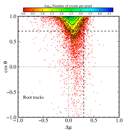
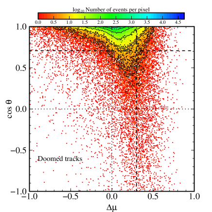
Figure 8: The distribution of events, as in Fig. 2, but split into just the $z=0$ root tracks only (top) and the doomed tracks only (bottom).

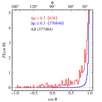
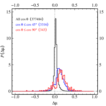
Figure 9: Histograms of the event distribution of root tracks (as shown in the top panel of Fig. 8), in terms of the spin orientation change (top) and the fractional mass change (bottom). These can be compared to Figs. 3 and 4.

The cumulative distributions of the events from the root tracks are shown in Fig. 10. When we consider just these haloes that survive to $z=0$, we find that less than $1\%$ of minor merger events have large spin flips, compared to $23.5\%$ of major mergers. However, over $95\%$ of spin flips of at least $45\degr$ coincide with minor mergers ($88\%$ for flips of at least $90\degr$).

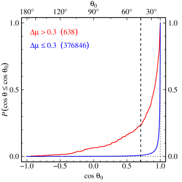
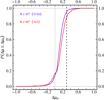
Figure 10: Cumulative distributions of events from haloes on root tracks (as shown in Fig. 8), as a function of flip threshold $\cos\theta_{0}$ (top) and merger threshold $\Delta\mu_{0}$ (bottom). These can be compared to Figs. 5 and 6.

3.2 The inner angular momentum

To have a noticeable effect on galaxy formation and evolution, it is reasonable to assume that it is the angular momentum in the inner regions of the halo in particular that needs to change. We have therefore also looked at the distribution of events from all halo tracks in terms of the angular momentum of the mass located within $0.25R_{\mathrm{vir}}$. We show the joint distribution of $\cos\theta_{\mathrm{inner}}$ and the total-halo mass change $\Delta\mu$ in the left panel of Fig. 11, with histogram cross-sections of the distribution (as before) in the centre and right panels. There is an increased likelihood of large spin flips of the inner halo relative to the total-halo results, although the tighter selection criteria (i.e. using $N_{\mathrm{p,inner}}$ and $\tilde{\jmath}_{\mathrm{inner}}$; see section 2.3) means there are fewer events slected overall ($150\,937$). This also results in far fewer mass-loss events being selected.

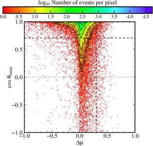
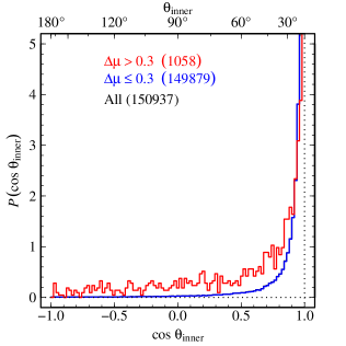
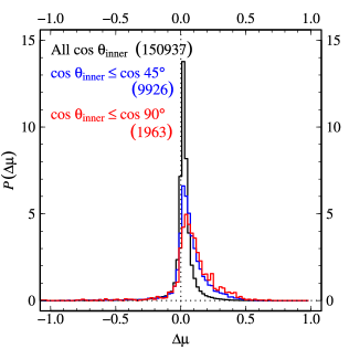
Figure 11: Left: Distribution of events from all halo tracks, in terms of the fractional mass change of the total halo, $\Delta\mu$, and the spin orientation change of the inner halo (i.e. the mass within $0.25R_{\mathrm{vir}}$). Centre: histogram cross-sections of the event distribution, through $\cos\theta_{\mathrm{inner}}$, for all selected events (black) and for the subsets that do (red) and do not (blue) coincide with major mergers. Right: histogram cross-sections through $\Delta\mu$, for all selected events (black) and for those with spin flips of at least $45\degr$ (blue) and $90\degr$ (red).

The cumulative distributions for the inner halo spin flip events are shown in Figs. 12 & 13. We find that minor merger events (the blue line in Fig. 12) are now much more likely to coincide with a large inner spin flip: about $6.3\%$, compared to $0.8\%$ for the total-halo flips shown in Fig. 5. The fraction of major merger events that also have significant inner flips is slightly increased, to $43\%$. When selecting just events with large inner flips (Fig. 13), we find a strong increase in the number that coincide with minor mergers: $95.4\%$ for flips of at least $45\degr$, and $91\%$ for flips of at least $90\degr$.

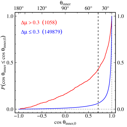
Figure 12: Cumulative distributions of events with inner spin misalignments of at least $\theta_{\mathrm{inner,}0}$ degrees. Events are selected as in Fig. 11. We show results taking the limiting total-halo fractional mass change to be $\Delta\mu_{0}=0.3$ (red: major mergers; blue: minor mergers/accretion).

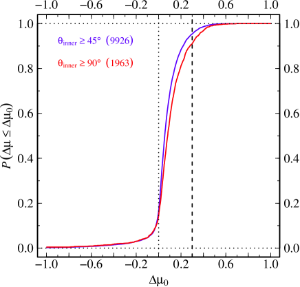
Figure 13: Cumulative distributions of events with fractional mass change of $\Delta\mu_{0}$ or less, from the event distribution shown in Fig. 11. We show results for selecting just events with inner spin flips of at least $45\degr$ (blue) and at least $90\degr$ (red).

We can also consider the distributions of $\cos\theta_{\mathrm{inner}}$ and $\Delta\mu$ for just the root tracks (Fig. 14). Just as for the total-halo spin, selecting only the root tracks results in a much narrower distribution of $\Delta\mu$. Although this does not change the cumulative distribution of minor-mergers much, there are far fewer large inner flips for the major-merger events (compare the middle panel with Fig. 12). The fraction of events with large inner flips that have minor mergers is even higher: over $99\%$ (of the $119\,450$ selected events) for flips of $45\degr$ of more.

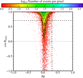
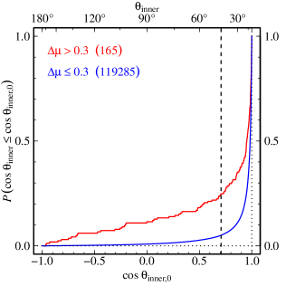
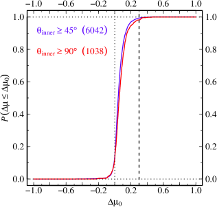
Figure 14: The joint distribution (left) and cumulative distributions (centre, right) of events from root haloes in terms of the total-halo mass change $\Delta\mu$ and inner-halo spin orientation change $\cos\theta_{\mathrm{inner}}$. These can be compared to Figs. 11, 12 & 13.

3.3 Coincidence of flips and mergers

It would be naïve to assume that, simply because the merger tree algorithm does not register a major merger occurring at exactly the same time as a spin flip, the spin flip is not physically associated with a major merger. For example, a major merger could have occurred at a slightly earlier or slightly later timestep in the simulation.

In fact, a visual inspection of the co-evolution of halo properties for individual objects suggests that many large spin flips that appear to coincide with minor mergers actually do have a major merger associated with them, albeit at an earlier or later time. For example, the orbit of a satellite halo might take it skimming by the boundary of a halo for a few timesteps, affecting the dynamics of the larger halo (causing a flip) before the halo finder deems the satellite to have actually merged. In the case of changes to the inner halo, we might anticipate that the inner spin direction would only change some time after a major merger in the halo as a whole, as it might take some time for the dynamics of the inner region to be affected. In this section, we attempt a simple assessment of the importance of such non-coincident flips and mergers, without explicitly considering any causal connections.

For each large flip event ($\theta(t_{i})\geq 45\degr$) from the distribution shown in Fig. 2, we scan the time series of that halo’s fractional mass change both before and after the time of the flip, $\Delta\mu(t_{i}\pm\Delta t)$. We record the time difference between the flip and the nearest major merger ($\Delta\mu>0.3$), and plot a histogram of these times, $\Delta t$, in Fig. 15. We see that only $45\%$ of these flips (i.e. $6343/14\,093$) have major mergers that can be identified at any time, before or after the flip. For the remaining flip events, no major merger event could be found within the lifetime of the halo. We find that most flips with non-coincident major mergers have the merger preceding the flip, i.e. the angular momentum vector swings round after the mass has been incorporated: of the flips with major mergers identified at some point in their lifetimes, there are $2232$ with $\Delta t<0$, versus $790$ with $\Delta t>0$.

Figure 15: The histogram of the number of spin flip events that have a major merger after ($\Delta t>0$) or before ($\Delta t<0$) the flip. The central peak extends to $N_{\mathrm{flips}}\sim 3300$.

The cumulative distribution is shown in Fig 16. This shows clearly that $23.6\%$ of the large flip events ($3320$) coincide “exactly” with major mergers (also seen in Figs. 5 & 6). The number of coincident major mergers initially rises very steeply with $\Delta t$ however. If we allow for major mergers within $\pm 0.5\,\mathrm{Gyr}$, then the fraction of large flips coinciding with major mergers rises to $33.6\%$, and then to $38.3\%$ if we extend the window to $\pm 1\,\mathrm{Gyr}$. Beyond this, the CDF grows only slowly, until reaching the maximum at $6343$ flips ($45\%$).

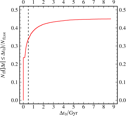
Figure 16: The fraction of large spin flip events that have a major merger within a time $|\Delta t|\leq\Delta t_{0}$. Our dynamical timescale value of $\tau=0.5\,\mathrm{Gyr}$ is marked with a dashed line.

We analyse the inner flips in the same way (Figs. 17 & 18), based on the event distribution shown in Fig. 11. The histogram shows that in this case there are far fewer major mergers following large inner spin flips: $73\%$ ($1928$) of the inner flips associated with a major merger at any time are preceded by the merger, compared to $250$ that are followed by the merger. This is what we would expect: a merger would be initially seen for the halo as a whole, with the inner halo dynamics reacting a short time later. From the cumulative plot (Fig. 18), we can see that just $26.5\%$ of large inner flips have total-halo major mergers at any time before or after. As can also be seen in Figs. 12 & 13, only $4.6\%$ of flips ($455$) coincide exactly with a major merger. If we allow for a time lag between a major merger and the inner halo spin direction changing, then we find $10.7\%$ of flips ($1065$ events) have a merger within $\pm 0.5\,\mathrm{Gyr}$, rising to $17.6\%$ ($1745$ events) within $\pm 1\,\mathrm{Gyr}$.

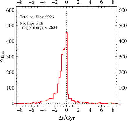
Figure 17: Number of large flips of the inner halo angular momentum that have a (total-halo) major merger a certain amount of time after ($\Delta t>0$) or before ($\Delta t<0$) the flip.

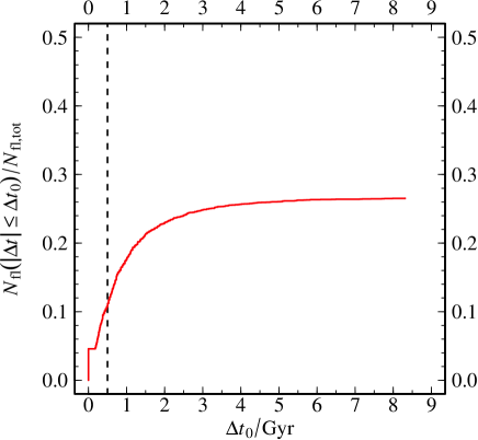
Figure 18: The fraction of inner-halo flip events that have a total-halo major merger within a time $|\Delta t|\leq\Delta t_{0}$.

3.4 Spin flips over halo lifetimes

As in Paper I, we now move on to investigate the likelihood of large spin flips occurring over the lifetimes of haloes, rather than the simple distribution of events discussed in the previous sections. We wish to find the probability of a halo undergoing a spin flip of a given magnitude ($\theta_{0}$) and duration ($\tau$, the event timescale), at some point during its lifetime (excluding events at timesteps when the angular momentum measurement is not reliable). We can also divide this into spin flips during which the halo’s mass does or does not grow by a certain amount, $\Delta\mu_{0}$ (i.e. considering just flips that do or do not coincide with major mergers).

We show the results for this in Fig. 19. As one might expect, as larger timescales $\tau$ are considered, the likelihood of a halo exhibiting a flip of any given size increases. For our fiducial values of $\theta_{0}=45\degr$ and $\tau=0.5\,\mathrm{Gyr}$, we find that $37.8\%$ of the $40\,559$ selected haloes exhibit such a flip at some point in their lives. If we consider just those flips that coincide (exactly) with major mergers, this figure is much lower, at $8.3\%$ (see middle panel). Considering just flips that do not coincide with major mergers (right panel), we find that $34.5\%$ of haloes experience such flips.

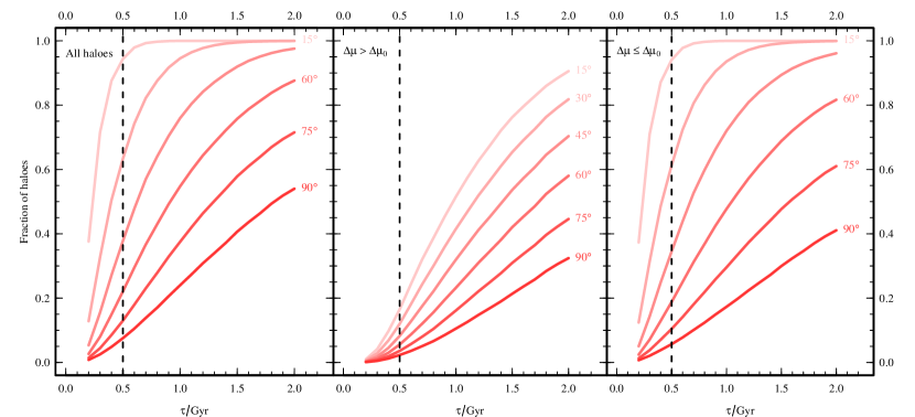
Figure 19: Left: fraction of all halo evolutionary tracks that have at least one spin flip of duration $\tau$ and size $\geq\theta_{0}$. Six values of $\theta_{0}$ have been chosen, every $15\degr$ from $15\degr$ to $90\degr$. Middle: fraction of halo tracks with at least one spin flip that coincides with a major merger. Right: same, but for spin flips that do not coincide with a major merger. The characteristic timescale used in the rest of the paper, $\tau=0.5\,\mathrm{Gyr}$, is marked with a dashed line.

We perform the same analysis for flips of the inner halo angular momentum in Fig. 20. In this case, haloes are more likely to experience inner spin flips of any magnitude and any duration: $64.1\%$ of the $12\,171$ selected haloes have inner flips of at least $45\degr$ over $0.5\,\mathrm{Gyr}$ during the course of their lifetime. As we have seen, fewer inner halo flips coincide with major mergers (e.g. Fig. 18). It is therefore not surprising that, when considering just inner flips that coincide with major mergers, we get a lower fraction of haloes ($3.3\%$) compared to that for the total halo angular momentum.

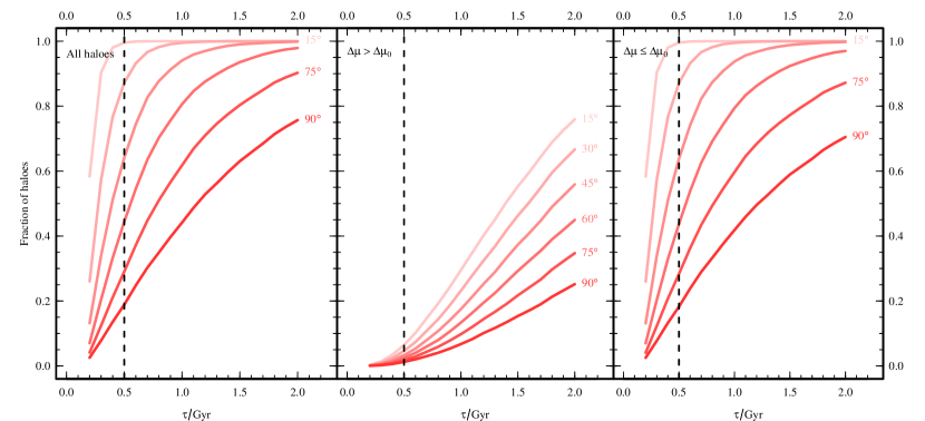
Figure 20: Fraction of all halo tracks that have at least one inner spin flip of at least $\theta_{0}$ and duration $\tau$ (left), and the fractions that have such an inner flip that coincides with a major merger (middle) or does not (right). The same six values of $\theta_{0}$ are used as in the previous figure. The charactersitic timescale used in the rest of the paper, $\tau=0.5\,\mathrm{Gyr}$, is marked with a dashed line.

Since we have haloes over a wide range of final-time masses (both for those that survive to $z=0$ and the ‘doomed’ haloes), it is interesting to ask whether there is any mass-dependence in the probability of flips over halo a lifetime. In Fig. 21, we show this, in a plot analogous to Fig. 19. In this case, instead of plotting results for different spin flip sizes, we set $\theta_{0}=45\degr$ and give the results for different bins of final halo mass.

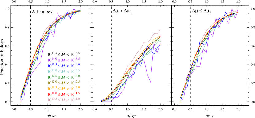
Figure 21: Left: fraction of all halo evolutionary tracks that have at least one spin flip of duration $\tau$ and amplitude $\geq 45\degr$. The middle and right panels also require that the flip does or does not coincide with a major merger (as in Fig. 19). The haloes are divided into bins according to their final-time mass, colour-coded as shown (the masses in the legend are in $\,h^{-1}\mathrm{M}_{\sun}$). An additional dotted heavy black line shows the results over the whole mass range (this is the same as the $45\degr$ line in Fig. 19). Note that the content of the lowest mass bin is affected by our particle-number limit for halo selection: $1000m_{\mathrm{p}}\approx 10^{10.98}\,h^{-1}\mathrm{M}_{\sun}$, and the bin upper limit of $10^{11}\,h^{-1}\mathrm{M}_{\sun}$ corresponds to about $1050$ particles. The timescale used in the rest of the paper, $\tau=0.5\,\mathrm{Gyr}$, is marked with a dashed line.

There is a hint of mass-dependence in the probability for flips: lower-mass haloes appear slightly more likely to experience a flip of a given timescale during their lifetime. This trend is reversed when considering flips of the inner halo angular momentum, shown in Fig. 22. In this case, haloes with larger masses at their final timestep are more likely than lower-mass haloes to have experienced an inner spin flip at some point in their lifetimes. However, in both the total-halo and inner-halo cases, the differences between different mass bins are very slight, and the results from the high mass bins in particular are noisy because they contain relatively few haloes. What trend there is appears stronger when looking at inner flips of short duration, but is broadly consistent over all values of $\tau$ for the total-halo spin flips.

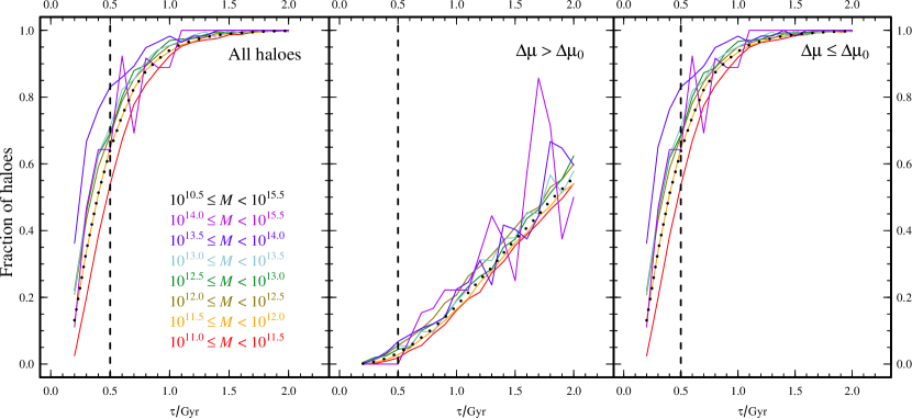
Figure 22: As Fig. 21, but considering flips in the inner halo spin (left), which do (middle) or do not (right) coincide with major mergers. The bins in total-halo final time mass are colour-coded as shown (the masses in the legend are in $\,h^{-1}\mathrm{M}_{\sun}$), with an additional heavy black dotted line showing the results over the whole mass range (as in Fig. 20).

3.5 The contribution of other progenitors

Halo models are commonly used to study the evolution and statistical properties of structures, both in the context of galaxy formation and cosmology in general, such as through Halo Occupation Distribution models (Benson et al., 2000; Berlind & Weinberg, 2002) or the Extended Press–Schechter formalism (e.g. Jiang & van den Bosch, 2014, and references therein). In such models, the evolution of halo properties such as mass is usually assumed to be solely due to mergers with other haloes. For example, the mass of a halo at one timestep is equal to the sum of the masses of its immediate progenitors at the preceding timestep. Similarly, since angular momentum is a conserved quantity, one might assume in such models that the halo angular momentum vector is also equal to the sum of the angular momenta of its immediate progenitor haloes. Here, we are able to test the extent to which this assumption holds for the haloes and merger trees we have defined. We illustrate the relationship between immediate progenitors and halo tracks in Fig. 23; in this section we will be measuring changes in halo properties between a halo at a given timestep and the sum of the property over its immediate progenitors. We consider just the root tracks, to avoid double-counting haloes as end-points of one track and progenitors of another. We also use each simulation snapshot output, rather than interpolating between snapshots to get a constant timescale $\tau$ as in the previous sections.

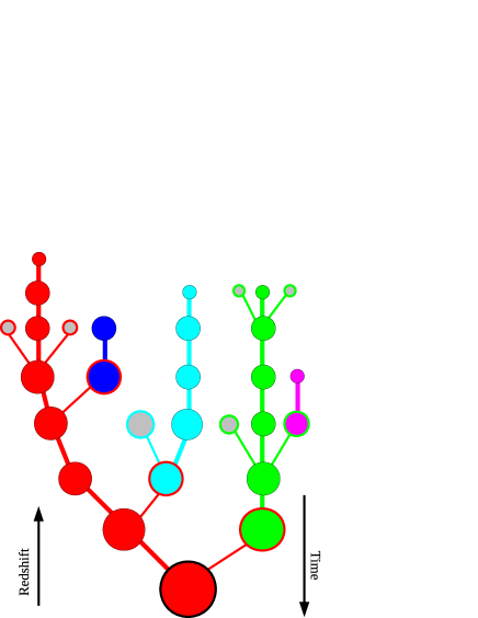
Figure 23: Schematic of a single merger tree, showing immediate progenitors of evolutionary tracks (cf. Fig. 1). The circles represent haloes in the tree at different timesteps. Each evolutionary track is given an individual colour (although ‘tracks’ that only exist for a single timestep are all coloured grey). Haloes at the end-point of their tracks have a heavy outline. When a halo is an immediate progenitor of a halo from a different track, it has that track’s colour as an outline.

We compute the fractional mass change between a halo at time $t_{i}$ and the sum of the masses of its $N_{\mathrm{prog}}$ immediate progenitors identified at the preceding timestep, $t_{i-1}$:

$$\Delta\mu_{\mathrm{pr}}(t_{i}):=\frac{M(t_{i})-\sum_{p=1}^{N_{\mathrm{prog}}}M_{p}(t_{i-1})}{M(t_{i})}.$$ (4)

We can also compute the centre-of-momentum frame for the set of progenitors, and thus their total angular momentum vector in that frame $\textbf{{J}}_{\mathrm{progs}}=\sum_{p=1}^{N_{\mathrm{prog}}}\textbf{{J}}_{p}$. We can therefore calculate the change in orientation between that total angular momentum of the progenitors and the subsequent halo angular momentum,

$$\cos\phi(t_{i}):=\frac{\textbf{{J}}(t_{i})\mathbf{\cdot}\textbf{{J}}_{\mathrm{progs}}(t_{i-1})}{\left|\textbf{{J}}(t)\right|\left|\textbf{{J}}_{\mathrm{progs}}(t_{i-1})\right|}.$$ (5)

In Fig. 24, we plot the joint distribution of events in terms of $\cos\phi$ and $\Delta\mu_{\mathrm{pr}}$ (subject to the same standard selection criteria as before, see section 2.3), along with associated histograms (by analogy to our previous figures).

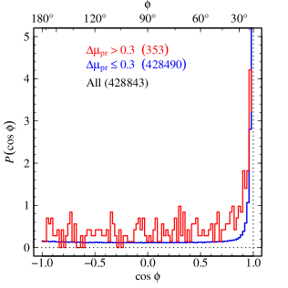
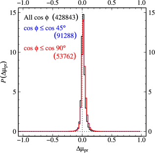
Figure 24: Left: joint distribution of the fractional mass change and spin orientation change between haloes at a given timestep and their progenitors at the immediately preceding timestep. Middle: histogram showing the distribution across $\cos\phi$, for all events (black), and those when there is a large additional change in mass (red), and when there is not (blue). Right: histogram showing the cross-section through the joint distribution as a function of $\Delta\mu_{\mathrm{pr}}$, for all events (black), and events when the total spin changes by at least $45\degr$ (blue) and $90\degr$ (red).

From these figures, we can see that the assumption that mass is conserved between haloes and their progenitors is quite well-founded, i.e. $\Delta\mu_{\mathrm{pr}}\approx 0$. There are relatively few events with large values of $|\Delta\mu_{\mathrm{pr}}|$, with over $84\%$ of the events located within $|\Delta\mu_{\mathrm{pr}}|<0.05$.

The angular momentum orientation behaves differently. Although it cannot be seen clearly in the joint distribution image (left panel of Fig. 24), the histogram of $\cos\phi$ (middle panel) shows that there is a very strong peak at no change; we find that $40\%$ of the events involve orientation changes of less than $5\degr$. However, there appears to be an almost uniform probability for a change in the orientation of the halo spin with respect to its immediate progenitors, as long as the change is $\phi\ga 45\degr$. Note that, as mentioned earlier, multiple rapid mergers (between two snapshots) could result in rather chaotic changes in spin direction, as the result depends on the details of the spins and accretion directions of the merging objects. The necessity of using discrete output times means that our results can be seen as a lower limit, and could be quantitatively different with different time resolutions.

Thus, while halo mass is reasonably well conserved between timesteps, angular momentum is not. This is in agreement with Book et al. (2011), who studied the evolution of angular momentum of individual haloes and their particles in detail.

4 Conclusions

In this paper, we have investigated the frequency of changes in the spin direction of dark matter haloes over their lifetimes, and how such changes relate to the halo merger history. In a simple halo model, one might assume that large, sudden changes in spin direction – spin flips – occur exclusively during major mergers, with the angular momentum direction remaining relatively stable during intervening times. Extending the work of Bett & Frenk (2012), we have shown that this is not the case for haloes with final masses spanning $\sim 10^{11}$ – $10^{15}\,h^{-1}\mathrm{M}_{\sun}$, with spin flips, in fact, occurring often without major mergers.

We find that $39\%$ of major mergers coincide with spin flips of $45\degr$ or more. Minor mergers or accretion events are very unlikely to coincide with such flips: just $2\%$ of non-major-merger events do so. However, the shape of the joint distribution of fractional mass change, $\Delta\mu$, and spin orientation change, $\cos\theta$, is such that large spin flips are very likely to coincide with non-major-merger events; $76\%$ of spin flips do so.

Changes in spin direction correlate poorly with changes in specific angular momentum magnitude. Spin flips coincide with a broad range of changes in specific angular momentum, albeit with a slight preference for an increase with large flips.

If we consider only those haloes that survive to $z=0$, then we find that the joint distribution of $\Delta\mu$ and $\cos\theta$ is noticably narrower in $\Delta\mu$: haloes that are doomed to merge into another halo before $z=0$ have many more mass-loss events ($\Delta\mu<0$). This is probably a feature of the merger trees we are using, with haloes losing mass before the timestep at which they cease to be recognised as an independent halo. For those haloes that do survive to $z=0$, we find that less than $1\%$ of minor mergers coincide with large spin flips, but over $95\%$ of large flips coincide with minor mergers.

Since changes in the inner regions of a halo are more likely to have a strong impact on the evolution of the central galaxy, we have also investigated the relationship between flips in the inner halo spin and mergers in the halo as a whole. In this case, we find that there is a general increase in the probability of a spin flip. In particular over $95\%$ of large inner flips coincide with minor mergers (over $99\%$ for the haloes that survive to $z=0$), and $6.3\%$ of minor mergers coincide with a large inner flip.

Many of those large flips that coincide with minor mergers do in fact have a major merger associated with them – but at a slightly earlier or later timestep. We have investigated the number of large flip events that have a major merger within a given time window $\Delta t$, and while major mergers can occur before or after large flips, there is a tendency for major mergers to precede the flip. However, even allowing for these inexact conincidences of major mergers and flips, most large flips nevertheless are never associated with a major merger, even when $\Delta t$ is extended to several gigayears.

As in Paper I, we have also considered the likelihood of a large spin flip occurring over the lifetime of a halo, in addition to the distribution of flip events. We find that $37.5\%$ of haloes undergo flips of at least $45\degr$ over a timescale of $0.5\,\mathrm{Gyr}$ ($64.1\%$ for inner-halo flips). Furthermore, despite the broad range of final masses for the haloes we consider ($\sim 10^{11}$–$10^{15}$), there is little sign of any significant trend in these results with halo mass.

Finally, we have tested how well-conserved halo properties are when going from the set of immediate progenitors at one timestep to the single resulting halo at the next timestep. Halo models usually assume that halo mass is conserved during mergers (i.e. that the sum of masses of the progenitors equals the mass of the resulting halo), and we find that this is a reasonably good approximation. One might also imagine that the resultant halo’s angular momentum is equal to the (vector) sum of those of its immediate progenitors. However, we do not find this to be the case. Although $40\%$ of events do have no orientation change between the net spin of progenitors and the final halo spin, the distribution in this orientation change becomes uniform for changes greater than about $45\degr$ – i.e. all post-merger orientations greater than $45\degr$ are equally probable.

Our findings have consequences for the use of simple halo models, both in theoretical studies and when interpreting observations. Care must be taken when making modelling assumptions related to angular momentum in various contexts. These include the relationship between angular momentum and galaxy morphology; the orientation and persistence of the orientation of haloes with respect to galaxies, and with respect to larger-scale structures; and studies that relate dynamical disturbance solely to galaxy mergers.

The present study has not addressed the cause of the non-major-merger spin flips that we have observed (although they are presumably related to flybys of satellite haloes, or similar phenomena), and it would be interesting to relate them to properties of the immediate environment of the halo in question. Although we have treated mergers (and for the most part, spin flips) as discrete instantaneous events (albeit with a given timescale $\tau$), with higher time resolution one would hope to be able to resolve the merger or flip process itself and be able to measure their timescales directly.

While our choce of algorithms for merger tree, halo definition and selection will have quantitatively affected our results, qualitatively speaking the work presented here can be seen as a warning against using oversimplified halo models of structure and galaxy formation. Haloes can clearly be disturbed by processes related to, but separate from, simply their mass accretion history. Incorporating additional halo properties such as spin direction in models of galaxy formation – perhaps by tracking spin vectors in addition to halo mass – can prove a useful approach to improving their ability to match the observed universe.

Due to the difficulties in robustly resolving spin changes in simulations (which motivated our series of selection criteria), Padilla et al. (2014) took a statistical approach when implementing spin direction changes in their semi-analytic model, rather than tracking halo spin vectors directly. Further studies of the statistics of spin flips should be carried out in simulations that resolve the dynamics of structures on different scales (at higher resolution, and at larger scales), to improve and constrain the implementation of spin flips in semi-analytic galaxy formation models.

Appendix A Choice of halo event timescale

We wish to find an appropriate characteristic timescale of haloes to use for calculating changes in halo properties. While we expect such a timescale to depend on cosmology, redshift, and halo mass, we aim to find a single value that we can use throughout our analysis. We will compare our results at different timescales to demonstrate the degree to which they depend on this choice of timescale.

In general, we can write a timescale as $\tau=\ell/v$. We take the characteristic length $\ell$ to be some multiple of a characteristic halo radius $yr$, where for example $y=2$, $\pi$, $2\pi$, etc, making $\ell$ the diameter, circumference, etc. We take the characteristic velocity $v$ to be the circular velocity of a test particle at $r$ orbiting under gravity, $v=\sqrt{GM(<r)/r}$. The timescale is therefore given by

$$\tau=y\sqrt{\frac{r^{3}}{GM(<r)}}.$$ (6)

If we model a halo as the mass within a particular spherical boundary set by an overdensity criterion, and we take $r=R_{\mathrm{vir}}$, then $M(<r)\equiv M_{\mathrm{vir}}=\frac{4}{3}\pi R_{\mathrm{vir}}^{3}\Delta_{\mathrm{c}}(z)\,\rho_{\mathrm{crit}}(z)$. Defining for convenience $\chi(z)=\Omega_{\mathrm{M}0}a^{-3}+\Omega_{\Lambda 0}$, we can write $\rho_{\mathrm{crit}}=\chi(z)\,\rho_{\mathrm{crit,}0}=\chi(z)\,3H_{0}^{2}/8\pi G$, giving

$$\tau(z)=y\sqrt{\frac{3}{4\pi G}\frac{8\pi G}{3H_{0}^{2}}\frac{1}{\chi(z)\Delta_{\mathrm{c}}(z)}}\,\equiv\frac{y}{H_{0}}\sqrt{\frac{2}{\chi(z)\Delta_{\mathrm{c}}(z)}}.$$ (7)

Since our definition of $R_{\mathrm{vir}}$ depends only on cosmology and time, so also does $\tau$ – losing any dependence on halo properties, making it a cosmological timescale rather than a halo timescale. In fact, since the overdensity criterion, $\Delta_{\mathrm{c}}(z)$, originates in the spherical collapse model of halo formation, this timescale is that of the haloes that are forming at redshift $z$, rather than of the spectrum of extant haloes at that redshift.

An alternative is to take the characteristic radius somewhere within $R_{\mathrm{vir}}$, thus incorporating the halo density profile and retaining some dependence on halo scale and history. If we take the characteristic radius as that enclosing some fraction of the halo mass, i.e. $f_{\mathrm{M}}=M(<R_{f})/M_{\mathrm{vir}}$, and $r=R_{f}$, then equation (6) becomes:

$$\tau = y\sqrt{\frac{R_{f}^{3}}{Gf_{\mathrm{M}}M_{\mathrm{vir}}}}$$ (8)

$$= y\sqrt{\frac{3}{4\pi G}\frac{8\pi G}{3H_{0}^{2}}\frac{R_{f}^{3}}{f_{\mathrm{M}}R_{\mathrm{vir}}^{3}}\frac{1}{\chi(z)\Delta_{\mathrm{c}}(z)}}$$ (9)

$$= \frac{y}{H_{0}}\sqrt{\frac{R_{f}^{3}}{f_{\mathrm{M}}R_{\mathrm{vir}}^{3}}\frac{2}{\chi(z)\Delta_{\mathrm{c}}(z)}}$$ (10)

We now assume an NFW density profile (Navarro et al., 1996, 1997),

$$\rho(r)=\frac{\rho_{\mathrm{s}}}{\frac{r}{r_{\mathrm{s}}}\left(1+\frac{r}{r_{\mathrm{s}}}\right)^{2}}$$ (11)

where the halo concentration is related to the scale radius through $c=R_{\mathrm{vir}}/r_{\mathrm{s}}$ and the characteristic density is

$$\rho_{\mathrm{s}}=\frac{\Delta_{\mathrm{c}}\rho_{\mathrm{crit}}}{3}\frac{c^{3}}{\left(\ln\left(1+c\right)-\frac{c}{1+c}\right)}.$$ (12)

The cumulative mass is $M(<R)=4\pi\int^{R}_{0}\rho(r)r\;\mathrm{d}r$, so here

$$M(<R)=4\pi\rho_{\mathrm{s}}\int^{R}_{0}\frac{r^{2}}{\frac{r}{r_{\mathrm{s}}}\left(1+\frac{r}{r_{\mathrm{s}}}\right)^{2}}\mathrm{d}r.$$ (13)

If we define $x=r/R_{\mathrm{vir}}$ so that $cx=r/r_{\mathrm{s}}$, we get

$$M(<R_{\mathrm{vir}})=4\pi\rho_{\mathrm{s}}\frac{R_{\mathrm{vir}}^{3}}{c^{3}}\left(\ln(1+cx)-\frac{cx}{1+cx}\right)$$ (14)

$$=\frac{4}{3}\pi R_{\mathrm{vir}}^{3}\Delta_{\mathrm{c}}(z)\rho_{\mathrm{crit}}(z)\left(\frac{\ln(1+cx)-\frac{cx}{1+cx}}{\ln(1+c)-\frac{c}{1+c}}\right)$$ (15)

The radius fraction, $x$, for a given concentration can then be found by solving

$$\ln(1+cx)-\frac{cx}{1+cx}=f_{\mathrm{M}}\left(\ln(1+c)-\frac{c}{1+c}\right).$$ (16)

In the case of $f_{\mathrm{M}}=1/2$, Łokas & Mamon (2001) provided a fitting formula for $x(c)$ and thus the half-mass radius, $R_{1/2}$.

To link this back to the halo mass and radius, we need a concentration–mass relation for all redshifts; fitting formulae for such a relation are provided, for example, in Muñoz-Cuartas et al. (2011). So, for a given halo mass and desired fraction $f_{\mathrm{M}}$, at a given redshift, we can find a concentration and thus $x=R_{f}/R_{\mathrm{vir}}$, and finally $\tau$.

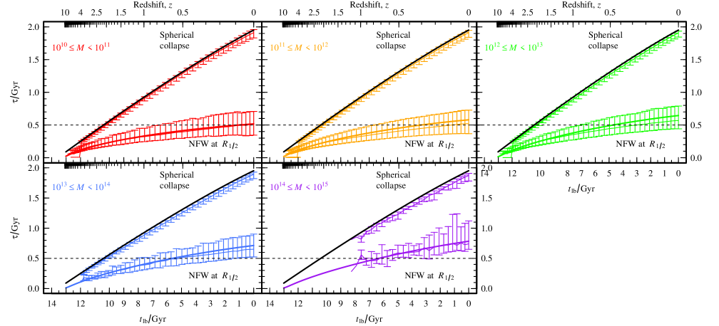
Figure 25: Different halo timescales as a function of lookback time, $t_{\mathrm{lb}}$, with each panel showing haloes of different masses at each snapshot. The lines labelled ‘Spherical collapse’ use the halo-independent timescale: The analytic result from equation (7) (solid black line) is compared to the medians and 10th/90th percentiles (points & error bars) from the distribution of measured timescales from the haloes at each snapshot, using equation (6) with $r=R_{\mathrm{vir}}$. The data labelled ‘NFW at $R_{1/2}$’ shows the timescale at the half-mass radius: the solid lines are from equation (10) with $f_{\mathrm{M}}=1/2$, assuming an NFW profile and using the fitting formulae (see text; Muñoz-Cuartas et al. 2011, Łokas & Mamon 2001). The points again show the medians and percentiles of the measured timescale (equation (6) with $r=R_{1/2}$) from haloes in mass bins at each snapshot.

Fig. 25 shows the timescales from the above equations (7) and (10) (in the latter taking $f_{\mathrm{M}}=1/2$ so $R_{f}=R_{1/2}$), along with the timescales measured from haloes at each timestep using $\tau_{\mathrm{meas}}=\sqrt{R_{\mathrm{vir}}^{3}/(GM_{\mathrm{h}})}$ and $\tau_{1/2,\mathrm{meas}}=\sqrt{2R_{1/2}^{3}/(GM_{\mathrm{h}})}$. (Haloes are selected in this case only if they have at least $1000$ particles.) The results from the haloes themselves match the analytic results very well in all cases. Given the mass distribution of our haloes over the time period of interest, we opt to use a single value of $\tau=0.5\,\mathrm{Gyr}$ for analysing halo property changes. Using a single value makes for more straightforward comparisons and analysis as haloes grow and evolve, and the results presented above show that this is a reasonable approximation for our haloes.

We expect the choice of timescale to affect our results quantitatively, but not qualitatively. While some of our results are already shown as a function of measurement timescale (see section 3.4), we show here how the event distribution varies with the choice of $\tau$. Fig. 26 compares the event distribution from Fig. 2 (i.e. using $\tau=0.5\,\mathrm{Gyr}$), with that obtained when values of $\tau=0.3\,\mathrm{Gyr}$ and $1.0\,\mathrm{Gyr}$ are used, and when just the (variable) inter-snapshot timestep is used. These show that, in practice, there is very little difference between the universal timescale we choose and just looking at property differences between snapshots. In contrast, using a longer timescale produces a broader distribution, with more events spread away from the ‘no change’ point, and using a shorter timescale produces a tighter distribution. It seems that spin orientation change $\cos\theta$ is affected more than the fractional mass change $\Delta\mu$.

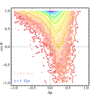
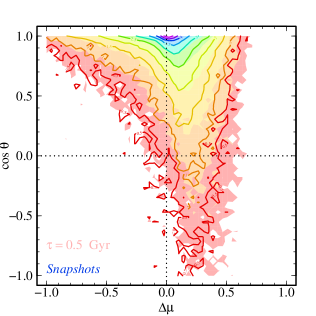
Figure 26: Contour plots of event distributions following that of Fig. 2. Those results are shown as filled contours. The outline contours show the results of varying the choice of $\tau$, with the left panel using a shorter timescale, the middle panel using a longer timescale. The right panel uses the time difference between the simulation snapshots directly, without interpolation (i.e. a variable timescale between $~{}0.4\,\mathrm{Gyr}$ and $0.1\,\mathrm{Gyr}$.). The same selection criteria as in Fig. 2 are used in all cases.

References

- Agustsson & Brainerd (2010) Agustsson I., Brainerd T. G., 2010, ApJ, 709, 1321
- Allgood et al. (2006) Allgood B., Flores R. A., Primack J. R., Kravtsov A. V., Wechsler R. H., Faltenbacher A., Bullock J. S., 2006, MNRAS, 367, 1781
- Aumer & White (2013) Aumer M., White S. D. M., 2013, MNRAS, 428, 1055
- Avila-Reese et al. (2005) Avila-Reese V., Colín P., Gottlöber S., Firmani C., Maulbetsch C., 2005, ApJ, 634, 51
- Avila et al. (2014) Avila S., et al., 2014, MNRAS, 441, 3488
- Bailin & Steinmetz (2005) Bailin J., Steinmetz M., 2005, ApJ, 627, 647
- Barnes (1988) Barnes J. E., 1988, ApJ, 331, 699
- Barnes (1992) Barnes J. E., 1992, ApJ, 393, 484
- Barnes & Hernquist (1996) Barnes J. E., Hernquist L., 1996, ApJ, 471, 115
- Baugh (2006) Baugh C. M., 2006, Rep. Prog. Phys., 69, 3101
- Benson (2010) Benson A. J., 2010, Phys. Rep., 495, 33
- Benson et al. (2000) Benson A. J., Cole S., Frenk C. S., Baugh C. M., Lacey C. G., 2000, MNRAS, 311, 793
- Berlind & Weinberg (2002) Berlind A. A., Weinberg D. H., 2002, ApJ, 575, 587
- Bett (2010) Bett P. E., 2010, in V. P. Debattista & C. C. Popescu ed., AIP Conf. Ser. Vol. 1240, Hunting for the Dark: The Hidden Side of Galaxy Formation. Am. Inst. Phys., New York, pp 403–404 (arXiv:0912.4605), doi:10.1063/1.3458546
- Bett & Frenk (2012) Bett P. E., Frenk C. S., 2012, MNRAS, 420, 3324
- Bett et al. (2007) Bett P., Eke V., Frenk C. S., Jenkins A., Helly J., Navarro J., 2007, MNRAS, 376, 215
- Bett et al. (2010) Bett P., Eke V., Frenk C. S., Jenkins A., Okamoto T., 2010, MNRAS, 404, 1137
- Book et al. (2011) Book L. G., Brooks A., Peter A. H. G., Benson A. J., Governato F., 2011, MNRAS, 411, 1963
- Bournaud et al. (2005) Bournaud F., Jog C. J., Combes F., 2005, A&A, 437, 69
- Bower et al. (2006) Bower R. G., Benson A. J., Malbon R., Helly J. C., Frenk C. S., Baugh C. M., Cole S., Lacey C. G., 2006, MNRAS, 370, 645
- Boylan-Kolchin et al. (2009) Boylan-Kolchin M., Springel V., White S. D. M., Jenkins A., Lemson G., 2009, MNRAS, 398, 1150
- Brunino et al. (2007) Brunino R., Trujillo I., Pearce F. R., Thomas P. A., 2007, MNRAS, 375, 184
- Bryan & Norman (1998) Bryan G. L., Norman M. L., 1998, ApJ, 495, 80
- Bullock et al. (2001) Bullock J. S., Dekel A., Kolatt T. S., Kravtsov A. V., Klypin A. A., Porciani C., Primack J. R., 2001, ApJ, 555, 240
- Catelan & Theuns (1996a) Catelan P., Theuns T., 1996a, MNRAS, 282, 436
- Catelan & Theuns (1996b) Catelan P., Theuns T., 1996b, MNRAS, 282, 455
- Chen et al. (2003) Chen D. N., Jing Y. P., Yoshikawa K., 2003, ApJ, 597, 35
- Codis et al. (2012) Codis S., Pichon C., Devriendt J., Slyz A., Pogosyan D., Dubois Y., Sousbie T., 2012, MNRAS, 427, 3320
- Codis et al. (2015) Codis S., Pichon C., Pogosyan D., 2015, MNRAS, 452, 3369
- Cox et al. (2006) Cox T. J., Dutta S. N., Di Matteo T., Hernquist L., Hopkins P. F., Robertson B., Springel V., 2006, ApJ, 650, 791
- Cox et al. (2008) Cox T. J., Jonsson P., Somerville R. S., Primack J. R., Dekel A., 2008, MNRAS, 384, 386
- Croft et al. (2009) Croft R. A. C., Di Matteo T., Springel V., Hernquist L., 2009, MNRAS, 400, 43
- Cuesta et al. (2008) Cuesta A. J., Betancort-Rijo J. E., Gottlöber S., Patiri S. G., Yepes G., Prada F., 2008, MNRAS, 385, 867
- Davis et al. (1985) Davis M., Efstathiou G., Frenk C. S., White S. D. M., 1985, ApJ, 292, 371
- De Lucia & Blaizot (2007) De Lucia G., Blaizot J., 2007, MNRAS, 375, 2
- Deason et al. (2011) Deason A. J., et al., 2011, MNRAS, 415, 2607
- Doroshkevich (1970a) Doroshkevich A. G., 1970a, Astrophysics, 6, 320
- Doroshkevich (1970b) Doroshkevich A. G., 1970b, Afz, 6, 581
- Dubois et al. (2014) Dubois Y., et al., 2014, MNRAS, 444, 1453
- Eke et al. (1996) Eke V. R., Cole S., Frenk C. S., 1996, MNRAS, 282, 263
- Fakhouri & Ma (2008) Fakhouri O., Ma C., 2008, MNRAS, 386, 577
- Fakhouri & Ma (2009) Fakhouri O., Ma C., 2009, MNRAS, 394, 1825
- Fall & Efstathiou (1980) Fall S. M., Efstathiou G., 1980, MNRAS, 193, 189
- Gao et al. (2008) Gao L., Navarro J. F., Cole S., Frenk C. S., White S. D. M., Springel V., Jenkins A., Neto A. F., 2008, MNRAS, 387, 536
- Genel et al. (2009) Genel S., Genzel R., Bouché N., Naab T., Sternberg A., 2009, ApJ, 701, 2002
- Gustafsson et al. (2006) Gustafsson M., Fairbairn M., Sommer-Larsen J., 2006, Phys. Rev. D, 74, 123522
- Hahn et al. (2007a) Hahn O., Porciani C., Carollo C. M., Dekel A., 2007a, MNRAS, 375, 489
- Hahn et al. (2007b) Hahn O., Carollo C. M., Porciani C., Dekel A., 2007b, MNRAS, 381, 41
- Hahn et al. (2010) Hahn O., Teyssier R., Carollo C. M., 2010, MNRAS, 405, 274
- Harker et al. (2006) Harker G., Cole S., Helly J., Frenk C., Jenkins A., 2006, MNRAS, 367, 1039
- Hayashi et al. (2007) Hayashi E., Navarro J. F., Springel V., 2007, MNRAS, 377, 50
- Hernquist (1992) Hernquist L., 1992, ApJ, 400, 460
- Hernquist (1993) Hernquist L., 1993, ApJ, 409, 548
- Hopkins et al. (2009a) Hopkins P. F., et al., 2009a, MNRAS, 397, 802
- Hopkins et al. (2009b) Hopkins P. F., Cox T. J., Younger J. D., Hernquist L., 2009b, ApJ, 691, 1168
- Hopkins et al. (2010) Hopkins P. F., et al., 2010, ApJ, 715, 202
- Hoyle (1951) Hoyle F., 1951, in Burgers J. M., van de Hulst H. C., eds, Problems of Cosmical Aerodynamics. Central Air Documents Office, Dayton, OH, pp 195–197
- Jiang & van den Bosch (2014) Jiang F., van den Bosch F. C., 2014, MNRAS, 440, 193
- Jiang et al. (2014) Jiang L., Helly J. C., Cole S., Frenk C. S., 2014, MNRAS, 440, 2115
- Knebe & Power (2008) Knebe A., Power C., 2008, ApJ, 678, 621
- Knebe et al. (2013) Knebe A., et al., 2013, MNRAS, 435, 1618
- Lemson & the Virgo Consortium (2006) Lemson G., the Virgo Consortium 2006, preprint, (arXiv:astro-ph/0608019)
- Libeskind et al. (2009) Libeskind N. I., Frenk C. S., Cole S., Jenkins A., Helly J. C., 2009, MNRAS, 399, 550
- Libeskind et al. (2012) Libeskind N. I., Hoffman Y., Knebe A., Steinmetz M., Gottlöber S., Metuki O., Yepes G., 2012, MNRAS, 421, L137
- Łokas & Mamon (2001) Łokas E. L., Mamon G. A., 2001, MNRAS, 321, 155
- Macciò et al. (2007) Macciò A. V., Dutton A. A., van den Bosch F. C., Moore B., Potter D., Stadel J., 2007, MNRAS, 378, 55
- Macciò et al. (2008) Macciò A. V., Dutton A. A., van den Bosch F. C., 2008, MNRAS, 391, 1940
- Maller et al. (2006) Maller A. H., Katz N., Kereš D., Davé R., Weinberg D. H., 2006, ApJ, 647, 763
- Mo et al. (1998) Mo H. J., Mao S., White S. D. M., 1998, MNRAS, 295, 319
- Moster et al. (2010) Moster B. P., Macciò A. V., Somerville R. S., Johansson P. H., Naab T., 2010, MNRAS, 403, 1009
- Muñoz-Cuartas et al. (2011) Muñoz-Cuartas J. C., Macciò A. V., Gottlöber S., Dutton A. A., 2011, MNRAS, 411, 584
- Naab & Burkert (2003) Naab T., Burkert A., 2003, ApJ, 597, 893
- Navarro et al. (1996) Navarro J. F., Frenk C. S., White S. D. M., 1996, ApJ, 462, 563
- Navarro et al. (1997) Navarro J. F., Frenk C. S., White S. D. M., 1997, ApJ, 490, 493
- Neistein et al. (2010) Neistein E., Macciò A. V., Dekel A., 2010, MNRAS, 403, 984
- Neto et al. (2007) Neto A. F., et al., 2007, MNRAS, 381, 1450
- Okamoto et al. (2005) Okamoto T., Eke V. R., Frenk C. S., Jenkins A., 2005, MNRAS, 363, 1299
- Padilla et al. (2014) Padilla N. D., Salazar-Albornoz S., Contreras S., Cora S. A., Ruiz A. N., 2014, MNRAS, 443, 2801
- Paz et al. (2008) Paz D. J., Stasyszyn F., Padilla N. D., 2008, MNRAS, 389, 1127
- Peebles (1969) Peebles P. J. E., 1969, ApJ, 155, 393
- Porciani et al. (2002) Porciani C., Dekel A., Hoffman Y., 2002, MNRAS, 332, 325
- Romano-Díaz et al. (2009) Romano-Díaz E., Shlosman I., Heller C., Hoffman Y., 2009, ApJ, 702, 1250
- Scannapieco et al. (2009) Scannapieco C., White S. D. M., Springel V., Tissera P. B., 2009, MNRAS, 396, 696
- Schäfer (2009) Schäfer B. M., 2009, International Journal of Modern Physics D, 18, 173
- Shaw et al. (2006) Shaw L. D., Weller J., Ostriker J. P., Bode P., 2006, ApJ, 646, 815
- Springel et al. (2001) Springel V., White S. D. M., Tormen G., Kauffmann G., 2001, MNRAS, 328, 726
- Springel et al. (2005) Springel V., et al., 2005, Nature, 435, 629
- Srisawat et al. (2013) Srisawat C., et al., 2013, MNRAS, 436, 150
- Stewart et al. (2008) Stewart K. R., Bullock J. S., Wechsler R. H., Maller A. H., Zentner A. R., 2008, ApJ, 683, 597
- Stewart et al. (2009) Stewart K. R., Bullock J. S., Wechsler R. H., Maller A. H., 2009, ApJ, 702, 307
- Sugerman et al. (2000) Sugerman B., Summers F. J., Kamionkowski M., 2000, MNRAS, 311, 762
- Toomre (1977) Toomre A., 1977, in B. M. Tinsley & R. B. Larson ed., Evolution of Galaxies and Stellar Populations. pp 401–416
- Toomre & Toomre (1972) Toomre A., Toomre J., 1972, ApJ, 178, 623
- Tweed et al. (2009) Tweed D., Devriendt J., Blaizot J., Colombi S., Slyz A., 2009, A&A, 506, 647
- Warren et al. (1992) Warren M. S., Quinn P. J., Salmon J. K., Zurek W. H., 1992, ApJ, 399, 405
- Wechsler et al. (2002) Wechsler R. H., Bullock J. S., Primack J. R., Kravtsov A. V., Dekel A., 2002, ApJ, 568, 52
- Welker et al. (2014) Welker C., Devriendt J., Dubois Y., Pichon C., Peirani S., 2014, MNRAS, 445, L46
- Welker et al. (2015) Welker C., Dubois Y., Devriendt J., Pichon C., Kaviraj S., Peirani S., 2015, preprint, (arXiv:1502.05053)
- White (1984) White S. D. M., 1984, ApJ, 286, 38
- White & Frenk (1991) White S. D. M., Frenk C. S., 1991, ApJ, 379, 52
- White & Rees (1978) White S. D. M., Rees M. J., 1978, MNRAS, 183, 341
- Zavala et al. (2008) Zavala J., Okamoto T., Frenk C. S., 2008, MNRAS, 387, 364
- van den Bosch et al. (2002) van den Bosch F. C., Abel T., Croft R. A. C., Hernquist L., White S. D. M., 2002, ApJ, 576, 21
- van den Bosch et al. (2003) van den Bosch F. C., Abel T., Hernquist L., 2003, MNRAS, 346, 177