EUROPEAN ORGANIZATION FOR NUCLEAR RESEARCH (CERN)

​​​ CERN-PH-EP-2015-272 LHCb-PAPER-2015-041

Measurements of prompt charm production cross-sections in $pp$ collisions at $\sqrt{s}=13$ TeV

The LHCb collaboration

Production cross-sections of prompt charm mesons are measured with the first data from $pp$ collisions at the LHC at a centre-of-mass energy of $13\text{\,}\mathrm{TeV}$. The data sample corresponds to an integrated luminosity of $4.98\pm 0.19\text{\,}{\mathrm{pb}}^{-1}$ collected by the LHCb experiment. The production cross-sections of $D^{0}$, $D^{+}$, $D_{s}^{+}$, and $D^{*+}$ mesons are measured in bins of charm meson transverse momentum, $p_{\mathrm{T}}$, and rapidity, $y$, and cover the range $0<p_{\mathrm{T}}<$15\text{\,}\mathrm{{\mathrm{\,Ge\kern-1.00006ptV\!/}c}}$$ and $2.0<y<4.5$. The inclusive cross-sections for the four mesons, including charge conjugation, within the range of $1<p_{\mathrm{T}}<$8\text{\,}\mathrm{{\mathrm{\,Ge\kern-1.00006ptV\!/}c}}$$ are found to be

$$\begin{array}[]{lcr}\sigma(\mbox{$pp\to D^{0}X$})&=&$2072\pm 2\pm 124\text{\,}\mathrm{\SIUnitSymbolMicro b}$,\\ \sigma(\mbox{$pp\to D^{+}X$})&=&$834\pm 2\pm\phantom{1}78\text{\,}\mathrm{\SIUnitSymbolMicro b}$,\\ \sigma(\mbox{$pp\to D_{s}^{+}X$})&=&$353\pm 9\pm\phantom{1}76\text{\,}\mathrm{\SIUnitSymbolMicro b}$,\\ \sigma(\mbox{$pp\to D^{*+}X$})&=&$784\pm 4\pm\phantom{1}87\text{\,}\mathrm{\SIUnitSymbolMicro b}$,\\ \end{array}$$

where the uncertainties are due to statistical and systematic uncertainties, respectively.

Published in JHEP 03 (2016) 159

Errata published in JHEP 09 (2016) 013 and JHEP 05 (2017) 074

© CERN on behalf of the LHCb collaboration, licence CC-BY-4.0.

 

1 Introduction

Measurements of charm production cross-sections in proton-proton collisions are important tests of the predictions of perturbative quantum chromodynamics [1, 2, 3]. Predictions of charm meson cross-sections have been made at next-to-leading order using the generalized mass variable flavour number scheme (GMVFNS) [4, 5, 6, 7, 8, 3] and at fixed order with next-to-leading-log resummation (FONLL) [1, 9, 10, 11, 12, 2]. These are based on a factorisation approach, where the cross-sections are calculated as a convolution of three terms: the parton distribution functions of the incoming protons; the partonic hard scattering rate, estimated as a perturbative series in the coupling constant of the strong interaction; and a fragmentation function that parametrises the hadronisation of the charm quark into a given type of charm hadron. The range of $y$ and $p_{\mathrm{T}}$ accessible to LHCb enables quantum chromodynamics calculations to be tested in a region where the momentum fraction, $x$, of the initial state partons can reach values below $10^{-4}$. In this region the uncertainties on the gluon parton density functions are large, exceeding 30$\%$ [1, 13], and LHCb measurements can be used to constrain them. For example, the predictions provided in Ref. [1] have made direct use of these constraints from LHCb data, taking as input a set of parton density functions that is weighted to match the LHCb measurements at $\sqrt{s}=$7\text{\,}\mathrm{TeV}$$.

The charm production cross-sections are also important in evaluating the rate of high-energy neutrinos created from the decay of charm hadrons produced in cosmic ray interactions with atmospheric nuclei [14, 1]. Such neutrinos constitute an important background for experiments such as IceCube [15] searching for neutrinos produced from astrophysical sources. The previous measurements from LHCb at $\sqrt{s}=$7\text{\,}\mathrm{TeV}$$ [16] permit the evaluation of this background for incoming cosmic rays with energy of $26\text{\,}\mathrm{\mathrm{\,Pe\kern-1.00006ptV}}$. In this paper measurements at $\sqrt{s}=$13\text{\,}\mathrm{TeV}$$ are presented, probing a new kinematic region that corresponds to a primary cosmic ray energy of $90\text{\,}\mathrm{\mathrm{\,Pe\kern-1.00006ptV}}$.

Measurements of the charm production cross-sections have been performed in different kinematic regions and centre-of-mass energies. Measurements by the CDF experiment cover the central rapidity region $|y|<1$ and transverse momenta, $p_{\mathrm{T}}$, between $5.5\text{\,}\mathrm{{\mathrm{\,Ge\kern-1.00006ptV\!/}c}}$ and $20\text{\,}\mathrm{{\mathrm{\,Ge\kern-1.00006ptV\!/}c}}$ at $\sqrt{s}=$1.96\text{\,}\mathrm{TeV}$$ in $p\overline{p}$ collisions [17]. At the Large Hadron Collider (LHC), charm cross-sections in $pp$ collisions have been measured in the $|y|<0.5$ region for $p_{\mathrm{T}}>$1\text{\,}\mathrm{{\mathrm{\,Ge\kern-1.00006ptV\!/}c}}$$ at $\sqrt{s}=$2.76\text{\,}\mathrm{TeV}$$ and $\sqrt{s}=$7\text{\,}\mathrm{TeV}$$ by the ALICE experiment [18, 19, 20]. The LHCb experiment has recorded the world’s largest dataset of charm hadrons to date and this has led to numerous high-precision measurements of their production and decay properties. LHCb measured the cross-sections in the forward region $2.0<y<4.5$ for $0<p_{\mathrm{T}}<$8\text{\,}\mathrm{{\mathrm{\,Ge\kern-1.00006ptV\!/}c}}$$ at $\sqrt{s}=$7\text{\,}\mathrm{TeV}$$ [16].

Charm mesons produced at the $pp$ collision point, either directly or as decay products of excited charm resonances, are referred to as promptly produced. No attempt is made to distinguish between these two sources. This paper presents measurements of the cross-sections for the prompt production of $D^{0}$, $D^{+}$, $D_{s}^{+}$, and $D^{*}(2010)^{+}$ (henceforth denoted as $D^{*+}$) mesons, based on data corresponding to an integrated luminosity of $4.98\pm 0.19\text{\,}{\mathrm{pb}}^{-1}$. Charm mesons produced through the decays of $b$ hadrons are referred to as secondary charm, and are considered as a background process.

Section 2 describes the detector, data acquisition conditions, and the simulation; this is followed by a detailed account of the data analysis in Sec. 3. The differential cross-section results are given in Sec. 4, followed by a discussion of systematic uncertainties in Sec. 5. Section 6 presents the measurements of integrated cross-sections and of the ratios of the cross-sections measured at $\sqrt{s}=$13\text{\,}\mathrm{TeV}$$ to those at $7\text{\,}\mathrm{TeV}$. The theory predictions and their comparison with the results of this paper are discussed in Sec. 7. Sec. 8 provides a summary.

2 Detector and simulation

The LHCb detector [21, 22] is a single-arm forward spectrometer covering the pseudorapidity range $2<\eta<5$, designed for the study of particles containing $b$ or $c$ quarks. The detector includes a high-precision tracking system consisting of a silicon-strip vertex detector surrounding the $pp$ interaction region, a large-area silicon-strip detector located upstream of a dipole magnet with a bending power of about $4{\rm\,Tm}$, and three stations of silicon-strip detectors and straw drift tubes placed downstream of the magnet. The tracking system provides a measurement of momentum of charged particles with a relative uncertainty that varies from 0.5% at low momentum to 1.0% at $200\text{\,}\mathrm{{\mathrm{\,Ge\kern-1.00006ptV\!/}c}}$. The minimum distance of a track to a primary vertex, the impact parameter (IP), is measured with a resolution of $(15+29/p_{\mathrm{T}})\,$\mathrm{\SIUnitSymbolMicro m}$$, where $p_{\mathrm{T}}$ is the component of the momentum transverse to the beam, in $\mathrm{{\mathrm{\,Ge\kern-1.00006ptV\!/}c}}$. Different types of charged hadrons are distinguished by information from two ring-imaging Cherenkov detectors. Photons, electrons and hadrons are identified by a calorimeter system consisting of scintillating-pad and preshower detectors, an electromagnetic calorimeter and a hadronic calorimeter. Muons are identified by a system composed of alternating layers of iron and multiwire proportional chambers.

The online event selection is performed by a trigger. This consists of a hardware stage, which for this analysis randomly selects a pre-defined fraction of all beam-beam crossings, followed by a software stage. This analysis benefits from a new scheme for the LHCb software trigger introduced for LHC Run 2. Alignment and calibration is performed in near real-time [23] and updated constants are made available for the trigger. The same alignment and calibration information is propagated to the offline reconstruction, ensuring consistent and high-quality particle identification (PID) information between the trigger and offline software. The larger timing budget available in the trigger compared to LHCb Run 1 also results in the convergence of the online and offline track reconstruction, such that offline performance is achieved in the trigger. The identical performance of the online and offline reconstruction offers the opportunity to perform physics analyses directly using candidates reconstructed in the trigger [24]. The storage of only the triggered candidates enables a reduction in the event size by an order of magnitude.

In the simulation, $pp$ collisions are generated with Pythia [25] using a specific LHCb configuration [26]. Decays of hadronic particles are described by EvtGen [27] in which final-state radiation is generated with Photos [28]. The implementation of the interaction of the generated particles with the detector, and its response, uses the Geant4 toolkit [29, *Agostinelli:2002hh] as described in Ref. [31].

3 Analysis strategy

The analysis is based on fully reconstructed decays of charm mesons in the following decay modes: $D^{0}\to K^{-}\pi^{+}$, $D^{+}\to K^{-}\pi^{+}\pi^{+}$, $D^{*+}\to D^{0}(\to K^{-}\pi^{+})\pi^{+}$, $D_{s}^{+}\to(K^{-}K^{+})_{\phi}\pi^{+}$, and their charge conjugates. The $D^{0}\to K^{-}\pi^{+}$ sample contains the sum of the Cabibbo-favoured decays $D^{0}\to K^{-}\pi^{+}$ and the doubly Cabibbo-suppressed decays ${\kern 1.99997pt\overline{\kern-1.99997ptD}{}}^{0}\to K^{-}\pi^{+}$, but for simplicity the combined sample is referred to by its dominant component. The $D_{s}^{+}\to(K^{-}K^{+})_{\phi}\pi^{+}$ sample comprises $D_{s}^{+}\to K^{-}K^{+}\pi^{+}$ decays where the invariant mass of the $K^{-}K^{+}$ pair is required to be within $\pm$20\text{\,}\mathrm{{\mathrm{\,Me\kern-1.00006ptV\!/}c^{2}}}$$ of the nominal $\phi(1020)$ mass. To allow cross-checks of the main results, the following decays are also reconstructed: $D^{+}\to K^{-}K^{+}\pi^{+}$, $D^{*+}\to D^{0}(K^{-}\pi^{+}\pi^{-}\pi^{+})\pi^{+}$, and $D_{s}^{+}\to K^{-}K^{+}\pi^{+}$, where the $D_{s}^{+}\to K^{-}K^{+}\pi^{+}$ sample here excludes candidates used in the $D_{s}^{+}\to(K^{-}K^{+})_{\phi}\pi^{+}$ measurement. All decay modes are inclusive with respect to final state radiation.

The cross-sections are measured in two-dimensional bins of $p_{\mathrm{T}}$ and $y$ of the reconstructed mesons, where $p_{\mathrm{T}}$ and $y$ are measured in the $pp$ centre-of-mass frame. The bin widths are $0.5$ in $y$ covering a range of $2.0<y<4.5$, $1\text{\,}\mathrm{{\mathrm{\,Ge\kern-1.00006ptV\!/}c}}$ in $p_{\mathrm{T}}$ for $0<p_{\mathrm{T}}<$1\text{\,}\mathrm{{\mathrm{\,Ge\kern-1.00006ptV\!/}c}}$$, $0.5\text{\,}\mathrm{{\mathrm{\,Ge\kern-1.00006ptV\!/}c}}$ in $p_{\mathrm{T}}$ for $1<p_{\mathrm{T}}<$3\text{\,}\mathrm{{\mathrm{\,Ge\kern-1.00006ptV\!/}c}}$$, and $1\text{\,}\mathrm{{\mathrm{\,Ge\kern-1.00006ptV\!/}c}}$ in $p_{\mathrm{T}}$ for $3<p_{\mathrm{T}}<$15\text{\,}\mathrm{{\mathrm{\,Ge\kern-1.00006ptV\!/}c}}$$.

3.1 Selection criteria

The selection of candidates is optimised independently for each decay mode. For $D^{0}\to K^{-}\pi^{+}$ decays the same criteria are used for both the $D^{0}$ and $D^{*+}$ cross-section measurements. All events are required to contain at least one reconstructed primary ($pp$) interaction vertex (PV). All final-state kaons and pions from the decays of $D^{0}$, $D^{+}$ and $D_{s}^{+}$ are required to be identified with high purity within the momentum and rapidity coverage of the LHCb PID system, i.e. momentum between 3 and $100\text{\,}\mathrm{{\mathrm{\,Ge\kern-1.00006ptV\!/}c}}$ and pseudorapidity between 2 and 5.

The corresponding tracks must be of good quality and satisfy $p_{\mathrm{T}}>200$ or $250\text{\,}\mathrm{{\mathrm{\,Me\kern-1.00006ptV\!/}c}}$, depending on the decay mode. At least one track must satisfy $p_{\mathrm{T}}>$800\text{\,}\mathrm{{\mathrm{\,Me\kern-1.00006ptV\!/}c}}$$, while for three-body decays, one track has to satisfy $p_{\mathrm{T}}>$1000\text{\,}\mathrm{{\mathrm{\,Me\kern-1.00006ptV\!/}c}}$$ and at least two tracks must have $p_{\mathrm{T}}>$400\text{\,}\mathrm{{\mathrm{\,Me\kern-1.00006ptV\!/}c}}$$. The lifetimes of the weakly decaying charm mesons are sufficiently long for the final-state particles to originate from a point away from the PV, and this characteristic is exploited by requiring that all final-state particles from these mesons are inconsistent with having originated from the PV.

When combining tracks to form $D^{0}$, $D^{+}$, and $D_{s}^{+}$ meson candidates, requirements are made to ensure that the tracks are consistent with originating from a common decay vertex and that this vertex is significantly displaced from the PV. Additionally, the angle between the particle’s momentum vector and the vector connecting the PV to the decay vertex of the $D^{0}$ ($D^{+}$ and $D_{s}^{+}$) candidate must not exceed $17(35)\,$\mathrm{mrad}$$. Candidate $D^{*+}\to D^{0}\pi^{+}$ decays are formed by the combination of a $D^{0}$ candidate and a pion candidate, which are required to form a good quality vertex. The $D^{0}$ candidates contained in the $D^{*+}$ sample are a subset of those used in the measurement of the $D^{0}$ cross-section.

3.2 Selection efficiencies

The efficiencies for triggering, reconstructing and selecting signal decays are factorised into components that are measured in independent studies. These are the efficiency for decays to occur in the detector acceptance, for the final-state particles to be reconstructed, and for the decay to be selected. To determine the efficiency of each of these components, the full event simulation is used, except for the PID selection efficiencies, where a data-driven approach is adopted: the efficiency with which pions and kaons are selected is measured using high-purity, independent calibration samples of pions and kaons from $D^{*+}\to D^{0}(\to K^{-}\pi^{+})\pi^{+}$ decays identified without PID requirements, but with otherwise tighter criteria. The efficiency in $(p_{\mathrm{T}},y)$ bins for each charm meson decay mode is obtained with a weighting procedure to align the calibration and signal samples for the variables with respect to which the PID selection efficiency varies. These variables are the track momentum, track pseudorapidity, and the number of hits in the scintillating-pad detector as a measure of the detector occupancy. The signal distributions for this weighting are determined with the sPlot technique [32] with $\ln{\chi^{2}_{\rm IP}}$ as the discriminating variable, where $\chi^{2}_{\rm IP}$ is defined as the difference in $\chi^{2}$ of the PV reconstructed with and without the particle under consideration.

A correction factor is used to account for the difference between the tracking efficiencies measured in data and simulation as described in Ref. [33]. This factor is computed in bins of track momentum and pseudorapidity and weighted to the kinematics of a given signal decay in the simulated sample to obtain a correction factor in each charm meson $(p_{\mathrm{T}},y)$ bin. This correction factor ranges from 0.98 to 1.16, depending on the decay mode.

3.3 Determination of signal yields

The data contain a mixture of prompt signal decays, secondary charm mesons produced in decays of $b$ hadrons, and combinatorial background. Secondary charm mesons will, in general, have a greater IP with respect to the PV than prompt signal, and thus a greater value of $\ln{\chi^{2}_{\rm IP}}$. The number of prompt signal charm meson decays within each $(p_{\mathrm{T}},y)$ bin is determined with fits to the $\ln{\chi^{2}_{\rm IP}}$ distribution of the selected samples. These fits are carried out in a signal window in the invariant mass of the candidates and background templates are obtained from regions outside the signal window. Fits to the invariant mass distributions are used to constrain the level of combinatorial background in the subsequent fits to the $\ln{\chi^{2}_{\rm IP}}$ distributions.

In the case of the $D^{0}$, $D^{+}$, and $D_{s}^{+}$ measurements, the signal window is defined as $\pm 20\text{\,}\mathrm{{\mathrm{\,Me\kern-1.00006ptV\!/}c^{2}}}$ around the known mass of the charm meson [34], corresponding to approximately $2.5$ times the mass resolution. Background samples are taken from two windows of width $20\text{\,}\mathrm{{\mathrm{\,Me\kern-1.00006ptV\!/}c^{2}}}$, centred $50\text{\,}\mathrm{{\mathrm{\,Me\kern-1.00006ptV\!/}c^{2}}}$ below and $50\text{\,}\mathrm{{\mathrm{\,Me\kern-1.00006ptV\!/}c^{2}}}$ above the centre of the signal window. For the $D^{*+}$ measurements, the signal window is defined in the distribution of the difference between the reconstructed $D^{*+}$ mass and the reconstructed $D^{0}$ mass, $\Delta{m}=m(D^{*+})-m(D^{0})$, as $\pm 3\text{\,}\mathrm{{\mathrm{\,Me\kern-1.00006ptV\!/}c^{2}}}$ around the nominal $\Delta{m}$ value of $145.43\text{\,}\mathrm{{\mathrm{\,Me\kern-1.00006ptV\!/}c^{2}}}$ [34]. The background sample is taken from the region $4.5\text{\,}\mathrm{{\mathrm{\,Me\kern-1.00006ptV\!/}c^{2}}}$ to $9\text{\,}\mathrm{{\mathrm{\,Me\kern-1.00006ptV\!/}c^{2}}}$ above the nominal $\Delta{m}$ value.

The number of combinatorial background candidates in the signal window of each decay mode is measured with binned extended maximum likelihood fits to either the mass or $\Delta{m}$ distribution, performed simultaneously across all $(p_{\mathrm{T}},y)$ bins for a given decay mode. Prompt and secondary signals cannot be separated in mass or $\Delta{m}$, so a single signal probability density function (PDF) is used to describe both components. For the $D^{0}$, $D^{+}$, and $D_{s}^{+}$ measurements the signal PDF is the sum of a Crystal Ball function [35] and a Gaussian function, sharing a common mode but allowed to have different widths, whilst the combinatorial background is modelled as a first-order polynomial. The signal PDF for the $D^{*+}$ measurement is the sum of three Gaussian functions with a common mean but different widths. The combinatorial background component in $\Delta{m}$ is modelled as an empirically derived threshold function with an exponent $A$ and a turn-on parameter $\Delta{m}_{0}$, fixed to be the nominal charged pion mass $\Delta{m}_{0}=$139.57\text{\,}\mathrm{{\mathrm{\,Me\kern-1.00006ptV\!/}c^{2}}}$$ [34],

$$g(\Delta{m};\Delta{m}_{0},A)={(\Delta{m}-\Delta{m}_{0})}^{A}.$$ (1)

Candidates entering the $\Delta{m}$ fit are required to be within the previously defined $D^{0}$ signal window.

Only candidates within the mass and $\Delta{m}$ signal windows are used in the $\ln{\chi^{2}_{\rm IP}}$ fits. A Gaussian constraint is applied to the background yield in each $(p_{\mathrm{T}},y)$ bin, requiring it to be consistent with the integral of the background PDF in the signal window of the mass or $\Delta{m}$ fit.

Extended likelihood functions are constructed from one-dimensional PDFs in the $\ln{\chi^{2}_{\rm IP}}$ observable, with one set of signal and background PDFs for each $(p_{\mathrm{T}},y)$ bin. The set of these PDFs is fitted simultaneously to the data in each $(p_{\mathrm{T}},y)$ bin, where all shape parameters other than the peak value of the prompt signal PDF are shared between bins.

The signal PDF in $\ln{\chi^{2}_{\rm IP}}$ is a bifurcated Gaussian with exponential tails, defined as

$$f_{\text{S}}(\ln{\chi^{2}_{\rm IP}};\mu,\sigma,\epsilon,\rho_{L},\rho_{R})=\begin{cases}\exp\left(\frac{\rho_{L}^{2}}{2}+\rho_{L}\frac{\ln{\chi^{2}_{\rm IP}}-\mu}{(1-\epsilon)\sigma}\right)&\ln{\chi^{2}_{\rm IP}}<\mu-(\rho_{L}\sigma(1-\epsilon)),\\ \exp\left(-\left(\frac{\ln{\chi^{2}_{\rm IP}}-\mu}{\sqrt{2}\sigma(1-\epsilon)}\right)^{2}\right)&\mu-(\rho_{L}\sigma(1-\epsilon))\leq\ln{\chi^{2}_{\rm IP}}<\mu,\\ \exp\left(-\left(\frac{\ln{\chi^{2}_{\rm IP}}-\mu}{\sqrt{2}\sigma(1+\epsilon)}\right)^{2}\right)&\mu\leq\ln{\chi^{2}_{\rm IP}}<\mu+(\rho_{R}\sigma(1+\epsilon)),\\ \exp\left(\frac{\rho_{R}^{2}}{2}-\rho_{R}\frac{\ln{\chi^{2}_{\rm IP}}-\mu}{(1+\epsilon)\sigma}\right)&\ln{\chi^{2}_{\rm IP}}\geq\mu+(\rho_{R}\sigma(1+\epsilon)),\end{cases}$$ (2)

where $\mu$ is the mode of the distribution, $\sigma$ is the average of the left and right Gaussian widths, $\epsilon$ is the asymmetry of the left and right Gaussian widths, and $\rho_{L(R)}$ is the exponent for the left (right) tail. The PDF for secondary charm decays is a Gaussian function.

The tail parameters $\rho_{L}$ and $\rho_{R}$ and the asymmetry parameter $\epsilon$ of the $\ln{\chi^{2}_{\rm IP}}$ prompt signal PDFs are fixed to values obtained from unbinned maximum likelihood fits to simulated signal samples. All other parameters are determined in the fit. The sums of the simultaneous likelihood fits in each $(p_{\mathrm{T}},y)$ bin are given in Figures 1–4. The fits generally describe the data well. The systematic uncertainty due to fit inaccuracies is determined as described in Sec. 5. The sums of the prompt signal yields, as determined by the fits, are given in Table 1.

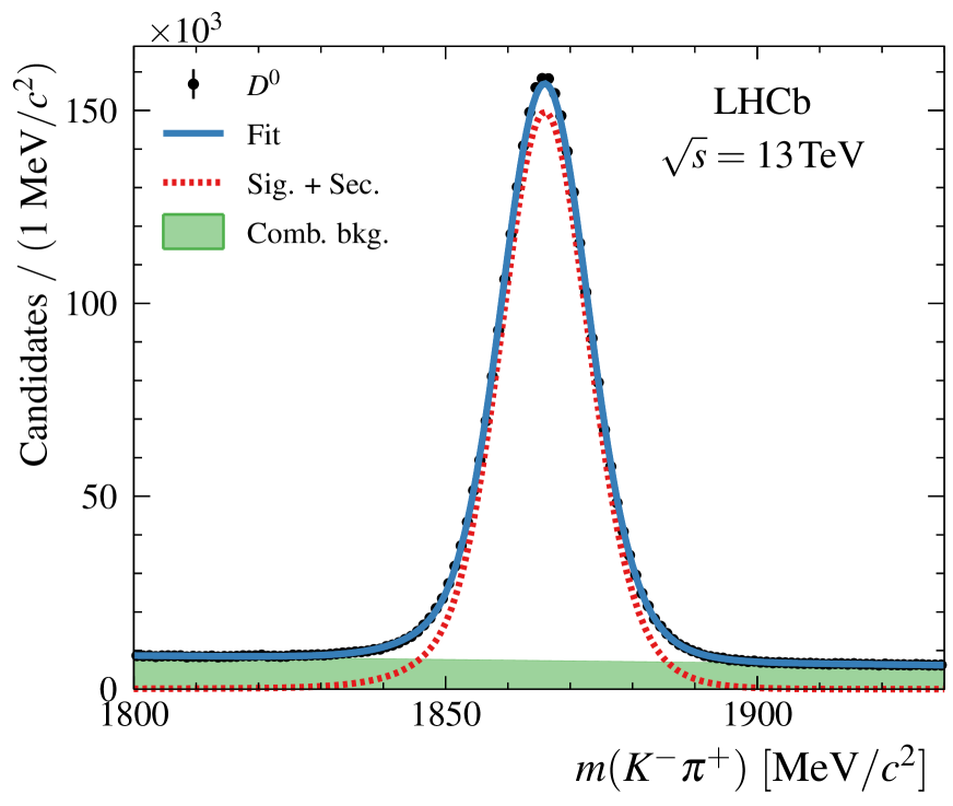
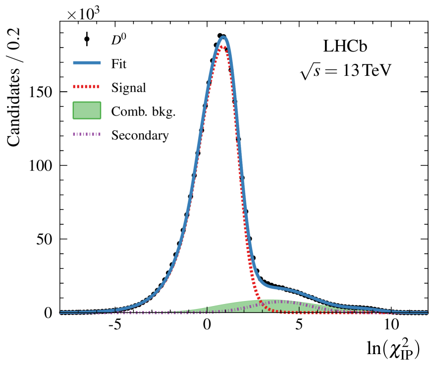
Figure 1: Distributions for selected $D^{0}\to K^{-}\pi^{+}$ candidates: (left) $K^{-}\pi^{+}$ invariant mass and (right) $\ln{\chi^{2}_{\rm IP}}$ for a mass window of $\pm$20\text{\,}\mathrm{{\mathrm{\,Me\kern-0.90005ptV\!/}c^{2}}}$$ around the nominal $D^{0}$ mass. The sum of the simultaneous likelihood fits in each $(p_{\mathrm{T}},y)$ bin is shown, with components as indicated in the legends.

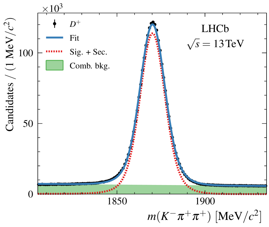
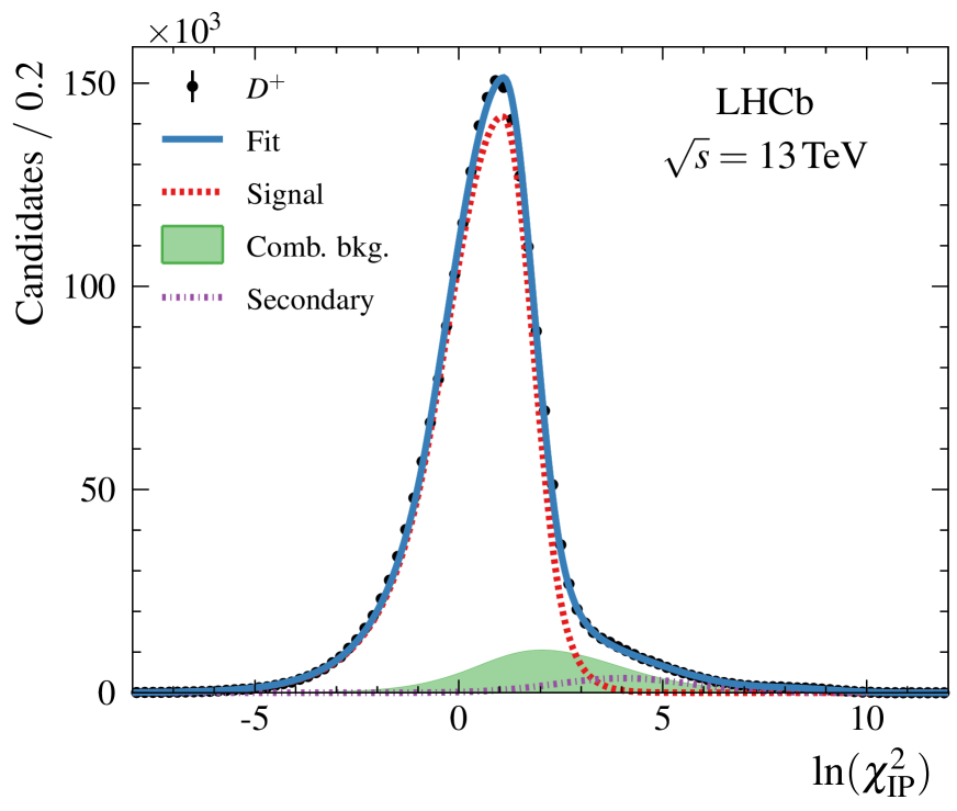
Figure 2: Distributions for selected $D^{+}\to K^{-}\pi^{+}\pi^{+}$ candidates: (left) $K^{-}\pi^{+}\pi^{+}$ invariant mass and (right) $\ln{\chi^{2}_{\rm IP}}$ for a mass window of $\pm$20\text{\,}\mathrm{{\mathrm{\,Me\kern-0.90005ptV\!/}c^{2}}}$$ around the nominal $D^{+}$ mass. The sum of the simultaneous likelihood fits in each $(p_{\mathrm{T}},y)$ bin is shown, with components as indicated in the legends.

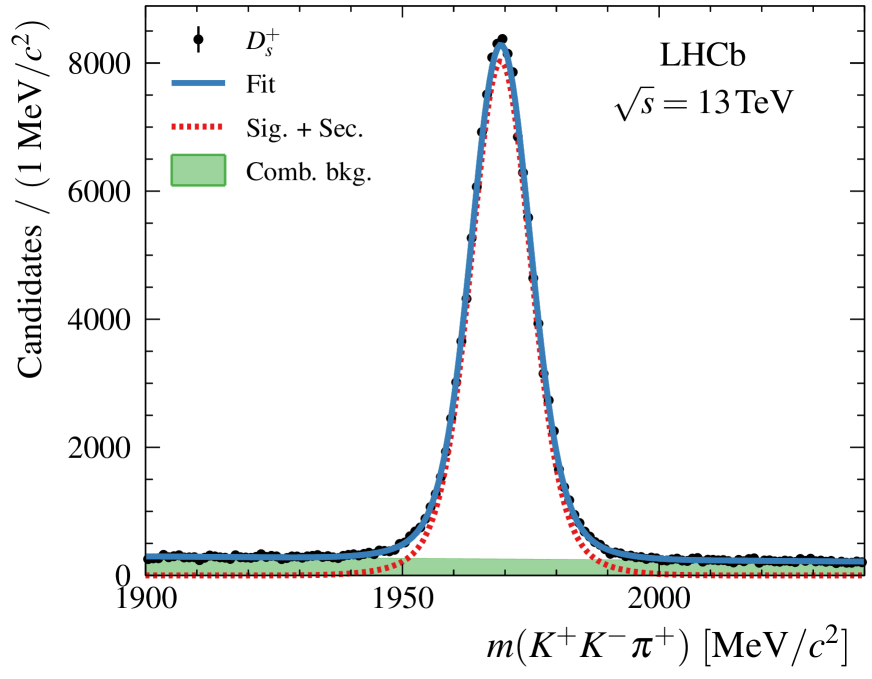
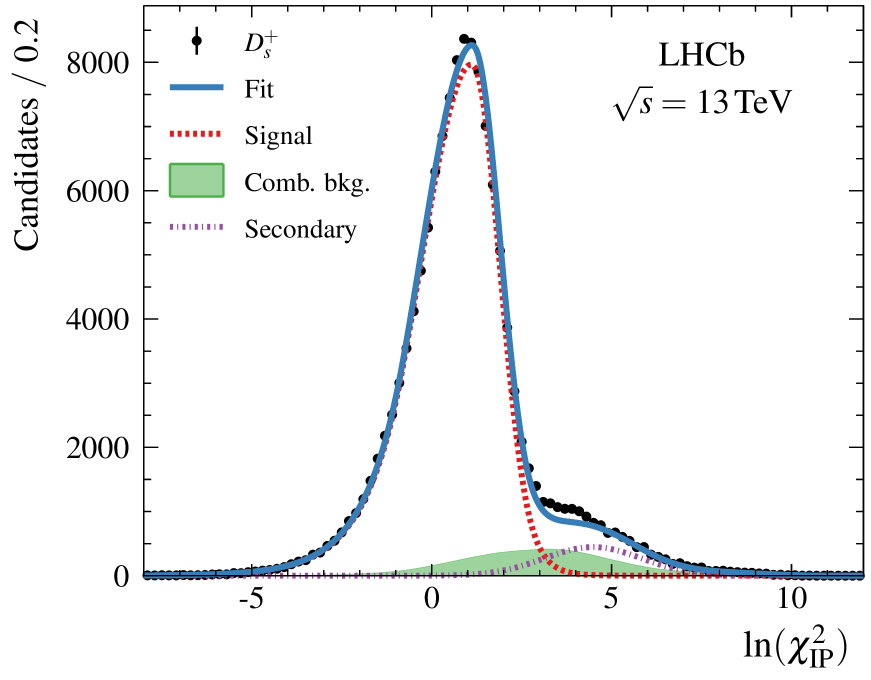
Figure 3: Distributions for selected $D_{s}^{+}\to(K^{-}K^{+})_{\phi}\pi^{+}$ candidates: (left) $K^{+}K^{-}\pi^{+}$ invariant mass and (right) $\ln{\chi^{2}_{\rm IP}}$ for a mass window of $\pm$20\text{\,}\mathrm{{\mathrm{\,Me\kern-0.90005ptV\!/}c^{2}}}$$ around the nominal $D_{s}^{+}$ mass. The sum of the simultaneous likelihood fits in each $(p_{\mathrm{T}},y)$ bin is shown, with components as indicated in the legends.

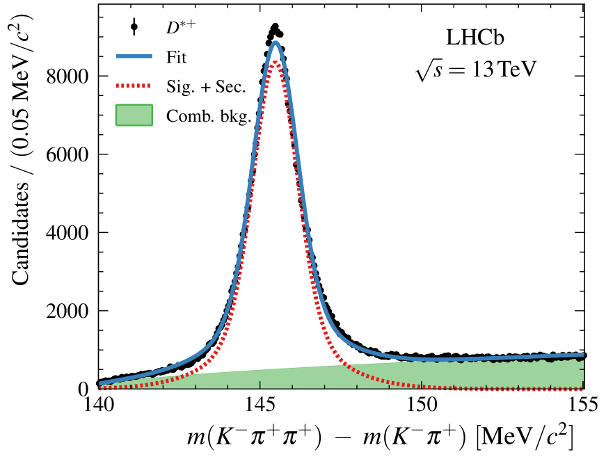
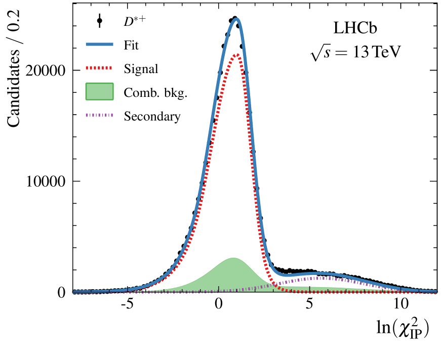
Figure 4: Distributions for selected $D^{*+}\to D^{0}\pi^{+}$ candidates, with $D^{0}\to K^{-}\pi^{+}$: (left) $\Delta{m}=m(D^{*+})-m(D^{0})$ for a mass window of $\pm$20\text{\,}\mathrm{{\mathrm{\,Me\kern-0.90005ptV\!/}c^{2}}}$$ around the nominal $D^{0}$ mass and (right) $\ln{\chi^{2}_{\rm IP}}$ with an additional mass window of $\pm$3\text{\,}\mathrm{{\mathrm{\,Me\kern-0.90005ptV\!/}c^{2}}}$$ around the nominal $D^{*+}$- $D^{0}$ mass difference. The sum of the simultaneous likelihood fits in each $(p_{\mathrm{T}},y)$ bin is shown, with components as indicated in the legends.

Table 1: Prompt signal yields in the fully selected dataset, summed over all ($p_{\mathrm{T}}$,$y$) bins in which a measurement is made.

Hadron	Prompt signal yield
$D^{0}$	$(25.77\pm 0.02)\times 10^{5}$
$D^{+}$	$(19.74\pm 0.02)\times 10^{5}$
$D_{s}^{+}$	$(11.32\pm 0.04)\times 10^{4}$
$D^{*+}$	$(30.12\pm 0.06)\times 10^{4}$

4 Cross-section measurements

The signal yields are used to measure differential cross-sections in bins of $p_{\mathrm{T}}$ and $y$ in the range $0<p_{\mathrm{T}}<15$ $\mathrm{{\mathrm{\,Ge\kern-1.00006ptV\!/}c}}$ and $2.0<y<4.5$. The differential cross-section for producing the charm meson species $D$ in bin $i$ is calculated from the relation

$$\frac{\text{d}^{2}\sigma_{i}(D)}{\text{d}p_{\mathrm{T}}\,\text{d}y}=\frac{1}{\Delta p_{\mathrm{T}}\Delta y}\cdot\frac{N_{i}(\mbox{$D\to f$}+\text{c.c.})}{\varepsilon_{i,\text{tot}}(\mbox{$D\to f$})\mathcal{B}(\mbox{$D\to f$})\kappa\mathcal{L}_{\text{int}}},$$ (3)

where $\Delta p_{\mathrm{T}}$ and $\Delta y$ are the widths in $p_{\mathrm{T}}$ and $y$ of bin $i$, $N_{i}(\mbox{$D\to f$}+\text{c.c.})$ is the measured yield of prompt $D$ decays to the final state $f$ in bin $i$ plus the charge-conjugate decay, $\mathcal{B}(\mbox{$D\to f$})$ is the known branching fraction of the decay, and $\varepsilon_{i,\text{tot}}(\mbox{$D\to f$})$ is the total efficiency for observing the signal decay in bin $i$. The total integrated luminosity collected $\mathcal{L}_{\text{int}}$ is $4.98\pm 0.19\text{\,}{\mathrm{pb}}^{-1}$ and $\kappa=10.7\%$ is the average fraction of events passed by the prescaled hardware trigger. The integrated luminosity of the dataset is evaluated with a precision of $3.8\%$ from the number of visible $pp$ collisions and a constant of proportionality that is measured in a dedicated calibration dataset. The absolute luminosity for the calibration dataset is determined from the beam currents, which are measured by LHC instruments, and the beam profiles and overlap integral, which are measured with a beam-gas imaging method [36].

The following branching fractions taken from Ref. [34] are used: $\mathcal{B}(\mbox{$D^{+}\to K^{-}\pi^{+}\pi^{+}$})=(9.13\pm 0.19)\%$, $\mathcal{B}(\mbox{$D^{*+}\to D^{0}(\to K^{-}\pi^{+})\pi^{+}$})=(2.63\pm 0.04)\%$, and $\mathcal{B}(\mbox{$D^{0}\to K^{\mp}\pi^{\pm}$})=(3.89\pm 0.05)\%$. The last is the sum of Cabibbo-favoured and doubly Cabibbo-suppressed branching fractions, which agrees to better than 1% with the HFAG result that accounts for the effects of final-state radiation [37]. For the $D_{s}^{+}$ measurement the fraction of $D_{s}^{+}\to K^{-}K^{+}\pi^{+}$ decays with a $K^{-}K^{+}$ invariant mass in the range $1000<m_{K^{-}K^{+}}<$1040\text{\,}\mathrm{{\mathrm{\,Me\kern-1.00006ptV\!/}c^{2}}}$$ is taken as $(2.24\pm 0.13)\%$ [38].

The measured differential cross-sections are tabulated in Appendix A. These results agree with the absolute cross-sections measured using the cross-check modes that are listed in Section 3. Figures 5 and 6 show the $D^{0}$, $D^{+}$, $D_{s}^{+}$, and $D^{*+}$ cross-section measurements and predictions. The systematic uncertainties are discussed in Sec. 5 and the theory contributions are provided in Refs. [1, 2, 3] and described in Sec. 7.

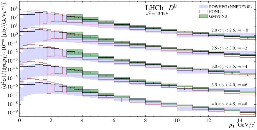
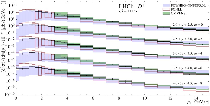
Figure 5: Measurements and predictions for the absolute prompt (top) $D^{0}$, and (bottom) $D^{+}$ cross-sections at $\sqrt{s}=$13\text{\,}\mathrm{TeV}$$. Each set of measurements and predictions in a given rapidity bin is offset by a multiplicative factor $10^{-m}$, where the factor $m$ is shown on the plots. The boxes indicate the $\pm 1\sigma$ uncertainty band on the theory predictions. In cases where this band spans more than two orders of magnitude only its upper edge is indicated.

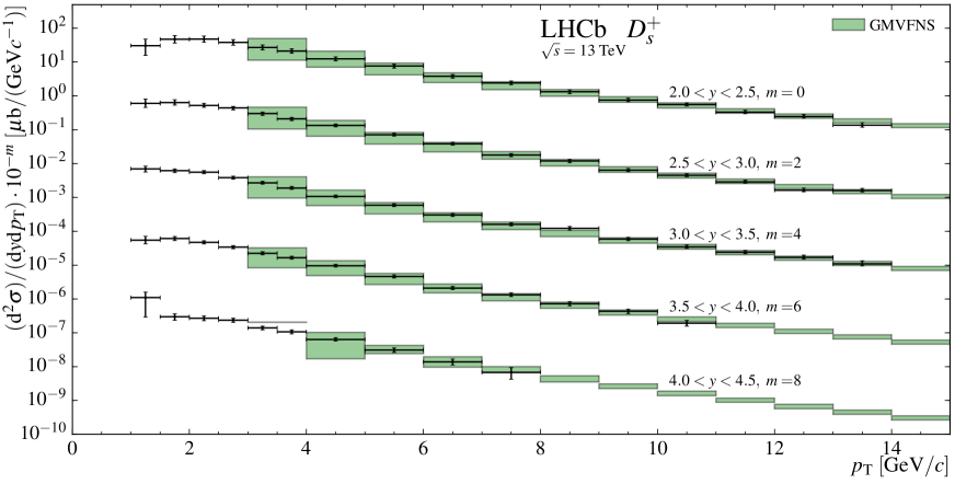
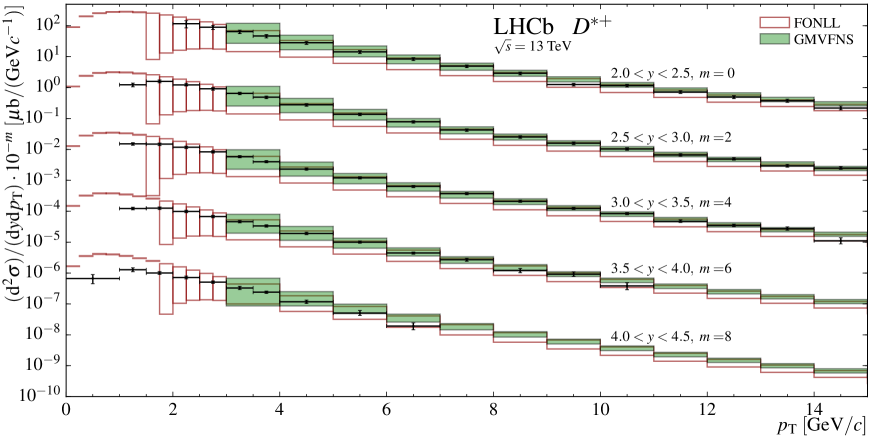
Figure 6: Measurements and predictions for the absolute prompt (top) $D_{s}^{+}$, and (bottom) $D^{*+}$ cross-sections at $\sqrt{s}=$13\text{\,}\mathrm{TeV}$$. Each set of measurements and predictions in a given rapidity bin is offset by a multiplicative factor $10^{-m}$, where the factor $m$ is shown on the plots. The boxes indicate the $\pm 1\sigma$ uncertainty band on the theory predictions. In cases where this band spans more than two orders of magnitude only its upper edge is indicated.

5 Systematic uncertainties

Several sources of systematic uncertainty are identified and evaluated separately for each decay mode and $(p_{\mathrm{T}},y)$ bin. In all cases, the dominant systematic uncertainties originate from the luminosity and the estimation of the tracking efficiencies, amounting to 3.9% and 5–10%, respectively. Uncertainties in the branching fractions give rise to systematic uncertainties between 1% and 5%, depending on the decay mode. Systematic uncertainties are also evaluated to account for the modelling in the simulation, the PID calibration procedure, and the PDF shapes used in the determination of the signal yields. These sum in quadrature to around 5%. Table 2 lists the fractional systematic uncertainties for the different decay modes. Also given are the correlations of each uncertainty between different $(p_{\mathrm{T}},y)$ bins and between different decay modes. The systematic uncertainties can be grouped into three categories: those highly correlated between different decay modes and $(p_{\mathrm{T}},y)$ bins, those that are only correlated between different bins but independent between decay modes, and those that are independent between different decay modes and bins.

The systematic uncertainty on the luminosity is identical for all $(p_{\mathrm{T}},y)$ bins and decay modes. The uncertainty on the tracking efficiency correction is a strongly correlated contribution. It includes a per-track uncertainty on the correction factor that originates from the finite size of the calibration sample, a 0.4% uncertainty stemming from the weighting in different event multiplicity variables, and an additional 1.1% (1.4%) uncertainty for kaon (pion) tracks, due to uncertainties on the amount of material in the detector. The per-track uncertainties are propagated to obtain uncertainties on the correction factor in each $(p_{\mathrm{T}},y)$ bin of the charm meson, and are included as systematic uncertainties, resulting in a 5–10% uncertainty on the measured cross-sections, depending on the decay mode.

The finite sizes of the simulated samples limit the statistical precision of the estimated efficiencies, leading to a systematic uncertainty on the measured cross-sections. As different simulated samples are used for each decay mode, the resulting uncertainty is independent between different decay modes and $(p_{\mathrm{T}},y)$ bins.

Imperfect modelling of variables used in the selection can lead to differences between data and simulation, giving rise to a biased estimate of selection efficiencies. The effect is estimated by comparing the efficiencies when using modified selection criteria. The simulated sample is used to define a tighter requirement for each variable used in the selection, such that 50% of the simulated events are accepted. The same requirement is then applied to the collision data sample, and the signal yield in this subset of the data is compared to the 50% reduction expected from simulation. The procedure is performed separately for each variable used in the selection. The sum of the individual differences, taking the correlations between the variables into account, is assigned as an uncertainty on the signal yield. The corresponding uncertainty on the measured cross-sections is evaluated with Eq. 3.

The systematic uncertainties associated with the PID calibration procedure result from the finite size of the calibration sample and binning effects of the weighting procedure. The PID efficiency in this calibration sample is determined in bins of track momentum, track pseudorapidity, and detector occupancy. The statistical uncertainties of these efficiencies are propagated to obtain systematic uncertainties on the cross-sections. In the weighting procedure, it is assumed that the PID efficiencies for all candidates in a given bin are identical. A systematic uncertainty is assigned to account for deviations from this approximation by sampling from kernel density estimates [39] created from the calibration samples, and recomputing the total PID efficiency with the sampled data using a progressively finer binning. The efficiency converges to a value that is offset from the value measured with the nominal binning. This deviation is assigned as a systematic uncertainty on the PID efficiency. As all decay modes and $(p_{\mathrm{T}},y)$ bins use the same calibration data, this systematic uncertainty is highly correlated between different modes and bins.

Lastly, the systematic uncertainty on the signal yield extracted from the fits is dominated by the uncertainties on the choice of fit model. This is evaluated by refitting the data with different sets of PDFs that are also compatible with the data, and assigning a systematic uncertainty based on the largest deviation in the prompt signal yield.

Table 2: Systematic uncertainties expressed as fractions of the cross-section measurements, in percent. Uncertainties that are computed bin-by-bin are expressed as ranges giving the minimum to maximum values. Ranges for the correlations between $p_{\mathrm{T}}$-$y$ bins and between modes are also given, expressed in percent.

	Uncertainties (%)				Correlations (%)
	$D^{0}$	$D^{+}$	$D_{s}^{+}$	$D^{*+}$	Bins	Modes
Luminosity	3.9				100	100
Tracking	3–10	4–14	4–14	5–11	90–100	90–100
Branching fractions	1.2	2.1	5.8	1.5	100	0–95
Simulation sample size	1–26	1–39	1–55	1–23	0	0
Simulation modelling	1	1	0.2	0.9	0	0
PID sample size	0–2	0–1	0–2	0–1	0–100	0–100
PID binning	0–44	0–10	0–20	0-15	100	100
PDF shapes	1–6	1–5	1–2	1–2	-	-

6 Production ratios and integrated cross-sections

6.1 Production ratios

The predicted ratios of prompt charm production cross-sections between different centre-of-mass energies are devoid of several theoretical uncertainties [1, 2, 3] that are inherent in the corresponding absolute cross-sections. Using the present results obtained at $\sqrt{s}=$13\text{\,}\mathrm{TeV}$$ and the corresponding results from LHCb data at $\sqrt{s}=$7\text{\,}\mathrm{TeV}$$ [16], these ratios, $R_{13/7}$, are measured for $D^{0}$, $D^{+}$, $D_{s}^{+}$, and $D^{*+}$ mesons. The $\sqrt{s}=$13\text{\,}\mathrm{TeV}$$ measurements are rebinned to match the binning used in the $\sqrt{s}=$7\text{\,}\mathrm{TeV}$$ results and the production ratios are presented for $0<p_{\mathrm{T}}<$8\text{\,}\mathrm{{\mathrm{\,Ge\kern-1.00006ptV\!/}c}}$$ and $2.0<y<4.5$ in Appendix B. In the calculation of the uncertainties the branching fraction uncertainties cancel, and correlations of $30\%$ and $50\%$ are assumed for the uncertainties of luminosity and tracking, respectively. All other uncertainties are assumed to be uncorrelated. Figure 7 shows the measured ratios compared with predictions from theory calculations [1, 2, 3].

6.2 Integrated cross-sections

Integrated production cross-sections, $\sigma(D)$, for each charm meson are computed as the sum of the per-bin measurements, where the uncertainty on the sum takes into account the correlations between bins discussed in Section 5. For $D_{s}^{+}$ and $D^{*+}$ mesons, the kinematic region considered is $1<p_{\mathrm{T}}<$8\text{\,}\mathrm{{\mathrm{\,Ge\kern-1.00006ptV\!/}c}}$$ and $2.0<y<4.5$ due to insufficient data below $p_{\mathrm{T}}=$1\text{\,}\mathrm{{\mathrm{\,Ge\kern-1.00006ptV\!/}c}}$$, while for $D^{0}$ and $D^{+}$ the same kinematic region as for the ratio measurements is used. The upper limit is chosen to coincide with that of the measurements at $\sqrt{s}=$7\text{\,}\mathrm{TeV}$$.

The $D^{0}$ and $D^{*+}$ cross-section results contain bins in which a measurement was not possible and which require a correction that is based on theory calculations. A multiplicative correction factor is computed as the ratio between the predicted integrated cross-section within the considered kinematic region and the sum of all per-bin cross-section predictions for bins for which a measurement exists. This method is based on the POWHEG+NNPDF3.0L predictions [1] for $D^{0}$ and the FONLL predictions [2] for $D^{*+}$. The uncertainty on the extrapolation factor is taken as the difference between factors computed using the upper and lower bounds of the theory predictions and is propagated to the integrated cross-sections as a systematic uncertainty. Table 3 gives the integrated cross-sections for $D^{0}$, $D^{+}$, $D_{s}^{+}$, and $D^{*+}$ mesons.

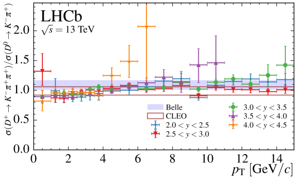
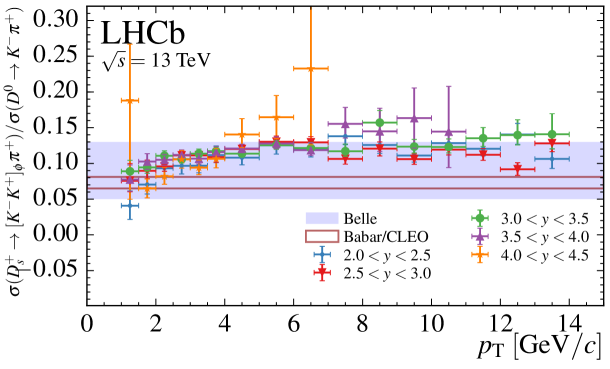
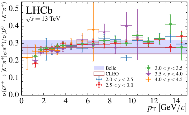
Figure 8: Ratios of cross-section-times-branching-fraction measurements of (top) $D^{+}$, (middle) $D_{s}^{+}$, and (bottom) $D^{*+}$ mesons with respect to the $D^{0}$ measurements. The bands indicate the corresponding ratios computed using measurements from $e^{+}e^{-}$ collider experiments [40, 41, 42]. The ratios are given as a function of $p_{\mathrm{T}}$ and different symbols indicate different ranges in $y$. The notation $\sigma(\mbox{$D\to f$})$ is shorthand for $\sigma(D)\times\mathcal{B}(\mbox{$D\to f$})$.

The ratios of the cross-sections, with the $D^{0}$ and $D^{+}$ results re-evaluated in the kinematic region of the $D_{s}^{+}$ and $D^{*+}$ measurements, can be compared with the ratios of the cross-sections measured at $e^{+}e^{-}$ colliders operating at a centre-of-mass energy close to the $\Upsilon(4S)$ resonance [40, 41, 42]. A more precise comparison is made here by computing the ratios of cross-section-times-branching-fractions, $\sigma(D)\times\mathcal{B}(\mbox{$D\to f$})$, where the final states $f$ are the same between the LHCb measurements and those made at $e^{+}e^{-}$ experiments. Differential ratios are shown in Fig. 8 and tabulated results and remaining figures are presented in Appendix C. They exhibit a $p_{\mathrm{T}}$ dependence that is consistent with heavier particles having a harder $p_{\mathrm{T}}$ spectrum.

The integrated charm cross-section, $\sigma(\mbox{$pp\to c\overline{}cX$})$, is calculated as $\sigma(D)/(2f(\mbox{$c\to D$}))$ for each decay mode. The term $f(\mbox{$c\to D$})$ is the quark to hadron transition probability, and the factor 2 accounts for the inclusion of charge conjugate states in the measurement. The transition probabilities have been computed using measurements at $e^{+}e^{-}$ colliders operating at a centre-of-mass energy close to the $\Upsilon(4S)$ resonance [43] to be $f(\mbox{$c\to D^{0}$})=0.565\pm 0.032$, $f(\mbox{$c\to D^{+}$})=0.246\pm 0.020$, $f(\mbox{$c\to D_{s}^{+}$})=0.080\pm 0.017$, and $f(\mbox{$c\to D^{*+}$})=0.224\pm 0.028$. The fragmentation fraction $f(\mbox{$c\to D^{0}$})$ has an overlapping contribution from $f(\mbox{$c\to D^{*+}$})$.

The combination of the $D^{0}$ and $D^{+}$ measurements, based on the Blue method [44], gives

$$\sigma(\mbox{$pp\to c\overline{}cX$})_{p_{\mathrm{T}}\,<\,8\,$\mathrm{{\mathrm{\,Ge\kern-0.70004ptV\!/}c}}$,\,2.0\,<\,y\,<\,4.5}=$2369\pm 3\pm 152\pm 118\text{\,}\mathrm{\SIUnitSymbolMicro b}$,$$

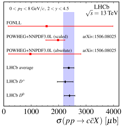
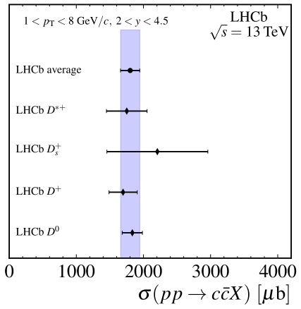
Figure 9: Integrated cross-sections (black diamonds), their average (black circle and blue band) and theory predictions (red squares) [1, 2] are shown (left) based on the $D^{0}$ and $D^{+}$ for $0<p_{\mathrm{T}}<$8\text{\,}\mathrm{{\mathrm{\,Ge\kern-0.90005ptV\!/}c}}$$ and (right) for measurements based on all four mesons for $1<p_{\mathrm{T}}<$8\text{\,}\mathrm{{\mathrm{\,Ge\kern-0.90005ptV\!/}c}}$$. The “absolute” predictions are based on calculations of the $13\text{\,}\mathrm{TeV}$ cross-section, while the “scaled” predictions are based on calculations of the $13$ to $7\text{\,}\mathrm{TeV}$ ratio multiplied with the LHCb measurement at $7\text{\,}\mathrm{TeV}$ [16].

where the uncertainties are due to statistical, systematic and fragmentation fraction uncertainties, respectively. A comparison with predictions is given in Fig. 9. The same figure also shows a comparison of $\sigma(\mbox{$pp\to c\overline{}cX$})$ for $1<p_{\mathrm{T}}<$8\text{\,}\mathrm{{\mathrm{\,Ge\kern-1.00006ptV\!/}c}}$$ based on the measurements of all four mesons. Ratios of the integrated cross-section-time-branching-fraction measurements are given in Table 4.

Table 3: Prompt charm production cross-sections in the kinematic ranges given. The computation of the extrapolation factors is described in the text. The first uncertainty on the cross-section is statistical, and the second is systematic and includes the contribution from the extrapolation factor. No extrapolation factor is given for $D^{+}_{(s)}$ as a measurement is available in every bin of the integrated phase space.

Extrapolation factor Cross-section ($\mathrm{\SIUnitSymbolMicro b}$) $D^{0}$ $0<p_{\mathrm{T}}<$8\text{\,}\mathrm{\giga\kern-1.99997pt\per\kern-1.49994pt}$$ $2<y<4.5$ $1.0014\pm 0.0024$ $2709\pm\phantom{1}2\pm 165$ $D^{+}$ $0<p_{\mathrm{T}}<$8\text{\,}\mathrm{\giga\kern-1.99997pt\per\kern-1.49994pt}$$ $2<y<4.5$ $1.049\pm 0.031$ $1102\pm\phantom{1}5\pm 111$ $D^{0}$ $1<p_{\mathrm{T}}<$8\text{\,}\mathrm{\giga\kern-1.99997pt\per\kern-1.49994pt}$$ $2<y<4.5$ $1.0018\pm 0.0025$ $2072\pm\phantom{1}2\pm 124$ $D^{+}$ $1<p_{\mathrm{T}}<$8\text{\,}\mathrm{\giga\kern-1.99997pt\per\kern-1.49994pt}$$ $2<y<4.5$ — $834\pm\phantom{1}2\pm\phantom{1}78$ $D_{s}^{+}$ $1<p_{\mathrm{T}}<$8\text{\,}\mathrm{\giga\kern-1.99997pt\per\kern-1.49994pt}$$ $2<y<4.5$ — $353\pm\phantom{1}9\pm\phantom{1}76$ $D^{*+}$ $1<p_{\mathrm{T}}<$8\text{\,}\mathrm{\giga\kern-1.99997pt\per\kern-1.49994pt}$$ $2<y<4.5$ $1.102\pm 0.081$ $784\pm\phantom{1}4\pm\phantom{1}87$ $D^{0}$ $0<p_{\mathrm{T}}<$8\text{\,}\mathrm{\giga\kern-1.99997pt\per\kern-1.49994pt}$$ $2.5<y<4$ — $1720\pm\phantom{1}1\pm\phantom{1}98$ $D^{+}$ $0<p_{\mathrm{T}}<$8\text{\,}\mathrm{\giga\kern-1.99997pt\per\kern-1.49994pt}$$ $2.5<y<4$ — $706\pm\phantom{1}4\pm\phantom{1}66$ $D^{0}$ $1<p_{\mathrm{T}}<$8\text{\,}\mathrm{\giga\kern-1.99997pt\per\kern-1.49994pt}$$ $2.5<y<4$ — $1313\pm\phantom{1}1\pm\phantom{1}73$ $D^{+}$ $1<p_{\mathrm{T}}<$8\text{\,}\mathrm{\giga\kern-1.99997pt\per\kern-1.49994pt}$$ $2.5<y<4$ — $527\pm\phantom{1}1\pm\phantom{1}45$ $D_{s}^{+}$ $1<p_{\mathrm{T}}<$8\text{\,}\mathrm{\giga\kern-1.99997pt\per\kern-1.49994pt}$$ $2.5<y<4$ — $227\pm\phantom{1}2\pm\phantom{1}24$ $D^{*+}$ $1<p_{\mathrm{T}}<$8\text{\,}\mathrm{\giga\kern-1.99997pt\per\kern-1.49994pt}$$ $2.5<y<4$ — $493\pm\phantom{1}2\pm\phantom{1}41$

Table 4: Ratios of integrated cross-section-times-branching-fraction measurements in the kinematic range $1<p_{\mathrm{T}}<$8\text{\,}\mathrm{{\mathrm{\,Ge\kern-0.90005ptV\!/}c}}$$ and $2<y<4.5$. The first uncertainty on the ratio is statistical and the second is systematic. The notation $\sigma(\mbox{$D\to f$})$ is shorthand for $\sigma(D)\times\mathcal{B}(\mbox{$D\to f$})$.

Quantity Measurement $\sigma(\mbox{$D^{+}\to K^{-}\pi^{+}\pi^{+}$})/\sigma(\mbox{$D^{0}\to K^{-}\pi^{+}$})$ $\phantom{1}0.950^{+\phantom{1}0.003}_{-\phantom{1}0.003}$${}^{+\phantom{1}0.040}_{-\phantom{1}0.040}$ $\sigma(D_{s}^{+}\to[K^{-}K^{+}]_{\phi}\pi^{+})/\sigma(\mbox{$D^{0}\to K^{-}\pi^{+}$})$ $0.0991^{+0.0026}_{-0.0026}$${}^{+0.0053}_{-0.0079}$ $\sigma(D^{*+}\to[K^{-}\pi^{+}]_{D^{0}}\pi^{+})/\sigma(\mbox{$D^{0}\to K^{-}\pi^{+}$})$ $\phantom{1}0.256^{+\phantom{1}0.001}_{-\phantom{1}0.001}$${}^{+\phantom{1}0.021}_{-\phantom{1}0.021}$ $\sigma(D_{s}^{+}\to[K^{-}K^{+}]_{\phi}\pi^{+})/\sigma(\mbox{$D^{+}\to K^{-}\pi^{+}\pi^{+}$})$ $0.1043^{+0.0028}_{-0.0028}$${}^{+0.0038}_{-0.0066}$ $\sigma(D^{*+}\to[K^{-}\pi^{+}]_{D^{0}}\pi^{+})/\sigma(\mbox{$D^{+}\to K^{-}\pi^{+}\pi^{+}$})$ $\phantom{1}0.270^{+\phantom{1}0.002}_{-\phantom{1}0.002}$${}^{+\phantom{1}0.023}_{-\phantom{1}0.022}$ $\sigma(D_{s}^{+}\to[K^{-}K^{+}]_{\phi}\pi^{+})/\sigma(D^{*+}\to[K^{-}\pi^{+}]_{D^{0}}\pi^{+})$ $\phantom{1}0.390^{+\phantom{1}0.010}_{-\phantom{1}0.010}$${}^{+\phantom{1}0.038}_{-\phantom{1}0.045}$

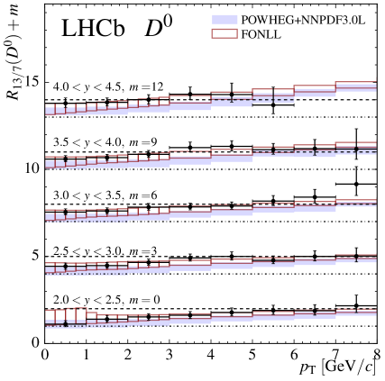
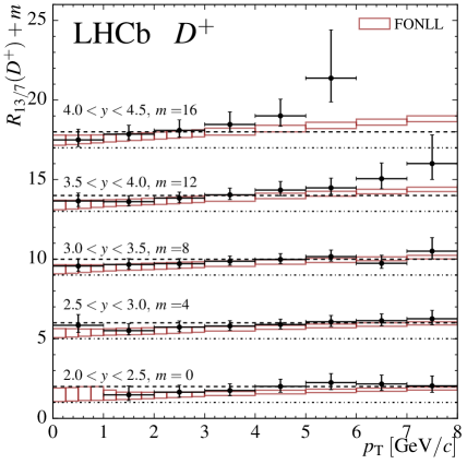
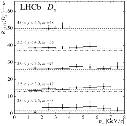
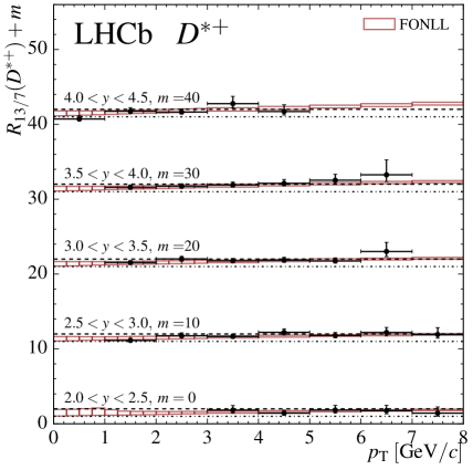
Figure 7: Measurements and predictions of the prompt $D^{0}$, $D^{+}$, $D_{s}^{+}$, and $D^{*+}$ cross-section ratios. The dash-dotted lines indicate the unit ratio for each of the rapidity intervals and the dashed lines indicate a ratio of two. Each set of measurements and predictions in a given rapidity bin is offset by an additive constant $m$, which is shown on the plot. No prediction is available for the $D_{s}^{+}$ ratio.

7 Comparison to theory

Theoretical calculations for charm meson production cross-sections in $pp$ collisions at $\sqrt{s}=$13\text{\,}\mathrm{TeV}$$ have been provided in Refs. [1] (POWHEG+NNPDF3.0L), [2] (FONLL), and [3] (GMVFNS). All three sets of calculations are performed at NLO precision, and each includes estimates of theoretical uncertainties due to the renormalisation and factorisation scales. The theoretical uncertainties provided with the FONLL and POWHEG+NNPDF3.0L predictions also include contributions due to uncertainties in the effective charm quark mass and the parton distribution functions.

The FONLL predictions are provided in the form of $D^{0}$, $D^{+}$, and $D^{*+}$ production cross-sections for $pp$ collisions at $\sqrt{s}=$13\text{\,}\mathrm{TeV}$$ for each bin in a subdivision of the phase space, $p_{\mathrm{T}}<$30\text{\,}\mathrm{{\mathrm{\,Ge\kern-1.00006ptV\!/}c}}$$ and $2.0<y<4.5$. Ratios of these cross-sections to those computed for $pp$ collisions at $7\text{\,}\mathrm{TeV}$ are also supplied. The calculations use the NNPDF3.0 NLO [45] parton densities. These FONLL calculations of the meson differential production cross-sections assume $f(\mbox{$c\to D$})=1$ and are multiplied by the transition probabilities measured at $e^{+}e^{-}$ colliders for comparison to the current measurements. No dedicated FONLL cross-section calculation for $D_{s}^{+}$ production is available.

The POWHEG+NNPDF3.0L predictions are also provided in the form of $D^{0}$ and $D^{+}$ production cross-sections for $pp$ collisions at $\sqrt{s}=$13\text{\,}\mathrm{TeV}$$ for each bin in a subdivision of the phase space, $p_{\mathrm{T}}<$30\text{\,}\mathrm{{\mathrm{\,Ge\kern-1.00006ptV\!/}c}}$$ and $2.0<y<4.5$. Ratios of $13$ to $7\text{\,}\mathrm{TeV}$ cross-sections are given as well. They are obtained with Powheg [46] matched to Pythia8 [47] parton showers and an improved version of the NNPDF3.0 NLO parton distribution function set designated NNPDF3.0+LHCb [1]. To produce this improved set, the authors of Ref. [1] weight the NNPDF3.0 NLO set in order to match FONLL calculations to LHCb’s charm cross-section measurements at $7\text{\,}\mathrm{TeV}$ [16]. This results in a significant improvement in the uncertainties for the gluon distribution function at small momentum fraction $x$. Two predictions for the integrated cross-section are provided, one an absolute calculation, identical to that for the differential cross-sections, and the other scaled from the $7\text{\,}\mathrm{TeV}$ measurement.

The GMVFNS calculations include theoretical predictions for all mesons studied in this analysis. Results are provided for $3<p_{\mathrm{T}}<$30\text{\,}\mathrm{{\mathrm{\,Ge\kern-1.00006ptV\!/}c}}$$. Here the CT10 [48] set of parton distributions is used. The GMVFNS theoretical framework includes the convolution with fragmentation functions describing the transition $c\to H_{c}$ that are normalised to the respective total transition probabilities [7, 49]. The fragmentation functions are taken from a fit to production measurements at $e^{+}e^{-}$ colliders, where no attempt is made to separate direct production and feed-down from higher resonances.

In general, the data shown in Figures 5 and 6 agree with the predicted shapes of the cross-sections at $\sqrt{s}=$13\text{\,}\mathrm{TeV}$$ for all three sets of calculations. The central values of the measurements generally lie above those of the POWHEG+NNPDF3.0L and FONLL predictions, albeit within the uncertainties provided. The GMVFNS predictions provide the best description of the data, although the cross-section measurements decrease with $p_{\mathrm{T}}$ at a higher rate than the predictions. Similar behaviour is observed for the $\sqrt{s}=$7\text{\,}\mathrm{TeV}$$ measurement [16], where only central values are shown for the FONLL prediction which give lower cross-sections than the data.

The predictions are in agreement with the data for the ratios of cross-sections at $\sqrt{s}=$13\text{\,}\mathrm{TeV}$$ and $7\text{\,}\mathrm{TeV}$, shown in Figure 7, though consistently at the upper limit of the predicted values.

The absolute predictions for the integrated cross-sections show agreement with data within their large uncertainties, with central values below the measurements. The scaled POWHEG+NNPDF3.0L prediction, which has smaller uncertainties than the absolute prediction, agrees with the data. The measurements are consistent with a linear scaling of the cross-section with the collision energy.

8 Summary

A measurement of charm production in $pp$ collisions at a centre-of-mass energy of $\sqrt{s}=$13\text{\,}\mathrm{TeV}$$ has been performed with data collected with the LHCb detector. The shapes of the differential cross-sections for $D^{0}$, $D^{+}$, $D^{*+}$, and $D_{s}^{+}$ mesons are found to be in agreement with NLO predictions while the predicted central values generally lie below the data, albeit mostly within uncertainties. The ratios of the production cross-sections for centre-of-mass energies of $13\text{\,}\mathrm{T}\mathrm{e}\mathrm{V}$ and $7\text{\,}\mathrm{T}\mathrm{e}\mathrm{V}$ have been measured and also show consistency with theoretical predictions. The $c\overline{}c$ cross-section for production of a charm meson in $pp$ collisions at $\sqrt{s}=$13\text{\,}\mathrm{T}\mathrm{e}\mathrm{V}$$ and in the range $0<p_{\mathrm{T}}<$8\text{\,}\mathrm{{\mathrm{\,Ge\kern-1.00006ptV\!/}c}}$$ and $2<y<4.5$ is $2369\pm 3\pm 152\pm 118\text{\,}\mathrm{\SIUnitSymbolMicro b}$.

Appendix A Absolute cross-sections

Tables A–A give the numerical results for the differential cross-sections.

Table 5: Differential production cross-sections, $\text{d}^{2}\sigma/(\text{d}p_{\mathrm{T}}\,\text{d}y)$, in $$\mathrm{\SIUnitSymbolMicro b}$/($\mathrm{{\mathrm{\,Ge\kern-0.90005ptV\!/}c}}$)$ for prompt $D^{0}+{\kern 1.79997pt\overline{\kern-1.79997ptD}{}}^{0}$ mesons in bins of $(p_{\mathrm{T}},y)$. The first uncertainty is statistical, and the second is the total systematic.    $y$ $p_{\text{T}}$ [MeV/c] $[2,2.5]$ $[2.5,3]$ $[3,3.5]$ $[3.5,4]$ $[4,4.5]$ $[0,1000]$ $254$ ${}^{+}_{-}$ ${}^{2}_{2}$ ${}^{+}_{-}$ ${}^{31}_{27}$ $277.3$ ${}^{+}_{-}$ ${}^{1.0}_{1.0}$ ${}^{+}_{-}$ ${}^{21.4}_{24.8}$ $281.1$ ${}^{+}_{-}$ ${}^{0.9}_{0.9}$ ${}^{+}_{-}$ ${}^{19.4}_{17.4}$ $256$ ${}^{+}_{-}$ ${}^{1}_{1}$ ${}^{+}_{-}$ ${}^{16}_{14}$ $206$ ${}^{+}_{-}$ ${}^{2}_{2}$ ${}^{+}_{-}$ ${}^{16}_{14}$ $[1000,1500]$ $433$ ${}^{+}_{-}$ ${}^{3}_{3}$ ${}^{+}_{-}$ ${}^{50}_{45}$ $457$ ${}^{+}_{-}$ ${}^{2}_{2}$ ${}^{+}_{-}$ ${}^{32}_{37}$ $454$ ${}^{+}_{-}$ ${}^{1}_{1}$ ${}^{+}_{-}$ ${}^{28}_{27}$ $409$ ${}^{+}_{-}$ ${}^{2}_{2}$ ${}^{+}_{-}$ ${}^{25}_{23}$ $337$ ${}^{+}_{-}$ ${}^{3}_{3}$ ${}^{+}_{-}$ ${}^{25}_{22}$ $[1500,2000]$ $388$ ${}^{+}_{-}$ ${}^{2}_{2}$ ${}^{+}_{-}$ ${}^{40}_{37}$ $409$ ${}^{+}_{-}$ ${}^{1}_{1}$ ${}^{+}_{-}$ ${}^{30}_{26}$ $380$ ${}^{+}_{-}$ ${}^{1}_{1}$ ${}^{+}_{-}$ ${}^{23}_{22}$ $344$ ${}^{+}_{-}$ ${}^{1}_{1}$ ${}^{+}_{-}$ ${}^{21}_{19}$ $265$ ${}^{+}_{-}$ ${}^{2}_{2}$ ${}^{+}_{-}$ ${}^{18}_{17}$ $[2000,2500]$ $296$ ${}^{+}_{-}$ ${}^{2}_{2}$ ${}^{+}_{-}$ ${}^{24}_{28}$ $314.4$ ${}^{+}_{-}$ ${}^{1.0}_{1.0}$ ${}^{+}_{-}$ ${}^{21.1}_{18.7}$ $292.5$ ${}^{+}_{-}$ ${}^{0.9}_{0.9}$ ${}^{+}_{-}$ ${}^{17.4}_{15.8}$ $259$ ${}^{+}_{-}$ ${}^{1}_{1}$ ${}^{+}_{-}$ ${}^{16}_{14}$ $190$ ${}^{+}_{-}$ ${}^{2}_{2}$ ${}^{+}_{-}$ ${}^{11}_{12}$ $[2500,3000]$ $228$ ${}^{+}_{-}$ ${}^{1}_{1}$ ${}^{+}_{-}$ ${}^{17}_{20}$ $228.9$ ${}^{+}_{-}$ ${}^{0.7}_{0.7}$ ${}^{+}_{-}$ ${}^{14.7}_{13.2}$ $208.8$ ${}^{+}_{-}$ ${}^{0.7}_{0.7}$ ${}^{+}_{-}$ ${}^{12.6}_{10.4}$ $175.0$ ${}^{+}_{-}$ ${}^{0.8}_{0.8}$ ${}^{+}_{-}$ ${}^{11.3}_{\phantom{0}9.5}$ $129.6$ ${}^{+}_{-}$ ${}^{1.2}_{1.2}$ ${}^{+}_{-}$ ${}^{8.3}_{8.9}$ $[3000,3500]$ $161.3$ ${}^{+}_{-}$ ${}^{0.9}_{0.9}$ ${}^{+}_{-}$ ${}^{11.4}_{13.0}$ $156.1$ ${}^{+}_{-}$ ${}^{0.5}_{0.5}$ ${}^{+}_{-}$ ${}^{9.6}_{8.7}$ $137.3$ ${}^{+}_{-}$ ${}^{0.5}_{0.5}$ ${}^{+}_{-}$ ${}^{8.1}_{6.9}$ $121.4$ ${}^{+}_{-}$ ${}^{0.6}_{0.6}$ ${}^{+}_{-}$ ${}^{8.5}_{6.9}$ $85.6$ ${}^{+}_{-}$ ${}^{0.9}_{0.9}$ ${}^{+}_{-}$ ${}^{6.3}_{6.4}$ $[3500,4000]$ $109.7$ ${}^{+}_{-}$ ${}^{0.6}_{0.6}$ ${}^{+}_{-}$ ${}^{7.3}_{8.2}$ $111.0$ ${}^{+}_{-}$ ${}^{0.4}_{0.4}$ ${}^{+}_{-}$ ${}^{6.6}_{6.0}$ $93.5$ ${}^{+}_{-}$ ${}^{0.4}_{0.4}$ ${}^{+}_{-}$ ${}^{5.5}_{4.7}$ $82.7$ ${}^{+}_{-}$ ${}^{0.4}_{0.4}$ ${}^{+}_{-}$ ${}^{5.5}_{4.9}$ $58.0$ ${}^{+}_{-}$ ${}^{0.8}_{0.8}$ ${}^{+}_{-}$ ${}^{5.9}_{5.5}$ $[4000,5000]$ $66.5$ ${}^{+}_{-}$ ${}^{0.3}_{0.3}$ ${}^{+}_{-}$ ${}^{4.7}_{4.2}$ $64.5$ ${}^{+}_{-}$ ${}^{0.2}_{0.2}$ ${}^{+}_{-}$ ${}^{3.9}_{3.3}$ $54.5$ ${}^{+}_{-}$ ${}^{0.2}_{0.2}$ ${}^{+}_{-}$ ${}^{3.2}_{2.7}$ $45.9$ ${}^{+}_{-}$ ${}^{0.2}_{0.2}$ ${}^{+}_{-}$ ${}^{2.5}_{2.7}$ $26.1$ ${}^{+}_{-}$ ${}^{0.4}_{0.4}$ ${}^{+}_{-}$ ${}^{3.6}_{3.0}$ $[5000,6000]$ $35.5$ ${}^{+}_{-}$ ${}^{0.2}_{0.2}$ ${}^{+}_{-}$ ${}^{2.6}_{2.1}$ $31.5$ ${}^{+}_{-}$ ${}^{0.1}_{0.1}$ ${}^{+}_{-}$ ${}^{1.8}_{1.6}$ $27.1$ ${}^{+}_{-}$ ${}^{0.1}_{0.1}$ ${}^{+}_{-}$ ${}^{1.5}_{1.6}$ $20.8$ ${}^{+}_{-}$ ${}^{0.1}_{0.1}$ ${}^{+}_{-}$ ${}^{1.3}_{1.2}$ $10.9$ ${}^{+}_{-}$ ${}^{0.4}_{0.4}$ ${}^{+}_{-}$ ${}^{2.5}_{1.8}$ $[6000,7000]$ $18.5$ ${}^{+}_{-}$ ${}^{0.1}_{0.1}$ ${}^{+}_{-}$ ${}^{1.3}_{1.2}$ $17.20$ ${}^{+}_{-}$ ${}^{0.09}_{0.09}$ ${}^{+}_{-}$ ${}^{0.96}_{0.92}$ $14.40$ ${}^{+}_{-}$ ${}^{0.09}_{0.09}$ ${}^{+}_{-}$ ${}^{0.82}_{0.85}$ $10.20$ ${}^{+}_{-}$ ${}^{0.12}_{0.12}$ ${}^{+}_{-}$ ${}^{0.87}_{0.81}$ $3.4$ ${}^{+}_{-}$ ${}^{0.5}_{0.5}$ ${}^{+}_{-}$ ${}^{2.4}_{1.3}$ $[7000,8000]$ $10.15$ ${}^{+}_{-}$ ${}^{0.09}_{0.09}$ ${}^{+}_{-}$ ${}^{0.72}_{0.63}$ $9.71$ ${}^{+}_{-}$ ${}^{0.07}_{0.07}$ ${}^{+}_{-}$ ${}^{0.60}_{0.52}$ $7.88$ ${}^{+}_{-}$ ${}^{0.07}_{0.07}$ ${}^{+}_{-}$ ${}^{0.42}_{0.48}$ $4.94$ ${}^{+}_{-}$ ${}^{0.10}_{0.10}$ ${}^{+}_{-}$ ${}^{0.71}_{0.58}$ $[8000,9000]$ $6.11$ ${}^{+}_{-}$ ${}^{0.07}_{0.07}$ ${}^{+}_{-}$ ${}^{0.46}_{0.39}$ $5.72$ ${}^{+}_{-}$ ${}^{0.05}_{0.05}$ ${}^{+}_{-}$ ${}^{0.38}_{0.32}$ $4.49$ ${}^{+}_{-}$ ${}^{0.05}_{0.05}$ ${}^{+}_{-}$ ${}^{0.27}_{0.29}$ $2.88$ ${}^{+}_{-}$ ${}^{0.11}_{0.11}$ ${}^{+}_{-}$ ${}^{0.57}_{0.44}$ $[9000,10000]$ $3.92$ ${}^{+}_{-}$ ${}^{0.06}_{0.06}$ ${}^{+}_{-}$ ${}^{0.26}_{0.22}$ $3.48$ ${}^{+}_{-}$ ${}^{0.04}_{0.04}$ ${}^{+}_{-}$ ${}^{0.21}_{0.15}$ $2.75$ ${}^{+}_{-}$ ${}^{0.04}_{0.04}$ ${}^{+}_{-}$ ${}^{0.16}_{0.13}$ $1.53$ ${}^{+}_{-}$ ${}^{0.11}_{0.11}$ ${}^{+}_{-}$ ${}^{0.49}_{0.28}$ $[10000,11000]$ $2.48$ ${}^{+}_{-}$ ${}^{0.05}_{0.05}$ ${}^{+}_{-}$ ${}^{0.18}_{0.16}$ $2.18$ ${}^{+}_{-}$ ${}^{0.03}_{0.03}$ ${}^{+}_{-}$ ${}^{0.14}_{0.09}$ $1.62$ ${}^{+}_{-}$ ${}^{0.04}_{0.04}$ ${}^{+}_{-}$ ${}^{0.12}_{0.09}$ $0.77$ ${}^{+}_{-}$ ${}^{0.13}_{0.13}$ ${}^{+}_{-}$ ${}^{0.33}_{0.16}$ $[11000,12000]$ $1.59$ ${}^{+}_{-}$ ${}^{0.04}_{0.04}$ ${}^{+}_{-}$ ${}^{0.14}_{0.10}$ $1.49$ ${}^{+}_{-}$ ${}^{0.03}_{0.03}$ ${}^{+}_{-}$ ${}^{0.10}_{0.06}$ $1.025$ ${}^{+}_{-}$ ${}^{0.034}_{0.034}$ ${}^{+}_{-}$ ${}^{0.083}_{0.056}$ $[12000,13000]$ $1.01$ ${}^{+}_{-}$ ${}^{0.03}_{0.03}$ ${}^{+}_{-}$ ${}^{0.12}_{0.08}$ $1.031$ ${}^{+}_{-}$ ${}^{0.026}_{0.026}$ ${}^{+}_{-}$ ${}^{0.078}_{0.037}$ $0.716$ ${}^{+}_{-}$ ${}^{0.034}_{0.034}$ ${}^{+}_{-}$ ${}^{0.060}_{0.048}$ $[13000,14000]$ $0.746$ ${}^{+}_{-}$ ${}^{0.026}_{0.026}$ ${}^{+}_{-}$ ${}^{0.089}_{0.055}$ $0.718$ ${}^{+}_{-}$ ${}^{0.023}_{0.023}$ ${}^{+}_{-}$ ${}^{0.060}_{0.025}$ $0.447$ ${}^{+}_{-}$ ${}^{0.031}_{0.031}$ ${}^{+}_{-}$ ${}^{0.075}_{0.045}$ $[14000,15000]$ $0.498$ ${}^{+}_{-}$ ${}^{0.022}_{0.022}$ ${}^{+}_{-}$ ${}^{0.058}_{0.030}$ $0.495$ ${}^{+}_{-}$ ${}^{0.020}_{0.020}$ ${}^{+}_{-}$ ${}^{0.048}_{0.022}$ $0.268$ ${}^{+}_{-}$ ${}^{0.031}_{0.031}$ ${}^{+}_{-}$ ${}^{0.053}_{0.031}$

Table 6: Differential production cross-sections, $\text{d}^{2}\sigma/(\text{d}p_{\mathrm{T}}\,\text{d}y)$, in $$\mathrm{\SIUnitSymbolMicro b}$/($\mathrm{{\mathrm{\,Ge\kern-0.90005ptV\!/}c}}$)$ for prompt $D^{+}+D^{-}$ mesons in bins of $(p_{\mathrm{T}},y)$. The first uncertainty is statistical, and the second is the total systematic.    $y$ $p_{\text{T}}$ [MeV/c] $[2,2.5]$ $[2.5,3]$ $[3,3.5]$ $[3.5,4]$ $[4,4.5]$ $[0,1000]$ $156$ ${}^{+}_{-}$ ${}^{6}_{6}$ ${}^{+}_{-}$ ${}^{38}_{32}$ $107$ ${}^{+}_{-}$ ${}^{3}_{3}$ ${}^{+}_{-}$ ${}^{15}_{14}$ $97$ ${}^{+}_{-}$ ${}^{3}_{3}$ ${}^{+}_{-}$ ${}^{13}_{13}$ $72$ ${}^{+}_{-}$ ${}^{5}_{5}$ ${}^{+}_{-}$ ${}^{16}_{14}$ $[1000,1500]$ $182$ ${}^{+}_{-}$ ${}^{7}_{7}$ ${}^{+}_{-}$ ${}^{47}_{42}$ $170$ ${}^{+}_{-}$ ${}^{2}_{2}$ ${}^{+}_{-}$ ${}^{31}_{22}$ $184$ ${}^{+}_{-}$ ${}^{1}_{1}$ ${}^{+}_{-}$ ${}^{19}_{18}$ $158$ ${}^{+}_{-}$ ${}^{2}_{2}$ ${}^{+}_{-}$ ${}^{15}_{14}$ $137$ ${}^{+}_{-}$ ${}^{3}_{3}$ ${}^{+}_{-}$ ${}^{16}_{15}$ $[1500,2000]$ $146$ ${}^{+}_{-}$ ${}^{2}_{2}$ ${}^{+}_{-}$ ${}^{27}_{23}$ $149.5$ ${}^{+}_{-}$ ${}^{0.8}_{0.8}$ ${}^{+}_{-}$ ${}^{23.0}_{16.6}$ $153.5$ ${}^{+}_{-}$ ${}^{0.7}_{0.7}$ ${}^{+}_{-}$ ${}^{13.7}_{14.2}$ $133.6$ ${}^{+}_{-}$ ${}^{0.7}_{0.7}$ ${}^{+}_{-}$ ${}^{11.4}_{10.4}$ $107.1$ ${}^{+}_{-}$ ${}^{1.2}_{1.2}$ ${}^{+}_{-}$ ${}^{9.6}_{9.1}$ $[2000,2500]$ $111$ ${}^{+}_{-}$ ${}^{1}_{1}$ ${}^{+}_{-}$ ${}^{18}_{16}$ $126.1$ ${}^{+}_{-}$ ${}^{0.5}_{0.5}$ ${}^{+}_{-}$ ${}^{16.4}_{12.9}$ $115.4$ ${}^{+}_{-}$ ${}^{0.4}_{0.4}$ ${}^{+}_{-}$ ${}^{9.5}_{9.7}$ $97.4$ ${}^{+}_{-}$ ${}^{0.4}_{0.4}$ ${}^{+}_{-}$ ${}^{7.8}_{7.2}$ $78.9$ ${}^{+}_{-}$ ${}^{0.7}_{0.7}$ ${}^{+}_{-}$ ${}^{6.3}_{6.1}$ $[2500,3000]$ $86.1$ ${}^{+}_{-}$ ${}^{0.7}_{0.7}$ ${}^{+}_{-}$ ${}^{13.1}_{12.3}$ $94.0$ ${}^{+}_{-}$ ${}^{0.3}_{0.3}$ ${}^{+}_{-}$ ${}^{\phantom{0}8.8}_{10.0}$ $83.5$ ${}^{+}_{-}$ ${}^{0.3}_{0.3}$ ${}^{+}_{-}$ ${}^{6.5}_{6.5}$ $72.1$ ${}^{+}_{-}$ ${}^{0.3}_{0.3}$ ${}^{+}_{-}$ ${}^{5.4}_{5.1}$ $53.2$ ${}^{+}_{-}$ ${}^{0.4}_{0.4}$ ${}^{+}_{-}$ ${}^{4.4}_{4.0}$ $[3000,3500]$ $62.3$ ${}^{+}_{-}$ ${}^{0.5}_{0.5}$ ${}^{+}_{-}$ ${}^{8.8}_{8.6}$ $66.7$ ${}^{+}_{-}$ ${}^{0.2}_{0.2}$ ${}^{+}_{-}$ ${}^{6.0}_{6.6}$ $59.3$ ${}^{+}_{-}$ ${}^{0.2}_{0.2}$ ${}^{+}_{-}$ ${}^{4.6}_{4.3}$ $49.7$ ${}^{+}_{-}$ ${}^{0.2}_{0.2}$ ${}^{+}_{-}$ ${}^{3.8}_{3.4}$ $35.0$ ${}^{+}_{-}$ ${}^{0.3}_{0.3}$ ${}^{+}_{-}$ ${}^{2.7}_{2.7}$ $[3500,4000]$ $42.4$ ${}^{+}_{-}$ ${}^{0.3}_{0.3}$ ${}^{+}_{-}$ ${}^{5.5}_{5.6}$ $46.4$ ${}^{+}_{-}$ ${}^{0.2}_{0.2}$ ${}^{+}_{-}$ ${}^{4.2}_{4.2}$ $42.0$ ${}^{+}_{-}$ ${}^{0.2}_{0.2}$ ${}^{+}_{-}$ ${}^{3.3}_{2.9}$ $33.3$ ${}^{+}_{-}$ ${}^{0.2}_{0.2}$ ${}^{+}_{-}$ ${}^{2.7}_{2.2}$ $22.6$ ${}^{+}_{-}$ ${}^{0.2}_{0.2}$ ${}^{+}_{-}$ ${}^{1.7}_{1.8}$ $[4000,5000]$ $29.2$ ${}^{+}_{-}$ ${}^{0.2}_{0.2}$ ${}^{+}_{-}$ ${}^{3.2}_{3.7}$ $28.22$ ${}^{+}_{-}$ ${}^{0.09}_{0.09}$ ${}^{+}_{-}$ ${}^{2.35}_{2.34}$ $23.36$ ${}^{+}_{-}$ ${}^{0.08}_{0.08}$ ${}^{+}_{-}$ ${}^{1.83}_{1.48}$ $19.29$ ${}^{+}_{-}$ ${}^{0.08}_{0.08}$ ${}^{+}_{-}$ ${}^{1.51}_{1.26}$ $13.9$ ${}^{+}_{-}$ ${}^{0.1}_{0.1}$ ${}^{+}_{-}$ ${}^{0.9}_{1.1}$ $[5000,6000]$ $15.1$ ${}^{+}_{-}$ ${}^{0.1}_{0.1}$ ${}^{+}_{-}$ ${}^{1.5}_{1.7}$ $14.49$ ${}^{+}_{-}$ ${}^{0.06}_{0.06}$ ${}^{+}_{-}$ ${}^{1.18}_{1.10}$ $12.18$ ${}^{+}_{-}$ ${}^{0.05}_{0.05}$ ${}^{+}_{-}$ ${}^{0.94}_{0.78}$ $9.44$ ${}^{+}_{-}$ ${}^{0.05}_{0.05}$ ${}^{+}_{-}$ ${}^{0.71}_{0.63}$ $6.87$ ${}^{+}_{-}$ ${}^{0.11}_{0.11}$ ${}^{+}_{-}$ ${}^{0.60}_{0.64}$ $[6000,7000]$ $8.34$ ${}^{+}_{-}$ ${}^{0.07}_{0.07}$ ${}^{+}_{-}$ ${}^{0.76}_{0.84}$ $7.39$ ${}^{+}_{-}$ ${}^{0.04}_{0.04}$ ${}^{+}_{-}$ ${}^{0.59}_{0.54}$ $6.30$ ${}^{+}_{-}$ ${}^{0.04}_{0.04}$ ${}^{+}_{-}$ ${}^{0.49}_{0.40}$ $4.89$ ${}^{+}_{-}$ ${}^{0.04}_{0.04}$ ${}^{+}_{-}$ ${}^{0.32}_{0.37}$ $3.03$ ${}^{+}_{-}$ ${}^{0.09}_{0.09}$ ${}^{+}_{-}$ ${}^{0.32}_{0.30}$ $[7000,8000]$ $4.98$ ${}^{+}_{-}$ ${}^{0.05}_{0.05}$ ${}^{+}_{-}$ ${}^{0.47}_{0.46}$ $4.24$ ${}^{+}_{-}$ ${}^{0.03}_{0.03}$ ${}^{+}_{-}$ ${}^{0.33}_{0.31}$ $3.51$ ${}^{+}_{-}$ ${}^{0.03}_{0.03}$ ${}^{+}_{-}$ ${}^{0.28}_{0.23}$ $2.56$ ${}^{+}_{-}$ ${}^{0.03}_{0.03}$ ${}^{+}_{-}$ ${}^{0.18}_{0.21}$ $2.31$ ${}^{+}_{-}$ ${}^{0.13}_{0.13}$ ${}^{+}_{-}$ ${}^{0.53}_{0.47}$ $[8000,9000]$ $3.11$ ${}^{+}_{-}$ ${}^{0.04}_{0.04}$ ${}^{+}_{-}$ ${}^{0.31}_{0.25}$ $2.63$ ${}^{+}_{-}$ ${}^{0.02}_{0.02}$ ${}^{+}_{-}$ ${}^{0.21}_{0.19}$ $2.16$ ${}^{+}_{-}$ ${}^{0.02}_{0.02}$ ${}^{+}_{-}$ ${}^{0.17}_{0.14}$ $1.40$ ${}^{+}_{-}$ ${}^{0.02}_{0.02}$ ${}^{+}_{-}$ ${}^{0.12}_{0.13}$ $1.17$ ${}^{+}_{-}$ ${}^{0.09}_{0.09}$ ${}^{+}_{-}$ ${}^{0.46}_{0.47}$ $[9000,10000]$ $1.46$ ${}^{+}_{-}$ ${}^{0.02}_{0.02}$ ${}^{+}_{-}$ ${}^{0.13}_{0.11}$ $1.35$ ${}^{+}_{-}$ ${}^{0.01}_{0.01}$ ${}^{+}_{-}$ ${}^{0.11}_{0.09}$ $1.192$ ${}^{+}_{-}$ ${}^{0.015}_{0.015}$ ${}^{+}_{-}$ ${}^{0.083}_{0.083}$ $0.928$ ${}^{+}_{-}$ ${}^{0.025}_{0.025}$ ${}^{+}_{-}$ ${}^{0.096}_{0.087}$ $[10000,11000]$ $1.144$ ${}^{+}_{-}$ ${}^{0.020}_{0.020}$ ${}^{+}_{-}$ ${}^{0.098}_{0.081}$ $0.970$ ${}^{+}_{-}$ ${}^{0.013}_{0.013}$ ${}^{+}_{-}$ ${}^{0.072}_{0.061}$ $0.784$ ${}^{+}_{-}$ ${}^{0.013}_{0.013}$ ${}^{+}_{-}$ ${}^{0.050}_{0.052}$ $0.477$ ${}^{+}_{-}$ ${}^{0.020}_{0.020}$ ${}^{+}_{-}$ ${}^{0.057}_{0.044}$ $[11000,12000]$ $0.774$ ${}^{+}_{-}$ ${}^{0.016}_{0.016}$ ${}^{+}_{-}$ ${}^{0.070}_{0.054}$ $0.641$ ${}^{+}_{-}$ ${}^{0.011}_{0.011}$ ${}^{+}_{-}$ ${}^{0.050}_{0.037}$ $0.520$ ${}^{+}_{-}$ ${}^{0.011}_{0.011}$ ${}^{+}_{-}$ ${}^{0.035}_{0.034}$ $0.301$ ${}^{+}_{-}$ ${}^{0.017}_{0.017}$ ${}^{+}_{-}$ ${}^{0.031}_{0.021}$ $[12000,13000]$ $0.513$ ${}^{+}_{-}$ ${}^{0.012}_{0.012}$ ${}^{+}_{-}$ ${}^{0.049}_{0.033}$ $0.443$ ${}^{+}_{-}$ ${}^{0.009}_{0.009}$ ${}^{+}_{-}$ ${}^{0.036}_{0.025}$ $0.336$ ${}^{+}_{-}$ ${}^{0.009}_{0.009}$ ${}^{+}_{-}$ ${}^{0.024}_{0.021}$ $0.185$ ${}^{+}_{-}$ ${}^{0.011}_{0.011}$ ${}^{+}_{-}$ ${}^{0.034}_{0.021}$ $[13000,14000]$ $0.362$ ${}^{+}_{-}$ ${}^{0.010}_{0.010}$ ${}^{+}_{-}$ ${}^{0.037}_{0.023}$ $0.298$ ${}^{+}_{-}$ ${}^{0.007}_{0.007}$ ${}^{+}_{-}$ ${}^{0.028}_{0.015}$ $0.238$ ${}^{+}_{-}$ ${}^{0.008}_{0.008}$ ${}^{+}_{-}$ ${}^{0.019}_{0.014}$ $0.096$ ${}^{+}_{-}$ ${}^{0.009}_{0.009}$ ${}^{+}_{-}$ ${}^{0.015}_{0.006}$ $[14000,15000]$ $0.250$ ${}^{+}_{-}$ ${}^{0.008}_{0.008}$ ${}^{+}_{-}$ ${}^{0.028}_{0.014}$ $0.212$ ${}^{+}_{-}$ ${}^{0.006}_{0.006}$ ${}^{+}_{-}$ ${}^{0.022}_{0.009}$ $0.162$ ${}^{+}_{-}$ ${}^{0.007}_{0.007}$ ${}^{+}_{-}$ ${}^{0.017}_{0.007}$

Table 7: Differential production cross-sections, $\text{d}^{2}\sigma/(\text{d}p_{\mathrm{T}}\,\text{d}y)$, in $$\mathrm{\SIUnitSymbolMicro b}$/($\mathrm{{\mathrm{\,Ge\kern-0.90005ptV\!/}c}}$)$ for prompt $D_{s}^{+}+D_{s}^{-}$ mesons in bins of $(p_{\mathrm{T}},y)$. The first uncertainty is statistical, and the second is the total systematic.    $y$ $p_{\text{T}}$ [MeV/c] $[2,2.5]$ $[2.5,3]$ $[3,3.5]$ $[3.5,4]$ $[4,4.5]$ $[1000,1500]$ $31$ ${}^{+}_{-}$ ${}^{8}_{8}$ ${}^{+}_{-}$ ${}^{15}_{13}$ $60$ ${}^{+}_{-}$ ${}^{4}_{4}$ ${}^{+}_{-}$ ${}^{21}_{13}$ $70$ ${}^{+}_{-}$ ${}^{4}_{4}$ ${}^{+}_{-}$ ${}^{13}_{13}$ $55$ ${}^{+}_{-}$ ${}^{5}_{5}$ ${}^{+}_{-}$ ${}^{14}_{11}$ $110$ ${}^{+}_{-}$ ${}^{36}_{36}$ ${}^{+}_{-}$ ${}^{34}_{72}$ $[1500,2000]$ $47$ ${}^{+}_{-}$ ${}^{3}_{3}$ ${}^{+}_{-}$ ${}^{13}_{10}$ $63$ ${}^{+}_{-}$ ${}^{2}_{2}$ ${}^{+}_{-}$ ${}^{14}_{10}$ $62.1$ ${}^{+}_{-}$ ${}^{1.6}_{1.6}$ ${}^{+}_{-}$ ${}^{7.5}_{7.2}$ $61.2$ ${}^{+}_{-}$ ${}^{2.2}_{2.2}$ ${}^{+}_{-}$ ${}^{8.5}_{7.2}$ $29.8$ ${}^{+}_{-}$ ${}^{3.1}_{3.1}$ ${}^{+}_{-}$ ${}^{5.9}_{5.5}$ $[2000,2500]$ $48$ ${}^{+}_{-}$ ${}^{2}_{2}$ ${}^{+}_{-}$ ${}^{11}_{\phantom{0}9}$ $52.2$ ${}^{+}_{-}$ ${}^{0.9}_{0.9}$ ${}^{+}_{-}$ ${}^{8.4}_{5.8}$ $56.1$ ${}^{+}_{-}$ ${}^{0.9}_{0.9}$ ${}^{+}_{-}$ ${}^{6.2}_{5.6}$ $47.1$ ${}^{+}_{-}$ ${}^{1.1}_{1.1}$ ${}^{+}_{-}$ ${}^{5.3}_{4.7}$ $26.9$ ${}^{+}_{-}$ ${}^{1.8}_{1.8}$ ${}^{+}_{-}$ ${}^{4.2}_{3.7}$ $[2500,3000]$ $38.2$ ${}^{+}_{-}$ ${}^{1.1}_{1.1}$ ${}^{+}_{-}$ ${}^{7.8}_{6.5}$ $44.1$ ${}^{+}_{-}$ ${}^{0.6}_{0.6}$ ${}^{+}_{-}$ ${}^{4.9}_{5.5}$ $38.3$ ${}^{+}_{-}$ ${}^{0.5}_{0.5}$ ${}^{+}_{-}$ ${}^{4.2}_{3.3}$ $33.9$ ${}^{+}_{-}$ ${}^{0.7}_{0.7}$ ${}^{+}_{-}$ ${}^{3.5}_{3.2}$ $23.7$ ${}^{+}_{-}$ ${}^{1.1}_{1.1}$ ${}^{+}_{-}$ ${}^{3.2}_{3.1}$ $[3000,3500]$ $27.1$ ${}^{+}_{-}$ ${}^{0.7}_{0.7}$ ${}^{+}_{-}$ ${}^{4.9}_{4.2}$ $30.1$ ${}^{+}_{-}$ ${}^{0.4}_{0.4}$ ${}^{+}_{-}$ ${}^{3.2}_{3.4}$ $27.0$ ${}^{+}_{-}$ ${}^{0.4}_{0.4}$ ${}^{+}_{-}$ ${}^{2.9}_{2.3}$ $22.4$ ${}^{+}_{-}$ ${}^{0.4}_{0.4}$ ${}^{+}_{-}$ ${}^{2.3}_{2.1}$ $13.9$ ${}^{+}_{-}$ ${}^{0.7}_{0.7}$ ${}^{+}_{-}$ ${}^{1.7}_{1.6}$ $[3500,4000]$ $21.2$ ${}^{+}_{-}$ ${}^{0.5}_{0.5}$ ${}^{+}_{-}$ ${}^{3.6}_{3.0}$ $20.9$ ${}^{+}_{-}$ ${}^{0.3}_{0.3}$ ${}^{+}_{-}$ ${}^{2.2}_{2.2}$ $19.0$ ${}^{+}_{-}$ ${}^{0.3}_{0.3}$ ${}^{+}_{-}$ ${}^{2.0}_{1.6}$ $16.6$ ${}^{+}_{-}$ ${}^{0.3}_{0.3}$ ${}^{+}_{-}$ ${}^{1.7}_{1.5}$ $10.7$ ${}^{+}_{-}$ ${}^{0.6}_{0.6}$ ${}^{+}_{-}$ ${}^{1.5}_{1.3}$ $[4000,5000]$ $12.4$ ${}^{+}_{-}$ ${}^{0.2}_{0.2}$ ${}^{+}_{-}$ ${}^{1.8}_{1.6}$ $13.4$ ${}^{+}_{-}$ ${}^{0.2}_{0.2}$ ${}^{+}_{-}$ ${}^{1.4}_{1.3}$ $10.7$ ${}^{+}_{-}$ ${}^{0.1}_{0.1}$ ${}^{+}_{-}$ ${}^{1.1}_{0.9}$ $9.60$ ${}^{+}_{-}$ ${}^{0.17}_{0.17}$ ${}^{+}_{-}$ ${}^{0.93}_{0.87}$ $6.36$ ${}^{+}_{-}$ ${}^{0.28}_{0.28}$ ${}^{+}_{-}$ ${}^{0.78}_{0.61}$ $[5000,6000]$ $7.7$ ${}^{+}_{-}$ ${}^{0.2}_{0.2}$ ${}^{+}_{-}$ ${}^{0.9}_{1.0}$ $7.11$ ${}^{+}_{-}$ ${}^{0.11}_{0.11}$ ${}^{+}_{-}$ ${}^{0.79}_{0.59}$ $5.89$ ${}^{+}_{-}$ ${}^{0.10}_{0.10}$ ${}^{+}_{-}$ ${}^{0.58}_{0.49}$ $4.62$ ${}^{+}_{-}$ ${}^{0.10}_{0.10}$ ${}^{+}_{-}$ ${}^{0.54}_{0.41}$ $3.10$ ${}^{+}_{-}$ ${}^{0.20}_{0.20}$ ${}^{+}_{-}$ ${}^{0.45}_{0.40}$ $[6000,7000]$ $3.83$ ${}^{+}_{-}$ ${}^{0.10}_{0.10}$ ${}^{+}_{-}$ ${}^{0.44}_{0.46}$ $3.85$ ${}^{+}_{-}$ ${}^{0.08}_{0.08}$ ${}^{+}_{-}$ ${}^{0.41}_{0.34}$ $3.03$ ${}^{+}_{-}$ ${}^{0.07}_{0.07}$ ${}^{+}_{-}$ ${}^{0.31}_{0.27}$ $2.10$ ${}^{+}_{-}$ ${}^{0.07}_{0.07}$ ${}^{+}_{-}$ ${}^{0.25}_{0.20}$ $1.39$ ${}^{+}_{-}$ ${}^{0.16}_{0.16}$ ${}^{+}_{-}$ ${}^{0.25}_{0.21}$ $[7000,8000]$ $2.43$ ${}^{+}_{-}$ ${}^{0.08}_{0.08}$ ${}^{+}_{-}$ ${}^{0.32}_{0.26}$ $1.79$ ${}^{+}_{-}$ ${}^{0.05}_{0.05}$ ${}^{+}_{-}$ ${}^{0.18}_{0.17}$ $1.60$ ${}^{+}_{-}$ ${}^{0.05}_{0.05}$ ${}^{+}_{-}$ ${}^{0.18}_{0.14}$ $1.33$ ${}^{+}_{-}$ ${}^{0.06}_{0.06}$ ${}^{+}_{-}$ ${}^{0.18}_{0.14}$ $0.68$ ${}^{+}_{-}$ ${}^{0.18}_{0.18}$ ${}^{+}_{-}$ ${}^{0.18}_{0.18}$ $[8000,9000]$ $1.33$ ${}^{+}_{-}$ ${}^{0.05}_{0.05}$ ${}^{+}_{-}$ ${}^{0.17}_{0.14}$ $1.19$ ${}^{+}_{-}$ ${}^{0.04}_{0.04}$ ${}^{+}_{-}$ ${}^{0.13}_{0.12}$ $1.22$ ${}^{+}_{-}$ ${}^{0.04}_{0.04}$ ${}^{+}_{-}$ ${}^{0.16}_{0.12}$ $0.72$ ${}^{+}_{-}$ ${}^{0.05}_{0.05}$ ${}^{+}_{-}$ ${}^{0.10}_{0.09}$ $[9000,10000]$ $0.754$ ${}^{+}_{-}$ ${}^{0.036}_{0.036}$ ${}^{+}_{-}$ ${}^{0.097}_{0.067}$ $0.639$ ${}^{+}_{-}$ ${}^{0.026}_{0.026}$ ${}^{+}_{-}$ ${}^{0.069}_{0.054}$ $0.588$ ${}^{+}_{-}$ ${}^{0.027}_{0.027}$ ${}^{+}_{-}$ ${}^{0.066}_{0.050}$ $0.433$ ${}^{+}_{-}$ ${}^{0.041}_{0.041}$ ${}^{+}_{-}$ ${}^{0.053}_{0.044}$ $[10000,11000]$ $0.553$ ${}^{+}_{-}$ ${}^{0.032}_{0.032}$ ${}^{+}_{-}$ ${}^{0.063}_{0.037}$ $0.450$ ${}^{+}_{-}$ ${}^{0.023}_{0.023}$ ${}^{+}_{-}$ ${}^{0.045}_{0.031}$ $0.346$ ${}^{+}_{-}$ ${}^{0.022}_{0.022}$ ${}^{+}_{-}$ ${}^{0.043}_{0.023}$ $0.192$ ${}^{+}_{-}$ ${}^{0.033}_{0.033}$ ${}^{+}_{-}$ ${}^{0.025}_{0.010}$ $[11000,12000]$ $0.331$ ${}^{+}_{-}$ ${}^{0.025}_{0.025}$ ${}^{+}_{-}$ ${}^{0.038}_{0.023}$ $0.289$ ${}^{+}_{-}$ ${}^{0.018}_{0.018}$ ${}^{+}_{-}$ ${}^{0.031}_{0.017}$ $0.240$ ${}^{+}_{-}$ ${}^{0.018}_{0.018}$ ${}^{+}_{-}$ ${}^{0.028}_{0.012}$ $[12000,13000]$ $0.247$ ${}^{+}_{-}$ ${}^{0.020}_{0.020}$ ${}^{+}_{-}$ ${}^{0.030}_{0.016}$ $0.164$ ${}^{+}_{-}$ ${}^{0.014}_{0.014}$ ${}^{+}_{-}$ ${}^{0.020}_{0.008}$ $0.169$ ${}^{+}_{-}$ ${}^{0.016}_{0.016}$ ${}^{+}_{-}$ ${}^{0.022}_{0.006}$ $[13000,14000]$ $0.137$ ${}^{+}_{-}$ ${}^{0.016}_{0.016}$ ${}^{+}_{-}$ ${}^{0.019}_{0.009}$ $0.159$ ${}^{+}_{-}$ ${}^{0.014}_{0.014}$ ${}^{+}_{-}$ ${}^{0.022}_{0.006}$ $0.1090$ ${}^{+}_{-}$ ${}^{0.0146}_{0.0146}$ ${}^{+}_{-}$ ${}^{0.0212}_{0.0010}$ $[14000,15000]$

Table 8: Differential production cross-sections, $\text{d}^{2}\sigma/(\text{d}p_{\mathrm{T}}\,\text{d}y)$, in $$\mathrm{\SIUnitSymbolMicro b}$/($\mathrm{{\mathrm{\,Ge\kern-0.90005ptV\!/}c}}$)$ for prompt $D^{*+}+D^{*-}$ mesons in bins of $(p_{\mathrm{T}},y)$. The first uncertainty is statistical, and the second is the total systematic.    $y$ $p_{\text{T}}$ [MeV/c] $[2,2.5]$ $[2.5,3]$ $[3,3.5]$ $[3.5,4]$ $[4,4.5]$ $[0,1000]$ $67$ ${}^{+}_{-}$ ${}^{9}_{9}$ ${}^{+}_{-}$ ${}^{20}_{19}$ $[1000,1500]$ $124$ ${}^{+}_{-}$ ${}^{5}_{5}$ ${}^{+}_{-}$ ${}^{16}_{17}$ $152$ ${}^{+}_{-}$ ${}^{2}_{2}$ ${}^{+}_{-}$ ${}^{13}_{15}$ $123$ ${}^{+}_{-}$ ${}^{2}_{2}$ ${}^{+}_{-}$ ${}^{12}_{12}$ $127$ ${}^{+}_{-}$ ${}^{4}_{4}$ ${}^{+}_{-}$ ${}^{20}_{16}$ $[1500,2000]$ $159$ ${}^{+}_{-}$ ${}^{3}_{3}$ ${}^{+}_{-}$ ${}^{18}_{16}$ $148$ ${}^{+}_{-}$ ${}^{1}_{1}$ ${}^{+}_{-}$ ${}^{12}_{14}$ $125$ ${}^{+}_{-}$ ${}^{1}_{1}$ ${}^{+}_{-}$ ${}^{11}_{12}$ $100$ ${}^{+}_{-}$ ${}^{2}_{2}$ ${}^{+}_{-}$ ${}^{11}_{\phantom{0}9}$ $[2000,2500]$ $117$ ${}^{+}_{-}$ ${}^{11}_{11}$ ${}^{+}_{-}$ ${}^{27}_{29}$ $123$ ${}^{+}_{-}$ ${}^{1}_{1}$ ${}^{+}_{-}$ ${}^{15}_{10}$ $118.2$ ${}^{+}_{-}$ ${}^{0.8}_{0.8}$ ${}^{+}_{-}$ ${}^{\phantom{0}9.4}_{11.1}$ $98.4$ ${}^{+}_{-}$ ${}^{0.8}_{0.8}$ ${}^{+}_{-}$ ${}^{9.2}_{8.2}$ $71.3$ ${}^{+}_{-}$ ${}^{1.3}_{1.3}$ ${}^{+}_{-}$ ${}^{8.1}_{7.1}$ $[2500,3000]$ $90$ ${}^{+}_{-}$ ${}^{3}_{3}$ ${}^{+}_{-}$ ${}^{13}_{14}$ $91.7$ ${}^{+}_{-}$ ${}^{0.8}_{0.8}$ ${}^{+}_{-}$ ${}^{8.3}_{9.3}$ $83.2$ ${}^{+}_{-}$ ${}^{0.5}_{0.5}$ ${}^{+}_{-}$ ${}^{7.6}_{6.7}$ $67.3$ ${}^{+}_{-}$ ${}^{0.6}_{0.6}$ ${}^{+}_{-}$ ${}^{6.3}_{5.6}$ $50.9$ ${}^{+}_{-}$ ${}^{1.0}_{1.0}$ ${}^{+}_{-}$ ${}^{4.4}_{4.8}$ $[3000,3500]$ $64.8$ ${}^{+}_{-}$ ${}^{1.6}_{1.6}$ ${}^{+}_{-}$ ${}^{7.7}_{9.0}$ $65.2$ ${}^{+}_{-}$ ${}^{0.5}_{0.5}$ ${}^{+}_{-}$ ${}^{5.6}_{6.6}$ $57.9$ ${}^{+}_{-}$ ${}^{0.4}_{0.4}$ ${}^{+}_{-}$ ${}^{5.4}_{4.3}$ $45.7$ ${}^{+}_{-}$ ${}^{0.4}_{0.4}$ ${}^{+}_{-}$ ${}^{4.3}_{3.7}$ $32.8$ ${}^{+}_{-}$ ${}^{0.7}_{0.7}$ ${}^{+}_{-}$ ${}^{4.2}_{3.7}$ $[3500,4000]$ $46.8$ ${}^{+}_{-}$ ${}^{1.0}_{1.0}$ ${}^{+}_{-}$ ${}^{5.3}_{6.1}$ $48.9$ ${}^{+}_{-}$ ${}^{0.4}_{0.4}$ ${}^{+}_{-}$ ${}^{4.2}_{4.9}$ $39.9$ ${}^{+}_{-}$ ${}^{0.3}_{0.3}$ ${}^{+}_{-}$ ${}^{3.7}_{2.9}$ $33.2$ ${}^{+}_{-}$ ${}^{0.3}_{0.3}$ ${}^{+}_{-}$ ${}^{3.1}_{2.7}$ $23.9$ ${}^{+}_{-}$ ${}^{0.6}_{0.6}$ ${}^{+}_{-}$ ${}^{2.1}_{2.1}$ $[4000,5000]$ $28.2$ ${}^{+}_{-}$ ${}^{0.4}_{0.4}$ ${}^{+}_{-}$ ${}^{2.8}_{3.3}$ $27.8$ ${}^{+}_{-}$ ${}^{0.2}_{0.2}$ ${}^{+}_{-}$ ${}^{2.3}_{2.7}$ $22.9$ ${}^{+}_{-}$ ${}^{0.1}_{0.1}$ ${}^{+}_{-}$ ${}^{2.0}_{1.6}$ $19.1$ ${}^{+}_{-}$ ${}^{0.2}_{0.2}$ ${}^{+}_{-}$ ${}^{1.8}_{1.6}$ $11.7$ ${}^{+}_{-}$ ${}^{0.3}_{0.3}$ ${}^{+}_{-}$ ${}^{1.5}_{1.3}$ $[5000,6000]$ $14.3$ ${}^{+}_{-}$ ${}^{0.2}_{0.2}$ ${}^{+}_{-}$ ${}^{1.4}_{1.6}$ $13.7$ ${}^{+}_{-}$ ${}^{0.1}_{0.1}$ ${}^{+}_{-}$ ${}^{1.1}_{1.3}$ $11.96$ ${}^{+}_{-}$ ${}^{0.09}_{0.09}$ ${}^{+}_{-}$ ${}^{1.02}_{0.88}$ $9.91$ ${}^{+}_{-}$ ${}^{0.12}_{0.12}$ ${}^{+}_{-}$ ${}^{0.95}_{0.67}$ $5.1$ ${}^{+}_{-}$ ${}^{0.3}_{0.3}$ ${}^{+}_{-}$ ${}^{1.0}_{0.8}$ $[6000,7000]$ $8.45$ ${}^{+}_{-}$ ${}^{0.14}_{0.14}$ ${}^{+}_{-}$ ${}^{0.79}_{0.94}$ $7.83$ ${}^{+}_{-}$ ${}^{0.07}_{0.07}$ ${}^{+}_{-}$ ${}^{0.64}_{0.73}$ $6.33$ ${}^{+}_{-}$ ${}^{0.06}_{0.06}$ ${}^{+}_{-}$ ${}^{0.50}_{0.49}$ $4.44$ ${}^{+}_{-}$ ${}^{0.08}_{0.08}$ ${}^{+}_{-}$ ${}^{0.35}_{0.35}$ $1.93$ ${}^{+}_{-}$ ${}^{0.32}_{0.32}$ ${}^{+}_{-}$ ${}^{0.40}_{0.36}$ $[7000,8000]$ $4.96$ ${}^{+}_{-}$ ${}^{0.09}_{0.09}$ ${}^{+}_{-}$ ${}^{0.46}_{0.54}$ $4.25$ ${}^{+}_{-}$ ${}^{0.05}_{0.05}$ ${}^{+}_{-}$ ${}^{0.37}_{0.41}$ $3.70$ ${}^{+}_{-}$ ${}^{0.05}_{0.05}$ ${}^{+}_{-}$ ${}^{0.32}_{0.27}$ $2.68$ ${}^{+}_{-}$ ${}^{0.07}_{0.07}$ ${}^{+}_{-}$ ${}^{0.30}_{0.27}$ $[8000,9000]$ $2.91$ ${}^{+}_{-}$ ${}^{0.06}_{0.06}$ ${}^{+}_{-}$ ${}^{0.28}_{0.32}$ $2.53$ ${}^{+}_{-}$ ${}^{0.04}_{0.04}$ ${}^{+}_{-}$ ${}^{0.22}_{0.23}$ $2.08$ ${}^{+}_{-}$ ${}^{0.04}_{0.04}$ ${}^{+}_{-}$ ${}^{0.21}_{0.15}$ $1.19$ ${}^{+}_{-}$ ${}^{0.06}_{0.06}$ ${}^{+}_{-}$ ${}^{0.21}_{0.15}$ $[9000,10000]$ $1.26$ ${}^{+}_{-}$ ${}^{0.03}_{0.03}$ ${}^{+}_{-}$ ${}^{0.12}_{0.13}$ $1.59$ ${}^{+}_{-}$ ${}^{0.03}_{0.03}$ ${}^{+}_{-}$ ${}^{0.14}_{0.14}$ $1.23$ ${}^{+}_{-}$ ${}^{0.03}_{0.03}$ ${}^{+}_{-}$ ${}^{0.10}_{0.09}$ $0.92$ ${}^{+}_{-}$ ${}^{0.08}_{0.08}$ ${}^{+}_{-}$ ${}^{0.15}_{0.12}$ $[10000,11000]$ $1.17$ ${}^{+}_{-}$ ${}^{0.04}_{0.04}$ ${}^{+}_{-}$ ${}^{0.10}_{0.11}$ $1.034$ ${}^{+}_{-}$ ${}^{0.025}_{0.025}$ ${}^{+}_{-}$ ${}^{0.089}_{0.083}$ $0.830$ ${}^{+}_{-}$ ${}^{0.025}_{0.025}$ ${}^{+}_{-}$ ${}^{0.066}_{0.048}$ $0.382$ ${}^{+}_{-}$ ${}^{0.067}_{0.067}$ ${}^{+}_{-}$ ${}^{0.079}_{0.067}$ $[11000,12000]$ $0.721$ ${}^{+}_{-}$ ${}^{0.027}_{0.027}$ ${}^{+}_{-}$ ${}^{0.065}_{0.069}$ $0.661$ ${}^{+}_{-}$ ${}^{0.020}_{0.020}$ ${}^{+}_{-}$ ${}^{0.061}_{0.052}$ $0.472$ ${}^{+}_{-}$ ${}^{0.021}_{0.021}$ ${}^{+}_{-}$ ${}^{0.046}_{0.033}$ $[12000,13000]$ $0.494$ ${}^{+}_{-}$ ${}^{0.023}_{0.023}$ ${}^{+}_{-}$ ${}^{0.048}_{0.047}$ $0.491$ ${}^{+}_{-}$ ${}^{0.017}_{0.017}$ ${}^{+}_{-}$ ${}^{0.047}_{0.036}$ $0.347$ ${}^{+}_{-}$ ${}^{0.021}_{0.021}$ ${}^{+}_{-}$ ${}^{0.030}_{0.022}$ $[13000,14000]$ $0.374$ ${}^{+}_{-}$ ${}^{0.020}_{0.020}$ ${}^{+}_{-}$ ${}^{0.043}_{0.037}$ $0.292$ ${}^{+}_{-}$ ${}^{0.014}_{0.014}$ ${}^{+}_{-}$ ${}^{0.031}_{0.021}$ $0.272$ ${}^{+}_{-}$ ${}^{0.022}_{0.022}$ ${}^{+}_{-}$ ${}^{0.033}_{0.020}$ $[14000,15000]$ $0.218$ ${}^{+}_{-}$ ${}^{0.015}_{0.015}$ ${}^{+}_{-}$ ${}^{0.034}_{0.024}$ $0.248$ ${}^{+}_{-}$ ${}^{0.014}_{0.014}$ ${}^{+}_{-}$ ${}^{0.026}_{0.016}$ $0.110$ ${}^{+}_{-}$ ${}^{0.016}_{0.016}$ ${}^{+}_{-}$ ${}^{0.023}_{0.017}$

Appendix B Cross-section ratios at different energies

Tables B–12 give the numerical results of the cross-section ratios between $\sqrt{s}=13$ and $7\text{\,}\mathrm{TeV}$.

Table 9: The ratios of differential production cross-sections, $R_{13/7}$, for prompt $D^{0}+{\kern 1.79997pt\overline{\kern-1.79997ptD}{}}^{0}$ mesons in bins of $(p_{\mathrm{T}},y)$. The first uncertainty is statistical, and the second is the total systematic.    $y$ $p_{\text{T}}$ [MeV/c] $[2,2.5]$ $[2.5,3]$ $[3,3.5]$ $[3.5,4]$ $[4,4.5]$ $[0,1000]$ $1.12$ ${}^{+}_{-}$ ${}^{0.06}_{0.05}$ ${}^{+}_{-}$ ${}^{0.19}_{0.15}$ $1.44$ ${}^{+}_{-}$ ${}^{0.05}_{0.05}$ ${}^{+}_{-}$ ${}^{0.18}_{0.17}$ $1.54$ ${}^{+}_{-}$ ${}^{0.07}_{0.06}$ ${}^{+}_{-}$ ${}^{0.18}_{0.14}$ $1.59$ ${}^{+}_{-}$ ${}^{0.09}_{0.08}$ ${}^{+}_{-}$ ${}^{0.18}_{0.14}$ $1.80$ ${}^{+}_{-}$ ${}^{0.19}_{0.15}$ ${}^{+}_{-}$ ${}^{0.24}_{0.18}$ $[1000,2000]$ $1.40$ ${}^{+}_{-}$ ${}^{0.06}_{0.05}$ ${}^{+}_{-}$ ${}^{0.21}_{0.17}$ $1.48$ ${}^{+}_{-}$ ${}^{0.04}_{0.04}$ ${}^{+}_{-}$ ${}^{0.17}_{0.15}$ $1.61$ ${}^{+}_{-}$ ${}^{0.05}_{0.05}$ ${}^{+}_{-}$ ${}^{0.17}_{0.15}$ $1.67$ ${}^{+}_{-}$ ${}^{0.07}_{0.06}$ ${}^{+}_{-}$ ${}^{0.18}_{0.15}$ $1.85$ ${}^{+}_{-}$ ${}^{0.13}_{0.11}$ ${}^{+}_{-}$ ${}^{0.22}_{0.17}$ $[2000,3000]$ $1.53$ ${}^{+}_{-}$ ${}^{0.06}_{0.05}$ ${}^{+}_{-}$ ${}^{0.18}_{0.18}$ $1.65$ ${}^{+}_{-}$ ${}^{0.04}_{0.04}$ ${}^{+}_{-}$ ${}^{0.19}_{0.15}$ $1.83$ ${}^{+}_{-}$ ${}^{0.05}_{0.05}$ ${}^{+}_{-}$ ${}^{0.20}_{0.16}$ $1.86$ ${}^{+}_{-}$ ${}^{0.07}_{0.06}$ ${}^{+}_{-}$ ${}^{0.21}_{0.16}$ $2.00$ ${}^{+}_{-}$ ${}^{0.14}_{0.12}$ ${}^{+}_{-}$ ${}^{0.25}_{0.20}$ $[3000,4000]$ $1.62$ ${}^{+}_{-}$ ${}^{0.07}_{0.07}$ ${}^{+}_{-}$ ${}^{0.20}_{0.18}$ $1.92$ ${}^{+}_{-}$ ${}^{0.06}_{0.06}$ ${}^{+}_{-}$ ${}^{0.21}_{0.17}$ $1.84$ ${}^{+}_{-}$ ${}^{0.06}_{0.06}$ ${}^{+}_{-}$ ${}^{0.20}_{0.16}$ $2.25$ ${}^{+}_{-}$ ${}^{0.10}_{0.10}$ ${}^{+}_{-}$ ${}^{0.29}_{0.22}$ $2.32$ ${}^{+}_{-}$ ${}^{0.21}_{0.18}$ ${}^{+}_{-}$ ${}^{0.35}_{0.26}$ $[4000,5000]$ $1.79$ ${}^{+}_{-}$ ${}^{0.10}_{0.09}$ ${}^{+}_{-}$ ${}^{0.24}_{0.18}$ $2.00$ ${}^{+}_{-}$ ${}^{0.09}_{0.08}$ ${}^{+}_{-}$ ${}^{0.25}_{0.19}$ $1.90$ ${}^{+}_{-}$ ${}^{0.09}_{0.08}$ ${}^{+}_{-}$ ${}^{0.21}_{0.16}$ $2.32$ ${}^{+}_{-}$ ${}^{0.16}_{0.14}$ ${}^{+}_{-}$ ${}^{0.28}_{0.23}$ $2.30$ ${}^{+}_{-}$ ${}^{0.41}_{0.31}$ ${}^{+}_{-}$ ${}^{0.51}_{0.31}$ $[5000,6000]$ $1.90$ ${}^{+}_{-}$ ${}^{0.14}_{0.13}$ ${}^{+}_{-}$ ${}^{0.26}_{0.19}$ $1.78$ ${}^{+}_{-}$ ${}^{0.10}_{0.09}$ ${}^{+}_{-}$ ${}^{0.23}_{0.17}$ $2.18$ ${}^{+}_{-}$ ${}^{0.15}_{0.14}$ ${}^{+}_{-}$ ${}^{0.28}_{0.22}$ $2.14$ ${}^{+}_{-}$ ${}^{0.21}_{0.17}$ ${}^{+}_{-}$ ${}^{0.29}_{0.20}$ $1.69$ ${}^{+}_{-}$ ${}^{0.73}_{0.40}$ ${}^{+}_{-}$ ${}^{0.72}_{0.29}$ $[6000,7000]$ $1.88$ ${}^{+}_{-}$ ${}^{0.22}_{0.18}$ ${}^{+}_{-}$ ${}^{0.27}_{0.18}$ $2.00$ ${}^{+}_{-}$ ${}^{0.19}_{0.16}$ ${}^{+}_{-}$ ${}^{0.27}_{0.20}$ $2.41$ ${}^{+}_{-}$ ${}^{0.30}_{0.24}$ ${}^{+}_{-}$ ${}^{0.32}_{0.25}$ $2.19$ ${}^{+}_{-}$ ${}^{0.38}_{0.28}$ ${}^{+}_{-}$ ${}^{0.37}_{0.25}$ $[7000,8000]$ $2.17$ ${}^{+}_{-}$ ${}^{0.48}_{0.33}$ ${}^{+}_{-}$ ${}^{0.39}_{0.22}$ $2.01$ ${}^{+}_{-}$ ${}^{0.36}_{0.26}$ ${}^{+}_{-}$ ${}^{0.32}_{0.19}$ $3.15$ ${}^{+}_{-}$ ${}^{0.87}_{0.56}$ ${}^{+}_{-}$ ${}^{0.51}_{0.33}$ $2.16$ ${}^{+}_{-}$ ${}^{0.95}_{0.51}$ ${}^{+}_{-}$ ${}^{0.67}_{0.30}$

Table 10: The ratios of differential production cross-sections, $R_{13/7}$, for prompt $D^{+}+D^{-}$ mesons in bins of $(p_{\mathrm{T}},y)$. The first uncertainty is statistical, and the second is the total systematic.    $y$ $p_{\text{T}}$ [MeV/c] $[2,2.5]$ $[2.5,3]$ $[3,3.5]$ $[3.5,4]$ $[4,4.5]$ $[0,1000]$ $1.85$ ${}^{+}_{-}$ ${}^{0.16}_{0.14}$ ${}^{+}_{-}$ ${}^{0.66}_{0.43}$ $1.57$ ${}^{+}_{-}$ ${}^{0.10}_{0.09}$ ${}^{+}_{-}$ ${}^{0.46}_{0.31}$ $1.66$ ${}^{+}_{-}$ ${}^{0.13}_{0.11}$ ${}^{+}_{-}$ ${}^{0.48}_{0.33}$ $1.50$ ${}^{+}_{-}$ ${}^{0.23}_{0.19}$ ${}^{+}_{-}$ ${}^{0.62}_{0.38}$ $[1000,2000]$ $1.48$ ${}^{+}_{-}$ ${}^{0.21}_{0.16}$ ${}^{+}_{-}$ ${}^{0.52}_{0.32}$ $1.51$ ${}^{+}_{-}$ ${}^{0.07}_{0.06}$ ${}^{+}_{-}$ ${}^{0.43}_{0.26}$ $1.66$ ${}^{+}_{-}$ ${}^{0.06}_{0.05}$ ${}^{+}_{-}$ ${}^{0.36}_{0.27}$ $1.61$ ${}^{+}_{-}$ ${}^{0.06}_{0.06}$ ${}^{+}_{-}$ ${}^{0.38}_{0.26}$ $1.86$ ${}^{+}_{-}$ ${}^{0.15}_{0.13}$ ${}^{+}_{-}$ ${}^{0.53}_{0.33}$ $[2000,3000]$ $1.65$ ${}^{+}_{-}$ ${}^{0.14}_{0.12}$ ${}^{+}_{-}$ ${}^{0.42}_{0.30}$ $1.73$ ${}^{+}_{-}$ ${}^{0.06}_{0.06}$ ${}^{+}_{-}$ ${}^{0.38}_{0.27}$ $1.71$ ${}^{+}_{-}$ ${}^{0.05}_{0.05}$ ${}^{+}_{-}$ ${}^{0.32}_{0.25}$ $1.83$ ${}^{+}_{-}$ ${}^{0.07}_{0.06}$ ${}^{+}_{-}$ ${}^{0.37}_{0.26}$ $2.09$ ${}^{+}_{-}$ ${}^{0.17}_{0.14}$ ${}^{+}_{-}$ ${}^{0.64}_{0.39}$ $[3000,4000]$ $1.75$ ${}^{+}_{-}$ ${}^{0.13}_{0.11}$ ${}^{+}_{-}$ ${}^{0.40}_{0.31}$ $1.80$ ${}^{+}_{-}$ ${}^{0.07}_{0.06}$ ${}^{+}_{-}$ ${}^{0.33}_{0.27}$ $1.87$ ${}^{+}_{-}$ ${}^{0.07}_{0.06}$ ${}^{+}_{-}$ ${}^{0.32}_{0.24}$ $2.04$ ${}^{+}_{-}$ ${}^{0.09}_{0.09}$ ${}^{+}_{-}$ ${}^{0.40}_{0.28}$ $2.47$ ${}^{+}_{-}$ ${}^{0.26}_{0.21}$ ${}^{+}_{-}$ ${}^{0.74}_{0.44}$ $[4000,5000]$ $2.01$ ${}^{+}_{-}$ ${}^{0.16}_{0.14}$ ${}^{+}_{-}$ ${}^{0.42}_{0.34}$ $1.90$ ${}^{+}_{-}$ ${}^{0.09}_{0.08}$ ${}^{+}_{-}$ ${}^{0.32}_{0.26}$ $1.98$ ${}^{+}_{-}$ ${}^{0.10}_{0.09}$ ${}^{+}_{-}$ ${}^{0.35}_{0.24}$ $2.34$ ${}^{+}_{-}$ ${}^{0.16}_{0.14}$ ${}^{+}_{-}$ ${}^{0.52}_{0.33}$ $3.00$ ${}^{+}_{-}$ ${}^{0.48}_{0.37}$ ${}^{+}_{-}$ ${}^{0.93}_{0.54}$ $[5000,6000]$ $2.24$ ${}^{+}_{-}$ ${}^{0.23}_{0.19}$ ${}^{+}_{-}$ ${}^{0.52}_{0.40}$ $2.07$ ${}^{+}_{-}$ ${}^{0.13}_{0.12}$ ${}^{+}_{-}$ ${}^{0.38}_{0.28}$ $2.17$ ${}^{+}_{-}$ ${}^{0.15}_{0.13}$ ${}^{+}_{-}$ ${}^{0.38}_{0.26}$ $2.48$ ${}^{+}_{-}$ ${}^{0.23}_{0.19}$ ${}^{+}_{-}$ ${}^{0.57}_{0.36}$ $5.4$ ${}^{+}_{-}$ ${}^{2.1}_{1.2}$ ${}^{+}_{-}$ ${}^{2.2}_{0.9}$ $[6000,7000]$ $2.16$ ${}^{+}_{-}$ ${}^{0.27}_{0.21}$ ${}^{+}_{-}$ ${}^{0.49}_{0.35}$ $2.14$ ${}^{+}_{-}$ ${}^{0.19}_{0.16}$ ${}^{+}_{-}$ ${}^{0.38}_{0.27}$ $1.74$ ${}^{+}_{-}$ ${}^{0.15}_{0.13}$ ${}^{+}_{-}$ ${}^{0.48}_{0.29}$ $3.06$ ${}^{+}_{-}$ ${}^{0.43}_{0.34}$ ${}^{+}_{-}$ ${}^{0.88}_{0.53}$ $[7000,8000]$ $2.04$ ${}^{+}_{-}$ ${}^{0.33}_{0.25}$ ${}^{+}_{-}$ ${}^{0.53}_{0.33}$ $2.26$ ${}^{+}_{-}$ ${}^{0.30}_{0.24}$ ${}^{+}_{-}$ ${}^{0.45}_{0.28}$ $2.51$ ${}^{+}_{-}$ ${}^{0.37}_{0.28}$ ${}^{+}_{-}$ ${}^{0.76}_{0.40}$ $4.0$ ${}^{+}_{-}$ ${}^{1.1}_{0.7}$ ${}^{+}_{-}$ ${}^{1.4}_{0.7}$

Table 11: The ratios of differential production cross-sections, $R_{13/7}$, for prompt $D_{s}^{+}+D_{s}^{-}$ mesons in bins of $(p_{\mathrm{T}},y)$. The first uncertainty is statistical, and the second is the total systematic.    $y$ $p_{\text{T}}$ [MeV/c] $[2,2.5]$ $[2.5,3]$ $[3,3.5]$ $[3.5,4]$ $[4,4.5]$ $[1000,2000]$ $0.86$ ${}^{+}_{-}$ ${}^{0.47}_{0.23}$ ${}^{+}_{-}$ ${}^{0.61}_{0.24}$ $1.51$ ${}^{+}_{-}$ ${}^{0.28}_{0.21}$ ${}^{+}_{-}$ ${}^{0.63}_{0.31}$ $2.74$ ${}^{+}_{-}$ ${}^{0.60}_{0.41}$ ${}^{+}_{-}$ ${}^{0.97}_{0.53}$ $2.6$ ${}^{+}_{-}$ ${}^{1.0}_{0.6}$ ${}^{+}_{-}$ ${}^{1.3}_{0.5}$ $[2000,3000]$ $3.6$ ${}^{+}_{-}$ ${}^{1.6}_{0.8}$ ${}^{+}_{-}$ ${}^{1.9}_{0.8}$ $2.89$ ${}^{+}_{-}$ ${}^{0.47}_{0.35}$ ${}^{+}_{-}$ ${}^{0.76}_{0.46}$ $2.28$ ${}^{+}_{-}$ ${}^{0.29}_{0.24}$ ${}^{+}_{-}$ ${}^{0.56}_{0.35}$ $2.76$ ${}^{+}_{-}$ ${}^{0.60}_{0.42}$ ${}^{+}_{-}$ ${}^{0.79}_{0.43}$ $2.1$ ${}^{+}_{-}$ ${}^{1.3}_{0.6}$ ${}^{+}_{-}$ ${}^{1.0}_{0.4}$ $[3000,4000]$ $3.6$ ${}^{+}_{-}$ ${}^{1.4}_{0.8}$ ${}^{+}_{-}$ ${}^{1.5}_{0.7}$ $2.29$ ${}^{+}_{-}$ ${}^{0.34}_{0.27}$ ${}^{+}_{-}$ ${}^{0.55}_{0.38}$ $2.41$ ${}^{+}_{-}$ ${}^{0.40}_{0.30}$ ${}^{+}_{-}$ ${}^{0.69}_{0.37}$ $2.55$ ${}^{+}_{-}$ ${}^{0.55}_{0.39}$ ${}^{+}_{-}$ ${}^{0.73}_{0.38}$ $2.9$ ${}^{+}_{-}$ ${}^{2.2}_{0.9}$ ${}^{+}_{-}$ ${}^{1.3}_{0.5}$ $[4000,5000]$ $3.5$ ${}^{+}_{-}$ ${}^{1.3}_{0.8}$ ${}^{+}_{-}$ ${}^{1.3}_{0.6}$ $3.08$ ${}^{+}_{-}$ ${}^{0.63}_{0.45}$ ${}^{+}_{-}$ ${}^{0.77}_{0.44}$ $3.61$ ${}^{+}_{-}$ ${}^{0.87}_{0.59}$ ${}^{+}_{-}$ ${}^{0.94}_{0.48}$ $2.96$ ${}^{+}_{-}$ ${}^{0.93}_{0.57}$ ${}^{+}_{-}$ ${}^{0.84}_{0.43}$ $[5000,6000]$ $4.2$ ${}^{+}_{-}$ ${}^{2.5}_{1.1}$ ${}^{+}_{-}$ ${}^{1.8}_{0.8}$ $3.21$ ${}^{+}_{-}$ ${}^{0.88}_{0.58}$ ${}^{+}_{-}$ ${}^{0.98}_{0.44}$ $3.3$ ${}^{+}_{-}$ ${}^{1.0}_{0.7}$ ${}^{+}_{-}$ ${}^{0.9}_{0.4}$ $3.4$ ${}^{+}_{-}$ ${}^{1.6}_{0.8}$ ${}^{+}_{-}$ ${}^{1.5}_{0.5}$ $[6000,7000]$ $2.8$ ${}^{+}_{-}$ ${}^{1.4}_{0.7}$ ${}^{+}_{-}$ ${}^{1.2}_{0.5}$ $3.8$ ${}^{+}_{-}$ ${}^{1.7}_{0.9}$ ${}^{+}_{-}$ ${}^{1.2}_{0.5}$ $2.44$ ${}^{+}_{-}$ ${}^{1.00}_{0.55}$ ${}^{+}_{-}$ ${}^{0.78}_{0.33}$ $[7000,8000]$ $2.0$ ${}^{+}_{-}$ ${}^{1.1}_{0.5}$ ${}^{+}_{-}$ ${}^{1.1}_{0.4}$ $3.4$ ${}^{+}_{-}$ ${}^{2.5}_{1.0}$ ${}^{+}_{-}$ ${}^{1.4}_{0.5}$

Table 12: The ratios of differential production cross-sections, $R_{13/7}$, for prompt $D^{*+}+D^{*-}$ mesons in bins of $(p_{\mathrm{T}},y)$. The first uncertainty is statistical, and the second is the total systematic.    $y$ $p_{\text{T}}$ [MeV/c] $[2,2.5]$ $[2.5,3]$ $[3,3.5]$ $[3.5,4]$ $[4,4.5]$ $[0,1000]$ $0.71$ ${}^{+}_{-}$ ${}^{0.30}_{0.18}$ ${}^{+}_{-}$ ${}^{0.33}_{0.20}$ $[1000,2000]$ $1.13$ ${}^{+}_{-}$ ${}^{0.18}_{0.13}$ ${}^{+}_{-}$ ${}^{0.24}_{0.16}$ $1.53$ ${}^{+}_{-}$ ${}^{0.10}_{0.09}$ ${}^{+}_{-}$ ${}^{0.25}_{0.21}$ $1.58$ ${}^{+}_{-}$ ${}^{0.14}_{0.12}$ ${}^{+}_{-}$ ${}^{0.27}_{0.22}$ $1.75$ ${}^{+}_{-}$ ${}^{0.28}_{0.21}$ ${}^{+}_{-}$ ${}^{0.39}_{0.22}$ $[2000,3000]$ $1.75$ ${}^{+}_{-}$ ${}^{0.18}_{0.15}$ ${}^{+}_{-}$ ${}^{0.34}_{0.22}$ $2.02$ ${}^{+}_{-}$ ${}^{0.13}_{0.12}$ ${}^{+}_{-}$ ${}^{0.33}_{0.26}$ $1.72$ ${}^{+}_{-}$ ${}^{0.14}_{0.12}$ ${}^{+}_{-}$ ${}^{0.30}_{0.21}$ $1.65$ ${}^{+}_{-}$ ${}^{0.24}_{0.19}$ ${}^{+}_{-}$ ${}^{0.33}_{0.22}$ $[3000,4000]$ $1.82$ ${}^{+}_{-}$ ${}^{0.46}_{0.31}$ ${}^{+}_{-}$ ${}^{0.40}_{0.28}$ $1.67$ ${}^{+}_{-}$ ${}^{0.14}_{0.12}$ ${}^{+}_{-}$ ${}^{0.28}_{0.23}$ $1.76$ ${}^{+}_{-}$ ${}^{0.13}_{0.11}$ ${}^{+}_{-}$ ${}^{0.32}_{0.20}$ $1.89$ ${}^{+}_{-}$ ${}^{0.18}_{0.15}$ ${}^{+}_{-}$ ${}^{0.37}_{0.24}$ $2.77$ ${}^{+}_{-}$ ${}^{0.72}_{0.48}$ ${}^{+}_{-}$ ${}^{0.65}_{0.35}$ $[4000,5000]$ $1.43$ ${}^{+}_{-}$ ${}^{0.28}_{0.20}$ ${}^{+}_{-}$ ${}^{0.29}_{0.22}$ $2.21$ ${}^{+}_{-}$ ${}^{0.26}_{0.21}$ ${}^{+}_{-}$ ${}^{0.39}_{0.31}$ $1.85$ ${}^{+}_{-}$ ${}^{0.19}_{0.16}$ ${}^{+}_{-}$ ${}^{0.34}_{0.22}$ $2.11$ ${}^{+}_{-}$ ${}^{0.28}_{0.22}$ ${}^{+}_{-}$ ${}^{0.42}_{0.27}$ $1.71$ ${}^{+}_{-}$ ${}^{0.74}_{0.39}$ ${}^{+}_{-}$ ${}^{0.53}_{0.23}$ $[5000,6000]$ $1.83$ ${}^{+}_{-}$ ${}^{0.50}_{0.32}$ ${}^{+}_{-}$ ${}^{0.37}_{0.26}$ $1.80$ ${}^{+}_{-}$ ${}^{0.25}_{0.20}$ ${}^{+}_{-}$ ${}^{0.32}_{0.25}$ $1.74$ ${}^{+}_{-}$ ${}^{0.24}_{0.19}$ ${}^{+}_{-}$ ${}^{0.35}_{0.22}$ $2.53$ ${}^{+}_{-}$ ${}^{0.55}_{0.39}$ ${}^{+}_{-}$ ${}^{0.59}_{0.27}$ $[6000,7000]$ $1.76$ ${}^{+}_{-}$ ${}^{0.57}_{0.35}$ ${}^{+}_{-}$ ${}^{0.40}_{0.26}$ $2.20$ ${}^{+}_{-}$ ${}^{0.48}_{0.34}$ ${}^{+}_{-}$ ${}^{0.46}_{0.30}$ $3.02$ ${}^{+}_{-}$ ${}^{0.94}_{0.58}$ ${}^{+}_{-}$ ${}^{0.77}_{0.36}$ $3.3$ ${}^{+}_{-}$ ${}^{1.8}_{0.8}$ ${}^{+}_{-}$ ${}^{0.9}_{0.4}$ $[7000,8000]$ $1.42$ ${}^{+}_{-}$ ${}^{0.71}_{0.36}$ ${}^{+}_{-}$ ${}^{0.42}_{0.22}$ $1.93$ ${}^{+}_{-}$ ${}^{0.76}_{0.42}$ ${}^{+}_{-}$ ${}^{0.50}_{0.26}$

Appendix C Cross-section ratios for different mesons

Figure 10 shows the remaining three ratios of cross-section-times-branching-fraction measurements for different mesons, completing those shown and discussed in Sec. 6. The numerical values of these ratios are given in Tables 13–18.

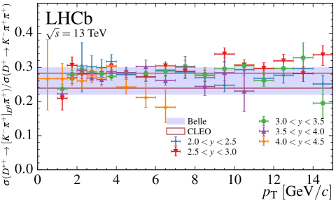
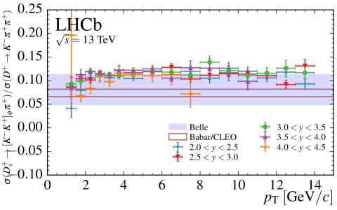
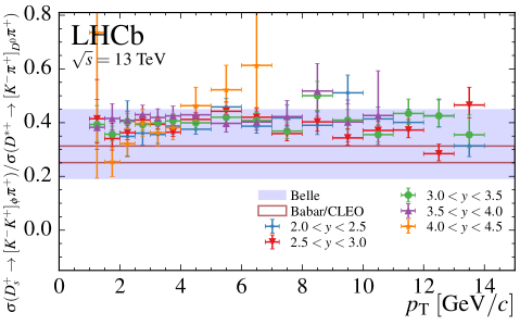
Figure 10: Ratios of cross-section-times-branching-fraction measurements of (top) $D^{*+}$, and (middle) $D_{s}^{+}$ mesons with respect to $D^{+}$ cross-sections, and (bottom) $D_{s}^{+}$ over $D^{*+}$ mesons. The bands indicate the corresponding ratios computed using measurements from $e^{+}e^{-}$ collider experiments [40, 41, 42]. The ratios are given as a function of $p_{\mathrm{T}}$ and different symbols indicate different ranges in $y$. The notation $\sigma(\mbox{$D\to f$})$ is shorthand for $\sigma(D)\times\mathcal{B}(\mbox{$D\to f$})$.

Table 13: The ratios of differential production cross-section-times-branching fraction measurements for prompt $D^{+}$ and $D^{0}$ mesons in bins of $(p_{\mathrm{T}},y)$. The first uncertainty is statistical, and the second is the total systematic. All values are given in percent.    $y$ $p_{\text{T}}$ [MeV/c] $[2,2.5]$ $[2.5,3]$ $[3,3.5]$ $[3.5,4]$ $[4,4.5]$ $[0,1000]$ $132$ ${}^{+}_{-}$ ${}^{5}_{5}$ ${}^{+}_{-}$ ${}^{29}_{23}$ $89$ ${}^{+}_{-}$ ${}^{2}_{2}$ ${}^{+}_{-}$ ${}^{10}_{10}$ $89$ ${}^{+}_{-}$ ${}^{3}_{3}$ ${}^{+}_{-}$ ${}^{10}_{10}$ $82$ ${}^{+}_{-}$ ${}^{5}_{5}$ ${}^{+}_{-}$ ${}^{17}_{16}$ $[1000,1500]$ $99$ ${}^{+}_{-}$ ${}^{4}_{4}$ ${}^{+}_{-}$ ${}^{20}_{19}$ $87.3$ ${}^{+}_{-}$ ${}^{0.9}_{1.0}$ ${}^{+}_{-}$ ${}^{11.8}_{\phantom{0}7.0}$ $95.5$ ${}^{+}_{-}$ ${}^{0.8}_{0.8}$ ${}^{+}_{-}$ ${}^{6.3}_{6.1}$ $91.1$ ${}^{+}_{-}$ ${}^{1.0}_{1.0}$ ${}^{+}_{-}$ ${}^{5.9}_{5.6}$ $95.8$ ${}^{+}_{-}$ ${}^{2.1}_{2.1}$ ${}^{+}_{-}$ ${}^{9.2}_{8.8}$ $[1500,2000]$ $88.3$ ${}^{+}_{-}$ ${}^{1.5}_{1.5}$ ${}^{+}_{-}$ ${}^{9.9}_{9.1}$ $86.1$ ${}^{+}_{-}$ ${}^{0.5}_{0.5}$ ${}^{+}_{-}$ ${}^{8.5}_{6.0}$ $95.1$ ${}^{+}_{-}$ ${}^{0.5}_{0.5}$ ${}^{+}_{-}$ ${}^{4.8}_{5.5}$ $91.3$ ${}^{+}_{-}$ ${}^{0.6}_{0.6}$ ${}^{+}_{-}$ ${}^{4.6}_{4.5}$ $95.2$ ${}^{+}_{-}$ ${}^{1.4}_{1.4}$ ${}^{+}_{-}$ ${}^{6.8}_{6.9}$ $[2000,2500]$ $88.0$ ${}^{+}_{-}$ ${}^{1.0}_{1.0}$ ${}^{+}_{-}$ ${}^{8.8}_{7.0}$ $94.4$ ${}^{+}_{-}$ ${}^{0.5}_{0.5}$ ${}^{+}_{-}$ ${}^{7.4}_{5.7}$ $92.9$ ${}^{+}_{-}$ ${}^{0.4}_{0.4}$ ${}^{+}_{-}$ ${}^{3.7}_{4.6}$ $88.4$ ${}^{+}_{-}$ ${}^{0.5}_{0.5}$ ${}^{+}_{-}$ ${}^{3.7}_{3.9}$ $98.0$ ${}^{+}_{-}$ ${}^{1.2}_{1.2}$ ${}^{+}_{-}$ ${}^{6.0}_{5.1}$ $[2500,3000]$ $88.8$ ${}^{+}_{-}$ ${}^{0.9}_{0.9}$ ${}^{+}_{-}$ ${}^{8.2}_{7.0}$ $96.6$ ${}^{+}_{-}$ ${}^{0.5}_{0.5}$ ${}^{+}_{-}$ ${}^{4.5}_{6.5}$ $94.1$ ${}^{+}_{-}$ ${}^{0.4}_{0.4}$ ${}^{+}_{-}$ ${}^{3.5}_{4.3}$ $96.9$ ${}^{+}_{-}$ ${}^{0.6}_{0.6}$ ${}^{+}_{-}$ ${}^{4.0}_{4.7}$ $96.6$ ${}^{+}_{-}$ ${}^{1.2}_{1.2}$ ${}^{+}_{-}$ ${}^{5.8}_{4.6}$ $[3000,3500]$ $90.9$ ${}^{+}_{-}$ ${}^{0.9}_{0.9}$ ${}^{+}_{-}$ ${}^{8.1}_{7.4}$ $100.5$ ${}^{+}_{-}$ ${}^{0.5}_{0.5}$ ${}^{+}_{-}$ ${}^{4.5}_{6.1}$ $101.6$ ${}^{+}_{-}$ ${}^{0.5}_{0.5}$ ${}^{+}_{-}$ ${}^{3.7}_{4.2}$ $96.3$ ${}^{+}_{-}$ ${}^{0.6}_{0.6}$ ${}^{+}_{-}$ ${}^{4.2}_{4.8}$ $96.1$ ${}^{+}_{-}$ ${}^{1.4}_{1.3}$ ${}^{+}_{-}$ ${}^{6.0}_{5.2}$ $[3500,4000]$ $91.0$ ${}^{+}_{-}$ ${}^{0.9}_{0.9}$ ${}^{+}_{-}$ ${}^{7.2}_{7.5}$ $98.4$ ${}^{+}_{-}$ ${}^{0.5}_{0.5}$ ${}^{+}_{-}$ ${}^{4.6}_{5.3}$ $105.7$ ${}^{+}_{-}$ ${}^{0.6}_{0.6}$ ${}^{+}_{-}$ ${}^{4.2}_{4.1}$ $94.8$ ${}^{+}_{-}$ ${}^{0.7}_{0.7}$ ${}^{+}_{-}$ ${}^{4.3}_{4.0}$ $91.8$ ${}^{+}_{-}$ ${}^{1.5}_{1.5}$ ${}^{+}_{-}$ ${}^{7.2}_{7.2}$ $[4000,5000]$ $103.2$ ${}^{+}_{-}$ ${}^{0.8}_{0.8}$ ${}^{+}_{-}$ ${}^{5.9}_{8.7}$ $103.0$ ${}^{+}_{-}$ ${}^{0.5}_{0.5}$ ${}^{+}_{-}$ ${}^{4.3}_{5.0}$ $100.9$ ${}^{+}_{-}$ ${}^{0.5}_{0.5}$ ${}^{+}_{-}$ ${}^{4.0}_{3.3}$ $98.9$ ${}^{+}_{-}$ ${}^{0.7}_{0.6}$ ${}^{+}_{-}$ ${}^{4.6}_{2.7}$ $125$ ${}^{+}_{-}$ ${}^{2}_{2}$ ${}^{+}_{-}$ ${}^{13}_{14}$ $[5000,6000]$ $100.2$ ${}^{+}_{-}$ ${}^{0.9}_{0.9}$ ${}^{+}_{-}$ ${}^{4.9}_{8.1}$ $108.2$ ${}^{+}_{-}$ ${}^{0.6}_{0.6}$ ${}^{+}_{-}$ ${}^{4.6}_{4.8}$ $105.6$ ${}^{+}_{-}$ ${}^{0.7}_{0.7}$ ${}^{+}_{-}$ ${}^{4.7}_{3.3}$ $106.6$ ${}^{+}_{-}$ ${}^{1.0}_{1.0}$ ${}^{+}_{-}$ ${}^{4.6}_{4.2}$ $149$ ${}^{+}_{-}$ ${}^{6}_{6}$ ${}^{+}_{-}$ ${}^{26}_{27}$ $[6000,7000]$ $106.0$ ${}^{+}_{-}$ ${}^{1.1}_{1.1}$ ${}^{+}_{-}$ ${}^{5.5}_{7.6}$ $101.1$ ${}^{+}_{-}$ ${}^{0.8}_{0.8}$ ${}^{+}_{-}$ ${}^{4.5}_{4.3}$ $103.0$ ${}^{+}_{-}$ ${}^{0.9}_{0.9}$ ${}^{+}_{-}$ ${}^{5.1}_{3.3}$ $112.8$ ${}^{+}_{-}$ ${}^{1.6}_{1.5}$ ${}^{+}_{-}$ ${}^{7.7}_{8.3}$ $210$ ${}^{+}_{-}$ ${}^{40}_{30}$ ${}^{+}_{-}$ ${}^{130}_{\phantom{0}90}$ $[7000,8000]$ $115.5$ ${}^{+}_{-}$ ${}^{1.6}_{1.5}$ ${}^{+}_{-}$ ${}^{6.9}_{7.8}$ $102.8$ ${}^{+}_{-}$ ${}^{1.0}_{1.0}$ ${}^{+}_{-}$ ${}^{4.7}_{4.7}$ $104.8$ ${}^{+}_{-}$ ${}^{1.2}_{1.2}$ ${}^{+}_{-}$ ${}^{6.1}_{3.6}$ $122$ ${}^{+}_{-}$ ${}^{3}_{3}$ ${}^{+}_{-}$ ${}^{12}_{14}$ $[8000,9000]$ $119.5$ ${}^{+}_{-}$ ${}^{2.0}_{1.9}$ ${}^{+}_{-}$ ${}^{8.5}_{7.6}$ $108.2$ ${}^{+}_{-}$ ${}^{1.4}_{1.4}$ ${}^{+}_{-}$ ${}^{5.6}_{5.7}$ $113.0$ ${}^{+}_{-}$ ${}^{1.7}_{1.7}$ ${}^{+}_{-}$ ${}^{7.2}_{5.0}$ $114$ ${}^{+}_{-}$ ${}^{5}_{5}$ ${}^{+}_{-}$ ${}^{17}_{17}$ $[9000,10000]$ $87.8$ ${}^{+}_{-}$ ${}^{1.8}_{1.7}$ ${}^{+}_{-}$ ${}^{4.8}_{4.2}$ $91.0$ ${}^{+}_{-}$ ${}^{1.5}_{1.5}$ ${}^{+}_{-}$ ${}^{3.5}_{3.8}$ $102.0$ ${}^{+}_{-}$ ${}^{2.1}_{2.0}$ ${}^{+}_{-}$ ${}^{3.2}_{4.4}$ $143$ ${}^{+}_{-}$ ${}^{12}_{11}$ ${}^{+}_{-}$ ${}^{24}_{28}$ $[10000,11000]$ $108.4$ ${}^{+}_{-}$ ${}^{2.7}_{2.7}$ ${}^{+}_{-}$ ${}^{5.3}_{4.5}$ $104.7$ ${}^{+}_{-}$ ${}^{2.2}_{2.2}$ ${}^{+}_{-}$ ${}^{2.7}_{4.1}$ $113.7$ ${}^{+}_{-}$ ${}^{3.2}_{3.1}$ ${}^{+}_{-}$ ${}^{4.2}_{6.8}$ $146$ ${}^{+}_{-}$ ${}^{32}_{23}$ ${}^{+}_{-}$ ${}^{32}_{32}$ $[11000,12000]$ $114.9$ ${}^{+}_{-}$ ${}^{3.6}_{3.4}$ ${}^{+}_{-}$ ${}^{5.5}_{5.2}$ $101.4$ ${}^{+}_{-}$ ${}^{2.7}_{2.6}$ ${}^{+}_{-}$ ${}^{2.6}_{3.8}$ $119.3$ ${}^{+}_{-}$ ${}^{4.9}_{4.4}$ ${}^{+}_{-}$ ${}^{4.8}_{7.3}$ $[12000,13000]$ $119.2$ ${}^{+}_{-}$ ${}^{4.6}_{4.5}$ ${}^{+}_{-}$ ${}^{7.2}_{6.9}$ $101.0$ ${}^{+}_{-}$ ${}^{3.4}_{3.2}$ ${}^{+}_{-}$ ${}^{2.8}_{4.2}$ $110.4$ ${}^{+}_{-}$ ${}^{6.3}_{6.0}$ ${}^{+}_{-}$ ${}^{6.8}_{6.6}$ $[13000,14000]$ $114.2$ ${}^{+}_{-}$ ${}^{5.3}_{5.0}$ ${}^{+}_{-}$ ${}^{6.6}_{6.5}$ $97.8$ ${}^{+}_{-}$ ${}^{4.0}_{3.9}$ ${}^{+}_{-}$ ${}^{4.2}_{4.0}$ $125$ ${}^{+}_{-}$ ${}^{10}_{\phantom{0}9}$ ${}^{+}_{-}$ ${}^{15}_{16}$ $[14000,15000]$ $118.1$ ${}^{+}_{-}$ ${}^{6.9}_{6.3}$ ${}^{+}_{-}$ ${}^{7.2}_{5.7}$ $100.9$ ${}^{+}_{-}$ ${}^{5.2}_{4.9}$ ${}^{+}_{-}$ ${}^{5.9}_{3.8}$ $142$ ${}^{+}_{-}$ ${}^{20}_{16}$ ${}^{+}_{-}$ ${}^{25}_{18}$

Table 14: The ratios of differential production cross-section-times-branching-fraction measurements for prompt $D_{s}^{+}$ and $D^{0}$ mesons in bins of $(p_{\mathrm{T}},y)$. The first uncertainty is statistical, and the second is the total systematic. All values are given in percent.    $y$ $p_{\text{T}}$ [MeV/c] $[2,2.5]$ $[2.5,3]$ $[3,3.5]$ $[3.5,4]$ $[4,4.5]$ $[1000,1500]$ $4.1$ ${}^{+}_{-}$ ${}^{1.0}_{1.0}$ ${}^{+}_{-}$ ${}^{1.8}_{1.6}$ $7.6$ ${}^{+}_{-}$ ${}^{0.5}_{0.5}$ ${}^{+}_{-}$ ${}^{2.3}_{1.4}$ $8.9$ ${}^{+}_{-}$ ${}^{0.5}_{0.5}$ ${}^{+}_{-}$ ${}^{1.4}_{1.4}$ $7.7$ ${}^{+}_{-}$ ${}^{0.8}_{0.8}$ ${}^{+}_{-}$ ${}^{1.9}_{1.5}$ $19$ ${}^{+}_{-}$ ${}^{6}_{6}$ ${}^{+}_{-}$ ${}^{\phantom{0}5}_{12}$ $[1500,2000]$ $7.0$ ${}^{+}_{-}$ ${}^{0.4}_{0.4}$ ${}^{+}_{-}$ ${}^{1.5}_{1.2}$ $9.0$ ${}^{+}_{-}$ ${}^{0.2}_{0.2}$ ${}^{+}_{-}$ ${}^{1.5}_{1.1}$ $9.43$ ${}^{+}_{-}$ ${}^{0.24}_{0.24}$ ${}^{+}_{-}$ ${}^{0.72}_{0.78}$ $10.3$ ${}^{+}_{-}$ ${}^{0.4}_{0.4}$ ${}^{+}_{-}$ ${}^{1.0}_{1.0}$ $6.5$ ${}^{+}_{-}$ ${}^{0.7}_{0.7}$ ${}^{+}_{-}$ ${}^{1.1}_{1.1}$ $[2000,2500]$ $9.3$ ${}^{+}_{-}$ ${}^{0.3}_{0.3}$ ${}^{+}_{-}$ ${}^{1.6}_{1.2}$ $9.59$ ${}^{+}_{-}$ ${}^{0.17}_{0.17}$ ${}^{+}_{-}$ ${}^{0.99}_{0.65}$ $11.07$ ${}^{+}_{-}$ ${}^{0.19}_{0.19}$ ${}^{+}_{-}$ ${}^{0.66}_{0.70}$ $10.50$ ${}^{+}_{-}$ ${}^{0.25}_{0.25}$ ${}^{+}_{-}$ ${}^{0.71}_{0.74}$ $8.2$ ${}^{+}_{-}$ ${}^{0.5}_{0.5}$ ${}^{+}_{-}$ ${}^{1.1}_{1.0}$ $[2500,3000]$ $9.7$ ${}^{+}_{-}$ ${}^{0.3}_{0.3}$ ${}^{+}_{-}$ ${}^{1.4}_{1.1}$ $11.12$ ${}^{+}_{-}$ ${}^{0.16}_{0.16}$ ${}^{+}_{-}$ ${}^{0.58}_{0.90}$ $10.59$ ${}^{+}_{-}$ ${}^{0.15}_{0.15}$ ${}^{+}_{-}$ ${}^{0.61}_{0.50}$ $11.19$ ${}^{+}_{-}$ ${}^{0.22}_{0.23}$ ${}^{+}_{-}$ ${}^{0.65}_{0.73}$ $10.6$ ${}^{+}_{-}$ ${}^{0.5}_{0.5}$ ${}^{+}_{-}$ ${}^{1.1}_{1.1}$ $[3000,3500]$ $9.7$ ${}^{+}_{-}$ ${}^{0.3}_{0.3}$ ${}^{+}_{-}$ ${}^{1.2}_{1.0}$ $11.13$ ${}^{+}_{-}$ ${}^{0.16}_{0.17}$ ${}^{+}_{-}$ ${}^{0.57}_{0.78}$ $11.36$ ${}^{+}_{-}$ ${}^{0.17}_{0.17}$ ${}^{+}_{-}$ ${}^{0.62}_{0.51}$ $10.66$ ${}^{+}_{-}$ ${}^{0.22}_{0.21}$ ${}^{+}_{-}$ ${}^{0.62}_{0.70}$ $9.40$ ${}^{+}_{-}$ ${}^{0.46}_{0.46}$ ${}^{+}_{-}$ ${}^{0.96}_{0.87}$ $[3500,4000]$ $11.2$ ${}^{+}_{-}$ ${}^{0.3}_{0.3}$ ${}^{+}_{-}$ ${}^{1.2}_{1.0}$ $10.88$ ${}^{+}_{-}$ ${}^{0.17}_{0.17}$ ${}^{+}_{-}$ ${}^{0.55}_{0.72}$ $11.72$ ${}^{+}_{-}$ ${}^{0.19}_{0.19}$ ${}^{+}_{-}$ ${}^{0.60}_{0.54}$ $11.58$ ${}^{+}_{-}$ ${}^{0.25}_{0.25}$ ${}^{+}_{-}$ ${}^{0.73}_{0.71}$ $10.6$ ${}^{+}_{-}$ ${}^{0.6}_{0.6}$ ${}^{+}_{-}$ ${}^{1.3}_{1.1}$ $[4000,5000]$ $10.80$ ${}^{+}_{-}$ ${}^{0.22}_{0.21}$ ${}^{+}_{-}$ ${}^{0.90}_{0.97}$ $12.01$ ${}^{+}_{-}$ ${}^{0.15}_{0.15}$ ${}^{+}_{-}$ ${}^{0.60}_{0.61}$ $11.37$ ${}^{+}_{-}$ ${}^{0.15}_{0.15}$ ${}^{+}_{-}$ ${}^{0.48}_{0.42}$ $12.08$ ${}^{+}_{-}$ ${}^{0.22}_{0.22}$ ${}^{+}_{-}$ ${}^{0.57}_{0.54}$ $14.0$ ${}^{+}_{-}$ ${}^{0.7}_{0.6}$ ${}^{+}_{-}$ ${}^{2.1}_{1.7}$ $[5000,6000]$ $12.5$ ${}^{+}_{-}$ ${}^{0.3}_{0.3}$ ${}^{+}_{-}$ ${}^{0.8}_{1.2}$ $13.02$ ${}^{+}_{-}$ ${}^{0.21}_{0.20}$ ${}^{+}_{-}$ ${}^{0.77}_{0.58}$ $12.53$ ${}^{+}_{-}$ ${}^{0.22}_{0.22}$ ${}^{+}_{-}$ ${}^{0.65}_{0.51}$ $12.79$ ${}^{+}_{-}$ ${}^{0.30}_{0.29}$ ${}^{+}_{-}$ ${}^{0.88}_{0.67}$ $16.5$ ${}^{+}_{-}$ ${}^{1.2}_{1.2}$ ${}^{+}_{-}$ ${}^{2.8}_{2.7}$ $[6000,7000]$ $11.95$ ${}^{+}_{-}$ ${}^{0.33}_{0.33}$ ${}^{+}_{-}$ ${}^{0.81}_{1.00}$ $12.94$ ${}^{+}_{-}$ ${}^{0.27}_{0.26}$ ${}^{+}_{-}$ ${}^{0.77}_{0.62}$ $12.15$ ${}^{+}_{-}$ ${}^{0.28}_{0.27}$ ${}^{+}_{-}$ ${}^{0.73}_{0.59}$ $11.86$ ${}^{+}_{-}$ ${}^{0.40}_{0.39}$ ${}^{+}_{-}$ ${}^{0.96}_{0.66}$ $23$ ${}^{+}_{-}$ ${}^{5}_{4}$ ${}^{+}_{-}$ ${}^{15}_{10}$ $[7000,8000]$ $13.8$ ${}^{+}_{-}$ ${}^{0.5}_{0.5}$ ${}^{+}_{-}$ ${}^{1.2}_{1.1}$ $10.64$ ${}^{+}_{-}$ ${}^{0.29}_{0.29}$ ${}^{+}_{-}$ ${}^{0.58}_{0.68}$ $11.71$ ${}^{+}_{-}$ ${}^{0.35}_{0.34}$ ${}^{+}_{-}$ ${}^{0.94}_{0.62}$ $15.5$ ${}^{+}_{-}$ ${}^{0.8}_{0.8}$ ${}^{+}_{-}$ ${}^{2.2}_{1.8}$ $[8000,9000]$ $12.6$ ${}^{+}_{-}$ ${}^{0.5}_{0.5}$ ${}^{+}_{-}$ ${}^{1.3}_{1.1}$ $12.06$ ${}^{+}_{-}$ ${}^{0.41}_{0.41}$ ${}^{+}_{-}$ ${}^{0.84}_{0.93}$ $15.7$ ${}^{+}_{-}$ ${}^{0.6}_{0.6}$ ${}^{+}_{-}$ ${}^{1.6}_{1.2}$ $14.5$ ${}^{+}_{-}$ ${}^{1.1}_{1.1}$ ${}^{+}_{-}$ ${}^{3.0}_{2.6}$ $[9000,10000]$ $11.11$ ${}^{+}_{-}$ ${}^{0.56}_{0.55}$ ${}^{+}_{-}$ ${}^{0.96}_{0.74}$ $10.60$ ${}^{+}_{-}$ ${}^{0.46}_{0.45}$ ${}^{+}_{-}$ ${}^{0.57}_{0.57}$ $12.35$ ${}^{+}_{-}$ ${}^{0.61}_{0.59}$ ${}^{+}_{-}$ ${}^{0.79}_{0.65}$ $16.3$ ${}^{+}_{-}$ ${}^{2.1}_{1.9}$ ${}^{+}_{-}$ ${}^{3.7}_{3.7}$ $[10000,11000]$ $12.84$ ${}^{+}_{-}$ ${}^{0.80}_{0.78}$ ${}^{+}_{-}$ ${}^{0.82}_{0.23}$ $11.92$ ${}^{+}_{-}$ ${}^{0.63}_{0.63}$ ${}^{+}_{-}$ ${}^{0.24}_{0.36}$ $12.30$ ${}^{+}_{-}$ ${}^{0.82}_{0.82}$ ${}^{+}_{-}$ ${}^{0.77}_{0.14}$ $14.5$ ${}^{+}_{-}$ ${}^{4.1}_{3.2}$ ${}^{+}_{-}$ ${}^{4.8}_{3.9}$ $[11000,12000]$ $12.05$ ${}^{+}_{-}$ ${}^{0.94}_{0.94}$ ${}^{+}_{-}$ ${}^{0.69}_{0.33}$ $11.21$ ${}^{+}_{-}$ ${}^{0.74}_{0.74}$ ${}^{+}_{-}$ ${}^{0.42}_{0.27}$ $13.5$ ${}^{+}_{-}$ ${}^{1.1}_{1.1}$ ${}^{+}_{-}$ ${}^{1.0}_{0.4}$ $[12000,13000]$ $14.0$ ${}^{+}_{-}$ ${}^{1.2}_{1.2}$ ${}^{+}_{-}$ ${}^{0.9}_{0.6}$ $9.17$ ${}^{+}_{-}$ ${}^{0.81}_{0.80}$ ${}^{+}_{-}$ ${}^{0.43}_{0.25}$ $14.0$ ${}^{+}_{-}$ ${}^{1.5}_{1.4}$ ${}^{+}_{-}$ ${}^{1.0}_{1.0}$ $[13000,14000]$ $10.6$ ${}^{+}_{-}$ ${}^{1.3}_{1.2}$ ${}^{+}_{-}$ ${}^{0.6}_{0.5}$ $12.8$ ${}^{+}_{-}$ ${}^{1.2}_{1.1}$ ${}^{+}_{-}$ ${}^{0.8}_{0.3}$ $14.1$ ${}^{+}_{-}$ ${}^{2.2}_{2.0}$ ${}^{+}_{-}$ ${}^{1.9}_{0.2}$ $[14000,15000]$

Table 15: The ratios of differential production cross-section-times-branching-fraction measurements for prompt $D^{*+}$ and $D^{0}$ mesons in bins of $(p_{\mathrm{T}},y)$. The first uncertainty is statistical, and the second is the total systematic. All values are given in percent.    $y$ $p_{\text{T}}$ [MeV/c] $[2,2.5]$ $[2.5,3]$ $[3,3.5]$ $[3.5,4]$ $[4,4.5]$ $[0,1000]$ $21.9$ ${}^{+}_{-}$ ${}^{3.0}_{3.0}$ ${}^{+}_{-}$ ${}^{6.7}_{6.3}$ $[1000,1500]$ $18.3$ ${}^{+}_{-}$ ${}^{0.8}_{0.8}$ ${}^{+}_{-}$ ${}^{2.0}_{2.0}$ $22.6$ ${}^{+}_{-}$ ${}^{0.3}_{0.3}$ ${}^{+}_{-}$ ${}^{1.3}_{1.6}$ $20.3$ ${}^{+}_{-}$ ${}^{0.3}_{0.3}$ ${}^{+}_{-}$ ${}^{1.4}_{1.5}$ $25.5$ ${}^{+}_{-}$ ${}^{0.8}_{0.8}$ ${}^{+}_{-}$ ${}^{3.7}_{3.1}$ $[1500,2000]$ $26.3$ ${}^{+}_{-}$ ${}^{0.5}_{0.4}$ ${}^{+}_{-}$ ${}^{1.8}_{1.6}$ $26.4$ ${}^{+}_{-}$ ${}^{0.2}_{0.2}$ ${}^{+}_{-}$ ${}^{1.3}_{1.9}$ $24.7$ ${}^{+}_{-}$ ${}^{0.3}_{0.3}$ ${}^{+}_{-}$ ${}^{1.5}_{1.9}$ $25.5$ ${}^{+}_{-}$ ${}^{0.6}_{0.6}$ ${}^{+}_{-}$ ${}^{2.5}_{2.0}$ $[2000,2500]$ $26.8$ ${}^{+}_{-}$ ${}^{2.4}_{2.4}$ ${}^{+}_{-}$ ${}^{5.7}_{6.0}$ $26.5$ ${}^{+}_{-}$ ${}^{0.3}_{0.3}$ ${}^{+}_{-}$ ${}^{1.9}_{1.1}$ $27.4$ ${}^{+}_{-}$ ${}^{0.2}_{0.2}$ ${}^{+}_{-}$ ${}^{1.3}_{1.8}$ $25.7$ ${}^{+}_{-}$ ${}^{0.2}_{0.2}$ ${}^{+}_{-}$ ${}^{1.6}_{1.6}$ $25.5$ ${}^{+}_{-}$ ${}^{0.5}_{0.5}$ ${}^{+}_{-}$ ${}^{2.6}_{2.1}$ $[2500,3000]$ $26.8$ ${}^{+}_{-}$ ${}^{0.9}_{0.9}$ ${}^{+}_{-}$ ${}^{2.9}_{3.1}$ $27.1$ ${}^{+}_{-}$ ${}^{0.3}_{0.3}$ ${}^{+}_{-}$ ${}^{1.2}_{1.7}$ $27.0$ ${}^{+}_{-}$ ${}^{0.2}_{0.2}$ ${}^{+}_{-}$ ${}^{1.6}_{1.5}$ $26.0$ ${}^{+}_{-}$ ${}^{0.2}_{0.3}$ ${}^{+}_{-}$ ${}^{1.7}_{1.7}$ $26.6$ ${}^{+}_{-}$ ${}^{0.6}_{0.6}$ ${}^{+}_{-}$ ${}^{1.8}_{2.0}$ $[3000,3500]$ $27.2$ ${}^{+}_{-}$ ${}^{0.7}_{0.7}$ ${}^{+}_{-}$ ${}^{2.2}_{2.5}$ $28.3$ ${}^{+}_{-}$ ${}^{0.2}_{0.2}$ ${}^{+}_{-}$ ${}^{1.2}_{1.9}$ $28.6$ ${}^{+}_{-}$ ${}^{0.2}_{0.2}$ ${}^{+}_{-}$ ${}^{1.7}_{1.4}$ $25.5$ ${}^{+}_{-}$ ${}^{0.3}_{0.3}$ ${}^{+}_{-}$ ${}^{1.8}_{1.8}$ $25.9$ ${}^{+}_{-}$ ${}^{0.6}_{0.6}$ ${}^{+}_{-}$ ${}^{2.7}_{2.2}$ $[3500,4000]$ $28.9$ ${}^{+}_{-}$ ${}^{0.6}_{0.6}$ ${}^{+}_{-}$ ${}^{2.1}_{2.5}$ $29.8$ ${}^{+}_{-}$ ${}^{0.3}_{0.3}$ ${}^{+}_{-}$ ${}^{1.4}_{2.1}$ $28.9$ ${}^{+}_{-}$ ${}^{0.2}_{0.2}$ ${}^{+}_{-}$ ${}^{1.8}_{1.4}$ $27.2$ ${}^{+}_{-}$ ${}^{0.3}_{0.3}$ ${}^{+}_{-}$ ${}^{1.9}_{1.7}$ $27.9$ ${}^{+}_{-}$ ${}^{0.8}_{0.8}$ ${}^{+}_{-}$ ${}^{2.7}_{2.7}$ $[4000,5000]$ $28.8$ ${}^{+}_{-}$ ${}^{0.4}_{0.4}$ ${}^{+}_{-}$ ${}^{1.4}_{2.3}$ $29.2$ ${}^{+}_{-}$ ${}^{0.2}_{0.2}$ ${}^{+}_{-}$ ${}^{1.3}_{2.0}$ $28.5$ ${}^{+}_{-}$ ${}^{0.2}_{0.2}$ ${}^{+}_{-}$ ${}^{1.6}_{1.4}$ $28.2$ ${}^{+}_{-}$ ${}^{0.3}_{0.3}$ ${}^{+}_{-}$ ${}^{2.0}_{1.5}$ $30.3$ ${}^{+}_{-}$ ${}^{0.9}_{0.9}$ ${}^{+}_{-}$ ${}^{2.3}_{2.2}$ $[5000,6000]$ $27.3$ ${}^{+}_{-}$ ${}^{0.4}_{0.4}$ ${}^{+}_{-}$ ${}^{1.3}_{2.3}$ $29.4$ ${}^{+}_{-}$ ${}^{0.2}_{0.2}$ ${}^{+}_{-}$ ${}^{1.4}_{2.0}$ $29.9$ ${}^{+}_{-}$ ${}^{0.3}_{0.3}$ ${}^{+}_{-}$ ${}^{1.7}_{1.3}$ $32.2$ ${}^{+}_{-}$ ${}^{0.4}_{0.5}$ ${}^{+}_{-}$ ${}^{2.3}_{1.6}$ $31.5$ ${}^{+}_{-}$ ${}^{2.1}_{2.0}$ ${}^{+}_{-}$ ${}^{4.1}_{3.7}$ $[6000,7000]$ $30.9$ ${}^{+}_{-}$ ${}^{0.5}_{0.5}$ ${}^{+}_{-}$ ${}^{1.8}_{2.6}$ $30.8$ ${}^{+}_{-}$ ${}^{0.3}_{0.3}$ ${}^{+}_{-}$ ${}^{1.6}_{2.1}$ $29.8$ ${}^{+}_{-}$ ${}^{0.4}_{0.4}$ ${}^{+}_{-}$ ${}^{1.7}_{1.5}$ $29.5$ ${}^{+}_{-}$ ${}^{0.6}_{0.6}$ ${}^{+}_{-}$ ${}^{2.2}_{2.2}$ $38$ ${}^{+}_{-}$ ${}^{10}_{\phantom{0}8}$ ${}^{+}_{-}$ ${}^{24}_{17}$ $[7000,8000]$ $33.1$ ${}^{+}_{-}$ ${}^{0.7}_{0.7}$ ${}^{+}_{-}$ ${}^{2.0}_{2.9}$ $29.6$ ${}^{+}_{-}$ ${}^{0.4}_{0.4}$ ${}^{+}_{-}$ ${}^{1.7}_{2.3}$ $31.7$ ${}^{+}_{-}$ ${}^{0.5}_{0.5}$ ${}^{+}_{-}$ ${}^{2.2}_{1.6}$ $36.8$ ${}^{+}_{-}$ ${}^{1.3}_{1.2}$ ${}^{+}_{-}$ ${}^{4.4}_{4.3}$ $[8000,9000]$ $32.2$ ${}^{+}_{-}$ ${}^{0.8}_{0.8}$ ${}^{+}_{-}$ ${}^{2.2}_{2.9}$ $29.9$ ${}^{+}_{-}$ ${}^{0.5}_{0.5}$ ${}^{+}_{-}$ ${}^{1.9}_{2.3}$ $31.4$ ${}^{+}_{-}$ ${}^{0.7}_{0.7}$ ${}^{+}_{-}$ ${}^{2.8}_{1.7}$ $28.0$ ${}^{+}_{-}$ ${}^{1.8}_{1.7}$ ${}^{+}_{-}$ ${}^{4.1}_{3.4}$ $[9000,10000]$ $21.8$ ${}^{+}_{-}$ ${}^{0.7}_{0.7}$ ${}^{+}_{-}$ ${}^{1.2}_{1.7}$ $30.9$ ${}^{+}_{-}$ ${}^{0.7}_{0.7}$ ${}^{+}_{-}$ ${}^{1.6}_{2.1}$ $30.2$ ${}^{+}_{-}$ ${}^{0.8}_{0.8}$ ${}^{+}_{-}$ ${}^{1.6}_{1.5}$ $40.6$ ${}^{+}_{-}$ ${}^{4.8}_{4.3}$ ${}^{+}_{-}$ ${}^{6.1}_{7.0}$ $[10000,11000]$ $31.8$ ${}^{+}_{-}$ ${}^{1.2}_{1.1}$ ${}^{+}_{-}$ ${}^{1.6}_{2.2}$ $32.1$ ${}^{+}_{-}$ ${}^{0.9}_{0.9}$ ${}^{+}_{-}$ ${}^{1.6}_{2.1}$ $34.6$ ${}^{+}_{-}$ ${}^{1.4}_{1.3}$ ${}^{+}_{-}$ ${}^{1.8}_{1.8}$ $34$ ${}^{+}_{-}$ ${}^{10}_{\phantom{0}8}$ ${}^{+}_{-}$ ${}^{13}_{11}$ $[11000,12000]$ $30.8$ ${}^{+}_{-}$ ${}^{1.3}_{1.4}$ ${}^{+}_{-}$ ${}^{1.6}_{2.5}$ $30.1$ ${}^{+}_{-}$ ${}^{1.1}_{1.1}$ ${}^{+}_{-}$ ${}^{1.4}_{2.0}$ $31.2$ ${}^{+}_{-}$ ${}^{1.8}_{1.7}$ ${}^{+}_{-}$ ${}^{1.6}_{1.7}$ $[12000,13000]$ $33.0$ ${}^{+}_{-}$ ${}^{1.8}_{1.8}$ ${}^{+}_{-}$ ${}^{2.1}_{3.1}$ $32.2$ ${}^{+}_{-}$ ${}^{1.4}_{1.4}$ ${}^{+}_{-}$ ${}^{1.6}_{2.2}$ $32.8$ ${}^{+}_{-}$ ${}^{2.5}_{2.4}$ ${}^{+}_{-}$ ${}^{2.2}_{1.8}$ $[13000,14000]$ $34.0$ ${}^{+}_{-}$ ${}^{2.1}_{2.1}$ ${}^{+}_{-}$ ${}^{1.8}_{3.0}$ $27.6$ ${}^{+}_{-}$ ${}^{1.6}_{1.6}$ ${}^{+}_{-}$ ${}^{1.5}_{2.0}$ $41.2$ ${}^{+}_{-}$ ${}^{4.7}_{4.3}$ ${}^{+}_{-}$ ${}^{3.1}_{3.4}$ $[14000,15000]$ $29.7$ ${}^{+}_{-}$ ${}^{2.5}_{2.4}$ ${}^{+}_{-}$ ${}^{1.9}_{2.4}$ $34.0$ ${}^{+}_{-}$ ${}^{2.5}_{2.3}$ ${}^{+}_{-}$ ${}^{2.3}_{2.5}$ $27.8$ ${}^{+}_{-}$ ${}^{5.6}_{4.8}$ ${}^{+}_{-}$ ${}^{6.7}_{5.7}$

Table 16: The ratios of differential production cross-section-times-branching-fraction measurements for prompt $D_{s}^{+}$ and $D^{+}$ mesons in bins of $(p_{\mathrm{T}},y)$. The first uncertainty is statistical, and the second is the total systematic. All values are given in percent.    $y$ $p_{\text{T}}$ [MeV/c] $[2,2.5]$ $[2.5,3]$ $[3,3.5]$ $[3.5,4]$ $[4,4.5]$ $[1000,1500]$ $4.1$ ${}^{+}_{-}$ ${}^{1.0}_{1.0}$ ${}^{+}_{-}$ ${}^{2.0}_{1.7}$ $8.7$ ${}^{+}_{-}$ ${}^{0.6}_{0.6}$ ${}^{+}_{-}$ ${}^{1.9}_{1.5}$ $9.3$ ${}^{+}_{-}$ ${}^{0.6}_{0.6}$ ${}^{+}_{-}$ ${}^{1.4}_{1.4}$ $8.5$ ${}^{+}_{-}$ ${}^{0.8}_{0.8}$ ${}^{+}_{-}$ ${}^{2.0}_{1.6}$ $20$ ${}^{+}_{-}$ ${}^{6}_{6}$ ${}^{+}_{-}$ ${}^{\phantom{0}5}_{13}$ $[1500,2000]$ $8.0$ ${}^{+}_{-}$ ${}^{0.5}_{0.5}$ ${}^{+}_{-}$ ${}^{1.5}_{1.2}$ $10.42$ ${}^{+}_{-}$ ${}^{0.28}_{0.28}$ ${}^{+}_{-}$ ${}^{0.98}_{0.86}$ $9.92$ ${}^{+}_{-}$ ${}^{0.25}_{0.25}$ ${}^{+}_{-}$ ${}^{0.68}_{0.67}$ $11.2$ ${}^{+}_{-}$ ${}^{0.4}_{0.4}$ ${}^{+}_{-}$ ${}^{1.1}_{1.0}$ $6.8$ ${}^{+}_{-}$ ${}^{0.7}_{0.7}$ ${}^{+}_{-}$ ${}^{1.2}_{1.2}$ $[2000,2500]$ $10.6$ ${}^{+}_{-}$ ${}^{0.4}_{0.4}$ ${}^{+}_{-}$ ${}^{1.4}_{1.1}$ $10.15$ ${}^{+}_{-}$ ${}^{0.18}_{0.18}$ ${}^{+}_{-}$ ${}^{0.58}_{0.42}$ $11.93$ ${}^{+}_{-}$ ${}^{0.20}_{0.21}$ ${}^{+}_{-}$ ${}^{0.64}_{0.56}$ $11.88$ ${}^{+}_{-}$ ${}^{0.28}_{0.28}$ ${}^{+}_{-}$ ${}^{0.76}_{0.76}$ $8.4$ ${}^{+}_{-}$ ${}^{0.5}_{0.6}$ ${}^{+}_{-}$ ${}^{1.1}_{1.0}$ $[2500,3000]$ $10.9$ ${}^{+}_{-}$ ${}^{0.3}_{0.3}$ ${}^{+}_{-}$ ${}^{1.2}_{0.9}$ $11.51$ ${}^{+}_{-}$ ${}^{0.17}_{0.17}$ ${}^{+}_{-}$ ${}^{0.44}_{0.52}$ $11.25$ ${}^{+}_{-}$ ${}^{0.17}_{0.16}$ ${}^{+}_{-}$ ${}^{0.60}_{0.36}$ $11.55$ ${}^{+}_{-}$ ${}^{0.23}_{0.23}$ ${}^{+}_{-}$ ${}^{0.65}_{0.64}$ $10.9$ ${}^{+}_{-}$ ${}^{0.5}_{0.5}$ ${}^{+}_{-}$ ${}^{1.1}_{1.2}$ $[3000,3500]$ $10.66$ ${}^{+}_{-}$ ${}^{0.30}_{0.29}$ ${}^{+}_{-}$ ${}^{0.93}_{0.70}$ $11.07$ ${}^{+}_{-}$ ${}^{0.16}_{0.17}$ ${}^{+}_{-}$ ${}^{0.42}_{0.45}$ $11.18$ ${}^{+}_{-}$ ${}^{0.17}_{0.17}$ ${}^{+}_{-}$ ${}^{0.56}_{0.39}$ $11.07$ ${}^{+}_{-}$ ${}^{0.22}_{0.22}$ ${}^{+}_{-}$ ${}^{0.59}_{0.58}$ $9.77$ ${}^{+}_{-}$ ${}^{0.48}_{0.48}$ ${}^{+}_{-}$ ${}^{0.93}_{0.88}$ $[3500,4000]$ $12.27$ ${}^{+}_{-}$ ${}^{0.33}_{0.33}$ ${}^{+}_{-}$ ${}^{0.95}_{0.67}$ $11.05$ ${}^{+}_{-}$ ${}^{0.17}_{0.17}$ ${}^{+}_{-}$ ${}^{0.43}_{0.49}$ $11.09$ ${}^{+}_{-}$ ${}^{0.18}_{0.18}$ ${}^{+}_{-}$ ${}^{0.54}_{0.46}$ $12.21$ ${}^{+}_{-}$ ${}^{0.27}_{0.26}$ ${}^{+}_{-}$ ${}^{0.69}_{0.69}$ $11.6$ ${}^{+}_{-}$ ${}^{0.6}_{0.6}$ ${}^{+}_{-}$ ${}^{1.3}_{1.0}$ $[4000,5000]$ $10.47$ ${}^{+}_{-}$ ${}^{0.21}_{0.21}$ ${}^{+}_{-}$ ${}^{0.66}_{0.41}$ $11.66$ ${}^{+}_{-}$ ${}^{0.15}_{0.15}$ ${}^{+}_{-}$ ${}^{0.46}_{0.36}$ $11.27$ ${}^{+}_{-}$ ${}^{0.15}_{0.15}$ ${}^{+}_{-}$ ${}^{0.42}_{0.42}$ $12.21$ ${}^{+}_{-}$ ${}^{0.22}_{0.22}$ ${}^{+}_{-}$ ${}^{0.45}_{0.63}$ $11.2$ ${}^{+}_{-}$ ${}^{0.5}_{0.5}$ ${}^{+}_{-}$ ${}^{1.1}_{0.7}$ $[5000,6000]$ $12.49$ ${}^{+}_{-}$ ${}^{0.29}_{0.29}$ ${}^{+}_{-}$ ${}^{0.70}_{0.65}$ $12.03$ ${}^{+}_{-}$ ${}^{0.19}_{0.19}$ ${}^{+}_{-}$ ${}^{0.62}_{0.41}$ $11.87$ ${}^{+}_{-}$ ${}^{0.20}_{0.20}$ ${}^{+}_{-}$ ${}^{0.51}_{0.54}$ $12.00$ ${}^{+}_{-}$ ${}^{0.28}_{0.27}$ ${}^{+}_{-}$ ${}^{0.81}_{0.63}$ $11.1$ ${}^{+}_{-}$ ${}^{0.7}_{0.7}$ ${}^{+}_{-}$ ${}^{1.4}_{1.2}$ $[6000,7000]$ $11.28$ ${}^{+}_{-}$ ${}^{0.31}_{0.31}$ ${}^{+}_{-}$ ${}^{0.71}_{0.65}$ $12.80$ ${}^{+}_{-}$ ${}^{0.26}_{0.26}$ ${}^{+}_{-}$ ${}^{0.70}_{0.57}$ $11.80$ ${}^{+}_{-}$ ${}^{0.27}_{0.27}$ ${}^{+}_{-}$ ${}^{0.62}_{0.66}$ $10.51$ ${}^{+}_{-}$ ${}^{0.34}_{0.33}$ ${}^{+}_{-}$ ${}^{0.99}_{0.62}$ $11.2$ ${}^{+}_{-}$ ${}^{1.3}_{1.3}$ ${}^{+}_{-}$ ${}^{2.0}_{1.7}$ $[7000,8000]$ $12.0$ ${}^{+}_{-}$ ${}^{0.4}_{0.4}$ ${}^{+}_{-}$ ${}^{1.0}_{0.8}$ $10.35$ ${}^{+}_{-}$ ${}^{0.28}_{0.27}$ ${}^{+}_{-}$ ${}^{0.58}_{0.65}$ $11.17$ ${}^{+}_{-}$ ${}^{0.33}_{0.33}$ ${}^{+}_{-}$ ${}^{0.74}_{0.69}$ $12.7$ ${}^{+}_{-}$ ${}^{0.6}_{0.6}$ ${}^{+}_{-}$ ${}^{1.4}_{0.9}$ $7.2$ ${}^{+}_{-}$ ${}^{2.0}_{1.9}$ ${}^{+}_{-}$ ${}^{2.7}_{2.2}$ $[8000,9000]$ $10.53$ ${}^{+}_{-}$ ${}^{0.43}_{0.44}$ ${}^{+}_{-}$ ${}^{0.98}_{0.91}$ $11.15$ ${}^{+}_{-}$ ${}^{0.38}_{0.38}$ ${}^{+}_{-}$ ${}^{0.81}_{0.83}$ $13.9$ ${}^{+}_{-}$ ${}^{0.5}_{0.5}$ ${}^{+}_{-}$ ${}^{1.2}_{1.2}$ $12.7$ ${}^{+}_{-}$ ${}^{0.9}_{0.8}$ ${}^{+}_{-}$ ${}^{1.8}_{1.3}$ $[9000,10000]$ $12.6$ ${}^{+}_{-}$ ${}^{0.6}_{0.6}$ ${}^{+}_{-}$ ${}^{1.1}_{0.8}$ $11.65$ ${}^{+}_{-}$ ${}^{0.49}_{0.50}$ ${}^{+}_{-}$ ${}^{0.76}_{0.66}$ $12.11$ ${}^{+}_{-}$ ${}^{0.58}_{0.58}$ ${}^{+}_{-}$ ${}^{0.92}_{0.62}$ $11.4$ ${}^{+}_{-}$ ${}^{1.1}_{1.1}$ ${}^{+}_{-}$ ${}^{1.2}_{1.0}$ $[10000,11000]$ $11.98$ ${}^{+}_{-}$ ${}^{0.72}_{0.72}$ ${}^{+}_{-}$ ${}^{0.37}_{0.36}$ $11.38$ ${}^{+}_{-}$ ${}^{0.59}_{0.61}$ ${}^{+}_{-}$ ${}^{0.43}_{0.17}$ $11.07$ ${}^{+}_{-}$ ${}^{0.70}_{0.71}$ ${}^{+}_{-}$ ${}^{0.60}_{0.59}$ $9.9$ ${}^{+}_{-}$ ${}^{1.8}_{1.7}$ ${}^{+}_{-}$ ${}^{1.1}_{0.7}$ $[11000,12000]$ $10.58$ ${}^{+}_{-}$ ${}^{0.80}_{0.81}$ ${}^{+}_{-}$ ${}^{0.36}_{0.35}$ $11.05$ ${}^{+}_{-}$ ${}^{0.73}_{0.71}$ ${}^{+}_{-}$ ${}^{0.52}_{0.14}$ $11.57$ ${}^{+}_{-}$ ${}^{0.89}_{0.89}$ ${}^{+}_{-}$ ${}^{0.45}_{0.44}$ $[12000,13000]$ $11.8$ ${}^{+}_{-}$ ${}^{1.0}_{1.0}$ ${}^{+}_{-}$ ${}^{0.6}_{0.2}$ $9.17$ ${}^{+}_{-}$ ${}^{0.79}_{0.78}$ ${}^{+}_{-}$ ${}^{0.38}_{0.38}$ $12.6$ ${}^{+}_{-}$ ${}^{1.2}_{1.2}$ ${}^{+}_{-}$ ${}^{0.6}_{0.6}$ $[13000,14000]$ $9.3$ ${}^{+}_{-}$ ${}^{1.1}_{1.1}$ ${}^{+}_{-}$ ${}^{0.4}_{0.4}$ $13.1$ ${}^{+}_{-}$ ${}^{1.2}_{1.2}$ ${}^{+}_{-}$ ${}^{0.8}_{0.2}$ $11.7$ ${}^{+}_{-}$ ${}^{1.6}_{1.6}$ ${}^{+}_{-}$ ${}^{1.1}_{1.0}$ $[14000,15000]$

Table 17: The ratios of differential production cross-section-times-branching-fraction for prompt $D^{*+}$ and $D^{+}$ mesons in bins of $(p_{\mathrm{T}},y)$. The first uncertainty is statistical, and the second is the total systematic. All values are given in percent.    $y$ $p_{\text{T}}$ [MeV/c] $[2,2.5]$ $[2.5,3]$ $[3,3.5]$ $[3.5,4]$ $[4,4.5]$ $[0,1000]$ $27$ ${}^{+}_{-}$ ${}^{4}_{4}$ ${}^{+}_{-}$ ${}^{11}_{\phantom{0}8}$ $[1000,1500]$ $20.9$ ${}^{+}_{-}$ ${}^{0.9}_{0.9}$ ${}^{+}_{-}$ ${}^{2.5}_{3.3}$ $23.7$ ${}^{+}_{-}$ ${}^{0.3}_{0.4}$ ${}^{+}_{-}$ ${}^{1.4}_{1.6}$ $22.3$ ${}^{+}_{-}$ ${}^{0.4}_{0.4}$ ${}^{+}_{-}$ ${}^{1.5}_{1.6}$ $26.7$ ${}^{+}_{-}$ ${}^{1.0}_{1.0}$ ${}^{+}_{-}$ ${}^{4.4}_{3.4}$ $[1500,2000]$ $30.6$ ${}^{+}_{-}$ ${}^{0.5}_{0.5}$ ${}^{+}_{-}$ ${}^{2.4}_{2.8}$ $27.8$ ${}^{+}_{-}$ ${}^{0.2}_{0.2}$ ${}^{+}_{-}$ ${}^{1.3}_{1.6}$ $27.0$ ${}^{+}_{-}$ ${}^{0.3}_{0.3}$ ${}^{+}_{-}$ ${}^{1.5}_{1.8}$ $26.8$ ${}^{+}_{-}$ ${}^{0.7}_{0.6}$ ${}^{+}_{-}$ ${}^{2.7}_{2.0}$ $[2000,2500]$ $30.4$ ${}^{+}_{-}$ ${}^{2.8}_{2.7}$ ${}^{+}_{-}$ ${}^{6.3}_{7.1}$ $28.0$ ${}^{+}_{-}$ ${}^{0.3}_{0.3}$ ${}^{+}_{-}$ ${}^{1.7}_{1.2}$ $29.5$ ${}^{+}_{-}$ ${}^{0.2}_{0.2}$ ${}^{+}_{-}$ ${}^{1.2}_{1.4}$ $29.1$ ${}^{+}_{-}$ ${}^{0.3}_{0.3}$ ${}^{+}_{-}$ ${}^{1.6}_{1.4}$ $26.0$ ${}^{+}_{-}$ ${}^{0.5}_{0.5}$ ${}^{+}_{-}$ ${}^{2.4}_{2.1}$ $[2500,3000]$ $30.2$ ${}^{+}_{-}$ ${}^{1.1}_{1.1}$ ${}^{+}_{-}$ ${}^{3.0}_{3.5}$ $28.1$ ${}^{+}_{-}$ ${}^{0.3}_{0.3}$ ${}^{+}_{-}$ ${}^{1.0}_{1.0}$ $28.7$ ${}^{+}_{-}$ ${}^{0.2}_{0.2}$ ${}^{+}_{-}$ ${}^{1.5}_{1.1}$ $26.9$ ${}^{+}_{-}$ ${}^{0.3}_{0.3}$ ${}^{+}_{-}$ ${}^{1.6}_{1.4}$ $27.5$ ${}^{+}_{-}$ ${}^{0.6}_{0.6}$ ${}^{+}_{-}$ ${}^{1.6}_{1.9}$ $[3000,3500]$ $29.9$ ${}^{+}_{-}$ ${}^{0.8}_{0.8}$ ${}^{+}_{-}$ ${}^{2.2}_{2.6}$ $28.1$ ${}^{+}_{-}$ ${}^{0.2}_{0.3}$ ${}^{+}_{-}$ ${}^{0.8}_{1.0}$ $28.1$ ${}^{+}_{-}$ ${}^{0.2}_{0.2}$ ${}^{+}_{-}$ ${}^{1.5}_{1.0}$ $26.4$ ${}^{+}_{-}$ ${}^{0.3}_{0.3}$ ${}^{+}_{-}$ ${}^{1.6}_{1.4}$ $27.0$ ${}^{+}_{-}$ ${}^{0.6}_{0.6}$ ${}^{+}_{-}$ ${}^{2.8}_{2.4}$ $[3500,4000]$ $31.7$ ${}^{+}_{-}$ ${}^{0.7}_{0.7}$ ${}^{+}_{-}$ ${}^{2.0}_{2.2}$ $30.3$ ${}^{+}_{-}$ ${}^{0.3}_{0.3}$ ${}^{+}_{-}$ ${}^{0.8}_{1.2}$ $27.3$ ${}^{+}_{-}$ ${}^{0.2}_{0.2}$ ${}^{+}_{-}$ ${}^{1.4}_{1.0}$ $28.7$ ${}^{+}_{-}$ ${}^{0.3}_{0.3}$ ${}^{+}_{-}$ ${}^{1.7}_{1.6}$ $30.4$ ${}^{+}_{-}$ ${}^{0.8}_{0.8}$ ${}^{+}_{-}$ ${}^{2.1}_{2.0}$ $[4000,5000]$ $27.9$ ${}^{+}_{-}$ ${}^{0.4}_{0.4}$ ${}^{+}_{-}$ ${}^{1.3}_{1.3}$ $28.3$ ${}^{+}_{-}$ ${}^{0.2}_{0.2}$ ${}^{+}_{-}$ ${}^{0.7}_{1.2}$ $28.2$ ${}^{+}_{-}$ ${}^{0.2}_{0.2}$ ${}^{+}_{-}$ ${}^{1.2}_{1.1}$ $28.5$ ${}^{+}_{-}$ ${}^{0.3}_{0.3}$ ${}^{+}_{-}$ ${}^{1.6}_{1.6}$ $24.3$ ${}^{+}_{-}$ ${}^{0.7}_{0.7}$ ${}^{+}_{-}$ ${}^{2.7}_{1.9}$ $[5000,6000]$ $27.2$ ${}^{+}_{-}$ ${}^{0.4}_{0.4}$ ${}^{+}_{-}$ ${}^{1.2}_{1.2}$ $27.2$ ${}^{+}_{-}$ ${}^{0.2}_{0.2}$ ${}^{+}_{-}$ ${}^{0.8}_{1.3}$ $28.3$ ${}^{+}_{-}$ ${}^{0.2}_{0.2}$ ${}^{+}_{-}$ ${}^{1.3}_{1.3}$ $30.2$ ${}^{+}_{-}$ ${}^{0.4}_{0.4}$ ${}^{+}_{-}$ ${}^{1.9}_{1.3}$ $21.2$ ${}^{+}_{-}$ ${}^{1.2}_{1.2}$ ${}^{+}_{-}$ ${}^{4.0}_{2.7}$ $[6000,7000]$ $29.2$ ${}^{+}_{-}$ ${}^{0.5}_{0.5}$ ${}^{+}_{-}$ ${}^{1.4}_{1.5}$ $30.5$ ${}^{+}_{-}$ ${}^{0.3}_{0.3}$ ${}^{+}_{-}$ ${}^{1.1}_{1.6}$ $28.9$ ${}^{+}_{-}$ ${}^{0.3}_{0.3}$ ${}^{+}_{-}$ ${}^{1.2}_{1.5}$ $26.1$ ${}^{+}_{-}$ ${}^{0.5}_{0.5}$ ${}^{+}_{-}$ ${}^{1.6}_{1.3}$ $18.3$ ${}^{+}_{-}$ ${}^{3.0}_{3.0}$ ${}^{+}_{-}$ ${}^{4.0}_{3.4}$ $[7000,8000]$ $28.7$ ${}^{+}_{-}$ ${}^{0.6}_{0.6}$ ${}^{+}_{-}$ ${}^{1.4}_{1.9}$ $28.8$ ${}^{+}_{-}$ ${}^{0.4}_{0.4}$ ${}^{+}_{-}$ ${}^{1.4}_{1.8}$ $30.3$ ${}^{+}_{-}$ ${}^{0.5}_{0.5}$ ${}^{+}_{-}$ ${}^{1.6}_{1.6}$ $30.1$ ${}^{+}_{-}$ ${}^{0.9}_{0.9}$ ${}^{+}_{-}$ ${}^{3.0}_{2.3}$ $[8000,9000]$ $27.0$ ${}^{+}_{-}$ ${}^{0.7}_{0.7}$ ${}^{+}_{-}$ ${}^{1.4}_{2.2}$ $27.7$ ${}^{+}_{-}$ ${}^{0.5}_{0.5}$ ${}^{+}_{-}$ ${}^{1.4}_{1.8}$ $27.8$ ${}^{+}_{-}$ ${}^{0.6}_{0.5}$ ${}^{+}_{-}$ ${}^{2.1}_{1.6}$ $24.4$ ${}^{+}_{-}$ ${}^{1.2}_{1.2}$ ${}^{+}_{-}$ ${}^{3.8}_{2.4}$ $[9000,10000]$ $24.7$ ${}^{+}_{-}$ ${}^{0.8}_{0.8}$ ${}^{+}_{-}$ ${}^{1.1}_{1.7}$ $33.9$ ${}^{+}_{-}$ ${}^{0.7}_{0.7}$ ${}^{+}_{-}$ ${}^{1.7}_{2.0}$ $29.6$ ${}^{+}_{-}$ ${}^{0.8}_{0.8}$ ${}^{+}_{-}$ ${}^{1.7}_{1.3}$ $28.4$ ${}^{+}_{-}$ ${}^{2.6}_{2.5}$ ${}^{+}_{-}$ ${}^{3.6}_{2.8}$ $[10000,11000]$ $29.3$ ${}^{+}_{-}$ ${}^{1.0}_{1.0}$ ${}^{+}_{-}$ ${}^{0.6}_{1.5}$ $30.7$ ${}^{+}_{-}$ ${}^{0.8}_{0.8}$ ${}^{+}_{-}$ ${}^{1.3}_{1.5}$ $30.5$ ${}^{+}_{-}$ ${}^{1.1}_{1.0}$ ${}^{+}_{-}$ ${}^{1.4}_{0.3}$ $23.1$ ${}^{+}_{-}$ ${}^{4.2}_{4.1}$ ${}^{+}_{-}$ ${}^{4.8}_{4.3}$ $[11000,12000]$ $26.8$ ${}^{+}_{-}$ ${}^{1.2}_{1.1}$ ${}^{+}_{-}$ ${}^{0.8}_{1.6}$ $29.7$ ${}^{+}_{-}$ ${}^{1.0}_{1.0}$ ${}^{+}_{-}$ ${}^{1.3}_{1.6}$ $26.1$ ${}^{+}_{-}$ ${}^{1.3}_{1.3}$ ${}^{+}_{-}$ ${}^{1.9}_{1.2}$ $[12000,13000]$ $27.7$ ${}^{+}_{-}$ ${}^{1.4}_{1.4}$ ${}^{+}_{-}$ ${}^{1.0}_{1.9}$ $31.9$ ${}^{+}_{-}$ ${}^{1.3}_{1.3}$ ${}^{+}_{-}$ ${}^{1.5}_{1.7}$ $29.7$ ${}^{+}_{-}$ ${}^{2.0}_{2.0}$ ${}^{+}_{-}$ ${}^{1.7}_{1.1}$ $[13000,14000]$ $29.7$ ${}^{+}_{-}$ ${}^{1.8}_{1.7}$ ${}^{+}_{-}$ ${}^{1.2}_{2.3}$ $28.2$ ${}^{+}_{-}$ ${}^{1.6}_{1.5}$ ${}^{+}_{-}$ ${}^{1.3}_{1.8}$ $32.8$ ${}^{+}_{-}$ ${}^{3.0}_{2.8}$ ${}^{+}_{-}$ ${}^{3.2}_{2.0}$ $[14000,15000]$ $25.1$ ${}^{+}_{-}$ ${}^{2.0}_{1.9}$ ${}^{+}_{-}$ ${}^{1.7}_{2.2}$ $33.7$ ${}^{+}_{-}$ ${}^{2.2}_{2.1}$ ${}^{+}_{-}$ ${}^{1.6}_{2.4}$ $19.5$ ${}^{+}_{-}$ ${}^{3.0}_{2.9}$ ${}^{+}_{-}$ ${}^{3.2}_{3.3}$

Table 18: The ratios of differential production cross-section-times-branching-fraction for prompt $D_{s}^{+}$ and $D^{*+}$ mesons in bins of $(p_{\mathrm{T}},y)$. The first uncertainty is statistical, and the second is the total systematic. All values are given in percent.    $y$ $p_{\text{T}}$ [MeV/c] $[2,2.5]$ $[2.5,3]$ $[3,3.5]$ $[3.5,4]$ $[4,4.5]$ $[1000,1500]$ $41$ ${}^{+}_{-}$ ${}^{3}_{3}$ ${}^{+}_{-}$ ${}^{14}_{\phantom{0}8}$ $39.3$ ${}^{+}_{-}$ ${}^{2.4}_{2.4}$ ${}^{+}_{-}$ ${}^{6.6}_{5.8}$ $38.3$ ${}^{+}_{-}$ ${}^{3.9}_{3.8}$ ${}^{+}_{-}$ ${}^{9.6}_{7.2}$ $74$ ${}^{+}_{-}$ ${}^{24}_{24}$ ${}^{+}_{-}$ ${}^{22}_{49}$ $[1500,2000]$ $34.1$ ${}^{+}_{-}$ ${}^{1.1}_{1.0}$ ${}^{+}_{-}$ ${}^{5.6}_{4.1}$ $35.7$ ${}^{+}_{-}$ ${}^{0.9}_{0.9}$ ${}^{+}_{-}$ ${}^{2.9}_{2.4}$ $41.6$ ${}^{+}_{-}$ ${}^{1.5}_{1.5}$ ${}^{+}_{-}$ ${}^{5.2}_{4.1}$ $25.4$ ${}^{+}_{-}$ ${}^{2.7}_{2.6}$ ${}^{+}_{-}$ ${}^{4.6}_{4.8}$ $[2000,2500]$ $35$ ${}^{+}_{-}$ ${}^{4}_{3}$ ${}^{+}_{-}$ ${}^{13}_{\phantom{0}7}$ $36.2$ ${}^{+}_{-}$ ${}^{0.7}_{0.7}$ ${}^{+}_{-}$ ${}^{2.7}_{2.5}$ $40.5$ ${}^{+}_{-}$ ${}^{0.7}_{0.7}$ ${}^{+}_{-}$ ${}^{2.9}_{2.1}$ $40.8$ ${}^{+}_{-}$ ${}^{1.0}_{1.0}$ ${}^{+}_{-}$ ${}^{3.3}_{3.3}$ $32.2$ ${}^{+}_{-}$ ${}^{2.2}_{2.2}$ ${}^{+}_{-}$ ${}^{5.0}_{4.5}$ $[2500,3000]$ $36.1$ ${}^{+}_{-}$ ${}^{1.7}_{1.6}$ ${}^{+}_{-}$ ${}^{6.7}_{4.1}$ $41.0$ ${}^{+}_{-}$ ${}^{0.7}_{0.7}$ ${}^{+}_{-}$ ${}^{1.8}_{2.1}$ $39.3$ ${}^{+}_{-}$ ${}^{0.6}_{0.6}$ ${}^{+}_{-}$ ${}^{2.6}_{2.0}$ $43.0$ ${}^{+}_{-}$ ${}^{0.9}_{0.9}$ ${}^{+}_{-}$ ${}^{3.4}_{3.4}$ $39.7$ ${}^{+}_{-}$ ${}^{2.1}_{2.1}$ ${}^{+}_{-}$ ${}^{4.8}_{4.2}$ $[3000,3500]$ $35.6$ ${}^{+}_{-}$ ${}^{1.3}_{1.3}$ ${}^{+}_{-}$ ${}^{4.9}_{3.1}$ $39.4$ ${}^{+}_{-}$ ${}^{0.7}_{0.6}$ ${}^{+}_{-}$ ${}^{1.8}_{1.6}$ $39.8$ ${}^{+}_{-}$ ${}^{0.6}_{0.6}$ ${}^{+}_{-}$ ${}^{2.3}_{2.3}$ $41.9$ ${}^{+}_{-}$ ${}^{0.9}_{0.9}$ ${}^{+}_{-}$ ${}^{3.1}_{3.2}$ $36.2$ ${}^{+}_{-}$ ${}^{1.9}_{1.9}$ ${}^{+}_{-}$ ${}^{4.7}_{4.5}$ $[3500,4000]$ $38.7$ ${}^{+}_{-}$ ${}^{1.3}_{1.3}$ ${}^{+}_{-}$ ${}^{4.1}_{2.6}$ $36.4$ ${}^{+}_{-}$ ${}^{0.6}_{0.6}$ ${}^{+}_{-}$ ${}^{1.9}_{1.5}$ $40.6$ ${}^{+}_{-}$ ${}^{0.7}_{0.7}$ ${}^{+}_{-}$ ${}^{2.4}_{2.5}$ $42.5$ ${}^{+}_{-}$ ${}^{1.0}_{1.0}$ ${}^{+}_{-}$ ${}^{3.5}_{3.3}$ $38.1$ ${}^{+}_{-}$ ${}^{2.3}_{2.3}$ ${}^{+}_{-}$ ${}^{4.8}_{3.8}$ $[4000,5000]$ $37.6$ ${}^{+}_{-}$ ${}^{0.9}_{0.9}$ ${}^{+}_{-}$ ${}^{2.8}_{1.8}$ $41.2$ ${}^{+}_{-}$ ${}^{0.6}_{0.6}$ ${}^{+}_{-}$ ${}^{2.4}_{1.2}$ $39.9$ ${}^{+}_{-}$ ${}^{0.6}_{0.6}$ ${}^{+}_{-}$ ${}^{2.1}_{2.2}$ $42.9$ ${}^{+}_{-}$ ${}^{0.8}_{0.8}$ ${}^{+}_{-}$ ${}^{2.7}_{3.0}$ $46.3$ ${}^{+}_{-}$ ${}^{2.4}_{2.3}$ ${}^{+}_{-}$ ${}^{6.4}_{5.2}$ $[5000,6000]$ $45.8$ ${}^{+}_{-}$ ${}^{1.2}_{1.2}$ ${}^{+}_{-}$ ${}^{2.9}_{2.7}$ $44.2$ ${}^{+}_{-}$ ${}^{0.8}_{0.8}$ ${}^{+}_{-}$ ${}^{3.4}_{1.5}$ $42.0$ ${}^{+}_{-}$ ${}^{0.8}_{0.8}$ ${}^{+}_{-}$ ${}^{2.5}_{2.4}$ $39.7$ ${}^{+}_{-}$ ${}^{1.0}_{1.0}$ ${}^{+}_{-}$ ${}^{3.1}_{3.1}$ $52.2$ ${}^{+}_{-}$ ${}^{4.6}_{4.2}$ ${}^{+}_{-}$ ${}^{7.9}_{7.8}$ $[6000,7000]$ $38.7$ ${}^{+}_{-}$ ${}^{1.2}_{1.2}$ ${}^{+}_{-}$ ${}^{2.9}_{2.3}$ $42.0$ ${}^{+}_{-}$ ${}^{0.9}_{0.9}$ ${}^{+}_{-}$ ${}^{3.4}_{2.0}$ $40.8$ ${}^{+}_{-}$ ${}^{1.0}_{1.0}$ ${}^{+}_{-}$ ${}^{2.9}_{2.5}$ $40.2$ ${}^{+}_{-}$ ${}^{1.5}_{1.4}$ ${}^{+}_{-}$ ${}^{3.8}_{2.6}$ $61$ ${}^{+}_{-}$ ${}^{14}_{11}$ ${}^{+}_{-}$ ${}^{19}_{12}$ $[7000,8000]$ $41.7$ ${}^{+}_{-}$ ${}^{1.6}_{1.6}$ ${}^{+}_{-}$ ${}^{4.5}_{2.6}$ $35.9$ ${}^{+}_{-}$ ${}^{1.0}_{1.0}$ ${}^{+}_{-}$ ${}^{3.1}_{2.5}$ $36.9$ ${}^{+}_{-}$ ${}^{1.2}_{1.1}$ ${}^{+}_{-}$ ${}^{3.0}_{2.5}$ $42.3$ ${}^{+}_{-}$ ${}^{2.3}_{2.2}$ ${}^{+}_{-}$ ${}^{5.5}_{4.2}$ $[8000,9000]$ $39.0$ ${}^{+}_{-}$ ${}^{1.8}_{1.7}$ ${}^{+}_{-}$ ${}^{4.6}_{3.1}$ $40.3$ ${}^{+}_{-}$ ${}^{1.5}_{1.4}$ ${}^{+}_{-}$ ${}^{3.9}_{3.2}$ $50.0$ ${}^{+}_{-}$ ${}^{2.0}_{2.0}$ ${}^{+}_{-}$ ${}^{4.9}_{5.1}$ $51.8$ ${}^{+}_{-}$ ${}^{4.2}_{4.0}$ ${}^{+}_{-}$ ${}^{9.3}_{8.5}$ $[9000,10000]$ $51.1$ ${}^{+}_{-}$ ${}^{2.8}_{2.8}$ ${}^{+}_{-}$ ${}^{6.0}_{3.1}$ $34.3$ ${}^{+}_{-}$ ${}^{1.5}_{1.5}$ ${}^{+}_{-}$ ${}^{3.1}_{2.2}$ $40.9$ ${}^{+}_{-}$ ${}^{2.1}_{2.1}$ ${}^{+}_{-}$ ${}^{3.4}_{2.8}$ $40.2$ ${}^{+}_{-}$ ${}^{5.5}_{4.8}$ ${}^{+}_{-}$ ${}^{6.1}_{5.5}$ $[10000,11000]$ $41.4$ ${}^{+}_{-}$ ${}^{2.7}_{2.7}$ ${}^{+}_{-}$ ${}^{2.1}_{2.1}$ $37.1$ ${}^{+}_{-}$ ${}^{2.1}_{2.1}$ ${}^{+}_{-}$ ${}^{2.6}_{1.6}$ $35.5$ ${}^{+}_{-}$ ${}^{2.5}_{2.5}$ ${}^{+}_{-}$ ${}^{2.8}_{1.2}$ $43$ ${}^{+}_{-}$ ${}^{12}_{\phantom{0}9}$ ${}^{+}_{-}$ ${}^{11}_{\phantom{0}5}$ $[11000,12000]$ $40.1$ ${}^{+}_{-}$ ${}^{3.3}_{3.2}$ ${}^{+}_{-}$ ${}^{2.4}_{2.4}$ $37.3$ ${}^{+}_{-}$ ${}^{2.6}_{2.6}$ ${}^{+}_{-}$ ${}^{3.0}_{1.3}$ $43.4$ ${}^{+}_{-}$ ${}^{3.9}_{3.7}$ ${}^{+}_{-}$ ${}^{3.7}_{1.7}$ $[12000,13000]$ $42.5$ ${}^{+}_{-}$ ${}^{4.1}_{3.8}$ ${}^{+}_{-}$ ${}^{4.3}_{1.2}$ $28.4$ ${}^{+}_{-}$ ${}^{2.6}_{2.5}$ ${}^{+}_{-}$ ${}^{2.5}_{0.9}$ $42.6$ ${}^{+}_{-}$ ${}^{4.7}_{4.6}$ ${}^{+}_{-}$ ${}^{2.5}_{2.5}$ $[13000,14000]$ $31.4$ ${}^{+}_{-}$ ${}^{4.0}_{3.9}$ ${}^{+}_{-}$ ${}^{3.3}_{1.0}$ $46.5$ ${}^{+}_{-}$ ${}^{4.7}_{4.5}$ ${}^{+}_{-}$ ${}^{4.7}_{1.5}$ $35.5$ ${}^{+}_{-}$ ${}^{5.5}_{5.4}$ ${}^{+}_{-}$ ${}^{2.8}_{2.7}$ $[14000,15000]$

LHCb collaboration

R. Aaij³⁸, C. Abellán Beteta⁴⁰, B. Adeva³⁷, M. Adinolfi⁴⁶, A. Affolder⁵², Z. Ajaltouni⁵, S. Akar⁶, J. Albrecht⁹, F. Alessio³⁸, M. Alexander⁵¹, S. Ali⁴¹, G. Alkhazov³⁰, P. Alvarez Cartelle⁵³, A.A. Alves Jr⁵⁷, S. Amato², S. Amerio²², Y. Amhis⁷, L. An³, L. Anderlini¹⁷, J. Anderson⁴⁰, G. Andreassi³⁹, M. Andreotti^16,f, J.E. Andrews⁵⁸, R.B. Appleby⁵⁴, O. Aquines Gutierrez¹⁰, F. Archilli³⁸, P. d’Argent¹¹, A. Artamonov³⁵, M. Artuso⁵⁹, E. Aslanides⁶, G. Auriemma^25,m, M. Baalouch⁵, S. Bachmann¹¹, J.J. Back⁴⁸, A. Badalov³⁶, C. Baesso⁶⁰, W. Baldini^16,38, R.J. Barlow⁵⁴, C. Barschel³⁸, S. Barsuk⁷, W. Barter³⁸, V. Batozskaya²⁸, V. Battista³⁹, A. Bay³⁹, L. Beaucourt⁴, J. Beddow⁵¹, F. Bedeschi²³, I. Bediaga¹, L.J. Bel⁴¹, V. Bellee³⁹, N. Belloli^20,j, I. Belyaev³¹, E. Ben-Haim⁸, G. Bencivenni¹⁸, S. Benson³⁸, J. Benton⁴⁶, A. Berezhnoy³², R. Bernet⁴⁰, A. Bertolin²², M.-O. Bettler³⁸, M. van Beuzekom⁴¹, A. Bien¹¹, S. Bifani⁴⁵, P. Billoir⁸, T. Bird⁵⁴, A. Birnkraut⁹, A. Bizzeti^17,h, T. Blake⁴⁸, F. Blanc³⁹, J. Blouw¹⁰, S. Blusk⁵⁹, V. Bocci²⁵, A. Bondar³⁴, N. Bondar^30,38, W. Bonivento¹⁵, S. Borghi⁵⁴, M. Borsato⁷, T.J.V. Bowcock⁵², E. Bowen⁴⁰, C. Bozzi¹⁶, S. Braun¹¹, M. Britsch¹⁰, T. Britton⁵⁹, J. Brodzicka⁵⁴, N.H. Brook⁴⁶, E. Buchanan⁴⁶, C. Burr^49,54, A. Bursche⁴⁰, J. Buytaert³⁸, S. Cadeddu¹⁵, R. Calabrese^16,f, M. Calvi^20,j, M. Calvo Gomez^36,o, P. Campana¹⁸, D. Campora Perez³⁸, L. Capriotti⁵⁴, A. Carbone^14,d, G. Carboni^24,k, R. Cardinale^19,i, A. Cardini¹⁵, P. Carniti^20,j, L. Carson⁵⁰, K. Carvalho Akiba^2,38, G. Casse⁵², L. Cassina^20,j, L. Castillo Garcia³⁸, M. Cattaneo³⁸, Ch. Cauet⁹, G. Cavallero¹⁹, R. Cenci^23,s, M. Charles⁸, Ph. Charpentier³⁸, M. Chefdeville⁴, S. Chen⁵⁴, S.-F. Cheung⁵⁵, N. Chiapolini⁴⁰, M. Chrzaszcz⁴⁰, X. Cid Vidal³⁸, G. Ciezarek⁴¹, P.E.L. Clarke⁵⁰, M. Clemencic³⁸, H.V. Cliff⁴⁷, J. Closier³⁸, V. Coco³⁸, J. Cogan⁶, E. Cogneras⁵, V. Cogoni^15,e, L. Cojocariu²⁹, G. Collazuol²², P. Collins³⁸, A. Comerma-Montells¹¹, A. Contu¹⁵, A. Cook⁴⁶, M. Coombes⁴⁶, S. Coquereau⁸, G. Corti³⁸, M. Corvo^16,f, B. Couturier³⁸, G.A. Cowan⁵⁰, D.C. Craik⁴⁸, A. Crocombe⁴⁸, M. Cruz Torres⁶⁰, S. Cunliffe⁵³, R. Currie⁵³, C. D’Ambrosio³⁸, E. Dall’Occo⁴¹, J. Dalseno⁴⁶, P.N.Y. David⁴¹, A. Davis⁵⁷, O. De Aguiar Francisco², K. De Bruyn⁶, S. De Capua⁵⁴, M. De Cian¹¹, J.M. De Miranda¹, L. De Paula², P. De Simone¹⁸, C.-T. Dean⁵¹, D. Decamp⁴, M. Deckenhoff⁹, L. Del Buono⁸, N. Déléage⁴, M. Demmer⁹, D. Derkach⁶⁵, O. Deschamps⁵, F. Dettori³⁸, B. Dey²¹, A. Di Canto³⁸, F. Di Ruscio²⁴, H. Dijkstra³⁸, S. Donleavy⁵², F. Dordei¹¹, M. Dorigo³⁹, A. Dosil Suárez³⁷, D. Dossett⁴⁸, A. Dovbnya⁴³, K. Dreimanis⁵², L. Dufour⁴¹, G. Dujany⁵⁴, F. Dupertuis³⁹, P. Durante³⁸, R. Dzhelyadin³⁵, A. Dziurda²⁶, A. Dzyuba³⁰, S. Easo^49,38, U. Egede⁵³, V. Egorychev³¹, S. Eidelman³⁴, S. Eisenhardt⁵⁰, U. Eitschberger⁹, R. Ekelhof⁹, L. Eklund⁵¹, I. El Rifai⁵, Ch. Elsasser⁴⁰, S. Ely⁵⁹, S. Esen¹¹, H.M. Evans⁴⁷, T. Evans⁵⁵, A. Falabella¹⁴, C. Färber³⁸, N. Farley⁴⁵, S. Farry⁵², R. Fay⁵², D. Ferguson⁵⁰, V. Fernandez Albor³⁷, F. Ferrari¹⁴, F. Ferreira Rodrigues¹, M. Ferro-Luzzi³⁸, S. Filippov³³, M. Fiore^16,38,f, M. Fiorini^16,f, M. Firlej²⁷, C. Fitzpatrick³⁹, T. Fiutowski²⁷, K. Fohl³⁸, P. Fol⁵³, M. Fontana¹⁵, F. Fontanelli^19,i, D. C. Forshaw⁵⁹, R. Forty³⁸, M. Frank³⁸, C. Frei³⁸, M. Frosini¹⁷, J. Fu²¹, E. Furfaro^24,k, A. Gallas Torreira³⁷, D. Galli^14,d, S. Gallorini²², S. Gambetta⁵⁰, M. Gandelman², P. Gandini⁵⁵, Y. Gao³, J. García Pardiñas³⁷, J. Garra Tico⁴⁷, L. Garrido³⁶, D. Gascon³⁶, C. Gaspar³⁸, R. Gauld⁵⁵, L. Gavardi⁹, G. Gazzoni⁵, D. Gerick¹¹, E. Gersabeck¹¹, M. Gersabeck⁵⁴, T. Gershon⁴⁸, Ph. Ghez⁴, S. Gianì³⁹, V. Gibson⁴⁷, O.G. Girard³⁹, L. Giubega²⁹, V.V. Gligorov³⁸, C. Göbel⁶⁰, D. Golubkov³¹, A. Golutvin^53,38, A. Gomes^1,a, C. Gotti^20,j, M. Grabalosa Gándara⁵, R. Graciani Diaz³⁶, L.A. Granado Cardoso³⁸, E. Graugés³⁶, E. Graverini⁴⁰, G. Graziani¹⁷, A. Grecu²⁹, E. Greening⁵⁵, S. Gregson⁴⁷, P. Griffith⁴⁵, L. Grillo¹¹, O. Grünberg⁶³, B. Gui⁵⁹, E. Gushchin³³, Yu. Guz^35,38, T. Gys³⁸, T. Hadavizadeh⁵⁵, C. Hadjivasiliou⁵⁹, G. Haefeli³⁹, C. Haen³⁸, S.C. Haines⁴⁷, S. Hall⁵³, B. Hamilton⁵⁸, X. Han¹¹, S. Hansmann-Menzemer¹¹, N. Harnew⁵⁵, S.T. Harnew⁴⁶, J. Harrison⁵⁴, J. He³⁸, T. Head³⁹, V. Heijne⁴¹, K. Hennessy⁵², P. Henrard⁵, L. Henry⁸, E. van Herwijnen³⁸, M. Heß⁶³, A. Hicheur², D. Hill⁵⁵, M. Hoballah⁵, C. Hombach⁵⁴, W. Hulsbergen⁴¹, T. Humair⁵³, N. Hussain⁵⁵, D. Hutchcroft⁵², D. Hynds⁵¹, M. Idzik²⁷, P. Ilten⁵⁶, R. Jacobsson³⁸, A. Jaeger¹¹, J. Jalocha⁵⁵, E. Jans⁴¹, A. Jawahery⁵⁸, F. Jing³, M. John⁵⁵, D. Johnson³⁸, C.R. Jones⁴⁷, C. Joram³⁸, B. Jost³⁸, N. Jurik⁵⁹, S. Kandybei⁴³, W. Kanso⁶, M. Karacson³⁸, T.M. Karbach^38,†, S. Karodia⁵¹, M. Kecke¹¹, M. Kelsey⁵⁹, I.R. Kenyon⁴⁵, M. Kenzie³⁸, T. Ketel⁴², E. Khairullin⁶⁵, B. Khanji^20,38,j, C. Khurewathanakul³⁹, S. Klaver⁵⁴, K. Klimaszewski²⁸, O. Kochebina⁷, M. Kolpin¹¹, I. Komarov³⁹, R.F. Koopman⁴², P. Koppenburg^41,38, M. Kozeiha⁵, L. Kravchuk³³, K. Kreplin¹¹, M. Kreps⁴⁸, G. Krocker¹¹, P. Krokovny³⁴, F. Kruse⁹, W. Krzemien²⁸, W. Kucewicz^26,n, M. Kucharczyk²⁶, V. Kudryavtsev³⁴, A. K. Kuonen³⁹, K. Kurek²⁸, T. Kvaratskheliya³¹, D. Lacarrere³⁸, G. Lafferty^54,38, A. Lai¹⁵, D. Lambert⁵⁰, G. Lanfranchi¹⁸, C. Langenbruch⁴⁸, B. Langhans³⁸, T. Latham⁴⁸, C. Lazzeroni⁴⁵, R. Le Gac⁶, J. van Leerdam⁴¹, J.-P. Lees⁴, R. Lefèvre⁵, A. Leflat^32,38, J. Lefrançois⁷, E. Lemos Cid³⁷, O. Leroy⁶, T. Lesiak²⁶, B. Leverington¹¹, Y. Li⁷, T. Likhomanenko^65,64, M. Liles⁵², R. Lindner³⁸, C. Linn³⁸, F. Lionetto⁴⁰, B. Liu¹⁵, X. Liu³, D. Loh⁴⁸, I. Longstaff⁵¹, J.H. Lopes², D. Lucchesi^22,q, M. Lucio Martinez³⁷, H. Luo⁵⁰, A. Lupato²², E. Luppi^16,f, O. Lupton⁵⁵, A. Lusiani²³, F. Machefert⁷, F. Maciuc²⁹, O. Maev³⁰, K. Maguire⁵⁴, S. Malde⁵⁵, A. Malinin⁶⁴, G. Manca⁷, G. Mancinelli⁶, P. Manning⁵⁹, A. Mapelli³⁸, J. Maratas⁵, J.F. Marchand⁴, U. Marconi¹⁴, C. Marin Benito³⁶, P. Marino^23,38,s, J. Marks¹¹, G. Martellotti²⁵, M. Martin⁶, M. Martinelli³⁹, D. Martinez Santos³⁷, F. Martinez Vidal⁶⁶, D. Martins Tostes², A. Massafferri¹, R. Matev³⁸, A. Mathad⁴⁸, Z. Mathe³⁸, C. Matteuzzi²⁰, A. Mauri⁴⁰, B. Maurin³⁹, A. Mazurov⁴⁵, M. McCann⁵³, J. McCarthy⁴⁵, A. McNab⁵⁴, R. McNulty¹², B. Meadows⁵⁷, F. Meier⁹, M. Meissner¹¹, D. Melnychuk²⁸, M. Merk⁴¹, E Michielin²², D.A. Milanes⁶², M.-N. Minard⁴, D.S. Mitzel¹¹, J. Molina Rodriguez⁶⁰, I.A. Monroy⁶², S. Monteil⁵, M. Morandin²², P. Morawski²⁷, A. Mordà⁶, M.J. Morello^23,s, J. Moron²⁷, A.B. Morris⁵⁰, R. Mountain⁵⁹, F. Muheim⁵⁰, D. Müller⁵⁴, J. Müller⁹, K. Müller⁴⁰, V. Müller⁹, M. Mussini¹⁴, B. Muster³⁹, P. Naik⁴⁶, T. Nakada³⁹, R. Nandakumar⁴⁹, A. Nandi⁵⁵, I. Nasteva², M. Needham⁵⁰, N. Neri²¹, S. Neubert¹¹, N. Neufeld³⁸, M. Neuner¹¹, A.D. Nguyen³⁹, T.D. Nguyen³⁹, C. Nguyen-Mau^39,p, V. Niess⁵, R. Niet⁹, N. Nikitin³², T. Nikodem¹¹, A. Novoselov³⁵, D.P. O’Hanlon⁴⁸, A. Oblakowska-Mucha²⁷, V. Obraztsov³⁵, S. Ogilvy⁵¹, O. Okhrimenko⁴⁴, R. Oldeman^15,e, C.J.G. Onderwater⁶⁷, B. Osorio Rodrigues¹, J.M. Otalora Goicochea², A. Otto³⁸, P. Owen⁵³, A. Oyanguren⁶⁶, A. Palano^13,c, F. Palombo^21,t, M. Palutan¹⁸, J. Panman³⁸, A. Papanestis⁴⁹, M. Pappagallo⁵¹, L.L. Pappalardo^16,f, C. Pappenheimer⁵⁷, W. Parker⁵⁸, C. Parkes⁵⁴, G. Passaleva¹⁷, G.D. Patel⁵², M. Patel⁵³, C. Patrignani^19,i, A. Pearce^54,49, A. Pellegrino⁴¹, G. Penso^25,l, M. Pepe Altarelli³⁸, S. Perazzini^14,d, P. Perret⁵, L. Pescatore⁴⁵, K. Petridis⁴⁶, A. Petrolini^19,i, M. Petruzzo²¹, E. Picatoste Olloqui³⁶, B. Pietrzyk⁴, T. Pilař⁴⁸, D. Pinci²⁵, A. Pistone¹⁹, A. Piucci¹¹, S. Playfer⁵⁰, M. Plo Casasus³⁷, T. Poikela³⁸, F. Polci⁸, A. Poluektov^48,34, I. Polyakov³¹, E. Polycarpo², A. Popov³⁵, D. Popov^10,38, B. Popovici²⁹, C. Potterat², E. Price⁴⁶, J.D. Price⁵², J. Prisciandaro³⁷, A. Pritchard⁵², C. Prouve⁴⁶, V. Pugatch⁴⁴, A. Puig Navarro³⁹, G. Punzi^23,r, W. Qian⁴, R. Quagliani^7,46, B. Rachwal²⁶, J.H. Rademacker⁴⁶, M. Rama²³, M.S. Rangel², I. Raniuk⁴³, N. Rauschmayr³⁸, G. Raven⁴², F. Redi⁵³, S. Reichert⁵⁴, M.M. Reid⁴⁸, A.C. dos Reis¹, S. Ricciardi⁴⁹, S. Richards⁴⁶, M. Rihl³⁸, K. Rinnert^52,38, V. Rives Molina³⁶, P. Robbe^7,38, A.B. Rodrigues¹, E. Rodrigues⁵⁴, J.A. Rodriguez Lopez⁶², P. Rodriguez Perez⁵⁴, S. Roiser³⁸, V. Romanovsky³⁵, A. Romero Vidal³⁷, J. W. Ronayne¹², M. Rotondo²², J. Rouvinet³⁹, T. Ruf³⁸, P. Ruiz Valls⁶⁶, J.J. Saborido Silva³⁷, N. Sagidova³⁰, P. Sail⁵¹, B. Saitta^15,e, V. Salustino Guimaraes², C. Sanchez Mayordomo⁶⁶, B. Sanmartin Sedes³⁷, R. Santacesaria²⁵, C. Santamarina Rios³⁷, M. Santimaria¹⁸, E. Santovetti^24,k, A. Sarti^18,l, C. Satriano^25,m, A. Satta²⁴, D.M. Saunders⁴⁶, D. Savrina^31,32, M. Schiller³⁸, H. Schindler³⁸, M. Schlupp⁹, M. Schmelling¹⁰, T. Schmelzer⁹, B. Schmidt³⁸, O. Schneider³⁹, A. Schopper³⁸, M. Schubiger³⁹, M.-H. Schune⁷, R. Schwemmer³⁸, B. Sciascia¹⁸, A. Sciubba^25,l, A. Semennikov³¹, N. Serra⁴⁰, J. Serrano⁶, L. Sestini²², P. Seyfert²⁰, M. Shapkin³⁵, I. Shapoval^16,43,f, Y. Shcheglov³⁰, T. Shears⁵², L. Shekhtman³⁴, V. Shevchenko⁶⁴, A. Shires⁹, B.G. Siddi¹⁶, R. Silva Coutinho⁴⁰, L. Silva de Oliveira², G. Simi²², M. Sirendi⁴⁷, N. Skidmore⁴⁶, T. Skwarnicki⁵⁹, E. Smith^55,49, E. Smith⁵³, I.T. Smith⁵⁰, J. Smith⁴⁷, M. Smith⁵⁴, H. Snoek⁴¹, M.D. Sokoloff^57,38, F.J.P. Soler⁵¹, F. Soomro³⁹, D. Souza⁴⁶, B. Souza De Paula², B. Spaan⁹, P. Spradlin⁵¹, S. Sridharan³⁸, F. Stagni³⁸, M. Stahl¹¹, S. Stahl³⁸, S. Stefkova⁵³, O. Steinkamp⁴⁰, O. Stenyakin³⁵, S. Stevenson⁵⁵, S. Stoica²⁹, S. Stone⁵⁹, B. Storaci⁴⁰, S. Stracka^23,s, M. Straticiuc²⁹, U. Straumann⁴⁰, L. Sun⁵⁷, W. Sutcliffe⁵³, K. Swientek²⁷, S. Swientek⁹, V. Syropoulos⁴², M. Szczekowski²⁸, T. Szumlak²⁷, S. T’Jampens⁴, A. Tayduganov⁶, T. Tekampe⁹, M. Teklishyn⁷, G. Tellarini^16,f, F. Teubert³⁸, C. Thomas⁵⁵, E. Thomas³⁸, J. van Tilburg⁴¹, V. Tisserand⁴, M. Tobin³⁹, J. Todd⁵⁷, S. Tolk⁴², L. Tomassetti^16,f, D. Tonelli³⁸, S. Topp-Joergensen⁵⁵, N. Torr⁵⁵, E. Tournefier⁴, S. Tourneur³⁹, K. Trabelsi³⁹, M.T. Tran³⁹, M. Tresch⁴⁰, A. Trisovic³⁸, A. Tsaregorodtsev⁶, P. Tsopelas⁴¹, N. Tuning^41,38, A. Ukleja²⁸, A. Ustyuzhanin^65,64, U. Uwer¹¹, C. Vacca^15,38,e, V. Vagnoni¹⁴, G. Valenti¹⁴, A. Vallier⁷, R. Vazquez Gomez¹⁸, P. Vazquez Regueiro³⁷, C. Vázquez Sierra³⁷, S. Vecchi¹⁶, J.J. Velthuis⁴⁶, M. Veltri^17,g, G. Veneziano³⁹, M. Vesterinen¹¹, B. Viaud⁷, D. Vieira², M. Vieites Diaz³⁷, X. Vilasis-Cardona^36,o, V. Volkov³², A. Vollhardt⁴⁰, D. Volyanskyy¹⁰, D. Voong⁴⁶, A. Vorobyev³⁰, V. Vorobyev³⁴, C. Voß⁶³, J.A. de Vries⁴¹, R. Waldi⁶³, C. Wallace⁴⁸, R. Wallace¹², J. Walsh²³, S. Wandernoth¹¹, J. Wang⁵⁹, D.R. Ward⁴⁷, N.K. Watson⁴⁵, D. Websdale⁵³, A. Weiden⁴⁰, M. Whitehead⁴⁸, G. Wilkinson^55,38, M. Wilkinson⁵⁹, M. Williams³⁸, M.P. Williams⁴⁵, M. Williams⁵⁶, T. Williams⁴⁵, F.F. Wilson⁴⁹, J. Wimberley⁵⁸, J. Wishahi⁹, W. Wislicki²⁸, M. Witek²⁶, G. Wormser⁷, S.A. Wotton⁴⁷, K. Wyllie³⁸, Y. Xie⁶¹, Z. Xu³⁹, Z. Yang³, J. Yu⁶¹, X. Yuan³⁴, O. Yushchenko³⁵, M. Zangoli¹⁴, M. Zavertyaev^10,b, L. Zhang³, Y. Zhang³, A. Zhelezov¹¹, A. Zhokhov³¹, L. Zhong³, S. Zucchelli¹⁴.

¹Centro Brasileiro de Pesquisas Físicas (CBPF), Rio de Janeiro, Brazil
²Universidade Federal do Rio de Janeiro (UFRJ), Rio de Janeiro, Brazil
³Center for High Energy Physics, Tsinghua University, Beijing, China
⁴LAPP, Université Savoie Mont-Blanc, CNRS/IN2P3, Annecy-Le-Vieux, France
⁵Clermont Université, Université Blaise Pascal, CNRS/IN2P3, LPC, Clermont-Ferrand, France
⁶CPPM, Aix-Marseille Université, CNRS/IN2P3, Marseille, France
⁷LAL, Université Paris-Sud, CNRS/IN2P3, Orsay, France
⁸LPNHE, Université Pierre et Marie Curie, Université Paris Diderot, CNRS/IN2P3, Paris, France
⁹Fakultät Physik, Technische Universität Dortmund, Dortmund, Germany
¹⁰Max-Planck-Institut für Kernphysik (MPIK), Heidelberg, Germany
¹¹Physikalisches Institut, Ruprecht-Karls-Universität Heidelberg, Heidelberg, Germany
¹²School of Physics, University College Dublin, Dublin, Ireland
¹³Sezione INFN di Bari, Bari, Italy
¹⁴Sezione INFN di Bologna, Bologna, Italy
¹⁵Sezione INFN di Cagliari, Cagliari, Italy
¹⁶Sezione INFN di Ferrara, Ferrara, Italy
¹⁷Sezione INFN di Firenze, Firenze, Italy
¹⁸Laboratori Nazionali dell’INFN di Frascati, Frascati, Italy
¹⁹Sezione INFN di Genova, Genova, Italy
²⁰Sezione INFN di Milano Bicocca, Milano, Italy
²¹Sezione INFN di Milano, Milano, Italy
²²Sezione INFN di Padova, Padova, Italy
²³Sezione INFN di Pisa, Pisa, Italy
²⁴Sezione INFN di Roma Tor Vergata, Roma, Italy
²⁵Sezione INFN di Roma La Sapienza, Roma, Italy
²⁶Henryk Niewodniczanski Institute of Nuclear Physics Polish Academy of Sciences, Kraków, Poland
²⁷AGH - University of Science and Technology, Faculty of Physics and Applied Computer Science, Kraków, Poland
²⁸National Center for Nuclear Research (NCBJ), Warsaw, Poland
²⁹Horia Hulubei National Institute of Physics and Nuclear Engineering, Bucharest-Magurele, Romania
³⁰Petersburg Nuclear Physics Institute (PNPI), Gatchina, Russia
³¹Institute of Theoretical and Experimental Physics (ITEP), Moscow, Russia
³²Institute of Nuclear Physics, Moscow State University (SINP MSU), Moscow, Russia
³³Institute for Nuclear Research of the Russian Academy of Sciences (INR RAN), Moscow, Russia
³⁴Budker Institute of Nuclear Physics (SB RAS) and Novosibirsk State University, Novosibirsk, Russia
³⁵Institute for High Energy Physics (IHEP), Protvino, Russia
³⁶Universitat de Barcelona, Barcelona, Spain
³⁷Universidad de Santiago de Compostela, Santiago de Compostela, Spain
³⁸European Organization for Nuclear Research (CERN), Geneva, Switzerland
³⁹Ecole Polytechnique Fédérale de Lausanne (EPFL), Lausanne, Switzerland
⁴⁰Physik-Institut, Universität Zürich, Zürich, Switzerland
⁴¹Nikhef National Institute for Subatomic Physics, Amsterdam, The Netherlands
⁴²Nikhef National Institute for Subatomic Physics and VU University Amsterdam, Amsterdam, The Netherlands
⁴³NSC Kharkiv Institute of Physics and Technology (NSC KIPT), Kharkiv, Ukraine
⁴⁴Institute for Nuclear Research of the National Academy of Sciences (KINR), Kyiv, Ukraine
⁴⁵University of Birmingham, Birmingham, United Kingdom
⁴⁶H.H. Wills Physics Laboratory, University of Bristol, Bristol, United Kingdom
⁴⁷Cavendish Laboratory, University of Cambridge, Cambridge, United Kingdom
⁴⁸Department of Physics, University of Warwick, Coventry, United Kingdom
⁴⁹STFC Rutherford Appleton Laboratory, Didcot, United Kingdom
⁵⁰School of Physics and Astronomy, University of Edinburgh, Edinburgh, United Kingdom
⁵¹School of Physics and Astronomy, University of Glasgow, Glasgow, United Kingdom
⁵²Oliver Lodge Laboratory, University of Liverpool, Liverpool, United Kingdom
⁵³Imperial College London, London, United Kingdom
⁵⁴School of Physics and Astronomy, University of Manchester, Manchester, United Kingdom
⁵⁵Department of Physics, University of Oxford, Oxford, United Kingdom
⁵⁶Massachusetts Institute of Technology, Cambridge, MA, United States
⁵⁷University of Cincinnati, Cincinnati, OH, United States
⁵⁸University of Maryland, College Park, MD, United States
⁵⁹Syracuse University, Syracuse, NY, United States
⁶⁰Pontifícia Universidade Católica do Rio de Janeiro (PUC-Rio), Rio de Janeiro, Brazil, associated to ^2
61Institute of Particle Physics, Central China Normal University, Wuhan, Hubei, China, associated to ^3
62Departamento de Fisica , Universidad Nacional de Colombia, Bogota, Colombia, associated to ^8
63Institut für Physik, Universität Rostock, Rostock, Germany, associated to ^11
64National Research Centre Kurchatov Institute, Moscow, Russia, associated to ^31
65Yandex School of Data Analysis, Moscow, Russia, associated to ^31
66Instituto de Fisica Corpuscular (IFIC), Universitat de Valencia-CSIC, Valencia, Spain, associated to ^36
67Van Swinderen Institute, University of Groningen, Groningen, The Netherlands, associated to <sup>41

a</sup>Universidade Federal do Triângulo Mineiro (UFTM), Uberaba-MG, Brazil
^bP.N. Lebedev Physical Institute, Russian Academy of Science (LPI RAS), Moscow, Russia
^cUniversità di Bari, Bari, Italy
^dUniversità di Bologna, Bologna, Italy
^eUniversità di Cagliari, Cagliari, Italy
^fUniversità di Ferrara, Ferrara, Italy
^gUniversità di Urbino, Urbino, Italy
^hUniversità di Modena e Reggio Emilia, Modena, Italy
ⁱUniversità di Genova, Genova, Italy
^jUniversità di Milano Bicocca, Milano, Italy
^kUniversità di Roma Tor Vergata, Roma, Italy
^lUniversità di Roma La Sapienza, Roma, Italy
^mUniversità della Basilicata, Potenza, Italy
ⁿAGH - University of Science and Technology, Faculty of Computer Science, Electronics and Telecommunications, Kraków, Poland
^oLIFAELS, La Salle, Universitat Ramon Llull, Barcelona, Spain
^pHanoi University of Science, Hanoi, Viet Nam
^qUniversità di Padova, Padova, Italy
^rUniversità di Pisa, Pisa, Italy
^sScuola Normale Superiore, Pisa, Italy
^tUniversità degli Studi di Milano, Milano, Italy
^†Deceased

References

- [1] R. Gauld, J. Rojo, L. Rottoli, and J. Talbert, Charm production in the forward region: Constraints on the small-x gluon and backgrounds for neutrino astronomy, arXiv:1506.08025
- [2] M. Cacciari, M. L. Mangano, and P. Nason, Gluon PDF constraints from the ratio of forward heavy quark production at the LHC at and TeV, arXiv:1507.06197
- [3] B. A. Kniehl, G. Kramer, I. Schienbein, and H. Spiesberger, Inclusive charmed-meson production at the CERN LHC, Eur. Phys. J. C72 (2012) 2082, arXiv:1202.0439
- [4] B. A. Kniehl, G. Kramer, I. Schienbein, and H. Spiesberger, Inclusive production in collisions with massive charm quarks, Phys. Rev. D71 (2005) 014018, arXiv:hep-ph/0410289
- [5] B. A. Kniehl and G. Kramer, , , , and fragmentation functions from CERN LEP1, Phys. Rev. D71 (2005) 094013, arXiv:hep-ph/0504058
- [6] B. A. Kniehl, G. Kramer, I. Schienbein, and H. Spiesberger, Reconciling open charm production at the Fermilab Tevatron with QCD, Phys. Rev. Lett. 96 (2006) 012001, arXiv:hep-ph/0508129
- [7] T. Kneesch, B. A. Kniehl, G. Kramer, and I. Schienbein, Charmed-meson fragmentation functions with finite-mass corrections, Nucl. Phys. B799 (2008) 34, arXiv:0712.0481
- [8] B. A. Kniehl, G. Kramer, I. Schienbein, and H. Spiesberger, Open charm hadroproduction and the charm content of the proton, Phys. Rev. D79 (2009) 094009, arXiv:0901.4130
- [9] M. Cacciari, M. Greco, and P. Nason, The spectrum in heavy-flavour hadroproduction, JHEP 05 (1998) 007, arXiv:hep-ph/9803400
- [10] M. Cacciari and P. Nason, Charm cross-sections for the Tevatron Run II, JHEP 09 (2003) 006, arXiv:hep-ph/0306212
- [11] M. Cacciari, P. Nason, and C. Oleari, A study of heavy flavoured meson fragmentation functions in annihilation, JHEP 04 (2006) 006, arXiv:hep-ph/0510032
- [12] M. Cacciari et al., Theoretical predictions for charm and bottom production at the LHC, JHEP 10 (2012) 137, arXiv:1205.6344
- [13] PROSA collaboration, O. Zenaiev et al., Impact of heavy-flavour production cross sections measured by the LHCb experiment on parton distribution functions at low x, arXiv:1503.04581
- [14] A. Bhattacharya et al., Perturbative charm production and the prompt atmospheric neutrino flux in light of RHIC and LHC, JHEP 06 (2015) 110, arXiv:1502.01076
- [15] IceCube collaboration, M. G. Aartsen et al., Observation of high-energy astrophysical neutrinos in three years of IceCube data, Phys. Rev. Lett. 113 (2014) 101101, arXiv:1405.5303
- [16] LHCb collaboration, R. Aaij et al., Prompt charm production in collisions at TeV, Nucl. Phys. B871 (2013) 1, arXiv:1302.2864
- [17] CDF collaboration, D. Acosta et al., Measurement of prompt charm meson production cross-sections in collisions at TeV, Phys. Rev. Lett. 91 (2003) 241804, arXiv:hep-ex/0307080
- [18] ALICE collaboration, B. Abelev et al., Measurement of charm production at central rapidity in proton-proton collisions at TeV, JHEP 07 (2012) 191, arXiv:1205.4007
- [19] ALICE collaboration, B. Abelev et al., meson production at central rapidity in proton–proton collisions at TeV, Phys. Lett. B718 (2012) 279, arXiv:1208.1948
- [20] ALICE collaboration, B. Abelev et al., Measurement of charm production at central rapidity in proton-proton collisions at TeV, JHEP 01 (2012) 128, arXiv:1111.1553
- [21] LHCb collaboration, A. A. Alves Jr. et al., The LHCb detector at the LHC, JINST 3 (2008) S08005
- [22] LHCb collaboration, R. Aaij et al., LHCb detector performance, Int. J. Mod. Phys. A30 (2015) 1530022, arXiv:1412.6352
- [23] G. Dujany and B. Storaci, Real-time alignment and calibration of the LHCb Detector in Run II, LHCb-PROC-2015-011
- [24] R. Aaij et al., The LHCb trigger and its performance in 2011, JINST 8 (2013) P04022, arXiv:1211.3055
- [25] T. Sjöstrand, S. Mrenna, and P. Skands, A brief introduction to PYTHIA 8.1, Comput. Phys. Commun. 178 (2008) 852, arXiv:0710.3820
- [26] I. Belyaev et al., Handling of the generation of primary events in Gauss, the LHCb simulation framework, J. Phys. Conf. Ser. 331 (2011) 032047
- [27] D. J. Lange, The EvtGen particle decay simulation package, Nucl. Instrum. Meth. A462 (2001) 152
- [28] P. Golonka and Z. Was, PHOTOS Monte Carlo: A precision tool for QED corrections in and decays, Eur. Phys. J. C45 (2006) 97, arXiv:hep-ph/0506026
- [29] Geant4 collaboration, J. Allison et al., Geant4 developments and applications, IEEE Trans. Nucl. Sci. 53 (2006) 270
- [30] Geant4 collaboration, S. Agostinelli et al., Geant4: A simulation toolkit, Nucl. Instrum. Meth. A506 (2003) 250
- [31] M. Clemencic et al., The LHCb simulation application, Gauss: Design, evolution and experience, J. Phys. Conf. Ser. 331 (2011) 032023
- [32] M. Pivk and F. R. Le Diberder, sPlot: A statistical tool to unfold data distributions, Nucl. Instrum. Meth. A555 (2005) 356, arXiv:physics/0402083
- [33] LHCb collaboration, R. Aaij et al., Measurement of the track reconstruction efficiency at LHCb, JINST 10 (2015) P02007, arXiv:1408.1251
- [34] Particle Data Group, K. A. Olive et al., Review of particle physics, Chin. Phys. C38 (2014) 090001
- [35] T. Skwarnicki, A study of the radiative cascade transitions between the Upsilon-prime and Upsilon resonances, PhD thesis, Institute of Nuclear Physics, Krakow, 1986, DESY-F31-86-02
- [36] LHCb collaboration, R. Aaij et al., Precision luminosity measurements at LHCb, JINST 9 (2014) P12005, arXiv:1410.0149
- [37] Heavy Flavor Averaging Group, Y. Amhis et al., Averages of -hadron, -hadron, and -lepton properties as of summer 2014, arXiv:1412.7515, updated results and plots available at http://www.slac.stanford.edu/xorg/hfag/
- [38] CLEO collaboration, J. P. Alexander et al., Absolute measurement of hadronic branching fractions of the meson, Phys. Rev. Lett. 100 (2008) 161804, arXiv:0801.0680
- [39] A. Poluektov, Kernel density estimation of a multidimensional efficiency profile, JINST 10 (2015) P02011, arXiv:1411.5528
- [40] CLEO collaboration, M. Artuso et al., Charm meson spectra in annihilation at 10.5 GeV center of mass energy, Phys. Rev. D70 (2004) 112001, arXiv:hep-ex/0402040
- [41] Belle collaboration, R. Seuster et al., Charm hadrons from fragmentation and B decays in annihilation at GeV, Phys. Rev. D73 (2006) 032002, arXiv:hep-ex/0506068
- [42] BaBar collaboration, B. Aubert et al., Measurement of and production in meson decays and from continuum annihilation at GeV, Phys. Rev. D65 (2002) 091104, arXiv:hep-ex/0201041
- [43] Particle Data Group, C. Amsler et al., Fragmentation functions in annihilation and lepton-nucleon DIS, Review of particle physics, Phys. Lett. B667 (2008) 1
- [44] L. Lyons, D. Gibaut, and P. Clifford, How to combine correlated estimates of a single physical quantity, Nucl. Instrum. Meth. A270 (1988) 110
- [45] NNPDF collaboration, R. D. Ball et al., Parton distributions for the LHC Run II, JHEP 04 (2015) 040, arXiv:1410.8849
- [46] S. Alioli, P. Nason, C. Oleari, and E. Re, A general framework for implementing NLO calculations in shower Monte Carlo programs: The POWHEG BOX, JHEP 06 (2010) 043, arXiv:1002.2581
- [47] T. Sjöstrand et al., An introduction to PYTHIA 8.2, Comput. Phys. Commun. 191 (2015) 159, arXiv:1410.3012
- [48] H.-L. Lai et al., New parton distributions for collider physics, Phys. Rev. D82 (2010) 074024, arXiv:1007.2241
- [49] B. A. Kniehl and G. Kramer, Charmed-hadron fragmentation functions from CERN LEP1 revisited, Phys. Rev. D74 (2006) 037502, arXiv:hep-ph/0607306