Determination of the $\boldsymbol{WW}$ polarization fractions in $\boldsymbol{pp\rightarrow W^{\pm}W^{\pm}jj}$ using a deep machine learning technique

Abstract

The unitarization of the longitudinal vector boson scattering (VBS) cross section by the Higgs boson is a fundamental prediction of the Standard Model which has not been experimentally verified. One of the most promising ways to measure VBS uses events containing two leptonically-decaying same-electric-charge $W$ bosons produced in association with two jets. However, the angular distributions of the leptons in the $W$ boson rest frame, which are commonly used to fit polarization fractions, are not readily available in this process due to the presence of two neutrinos in the final state. In this paper we present a method to alleviate this problem by using a deep machine learning technique to recover these angular distributions from measurable event kinematics and demonstrate how the longitudinal-longitudinal scattering fraction could be studied. We show that this method doubles the expected sensitivity when compared to previous proposals.

Studying longitudinal Vector Boson Scattering (VBS) processes has long been a central goal of high energy colliders SSC_1 . Without a Higgs boson, the scattering amplitude of longitudinal vector bosons ($V_{L}V_{L}\rightarrow V_{L}V_{L}$) increases with center-of-mass energy and eventually violates unitarity Uni_1 ; Uni_2 ; Uni_3 . The discovery of a Higgs-like boson at the LHC ATLAS_higgs ; CMS_higgs was the first step towards understanding these interactions. However, if this Higgs boson’s couplings to vector bosons deviate from the Standard Model (SM) expectation the scattering amplitude of VBS processes can still increase with center-of-mass energy, which makes VBS a sensitive probe of anomalous Higgs couplings Higgs_con . In addition, many new physics scenarios predict increases in VBS cross sections, through extended Higgs sectors or other new resonances Tmatrix ; VLVLBSM ; Trip_Higgs_old ; Trip_higgs_new . VBS measurements hence are both a window to new physics and a constraint on fundamental properties of the Higgs boson. Measuring VBS processes at a hadron collider is experimentally challenging due to small cross sections and the difficulty of separating longitudinal states from transverse ones.

The ATLAS and CMS collaborations recently provided the first evidence for and study of a VBS process using events with two leptonically decaying same-electric-charge $W$ bosons in association with two forward jets ($pp\to$ $W^{\pm}W^{\pm}jj$) ATLAS_ssWW ; CMS_ssWW . This final state has the advantage of relatively small SM background contributions compared to other VBS processes, paired with a production rate large enough to measure in early LHC data sets. While an ideal candidate for first observation of the VBS process, measuring the longitudinal fraction in these events is not straightforward since the presence of two neutrinos in the final state prevents full kinematic reconstruction of the events.

Recent studies have shown that advances in machine learning can improve the prospects for measurements at the Large Hadron Collider Baldi:2014kfa ; Baldi:2014pta . In this paper we explore a machine learning technique that has not previously been used in the experimental high energy physics community: regression with deep neural networks. We apply this method to the difficult problem of measuring longitudinal VBS in $W^{\pm}W^{\pm}jj$.

In general, the polarization of a gauge boson can be determined from the angular distribution of its decay products. The differential cross section of a leptonically-decaying $W$ boson is related to the polarization fractions as Wpol :

$$\frac{d\sigma}{d\cos\theta^{*}}\propto\frac{3}{8}f_{-}(1\mp\cos\theta^{*})^{2}+\frac{3}{8}f_{+}(1\pm\cos\theta^{*})^{2}\\ +\frac{3}{4}f_{L}(1-\cos^{2}\theta^{*}),{\text{for~{}}}W^{\pm}$$ (1)

where $\theta^{*}$ is the angle between the charged lepton in the boson rest frame and the $W$ boson direction of motion. Fraction parameters $f_{-}$, $f_{+}$ and $f_{L}$ denote the fractions of events with the three possible polarization states of the $W$ boson, $-1$, $+1$ and 0, respectively. They are constrained via $f_{-}+f_{+}+f_{L}=1$. In order to measure $\theta^{*}$, we need to fully reconstruct the direction of motion of the $W$ boson.

Requiring both $W$ bosons to decay leptonically in $pp\to$ $W^{\pm}W^{\pm}jj$ events enables the determination of the electric charge of each $W$ boson via the charged leptons. However, since the corresponding two neutrinos in the final state are not detected, the $W$ boson rest frames cannot be directly measured. It is thus difficult to determine polarization fractions of each boson and the fraction of longitudinal scattering events in the $W^{\pm}W^{\pm}jj$ process.

Many proposals have been made to determine the longitudinal fractions in other VBS final states, such as semi-leptonic $W^{+}W^{-}$ Han:2009em and $W^{\pm}Z$ VBSCuts1 or fully-leptonic decay modes of $W^{\pm}Z$ and $ZZ$, where the full event kinematics can be reconstructed or estimated using the $W$ boson mass constraint. However, these channels suffer from large SM backgrounds that are not present in the $W^{\pm}W^{\pm}jj$ channel. Attempts have been made to gain sensitivity through other variables SSC_1 ; VBSCuts1 ; VBSME ; Doroba:2012pd ; new_VBS_warsaw_cut than $\theta^{*}$ in the $W^{\pm}W^{\pm}jj$ channel. One example is the variable $R_{pT}=(p_{T}^{\ell 1}\times p_{T}^{\ell 2})/(p_{T}^{j_{1}}\times p_{T}^{j_{2}})$ Doroba:2012pd , where $\ell_{1}$ and $\ell_{2}$ denote the two leptons in no particular order and $j_{1}$ and $j_{2}$ denote the two most energetic jets in the event. This single variable does not encompass all of the sensitivity to longitudinal scattering, and better discrimination can be achieved by combining the available event information with a machine learning technique. Therefore, we develop a method to use a neural network (NN) to map measurable quantities to the true $\cos\theta^{*}$ values that contain the event’s polarization information. This approximation mitigates the limitation of missing kinematic information in this final state, and makes $W^{\pm}W^{\pm}jj$ a promising channel for observing the behavior of longitudinal $W$ boson scattering.

While it has become a common practice in high energy physics to use multi-variate techniques to separate signal from background, multi-variate regression is not commonly used to measure underlying physics quantities of interest. Unlike classification where the goal of the neural network is to produce discrete assignments, for example signal and background, NN regression relies on the fact that a neural network is a universal approximator NN_1 , to instead approximate an unknown continuous function. The goal of our NN is to find the best approximation of the two truth values of $\cos\theta^{*}$ (one for each $W$ boson) present in each event, using measurable quantities. Similar techniques are currently in use to address the problem of estimating parton distribution functions NNPDF .

It has also become common practice to train these multi-variate methods using variables built from basic measurable event quantities to be sensitive to a given physics process Bhat:2010zz . These high-level variables add some understanding of the underlying physics to the training variables and can produce better results. However, it has also recently been observed that extending a single layer neural network to a “deep” network containing many layers can regain most of the sensitivity produced by these high-level variables Baldi:2014kfa ; Baldi:2014pta . Since only a few high-level variables have been proposed for this process we choose to use deep neural networks for maximum sensitivity.

$W^{\pm}W^{\pm}jj$ events have the signature of two quarks, two same sign leptons, and two undetected neutrinos. We use all basic measurable object kinematics as input variables to the neural network: the transverse momentum ($p_{T}$), pseudorapidity ($\eta$) and azimuthal angle ($\phi$) of the two leptons and two jets, and $x$- and $y$-components of missing transverse energy ($\not{E}_{T}^{x}$ and $\not{E}_{T}^{y}$). The overall number of measurable quantities used hence is 14. The goal of the multi-variate technique is to find the best mapping from these measurable quantities to the two truth values of $\cos\theta^{*}$ (one for each $W$ boson) present in each event.

Training deep NNs has been the subject of intensive study and a good review of some of this work is presented in NN_Review . For completeness we list some of the properties of the NN that we utilize. We choose a multi-layer neural network with a two node final output layer with linear activation to approximate the true $\cos\theta^{*}$ distribution of each $W$ boson. The NN is implemented with the Theano software packages theano1 ; theano2 . The cost function is defined as

$${\cal{C}}=\frac{1}{N}\sum_{i=1}^{N}[(\cos\theta^{*}_{1,i}-\cos\theta^{NN}_{1,i})^{2}+(\cos\theta^{*}_{2,i}-\cos\theta^{NN}_{2,i})^{2}],$$ (2)

where $N$ is the number of events per mini-batch, $\cos\theta^{*}_{1/2,i}$ is the truth value of $\cos\theta^{*}$ for each $W$ boson with random ordering for the $i$-th event, and $\cos\theta^{NN}_{1/2,i}$ is the value of the two neural network outputs. A stochastic gradient descent algorithm is used to train the neural network by minimizing the cost function. Hyper-parameters are tuned by hand and confirmed by a local grid search, with the best performance given by a deep network with 20 layers each with 200 hidden nodes. This network yields a 20% better cost value in a validation data set than the best single layer NN tested.

Signal $W^{\pm}W^{\pm}jj$ events are generated using the madgraph event generator madgraph at a proton-proton center-of-mass energy of 13 TeV. The invariant mass of the two outgoing partons was required to be greater than 150 GeV. The $W$ bosons are decayed, assuming they are on-shell and have no spin correlations, with the decay routine provided with madgraph. 500,000 events were generated for training and another million for testing and validation.

Polarization fractions can then be obtained experimentally by fitting the two-dimensional distribution of the NN output $\cos\theta^{NN}$. In order to fit for these polarization fractions templates must be built for “pure” polarization states. These templates are created using generator level helicity information. In addition, a method was tested that used truth level reweighting and included all spin correlations and off-shell effects, and the results were found to be comparable.

Since there are two $W$ bosons in each event, six distinct polarization states are possible. Events where both $W$ bosons have a polarization of 0 are referred to as $LL$, of 1 as $++$, and of $-1$ as $--$. Events with differing polarizations of ($-1$,1) or (1,$-1$) are referred to as $+-$, ($-1$,0) or (0,$-1$) as $L-$ and likewise (1,0) or (0,1) as $L+$.

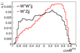
(a)	(b)	(c)

Figure 1: A comparison of the truth level $\cos\theta^{*}$ and the NN output $\cos\theta^{NN}$ distributions for $--$, $++$ and $LL$ events (a), $R_{pT}$ templates for the corresponding polarization states with log scaling (b), and comparison of the $\cos\theta^{NN}$ for the signal and dominant $WZjj$ background (c) are shown with arbitrary units (A.U.). (a) and (c) are the projections of the 2D distributions onto one of the two leptons, which are identical to the projections onto the other lepton due to arbitrary sorting.

Figure 1(a) shows the comparison between the truth $\cos\theta^{*}$ and the NN output $\cos\theta^{NN}$ for $--$, $++$ and $LL$ events ( $+-/L+/L-$ are omitted for clarity, but closely resemble combinations of the templates shown). As expected, $\cos\theta^{NN}$ has less separation power for the different polarization states compared to $\cos\theta^{*}$ due to missing information for the two final state neutrinos. However, reasonable discrimination between each polarization state can clearly be seen from these distributions. Figure 1(b) shows the $R_{pT}$ distribution for $--$, $++$, and $LL$ events. The discrimination power is seen only for large values of $R_{pT}$, and only apparent with a logarithmic scale. Figure 1(c) shows the $\cos\theta^{NN}$ distribution for the signal $W^{\pm}W^{\pm}jj$ process and an important background process: $WZjj$ production. Reasonable separation power is observed, which could be utilized in a combined fit. In an actual data analysis, the $WZjj$ component would be subtracted as background from the observed data before fitting the polarization fractions.

Having established templates for each polarization state and a distribution that is sensitive to different polarization states, we fit the two-dimensional $\cos\theta^{NN}_{1}$ versus $\cos\theta^{NN}_{2}$ distribution in pseudo data to derive each polarization fraction. Five equal-size bins are used for each $\cos\theta^{NN}$ variable ranging from $-1$ to 1. A maximum likelihood fit is performed within the RooFit framework RooFit . We combine events with both $W$ bosons transversely-polarized as “$TT$” (the sum of $--$, $+-$ and $++$ combinations), events with one $W$ boson transversely-polarized and one $W$ boson longitudinally-polarized as “$TL$” (the sum of $L-$ and $L+$ combinations), and events with both $W$ bosons longitudinally-polarized as “$LL$”. This reduces the free fitting parameters from five to two and allows for a better constraint on the $LL$ scattering fraction of interest, under the assumption that the relative admixture of contributions within $TT$ and $TL$ does not change. The two dimensional distributions for these templates are shown in Fig. 2. Statistical fit uncertainties are determined by randomly fluctuating data expectations within their Poisson uncertainties and repeating the fit, and confidence intervals are derived from these toy experiments.

$TT$	$TL$	$LL$

Figure 2: The two dimensional distribution of $\cos\theta^{NN}_{1}$ versus $\cos\theta^{NN}_{2}$ for the two leptons in each event is shown for each of the three polarization states: $TT$, $TL$, and $LL$, respectively.

Fits are performed in a range of integrated luminosities from $0.01-3$ ab^-1. An example fit for 1 ab^-1 is shown in Fig. 3 where the pseudo data are compared to the sum of contributions from $TT$, $TL$ and $LL$ components. It is found that the $LL$ fraction can be measured with a 68% confidence limit of 6.7$\pm 1.4\%$ with an ultimate luminosity of 3 ab^-1. When a similar fit is applied to the $R_{pT}$ variable the precision of 6.7${}^{+7.1}_{-6.7}\%$ is found to be consistent with 0. The regression technique hence greatly enhances the sensitivity to this process.

Figure 3: One example fit where the pseudo data are compared to the sum of contributions from $TT$, $TL$ and $LL$ components. There are five groups with five bins inside each group. These five groups represent $\cos\theta^{NN}_{2}$ from $-1$ to 1 with a step size of 0.4, while five bins inside each group represent $\cos\theta^{NN}_{1}$ from $-1$ to 1 with a step size of 0.4.

The above measurements are performed with parton level predictions. While they show encouraging results it is important to also check if this procedure will stand up to experimental reality of finite detector resolution, and the event level selection that will be required to remove backgrounds from this analysis. To study the effects of event level cuts, we apply additional selection criteria as used by the ATLAS collaboration ATLAS_ssWW to obtain a tighter fiducial region which is dominated by the contribution from electroweak production of $W^{\pm}W^{\pm}jj$ events: jet $p_{T}>30$ GeV, lepton $p_{T}>25$ GeV, missing transverse energy $\not{E}_{T}>40$ GeV, dijet mass $M_{jj}>$500 GeV, and dijet pseudorapidity difference $|\Delta\eta_{jj}|>2.4$.

To emulate the response of a typical general-purpose LHC detector, these events are passed through the application of parton showering in pythiapythia and then through the response simulation of the CMS detector implemented in delphes delphes . This detector smearing adds some degree of realism, but could neglect various effects due to the large number of overlapping interactions during the high luminosity LHC runs. Since these effects are often mitigated with specific reconstruction techniques and need detailed detector modeling, we leave studies of this nature to dedicated efforts by the experiments. After detector simulation, parton level quantities are then approximated by taking the leading two jets clustered with an anti-$k_{t}$ algorithm antikt with jet size parameter R=0.5.

Backgrounds to the $W^{\pm}W^{\pm}jj$ process depend largely on experimental choice, and require detailed simulation. It can be seen in Fig. 1 that background from the $WZjj$ process (where one of the leptons from the $Z$ boson decay is not detected) has a different $\cos\theta^{NN}$ shape than $W^{\pm}W^{\pm}jj$ events, but it is likely event level cuts will still need to be applied to reduce this component. Determining the systematics on the background shapes will require significant work from the experiments, and is not treated here. However, as already mentioned the backgrounds in the $W^{\pm}W^{\pm}jj$ channel are relatively small compared to other channels.

We determine the precision that can be achieved for fractions of $TT$, $TL$, and $LL$ components using three different scenarios increasing in realism: (a) using all generated events at the parton level; (b) using events passing the additional selection criteria used by ATLAS at the parton level; (c) using events processed with the delphes detector simulation and with reconstructed objects passing additional selection criteria used by ATLAS.

The precision for the three polarization fractions as a function of the integrated luminosity is presented in Fig. 4. $TT$ components can be measured with great precision, whereas separating pure $LL$ scattering from $LT$ scattering is challenging. In the most difficult and realistic scenario (c), the cuts and object efficiencies slightly increase the mean $LL$ fraction to 7.0% and 68% confidence limits are found 7${}^{+19}_{-7}$% (7${}^{+5}_{-6}\%$) for an integrated luminosity of 0.1 (3) ab^-1. Equivalent limits from fits to the $R_{pT}$ variable are found to be 7${}^{+29}_{-7}\%$ and 7${}^{+9}_{-7}\%$. The fit to the neural network almost doubles the ultimate precision to anomalous $LL$ fractions in this scenario. Reaching the same statistical sensitivity using the $R_{pT}$ variable would require approximately 10 ab^-1, more than three times the total expected luminosity of the LHC program. We have shown that large sensitivity gains can be made with NN regression. In scenario (c) our simple estimate falls short of the $5\sigma$ criteria for observation of longitudinal VBS, however, new physics beyond the SM could greatly enhance this fraction VLVLBSM , making stringent limits or a future observation of this fraction very important. A comparison of scenarios (a) and (b) to (c) illustrates potential gains in sensitivity through cut optimization and improved detector performance. In addition, the authors hope that experiments can improve on this methodology by training on fully simulated events or by improving detector performance (e.g. through upgrades) to enhance sensitivity.

In conclusion, we present a method to determine the $WW$ polarization fractions in $W^{\pm}W^{\pm}jj$ events by using a deep machine learning technique. This method allows to recover the charged lepton angular distributions in the $W$ boson rest frame from measurable event kinematics. The results obtained from this method show greatly enhanced sensitivity over the example $R_{pT}$ variable. Cuts to reject backgrounds as well as finite detector resolutions reduce the sensitivity as expected, but the method remains a powerful tool for the study of polarization fractions in VBS events, almost doubling the ultimate precision when compared to $R_{pT}$.

We would like to thank our colleagues Sally Dawson, Frank Paige, and Olivier Mattelaer for their help and guidance while preparing this manuscript. The contributions from J.S., L.H. and J.Z. are supported by the U.S. DOE Early Career Grant under contract DE-SC0008062. The work of M.-A.P. is supported by U.S. DOE Contract No. DE-SC0012704. We would also like to acknowledge the role of the U.S. ATLAS Scholar program for fostering collaboration between Michigan and Brookhaven National Laboratory.

Figure 4: 68% (yellow) and 95% (green) expected confidence intervals for the measured $LL$ fraction $f_{LL}$ (top), the $TL$ fraction $f_{TL}$ (middle), and $TT$ fraction $f_{TT}$ (bottom) as a function of the integrated luminosity for, from left to right, scenarios (a),(b), and (c) discussed in the text.

References

- (1) D. A. Dicus, J. F. Gunion, and R. Vega, Phys. Lett. B258 (1991) 475–481.
- (2) M. J. G. Veltman, Acta Phys. Polon. B8 (1977) 475.
- (3) B. W. Lee, C. Quigg, and H. B. Thacker, Phys. Rev. Lett. 38 (1977) 883–885.
- (4) B. W. Lee, C. Quigg, and H. B. Thacker, Phys. Rev. D16 (1977) 1519.
- (5) ATLAS Collaboration, G. Aad et al., Phys.Lett. B716 (2012) 1–29, arXiv:1207.7214 [hep-ex].
- (6) CMS Collaboration, S. Chatrchyan et al., Phys.Lett. B716 (2012) 30–61, arXiv:1207.7235 [hep-ex].
- (7) J. M. Campbell and R. K. Ellis, J. High Energy Phys. 04 (2015) 030, arXiv:1502.02990 [hep-ph].
- (8) A. Alboteanu, W. Kilian, and J. Reuter, J. High Energy Phys. 11 (2008) 010, arXiv:0806.4145 [hep-ph].
- (9) W. Kilian, T. Ohl, J. Reuter, and M. Sekulla, Phys. Rev. D91 (2015) 096007, arXiv:1408.6207 [hep-ph].
- (10) S. Godfrey and K. Moats, Phys. Rev. D81 (2010) 075026, arXiv:1003.3033 [hep-ph].
- (11) C.-W. Chiang, S. Kanemura, and K. Yagyu, Phys. Rev. D90 (2014) 115025, arXiv:1407.5053 [hep-ph].
- (12) ATLAS Collaboration, G. Aad et al., Phys. Rev. Lett. 113 (2014) 141803, arXiv:1405.6241 [hep-ex].
- (13) CMS Collaboration, V. Khachatryan et al., Phys. Rev. Lett. 114 (2015) 051801, arXiv:1410.6315 [hep-ex].
- (14) P. Baldi, P. Sadowski, and D. Whiteson, Nature Commun. 5 (2014) 4308, arXiv:1402.4735 [hep-ph].
- (15) P. Baldi, P. Sadowski, and D. Whiteson, Phys. Rev. Lett. 114 (2015) 111801, arXiv:1410.3469 [hep-ph].
- (16) R. K. Ellis, W. J. Stirling, and B. R. Webber, Camb. Monogr. Part. Phys. Nucl. Phys. Cosmol. 8 (1996) 1–435.
- (17) T. Han, D. Krohn, L.-T. Wang, and W. Zhu, J. High Energy Phys. 03 (2010) 082, arXiv:0911.3656 [hep-ph].
- (18) A. Ballestrero, D. B. Franzosi, and E. Maina, J. High Energy Phys. 06 (2011) 013, arXiv:1011.1514 [hep-ph].
- (19) A. Freitas and J. S. Gainer, Phys. Rev. D D88 (2013) 017302, arXiv:1212.3598.
- (20) K. Doroba, J. Kalinowski, J. Kuczmarski, S. Pokorski, J. Rosiek, et al., Phys.Rev. D86 (2012) 036011, arXiv:1201.2768 [hep-ph].
- (21) M. Fabbrichesi, M. Pinamonti, A. Tonero, and A. Urbano, Phys. Rev. D93 (2016) 015004, arXiv:1509.06378 [hep-ph].
- (22) G. Cybenko, Mathematics of Control, Signals and Systems 2 (1989) 303–314, http://dx.doi.org/10.1007/BF02551274.
- (23) S. Forte, L. Garrido, J. I. Latorre, and A. Piccione, J. High Energy Phys. 05 (2002) 062, arXiv:hep-ph/0204232 [hep-ph].
- (24) P. C. Bhat, Ann. Rev. Nucl. Part. Sci. 61 (2011) 281–309.
- (25) J. Schmidhuber, Neural Networks 61 (2015) 85 – 117, http://www.sciencedirect.com/science/article/pii/S0893608014002135.
- (26) J. Bergstra, O. Breuleux, F. Bastien, P. Lamblin, R. Pascanu, G. Desjardins, J. Turian, D. Warde-Farley, and Y. Bengio in Proceedings of the 9th Python in Science Conference, pp. 3 – 10. 2010.
- (27) F. Bastien, P. Lamblin, R. Pascanu, J. Bergstra, I. J. Goodfellow, A. Bergeron, N. Bouchard, D. Warde-Farley, and Y. Bengio, CoRR abs/1211.5590 (2012) , http://arxiv.org/abs/1211.5590.
- (28) J. Alwall, R. Frederix, S. Frixione, V. Hirschi, F. Maltoni, O. Mattelaer, H. S. Shao, T. Stelzer, P. Torrielli, and M. Zaro, J. High Energy Phys. 07 (2014) 079, arXiv:1405.0301 [hep-ph].
- (29) W. Verkerke and D. P. Kirkby, eConf C0303241 (2003) MOLT007, arXiv:physics/0306116 [physics].
- (30) T. Sjöstrand, S. Mrenna, and P. Z. Skands, Comput. Phys. Commun. 178 (2008) 852–867, arXiv:0710.3820 [hep-ph].
- (31) DELPHES 3 Collaboration, J. de Favereau, C. Delaere, P. Demin, A. Giammanco, V. Lemaître, A. Mertens, and M. Selvaggi, J. High Energy Phys. 02 (2014) 057, arXiv:1307.6346 [hep-ex].
- (32) M. Cacciari, G. P. Salam, and G. Soyez, J. High Energy Phys. 04 (2008) 063, arXiv:0802.1189 [hep-ph].