Improving Ice Sheet Model Calibration Using Paleoclimate and Modern Data

Abstract

Human-induced climate change may cause significant ice volume loss from the West Antarctic Ice Sheet (WAIS). Projections of ice volume change from ice-sheet models and corresponding future sea-level rise have large uncertainties due to poorly constrained input parameters. In most future applications to date, model calibration has utilized only modern or recent (decadal) observations, leaving input parameters that control the long-term behavior of WAIS largely unconstrained. Many paleo-observations are in the form of localized time series, while modern observations are non-Gaussian spatial data; combining information across these types poses non-trivial statistical challenges. Here we introduce a computationally efficient calibration approach that utilizes both modern and paleo-observations to generate better-constrained ice volume projections. Using fast emulators built upon principal component analysis and a reduced dimension calibration model, we can efficiently handle high-dimensional and non-Gaussian data. We apply our calibration approach to the PSU3D-ICE model which can realistically simulate long-term behavior of WAIS. Our results show that using paleo observations in calibration significantly reduces parametric uncertainty, resulting in sharper projections about the future state of WAIS. One benefit of using paleo observations is found to be that unrealistic simulations with overshoots in past ice retreat and projected future regrowth are eliminated.

Keywords: Paleoclimate, West Antarctic Ice Sheet, Computer Model Calibration, Gaussian Process, Dimension Reduction

1 Introduction

Human-induced climate change may cause significant ice volume loss in the polar regions. The West Antarctic Ice Sheet (WAIS) is particularly vulnerable to the changing climate because much of the ice is grounded well below sea level. Previous studies suggest that ice volume loss in this area may result in up to 4 meters of sea level rise (Fretwell et al., 2013), which in turn will require significant resource allocations for adaptation and may therefore have a profound impact on human society (e.g. Lempert et al., 2012).

Many recent modeling efforts have focused on simulating and projecting the past and future WAIS volume dynamics (e.g Bindschadler et al., 2013). The relevant time scale for many aspects of WAIS behavior is often in hundreds to thousands of years; this in turn necessitates simulating and projecting the evolution of WAIS for a very long time span (Cornford et al., 2015; Feldmann and Levermann, 2015; Golledge et al., 2015; Gomez et al., 2015; Ritz et al., 2015; Winkelmann et al., 2015).

In this work we use the PSU3D-ICE model (Pollard and DeConto, 2009, 2012b, 2012a) to simulate the long-term evolution of the West Antarctic Ice Sheet. Using a hybrid dynamical core that combines the shallow-ice and the shallow-shelf approximation, the model can realistically simulate the long-term behavior of the ice sheet with reasonable amount of computational effort. In contrast to higher-resolution models (e.g. Gladstone et al., 2012; Favier et al., 2014; Joughin et al., 2014) that are designed for relatively short simulations with more detailed physical processes, this modeling strategy enables us to simulate the long-term evolution of the West Antarctic Ice Sheet and utilize information from paleo-observations for model calibration. The approach here is a tradeoff between (i) reduced fidelity in capturing details such as sills near modern grounding lines that may be important for 10’s-km scale retreat in the next hundred years, and (ii) more robust calibration versus retreat over hundreds of kilometres and more pronounced bedrock variations, which is arguably more relevant to larger-scale retreat into the West Antarctic interior within the next several centuries.

Parametric uncertainty is an important source of uncertainty in projecting future WAIS volume change. Ice sheet models have input parameters that strongly affect the model behaviors; they are also poorly constrained (Stone et al., 2010; Applegate et al., 2012). Various calibration methods have been proposed to reduce parametric uncertainty for Greenland (Chang et al., 2014a; McNeall et al., 2013) and the Antarctica ice sheets model (Gladstone et al., 2012; Chang et al., 2015). Although these recent studies have provided statistically sound ways of generating constrained future projections, they are mostly limited to generating short-term projections (i.e. a few hundred years from present) or utilizing modern or recent observations in the calibration. Inferring input parameters that are related to the long-term behavior of WAIS is crucial for generating well constrained projections in the relevant time scale (hundreds to thousands of years). Modern or recent observations often lack information on these parameters and therefore calibrating solely based on these information sources may result in poorly-constrained projections. Recent studies using heuristic approaches suggest that utilizing information from paleo data can reduce uncertainties in these long-term behavior related parameters (Whitehouse et al., 2012b, a; Briggs et al., 2013; Briggs and Tarasov, 2013; Briggs et al., 2014; Golledge et al., 2014; Maris et al., 2015).

Here we propose an approach to simultaneously utilizing modern- and paleo-observations for ice sheet model calibration, generating well-constrained future WAIS ice volume change projections. This work represents the first statistically rigorous approach for calibrating an ice sheet model based on both modern and paleo data, and the resulting inference about parameters and projected sea level rise are therefore less uncertain than those obtained solely based on modern data (cf. Chang et al., 2015). Our methodological contribution is to provide a computationally expedient approach to fuse information from modern and paleo data. Our dimension reduction methods build upon two different calibration approaches given by Chang et al. (2014b) and Chang et al. (2015), while also accounting for potential relationships between the two very different types of data – the modern data are spatial and binary while the paleo data are in the form of a time series. A central contribution of this work is scientific. Based on our methods, we are able to show explicitly how paleo data provides key new information about parameters of the ice sheet model, and we thereby show that utilizing paleo data in addition to modern ice sheet data virtually eliminates the possibility of zero (or negative) sea level rise.

The rest of the paper is organized as follows. Section 2 introduces the model runs and the observational data sets used in our calibration experiment. Section 3 explains our computationally efficient reduced-dimension calibration approach that enables us to emulate and calibrate the PSU3D-ICE model using both the grounding line positions and the modern observations while avoiding the computational and inferential challenges. Section 4 describes our calibration experiment results based on a simulated example and real observations. Finally, in Section 5, we summarize our findings and discuss caveats and possible improvements.

2 Model Runs and Observational Data

In this section, we describe the ice-sheet model that we use to simulate past and future West Antarctic Ice Sheet behavior, as well as the modern and paleo-data sets that we use to calibrate the ice-sheet model.

2.1 Model Runs and Input Parameter Decription

We calibrate the following four model parameters that are considered to be important in determining the long-term evolution of the West Antarctic Ice Sheet, yet whose values are particularly uncertain: the sub-ice-shelf oceanic melt factor (OCFAC), the calving factor (CALV), the basal sliding coefficient (CRH), and the asthenospheric relaxation e-folding time (TAU). OCFAC (non-dimensional) represents the strength of oceanic melting at the base of floating ice shelves in response to changing ocean temperatures, and CALV (non-dimensional) determines the rate of iceberg calving at the outer edges of floating ice shelves. CRH (m year^-1 Pa^-2) represents how slippery the bedrock is in areas around Antarctica that are currently under ocean, i.e., how fast grounded ice slides over these areas as it expands beyond the present extent. A higher value of CRH corresponds to faster basal sliding and greater ice flux towards the ocean. TAU (with units in thousands of years) represents the time scale for vertical bedrock displacements in response to changing ice load. In this paper, we remap the parameter values to the $[0,1]$ intervals for convenience. We refer to Chang et al. (2015) for more detailed description of these parameters.

We run the PSU3D-ICE model with 625 different parameter settings specified by a factorial design, with five different values for each parameter. Starting from 40,000 years before present, each model run is spun up until present and then projected 5,000 years into the future. For atmospheric forcing, we use the modern climatological Antarctic dataset from the Sea Rise project (Bindschadler et al., 2013) uniformly perturbed in proportion to a deep-sea-core d18O record (Pollard and DeConto, 2009, 2012a). For oceanic forcing, we use the ocean temperature pattern from AOGCM simulation runs generated by Liu et al. (2009). From each model run we extract the following two data sets and compare them to the corresponding observational record: (i) the time series of grounding line positions, the location of the transition from grounded ice to ice shelf along the central flowline in the the Amundsen Sea Embayment (ASE) region (see Section 2.2 below for more details), and (ii) the modern binary spatial pattern of presence and absence of grounded ice in the ASE. The grounding line position time series (i) has 1,501 time points from 15,000 years ago to the present, and the modern binary spatial pattern (ii) is a binary map with $86\times 37$ pixels with a 20 km horizontal resolution. Because the time series of the grounding line position for each model run does not usually show much change until 15,000 years before present, we only use the time series after 15,000 years ago for our calibration. Note that each model output is in the form of high-dimensional multivariate data, which causes computational and inferential challenges described in Section 3.1.4. The corresponding observational data sets, described below, have the same dimensionalities as the model output sets.

Note that, for some parameter settings, the past grounding line position shows unrealistically rapid retreat early in the time series and does not change for the rest of the time period. We have found that using these runs for building our emulator negatively affects the emulation performance for more realistic model outputs. Therefore, we have exclude the model runs that reach a grounding line position 500 meters inland from the modern grounding line before 10,000 years ago from our analysis and use the remaining 461 model runs for emulating the past grounding line position output.

2.2 Paleo-records of Grounding Line Positions

We take advantage of a very recent, comprehensive synthesis of Antarctic grounding-line data since the last glacial maximum (RAISED Consortium, 2014). For the ASE sector, Larter et al. (2014) provide spatial maps of estimated grounding lines at 5,000 year intervals from 25,000 years ago to the present. These maps are based primarily on many ship-based observations taken in the oceanic part of ASE using sonar (showing patterns of ocean-floor features formed by flow of past grounded ice) and shallow sediment cores (providing dating and information on ice proximity, i.e., open ocean, ice proximal or grounded). There is considerable uncertainty in the reconstructions, but general consensus for the overall retreat in this sector, especially along the central flowline of the major paleo-ice stream emerging from the confluence of Pine Island and Thwaites Glaciers and crossing the ASE (cf. earlier synthesis by Kirshner et al., 2012).

2.3 Modern Observations

We use a map of modern grounding lines deduced from the Bedmap2 dataset (Fretwell et al., 2013). Bedmap2 is the most recent all-Antarctic dataset that provides gridded maps of ice surface elevation, bedrock elevation, and ice thickness. These fields were derived from a variety of sources, including satellite altimetry, airborne and ground radar surveys, and seismic sounding. The nominal Bedmap2 grid spacing is 1 km, but the actual coverage in some areas is sparser especially for ice thickness. We deduce grounding line locations by a simple floatation criterion at each model grid cell, after interpolating the data to our coarser model grid. In this work, we use a part of the data that corresponds to the ASE sector, which is expected to be the largest contributor to future sea level rise caused by WAIS volume loss (Pritchard et al., 2012). Since the observed modern binary pattern is derived from the highly accurate ice thickness measurements in the Bedmap2 data set and the model binary patterns are highly variable depending on the input parameter settings (see Section S1 and Figure S1 in the Supplement), the model outputs approximated by our emulator are accurate enough to provide a basis for calibration.

3 Computer Model Emulation and Calibration Using Dimension Reduction

As explained in the preceding discussion, parameter inference is central to WAIS volume change projections; taking full advantage of all observational data, both paleo and modern, may result in reduced parametric uncertainty which in turn can result in well-constrained projections of volume change. In this section we describe our statistical approach for inferring input parameters for WAIS models while accounting for relevant sources of uncertainty. In Section 3.1 we introduce our two-stage framework (Bayarri et al., 2007; Bhat et al., 2010, 2012; Chang et al., 2014b) that consists of the emulation and the calibration steps: In the emulation step we build a Gaussian process emulator as a fast approximation to WAIS model outputs (Sacks et al., 1989). In the calibration step, we infer the input parameters for WAIS models by combining information from emulator output and observational data while accounting for the systematic model-observation discrepancy. The framework faces computational and inferential challenges when model output and observational data are high-dimensional data such as large spatial patterns or long time series, and the challenges are further exacerbated when the marginal distribution of model output and observational data cannot be modeled by a Gaussian distribution. Section 3.2 describes a computationally expedient reduced-dimension approach that mitigates these challenges for high-dimensional Gaussian and non-Gaussian data and enables us to utilize information from both past grounding line positions and modern binary patterns for calibration.

We use the following notation henceforth: Let $\boldsymbol{\theta}_{1},\dots,\boldsymbol{\theta}_{q}\in R^{4}$ be the parameter settings at which we use both the past grounding line positions and the modern binary patterns for emulation and $\boldsymbol{\theta}_{q+1},\dots,\boldsymbol{\theta}_{p}\in R^{4}$ be the settings at which we use only the the modern binary patterns (see Section 2.1 above for the reason why $q$ is less than $p$ in our experiment). We denote the past grounding line position time series from our WAIS model at a parameter setting $\boldsymbol{\theta}$ and a time point $t$ by $Y_{1}(\boldsymbol{\theta},t)$. We let $\mathbf{Y}_{1}$ be a $q\times n$ matrix where its $i$th row is $[Y_{1}(\boldsymbol{\theta}_{i},t_{1}),\dots,Y_{1}(\boldsymbol{\theta}_{i},t_{n})]$ and $t_{1},\dots,t_{n}$ are time points at which the grounding line positions are recorded. We let $\mathbf{Z}_{1}=[Z_{1}(t_{1}),\dots,Z_{1}(t_{n})]$ be a vector of the observed time series of past grounding line positions reconstructed from paleo records. Similarly, we denote the modern ice-no ice binary output at the parameter setting $\boldsymbol{\theta}$ and a spatial location $\mathbf{s}$ by $Y_{2}(\boldsymbol{\theta},\mathbf{s})$. We let $\mathbf{Y}_{2}$ be a $p\times m$ matrix where its $i$th row is $[Y_{2}(\boldsymbol{\theta}_{i},\mathbf{s}_{1}),\dots,Y_{2}(\boldsymbol{\theta}_{i},\mathbf{s}_{m})]$ with model grid points $\mathbf{s}_{1},\dots,\mathbf{s}_{m}$. The corresponding observational data are denoted by an $m$-dimensional vector $\mathbf{Z}_{2}=[Z_{2}(\mathbf{s}_{1}),\dots,Z_{2}(\mathbf{s}_{m})]$. For our WAIS model emulation and calibration problem in Section 4, $n=1,501$, $m=3,182$, $p=625$, and $q=461$.

3.1 Basic WAIS Model Emulation and Calibration Framework

In this subsection we explain the basic general framework for computer model emulation and calibration and describe the computational challenges posed by our use of high-dimensional model output and observational data.

3.1.1 Emulation and Calibration using Past Grounding Line Positions

We start with the model output $\mathbf{Y}_{1}$ and the observational data $\mathbf{Z}_{1}$ for the past grounding line positions. Since computer model runs are available only at a limited number of parameter settings $q$, one needs to construct a statistical model for approximating the model output at a new parameter setting $\boldsymbol{\theta}$ by interpolating the existing model output obtained at the design points $\boldsymbol{\theta}_{1},\dots,\boldsymbol{\theta}_{q}$ (Sacks et al., 1989). Constructing this statistical model requires us to build a Gaussian process that gives the following probability model for the existing $q$ model runs with $n$-dimensional output:

$$\mbox{vec}\left(\mathbf{Y}_{1}\right)\sim N(\mathbf{X}_{1}\boldsymbol{\beta}_{1},\boldsymbol{\Sigma}(\boldsymbol{\xi}_{1})),$$ (1)

where $\mbox{vec}(.)$ is the vectorization operator that stacks the columns of a matrix into one column vector, and $\mathbf{X}_{1}$ is a $nq\times b$ covariate matrix that contains all the time coordinates and the input parameters settings used in the $nq\times nq$ covariance matrix $\boldsymbol{\Sigma}(\boldsymbol{\xi}_{1})$ with a covariance parameter vector $\boldsymbol{\xi}_{1}$. The $b$-dimensional vector $\boldsymbol{\beta}_{1}$ contains all the coefficients for the columns of $\mathbf{X}_{1}$. When the number of time points $n$ and the number of parameter settings $q$ are small, one can estimate the parameter $\boldsymbol{\xi}_{1}$ by maximizing the likelihood function corresponding to the probability model in (1) and finding the conditional distribution of $Y_{1}(\boldsymbol{\theta}_{i},t_{1}),\dots,Y_{1}(\boldsymbol{\theta}_{i},t_{n})$ given $\mathbf{Y}_{1}$ for any new value of $\boldsymbol{\theta}$ using the fitted Gaussian process with the maximum likelihood estimates $\hat{\boldsymbol{\beta}}_{1}$ and $\hat{\boldsymbol{\xi}}_{1}$. We call the fitted Gaussian process an emulator and denote the output at $\boldsymbol{\theta}$ interpolated by the emulator as $\boldsymbol{\eta}(\boldsymbol{\theta},\mathbf{Y}_{1})$. Using the emulator, one can set up a model for inferring the input parameter $\boldsymbol{\theta}$ as follows (Kennedy and O’Hagan, 2001; Bayarri et al., 2007):

$$\mathbf{Z}_{1}=\boldsymbol{\eta}(\boldsymbol{\theta},\mathbf{Y}_{1})+\boldsymbol{\delta},$$ (2)

where $\boldsymbol{\delta}$ is an $n$-dimensional random vector that represents model-observation discrepancy. The discrepancy term $\boldsymbol{\delta}$ is often modeled by a Gaussian process that is independent of the emulated output $\boldsymbol{\eta}(\boldsymbol{\theta},\mathbf{Y}_{1})$. Using a posterior density defined by the likelihood function that corresponds to the probability model in (2) and a standard prior specification, one can estimate the input parameter $\boldsymbol{\theta}$ along with other parameters in the model via Markov Chain Monte Carlo (MCMC).

3.1.2 Emulation and Calibration using Modern Binary Observations

Emulation and calibration for the modern ice-no ice binary patterns require additional consideration in model specification due to the binary nature of the data sets. Inspired by the generalized linear model framework, Chang et al. (2015) specifies emulation and calibration models in terms of logits of model output and observational data. Let $\boldsymbol{\Gamma}=\left\{\gamma_{ij}\right\}$ be a $p\times m$-dimensional matrix whose element is the logit of the $(i,j)$th element in $\mathbf{Y}_{2}$, i.e.,

$$P(Y_{2}(\boldsymbol{\theta}_{i},\mathbf{s}_{j})=y_{ij})= \left(\frac{\exp(\gamma_{ij})}{1+\exp(\gamma_{ij})}\right)^{y_{ij}}\left(\frac{1}{1+\exp(\gamma_{ij})}\right)^{1-y_{ij}}$$

$$= (1+\exp(-(2y_{ij}-1)\gamma_{ij}))^{-1},$$

where the value of $y_{ij}$ is ether 0 or 1. Assuming conditional independence between the elements in $\mathbf{Y}_{2}$ given $\boldsymbol{\Gamma}$, one can use a Gaussian process that yields the probability model below to specify the dependence between the model output at different parameter settings and spatial locations,

$$\mbox{vec}\left(\boldsymbol{\Gamma}\right)\sim N(\mathbf{X}_{2}\boldsymbol{\beta}_{2},\boldsymbol{\Sigma}(\boldsymbol{\xi}_{2})),$$ (3)

where the $mp\times c$ dimensional covariate matrix $\mathbf{X}_{2}$, $c$-dimensional coefficient vector $\boldsymbol{\beta}_{2}$, and the $mp\times mp$ covariance matrix $\boldsymbol{\Sigma}(\boldsymbol{\xi}_{2})$ with a covariance parameter vector $\boldsymbol{\xi}_{2}$ are defined in the same way as in (1). One can find the maximum likelihood estimates $\hat{\boldsymbol{\beta}}_{2}$ and $\hat{\boldsymbol{\xi}}_{2}$ by maximizing the likelihood function corresponding to the probability model in (3). The resulting Gaussian process emulator gives a vector of interpolated logits $\boldsymbol{\psi}(\boldsymbol{\theta},\mathbf{Y}_{2})$ for a new input parameter value $\boldsymbol{\theta}$.

The calibration model is also defined in terms of the logits of the observational data $\mathbf{Z}_{2}$, denoted by an $m$-dimensional vector $\boldsymbol{\lambda}=[\lambda_{1},\dots,\lambda_{m}]$,

$$\boldsymbol{\lambda}=\boldsymbol{\psi}(\boldsymbol{\theta},\mathbf{Y}_{2})+\boldsymbol{\phi},$$

where $\boldsymbol{\phi}$ is an $m$-dimensional random vector representing the model-observation discrepancy defined in terms of the logits of $\mathbf{Z}_{2}$. Again, assuming conditional independence between the elements in $\mathbf{Z}_{2}$ given $\boldsymbol{\lambda}$, the relationship between $\boldsymbol{\lambda}$ and $Z_{2}(\mathbf{s}_{i})$ is given by

$$\begin{split}P(Z_{2}(\mathbf{s}_{j})=z_{j})=&\left(\frac{\exp(\lambda_{j})}{1+\exp(\lambda_{j})}\right)^{z_{j}}\left(\frac{1}{1+\exp(\lambda_{i})}\right)^{1-z_{j}}\\ =&(1+\exp(-(2z_{j}-1)\lambda_{j}))^{-1},\end{split}$$ (4)

where $z_{j}$ takes a value of either 0 or 1. If the number of parameter settings $p$ and spatial locations $m$ are small, one can set up a posterior density based on the likelihood function corresponding to the probability models above and some standard prior specifications and might be able to infer $\boldsymbol{\theta}$ and other parameters using MCMC.

3.1.3 Combining Information from Two Data Sets in Calibration

We set up a calibration model to infer the input parameters in $\boldsymbol{\theta}$ based on the models described in Sections 3.1.1 and 3.1.2. The main consideration here is how to model the dependence between $\mathbf{Z}_{1}$ and $\mathbf{Z}_{2}$, which can be translated to the dependence between the emulated outputs $\boldsymbol{\eta}(\boldsymbol{\theta},\mathbf{Y}_{1})$ and $\boldsymbol{\psi}(\boldsymbol{\theta},\mathbf{Y}_{2})$ and the dependence between the discrepancy terms $\boldsymbol{\delta}$ and $\boldsymbol{\phi}$. We model the dependence between $\boldsymbol{\eta}(\boldsymbol{\theta},\mathbf{Y}_{1})$ and $\boldsymbol{\psi}(\boldsymbol{\theta},\mathbf{Y}_{2})$ only through the input parameter $\boldsymbol{\theta}$ (i.e., we assume that $\boldsymbol{\eta}(\boldsymbol{\theta},\mathbf{Y}_{1})$ and $\boldsymbol{\psi}(\boldsymbol{\theta},\mathbf{Y}_{2})$ are conditionally independent given the input parameter $\boldsymbol{\theta}$), because the emulators are independently constructed for $\mathbf{Y}_{1}$ and $\mathbf{Y}_{2}$. We do not introduce a conditional dependence between the emulators $\boldsymbol{\eta}(\boldsymbol{\theta},\mathbf{Y}_{1})$ and $\boldsymbol{\psi}(\boldsymbol{\theta},\mathbf{Y}_{2})$ given $\boldsymbol{\theta}$ because the emulators are already highly accurate. The greater challenge is the dependence between the discrepancy terms $\boldsymbol{\delta}$ and $\boldsymbol{\phi}$ because both terms are high-dimensional and it is not straightforward to find a parsimonious model that can efficiently handle the cross-correlation between them (see Section 3.1.4 below for further discussion and Section 3.2 for our solution).

3.1.4 Computational and Inferential Challenges

The emulation and calibration problems for both the past grounding line positions and the modern ice-no ice binary patterns face computational and inferential challenges when the length of time series $n$ and the number of spatial locations $m$ are large. For both of these problems, the likelihood evaluation in the emulation step involves Cholesky decomposition of $nq\times nq$ and $mp\times mp$ covariance matrices, which scales as $\mathcal{O}(n^{3}q^{3})$ and $\mathcal{O}(m^{3}p^{3})$ respectively. For our WAIS model calibration problem, this requires $\frac{1}{3}n^{3}q^{3}=1.1\times 10^{17}$ and $\frac{1}{3}m^{3}p^{3}=2.6\times 10^{18}$ flops of computation for each likelihood evaluation, which translate to about 28,000 hours and 220,000 hours on a high-performance single core. Moreover, emulation and calibration using the modern ice-no ice patterns poses additional inferential difficulties. In particular, we need to compute $mp=1,988,750$ logits for the model output in the emulation step and $2m=6,364$ logits for the observational data. The challenge is therefore to ensure that the problem is well-posed by constraining the logits, while at the same time retaining enough flexibility in the model. The problem is even more complicated due to the dependence between the discrepancy terms $\boldsymbol{\delta}$ and $\boldsymbol{\phi}$, because we need to estimate $n\times m=1,501\times 3,182$ correlation coefficients between the elements in those two terms.

3.2 Reduced-dimension Approach

In this subsection, we discuss our reduced-dimension approaches to mitigate the computational and inferential challenges described above.

3.2.1 Dimension Reduction using Principal Components

The first step is to reduce the dimensionality of model output via principal component analysis. For the model output matrix of the past grounding line positions $\mathbf{Y}_{1}$ we find the $J_{1}$-leading principal components by treating each of its columns (i.e. output for each time point) as different variables and rows (i.e. output for each parameter setting) as repeated observations. For computational convenience we rescale the principal component scores by dividing them by the square roots of their corresponding eigenvalues so that their sample variances become 1. We denote the $j$th rescaled principal component scores at the parameter setting $\boldsymbol{\theta}$ as $Y_{1}^{R}(\boldsymbol{\theta},j)$ and the $q\times J_{1}$ matrix that contains all the principal component scores for the design points $\boldsymbol{\theta}_{1},\dots,\boldsymbol{\theta}_{q}$ as $\mathbf{Y}_{1}^{R}=\left\{Y_{1}^{R}(\boldsymbol{\theta}_{i},j)\right\}$ with its rows for different parameter settings and columns for different principal components. Similarly, for the model output matrix of the modern ice-no ice binary patterns patterns $\mathbf{Y}_{2}$ we form a $p\times J_{2}$ matrix $\mathbf{Y}_{2}^{R}=\left\{Y_{2}^{R}(\boldsymbol{\theta}_{i},j)\right\}$ of $J_{2}$ leading logistic principal components in the same way, where $Y_{2}^{R}(\boldsymbol{\theta},j)$ is the $j$th logistic principal component at the parameter setting $\boldsymbol{\theta}$.

We use $J_{1}=20$ principal components for the past grounding position output and $J_{2}=10$ for the modern binary pattern output. Through a cross validation experiment described below in Section 4, we have found that increasing the number of principal components does not improve the emulation performance. We have also confirmed that the principal component score surfaces vary smoothly in the parameter space and hence Gaussian process emulation is a suitable approach to approximating them (Figures S2-S7 in the Supplement).

We display the first three principal components for modern binary spatial pattern in Figure S8 and past grounding line position time series in Figure S9. The first three principal components for the modern binary spatial pattern show that the most variable patterns between parameter settings are (i) the overall ice coverage in the inner part of the Amundsen Embayment, which determines whether there is a total collapse of ice sheet in this area, (ii) the grounding line pattern around the edge of Amundsen Sea Embayment, (iii) and the ice coverage around the Thurston island. The first three principal components for the past grounding line position time series indicate that the most variable patterns between the input parameter settings are (i) the grounding-line retreat occurring between 15,000 and 7,000 years ago, (ii) retreat occurring until around 9,000 years ago, followed by strong re-advance until 3,000 years ago (red dashed curve), and (iii) a quasi-sinusoidal advance and retreat (black dashed-dotted curve) that spans the entire time period.

3.2.2 Emulation using Principal Components

In the emulation step, our principal component-based approach allows us to circumvent expensive matrix computations in likelihood evaluation (Section 3.1.4, above) by constructing emulators for each principal component separately. For the $j$th principal component of $\mathbf{Y}_{1}$, we fit a Gaussian process model to $Y_{1}^{R}(\boldsymbol{\theta}_{1},j),\dots,\allowbreak Y_{1}^{R}(\boldsymbol{\theta}_{q},j)$ ($j=1,\dots,J_{1}$) with 0 mean and the following covariance function:

$$\mbox{Cov}(Y_{1}^{R}(\boldsymbol{\theta}_{k},j),Y_{1}^{R}(\boldsymbol{\theta}_{l},j))=\kappa_{1,j}\exp\left(-\sum_{i=1}^{4}\frac{|\theta_{ik}-\theta_{il}|}{\phi_{1,ij}}\right)+\zeta_{1,j}1(\boldsymbol{\theta}_{k}=\boldsymbol{\theta}_{l}),$$

with $\kappa_{1,j},\phi_{1,1j},\dots,\phi_{1,4j},\zeta_{1,j}>0$ by finding the MLEs $\hat{\kappa}_{1,j},\hat{\phi}_{1,1j},\dots,\hat{\phi}_{1,4j}$, and $\hat{\zeta}_{1,j}$. The computational cost for likelihood evaluation is reduced from $\mathcal{O}\left(q^{3}n_{1}^{3}\right)$ to $\mathcal{O}\left(J_{1}q^{3}\right)$. The resulting $J_{1}$ Gaussian process models allow us to interpolate the values of the principal components at any new value of $\boldsymbol{\theta}$. We denote the collection of the predicted values given by these Gaussian process models for parameter setting $\boldsymbol{\theta}$ as $\boldsymbol{\eta}(\boldsymbol{\theta},\mathbf{Y}_{1}^{R})$. Similarly we construct Gaussian process models for the logistic principal components $Y_{2}^{R}(\boldsymbol{\theta}_{1},j),\dots,Y_{2}^{R}(\boldsymbol{\theta}_{p},j)$ ($j=1,\dots,J_{2}$) with mean 0 and the covariance function

$$\mbox{Cov}(Y_{2}^{R}(\boldsymbol{\theta}_{k},j),Y_{2}^{R}(\boldsymbol{\theta}_{l},j))=\kappa_{2,j}\exp\left(-\sum_{i=1}^{4}\frac{|\theta_{ik}-\theta_{il}|}{\phi_{2,ij}}\right)+\zeta_{2,j}1(\boldsymbol{\theta}_{k}=\boldsymbol{\theta}_{l}),$$

with $\kappa_{2,j},\phi_{2,1j},\dots,\phi_{2,4j},\zeta_{2,j}>0$, by finding the MLEs $\hat{\kappa}_{2,j},\hat{\phi}_{2,1j},\dots,\hat{\phi}_{2,4j}$, and $\hat{\zeta}_{2,j}$. This reduces the computational cost for likelihood evaluation from $\mathcal{O}(m^{3}p^{3})$ to $\mathcal{O}(J_{2}p^{3})$. Moreover, our approach requires computing only $p\times J_{2}$ logistic principal components and hence eliminates the need for computing $mp$ logits. As above, we let $\boldsymbol{\psi}(\boldsymbol{\theta},\mathbf{Y}_{2}^{R})$ be the collection of the values of logistic principal components at any new value of $\boldsymbol{\theta}$ interpolated by the Gaussian process models.

3.2.3 Dimension-reduced Calibration

In the calibration step, we use basis representations for the observational data sets using the emulators for the principal components constructed above to mitigate the computational and inferential challenges explained in Section 3.1.4. For the observed past grounding line positions $\mathbf{Z}_{1}$ we set up the following linear model:

$$\mathbf{Z}_{1}=\mathbf{K}_{1,y}\boldsymbol{\eta}(\boldsymbol{\theta},\mathbf{Y}_{1}^{R})+\mathbf{K}_{1,d}\boldsymbol{\nu}_{1}+\boldsymbol{\epsilon}_{1},$$ (5)

where $\mathbf{K}_{1,y}$ is the $n\times J_{1}$ matrix for the eigenvectors for the leading principal components rescaled by square roots of their corresponding eigenvalues, $\mathbf{K}_{1,d}\boldsymbol{\nu}_{1}$ is a low-rank representation of the discrepancy term $\boldsymbol{\delta}$, with an $n\times M$ basis matrix $\mathbf{K}_{1,d}$ and its $M$-dimensional random coefficient vector $\boldsymbol{\nu}_{1}\sim N(\mathbf{0},\alpha_{1}^{2}\mathbf{I}_{M})$ $(\alpha_{1}^{2}>0)$, and $\boldsymbol{\epsilon}_{1}$ is a vector of $n$ i.i.d random errors with mean 0 and variance $\sigma_{\epsilon}^{2}>0$ (see Section 3.3 below for the details on specifying $\mathbf{K}_{1,d}$). Inferring parameters using dimension-reduced observational data computed based on the representation in (5) leads to a significant computational advantage by reducing the computational cost for likelihood evaluation from the order of $\mathcal{O}(n^{3})$ to the order of $\mathcal{O}\left((J_{1}+M)^{3}\right)$ (see Appendix A for details).

The idea of using principal components and kernel convolution in calibration is similar to the approach described in Higdon et al. (2008). However, our approach enables a faster computation by emulating each principal component separately and formulating the calibration model in terms of the dimension-reduced observational data $\mathbf{Z}_{1}^{R}$; the approach in Higdon et al. (2008) retains the original data $\mathbf{Z}_{1}$ and hence their computational gains are primarily due to more efficient matrix operations. Moreover, we use a two stage approach (cf. Bayarri et al., 2007; Bhat et al., 2012; Chang et al., 2014b), which separates the emulation and the calibration steps, to reduce the identifiability issues between the parameters in the emulator and the discrepancy term.

For the modern observed ice-no ice binary patterns $\mathbf{Z}_{2}$ we set up the following linear model for the logits:

$$\boldsymbol{\lambda}=\mathbf{K}_{2,y}\boldsymbol{\psi}(\boldsymbol{\theta},\mathbf{Y}_{2}^{R})+\mathbf{K}_{2,d}\boldsymbol{\nu}_{2},$$ (6)

where $\mathbf{K}_{2,y}$ is the $m\times J_{2}$ eigenvectors for the leading logistic principal components and $\mathbf{K}_{2,d}$ is an $m\times L$ basis matrix with $L$-dimensional random coefficients $\boldsymbol{\nu}_{2}\sim N(\mathbf{0},\alpha_{2}^{2}\mathbf{I}_{L})$ (see Section 3.3 below for the details on specifying $\mathbf{K}_{2,d}$). This basis representation also reduces the cost for matrix computation from $\mathcal{O}(m^{3})$ to $\mathcal{O}(J_{2}p^{3})$. More importantly, using this basis representation reduces the number of logits that need to be estimated from $2m$ to $J_{2}+L$, and hence makes the calibration problem well-posed. Using the model in (5) and (6) and additional prior specification we can set up the posterior density and estimate the input parameters $\boldsymbol{\theta}$ while accounting for the uncertainty in other parameters via MCMC using the standard Metropolis-Hastings algorithm. We describe posterior density specification in more details in Appendix B.

We need to consider the dependence between $\mathbf{Z}_{1}$ and $\mathbf{Z}_{2}$ to use the information from both data sets simultaneously. As discussed above we model the dependence between the emulators through the input parameter $\boldsymbol{\theta}$. We also capture the dependence between the discrepancy terms through the $M\times L$ cross correlation matrix $\mathbf{R}_{\nu}$ between $\boldsymbol{\nu}_{1}$ and $\boldsymbol{\nu}_{2}$, where the $(i,j)$th element of $\mathbf{R}_{\nu}$ is $\rho_{\nu,ij}=\mbox{Cov}(\nu_{1i},\nu_{2j})$ and $\nu_{1i}$ and $\nu_{2j}$ are respectively the $i$th and $j$th elements of $\boldsymbol{\nu}_{1}$ and $\boldsymbol{\nu}_{2}$ (See Appendix A and B for further details). This greatly reduces the inferential issue by reducing the number of cross-correlation coefficients that need to be estimated from $mn$ to $ML$.

3.3 Model-Observation Discrepancy

For a successful computer model calibration it is important to find good discrepancy basis matrices $\mathbf{K}_{1,d}$ and $\mathbf{K}_{2,d}$ that allow enough flexibility in representing the model-observation discrepancies while avoiding identifiability issues in estimating $\boldsymbol{\theta}$ (cf. Brynjarsdóttir and O’Hagan, 2014). To define the discrepancy basis matrix for the past grounding line positions $\mathbf{K}_{1,d}$ we use a kernel convolution approach using $M<n$ knot points $a_{1},\dots,a_{M}$ that are evenly distributed between $t_{1}$ and $t_{n}$. We use the following exponential kernel function to define the correlation between $t_{1},\dots,t_{n}$ and $a_{1},\dots,a_{M}$:

$$\left\{\mathbf{K}_{1,d}\right\}_{ij}=\exp\left(-\frac{\left|t_{i}-a_{j}\right|}{\phi_{1,d}}\right),$$ (7)

with a fixed value $\phi_{1,d}>0$. The basis representation based on this kernel function enables us to represent the general trend in model-observation discrepancy using a small number of random variables for the knot locations. Note that the discrepancy term constructed by kernel convolution can confound the effect from model parameters and thus cause identifiability issues; any trend produced by $\mathbf{K}_{1,y}\boldsymbol{\eta}(\boldsymbol{\theta},\mathbf{Y}_{1}^{R})$ can be easily approximated by $\mathbf{K}_{1,d}\boldsymbol{\nu}_{1}$ and therefore one cannot distinguish the effects from these two terms (Chang et al., 2014b). To avoid this issue, we replace $\mathbf{K}_{1,d}$ with its leading eigenvectors, which corresponds to regularization given by ridge regression (see Hastie et al., 2009, pg. 66). In the calibration experiment in Section 4 we chose the value of $\phi_{1,d}$ as 750 (years), the number of knots as $M=1,500$, and the the number of eigenvectors as 300 and confirmed that using the discrepancy term based on these values leads to a reasonable calibration result by a simulated example (Section 4.1). We have also found that different settings for these values lead to similar calibration results and hence inference for $\boldsymbol{\theta}$ is robust to choice of these values (cf. Chang et al., 2014b).

The identifiability issue explained above is further complicated for the modern ice-no ice binary patterns because binary patterns provide even less information for separating the effects from the input parameters and the discrepancy term than continuous ones do. Through some preliminary experiments (not shown here) we found that the regularization introduced above does not solve the identifiability issue for binary patterns. Therefore we use an alternative approach to construct the discrepancy basis $\mathbf{K}_{2,d}$, which is based on comparison between model runs and observational data (Chang et al., 2015). In this approach $\mathbf{K}_{2,d}$ has only one column (i.e. $L=1$) and therefore the matrix is reduced to a column vector $\mathbf{k}_{2,d}$ and its coefficient vector $\boldsymbol{\nu}_{2}$ becomes a scalar $\nu_{2}$. For the $j$th location $\mathbf{s}_{j}$ we calculate the following signed mismatch between the model and observed binary outcomes:

$$r_{j}=\frac{1}{p}\sum_{i=1}^{p}\mbox{sgn}(Y_{2}(\boldsymbol{\theta}_{i},\mathbf{s}_{j})-Z_{2}(\mathbf{s}_{j}))I(Y_{2}(\boldsymbol{\theta}_{i},\mathbf{s}_{j})\neq Z_{2}(\mathbf{s}_{j})),$$

where $\mbox{sgn}(.)$ is the sign function. If $|r_{j}|$ is greater than or equal to a threshold value $c$, we identify $\mathbf{s}_{j}$ as a location with notable discrepancy and define the corresponding $j$th element of $\mathbf{k}_{2,d}$ as the logistic transformed $r_{j}$, $\log(\frac{1+r_{j}}{1-r_{j}})$. If $|r_{j}|<c$, we assume that the location $\mathbf{s}_{j}$ shows no notable model-observation discrepancy and set the $j$th element of $\mathbf{k}_{2,d}$ as 0. Choosing a too large value of $c$ results in inaccurate discrepancy representation by ignoring important patterns in the model-observation discrepancy while a too small value of $c$ causes identifiability issues between the input parameters $\boldsymbol{\theta}$ and the discrepancy term. Based on experiments with different model runs and observational data sets (cf. Chang et al., 2015) we found that setting $c$ to be 0.5 gives us a good balance between accurate discrepancy representation and parameter identifiability.

4 Implementation Details and Results

We calibrate the PSU3D-ICE model (Section 2) using our reduced dimension approach (Section 3.2). We first verify the performance of our approach using simulated observational data sets (Section 4.1) and then move on to actual calibration using real observational data sets to estimate the input parameters and generate WAIS volume change projections (Section 4.2).

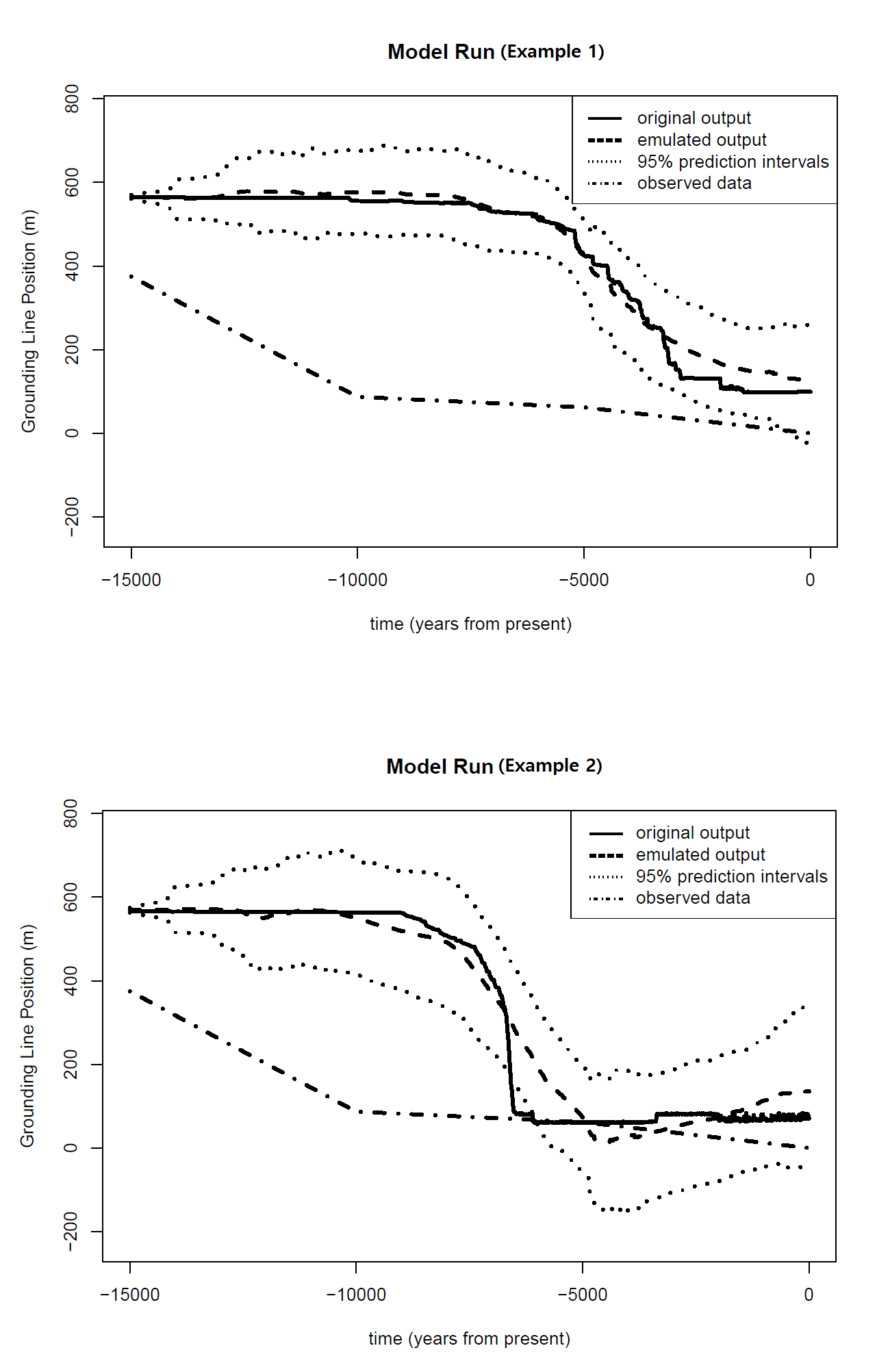
Figure 1: Results for two example parameter settings from the leave-out experiment to verify the performance of the emulator for past grounding line positions. Results for other parameter settings are qualitatively similar to the results shown here. In general, the emulated grounding positions are similar to those from the actual model runs. For comparison we have also added the reconstructed grounding line position observations.

Before calibration, we verified the performance of our emulators through separate leave-out experiments for each emulator $\boldsymbol{\eta}$ and $\boldsymbol{\psi}$. In each experiment we leave out a group of model runs around the center of the parameter space from the ensemble and try to recover them using an emulator constructed based on the remaining model runs. We have left out 82 model runs for the modern binary ice patterns and 60 for the past grounding line positions since we use a smaller number of model runs to emulate the grounding line position output ($q=461$) than the modern binary pattern output ($p=625$). Some examples of the comparison results are shown in Figures 1 (for the past grounding line positions) and 2 (for the modern binary patterns). The results show that our emulators can approximate the true model output reasonably well.

4.1 Simulated Example

In this subsection we describe our calibration results based on simulated observations to study how accurately our method recovers the assumed true parameter setting and its corresponding true projected ice volume change. The assumed-true parameter setting that we choose to use here is OCFAC=0.5, CALV=0.5, CRH=0.5, and TAU=0.4 (rescaled to [0,1]), which correspond to OCFAC=1 (non-dimensional), CALV=1 (non-dimensional), CRH=$10^{-7}$ (m/year Pa²), and approximately TAU=2.6 (k year) in the original scale. This is one of the design points that is closest to the center of the parameter space.

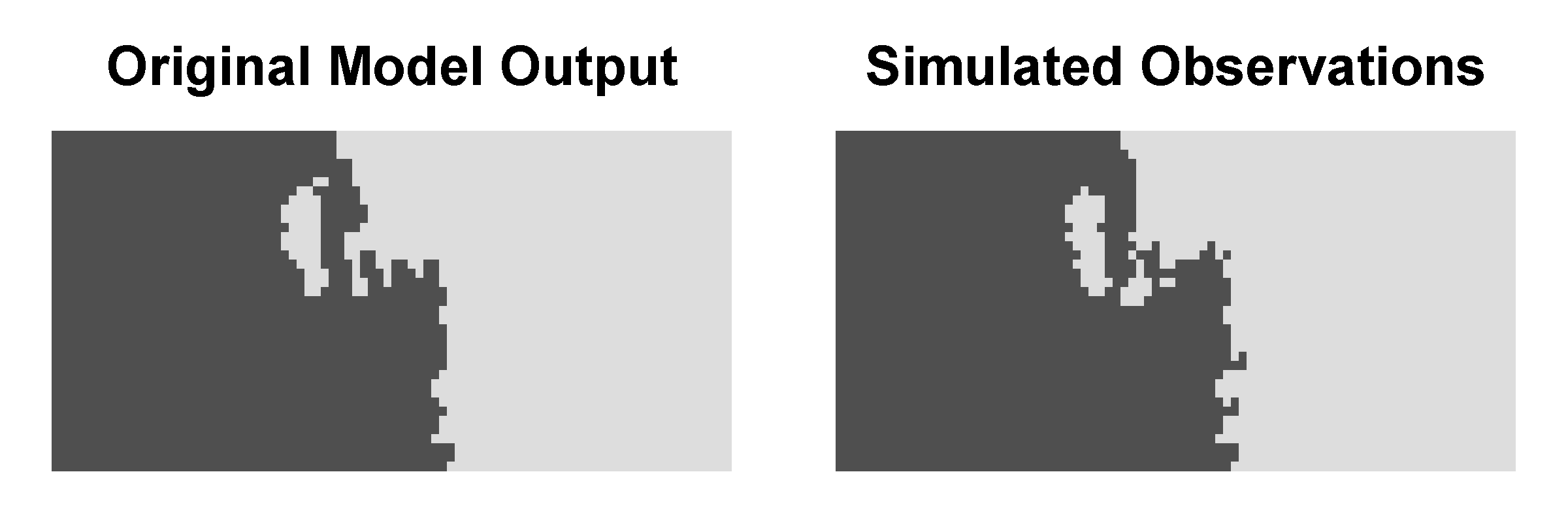
Figure 3: The original model outputs at the assumed true parameter setting and the simulated observations used for the simulated example in Section 4.1. The upper plot is for the past grounding line positions and the lower plots are for the modern binary patterns (light gray for grounded ice and dark gray for no grounded ice).

To represent the presence of model-observation discrepancy we contaminate the model outputs at the true parameter setting with simulated structural errors. We generate simulated errors for the past grounding line positions from a Gaussian process model with zero mean and the covariance defined by the squared exponential function with a sill of 90 m and a range of 10,500 years. The generated errors represent a situation where the model-observation discrepancy varies slowly and has a persistent trend over time. We generate the discrepancy for the modern binary patterns in a manner that makes them realistic. Our approach is therefore as follows. We use the original model output and observational data for the ice thickness pattern used to derived the modern binary patterns. We first choose the “best” 90% model runs (i.e. exclude the “worst” 10% model runs) that are closest to the modern observations in terms of the mean squared differences and take pixel-wise averages for the selected model runs to derive a common thickness pattern. We then subtract the common thickness pattern from the observational data to derive the common discrepancy pattern in terms of the ice thickness. By subtracting this discrepancy pattern from the ice thickness pattern for the assumed truth and dichotomizing the resulting thickness pattern into a binary ice-no ice pattern, we obtain simulated observations for the modern binary pattern. We illustrate the resulting simulated observations in Figure 3.

Depending on the computational environment, the emulation step typically takes several minutes to half an hour. The computation in the calibration step requires about 240 hours to obtain an MCMC sample of size 70,000. The values of MCMC standard errors (Jones et al., 2006; Flegal et al., 2008) suggest that the sample size is large enough to estimate the posterior mean. We have also compared the marginal densities estimated from the first half the MCMC chain and the whole chain and confirmed that the chain is stable.

The probability density plots in Figure 4 show that the posterior has a high probability mass around the assumed truth and hence indicate that our approach can recover the true parameter setting. However, the results also show that parameter settings other than the assumed truth have high probability densities, suggesting that settings other than the assumed truth can yield similar outputs to the simulated observations. Interestingly the joint posterior density for TAU and OCFAC shows that these two parameters have a strong nonlinear interaction with each other.

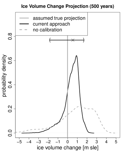
Figure 5: Predictive distribution for the ice volume change projection based on the simulated observations described in Section 4.1. The gray solid line shows the assumed truth. The black solid and the gray dashed lines respectively show the predictive distributions with and without calibration using our approach. The result shows that our approach can recover the assumed truth and significantly reduce the uncertainty in projection.

Figure 5 shows the resulting projection for ice volume change for 500 years from present. To generate the projections we first built an emulator to interpolate the ice volume change values at the existing 625 parameter settings and then converted our MCMC chain for $\boldsymbol{\theta}$ into a Monte Carlo sample for the ice volume change values using the emulator. The result also confirms that our method accurately recovers the assumed-true projection with reasonable uncertainty.

4.2 Calibration Using Real Observations

We are now ready to calibrate the PSU3D-ICE model using the real observational datasets described in Section 2. Our main goal is to investigate whether using information on past grounding line position in our calibration leads to reduced uncertainty and better-constrained projections. To this end, we calibrate the PSU3D-ICE model based on (i) only the modern binary patterns and (ii) both information sources. For (i) we conduct calibration using only the part of the posterior density that is related to $\mathbf{Y}_{2}$ and $\mathbf{Z}_{2}$ and for (ii) we use the entire posterior density. We have obtained MCMC samples with 100,000 for (i) and 47,000 iterations for (ii) and checked its convergence and standard errors, as above.

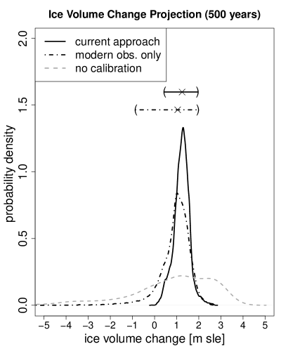
Figure 7: Predictive distribution for the ice volume change projection based on the real observations described in Section 4.2. The black solid line shows the predictive distribution based on our approach using both the past grounding line positions the modern binary patterns and the black dashed and dotted line represents the result based on only the modern binary patterns. The gray dashed line shows the projection without calibration. The results show that using the past grounding line leads to a significantly sharper projection by removing the unrealistic ice volume increase in the results solely based on the modern observations.

The results clearly show the utility of using past grounding line positions in calibrating the PSD3D-ICE model. Figure 6 shows that using the past grounding line positions in our calibration drastically reduces parametric uncertainty. The ice volume change projection based on both information sources also has significantly less uncertainty than that based only on the modern binary patterns (Figure 7). In particular, using the grounding line positions in calibration eliminates the probability mass below 0 m sea level equivalent in the predictive distribution. This improvement is due to the fact that some parameter settings result in very unrealistic ice sheet behavior from the last glacial maximum to the present day, but give modern ice coverage patterns that are close to the current state. See the next subsection for further discussion.

Note that the calibration results in Figure 6 (a) are somewhat different from the results based on the same observational data set shown by Chang et al. (2015), because there are 6 other parameters that are varied in the ensemble used by Chang et al. (2015), which are fixed by expert judgment in this experiment.

4.3 Insights

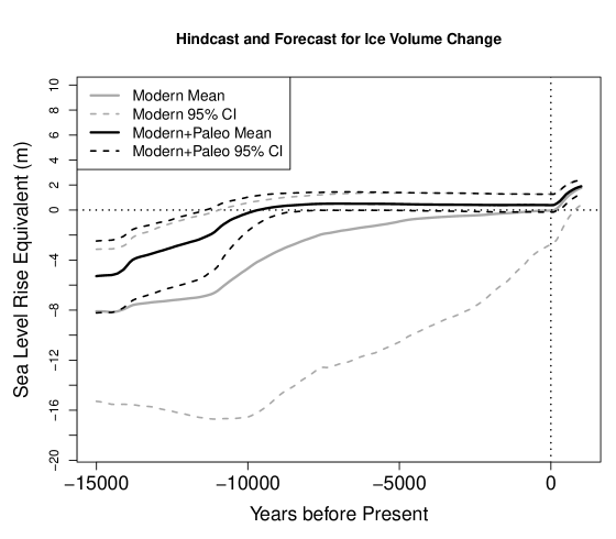
Figure 8: The mean (solid lines) and point-wise 95% predictoin limits (dashed lines) for projected ice volume changes based on the modern binary patterns only (gray) and the past grounding line positions and modern binary patterns (black). Negative values on y-axis indicate the ice volume is larger than the modern value. The prediction limits based only on modern binary patterns contain trajectories that start from excessive amount of ice volume and show very fast ice volume decay. The prediction limits based on both sources of information rule out such unrealistic trajectories.

The results presented in the previous subsection clearly indicate that using the past grounding line position leads to better calibration results with less parametric uncertainties and in turn sharper future ice volume change projections. The hindcast and forecast of ice volume changes based on different data sources in Figure 8 clearly show the reason for this improvement. The 95% prediction intervals show that using the information from past grounding line positions significantly reduces the uncertainties in ice volume change trajectories by ruling out the parameter settings that generate unrealistic past ice sheet behavior. In particular, some parameter settings produce ice sheets that start from a very high ice volume around 15,000 years ago and then show unrealistically rapid ice volume loss, thereby resulting in a modern ice volume that is close to the observed value. These parameter settings are the cause of the left tail of volume change distributions based on the modern binary pattern only. Using paleo data rules out these parameter settings, thereby cutting off the left tail and reducing parametric uncertainty.

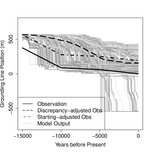
Figure 9: The grounding line position time series from the observational data set (black solid line), observational data adjusted by the discrepancy term (black dashed line), observational data shifted to have the same starting point as the fully adjusted data (dashed and dotted black line), and the model outputs at the input parameter settings $\boldsymbol{\theta}_{1},\dots,\boldsymbol{\theta}_{p}$ (gray lines). The discrepancy term shifts the observational data to match the starting grounding line position to the model outputs, which is similar to using anomalies.

The credibility of this result of course depends on (i) how the model can reliably reproduce the past grounding line time series and (ii) how our calibration method accounts for the model-observation discrepancy. Figure 9 shows the grounding line position time series from the model outputs at the parameter settings $\boldsymbol{\theta}_{1},\dots,\boldsymbol{\theta}_{q}$ and the observational data. It also shows the observational time series corrected by the discrepancy term $\mathbf{K}_{1,d}\boldsymbol{\nu}_{1}$. The discrepancy automatically accounts for the fact that all the model time series start further inland than the observed starting points. Hence, this is analogous to working with anomalies (difference between an observed values and a standard reference value). The use of anomalies is common in paleoclimate modeling. That is, the modeled change in a quantity is considered more reliable than the modeled absolute value, because the model errors that remain constant through time cancel when differences are taken. The model change can either be the difference from the initial model state, or the difference from a “control” simulation of an observed state. The difference is added to the observed quantity to yield a more robust model projection. This is equivalent here to uniformly shifting the observed grounding-line positions to coincide with the mean model initial position at 15,000 years before present (Figure 9).

In addition, we also show another corrected observed time series in which only the starting position is matched with the discrepancy-adjusted observed time series discussed above. The difference between this time series (dashed-dotted line in Figure 9) and the fully corrected time series (dashed line in Figure 9) can be viewed as the estimated discrepancy in anomaly. Although the modeled and observed anomalies clearly show a certain degree of discrepancy, the observed anomaly still allows us to rule out the model runs that showed too small or too large total grounding line position changes over 15,000 years. Therefore the observed grounding line positions still provide useful information for reducing parametric uncertainty.

5 Discussion and Caveats

5.1 Discussion

In this work we have proposed a computationally efficient approach to calibrating WAIS models using two different sources of information, the past grounding line positions and the modern binary spatial patters. Using the proposed approach, we have successfully calibrated the PSU-3D ice model and generated the WAIS volume change projections. Results from a simulated example indicate that our method recovers the true parameters with reasonably small uncertainties as well as provides useful information on interactions between parameters. Results based on the real observations indicate that using the paleo-record significantly reduces parametric uncertainty and leads to better-constrained projections by removing the probability for unrealistic ice volume increase in the predictive distribution.

Several recent modeling studies of Antarctic Ice Sheet variations have used heuristic approaches to study parametric uncertainties, mostly applied to ice-sheet retreat since the last glacial maximum about 15,000 years ago (Whitehouse et al., 2012b, a; Briggs et al., 2013; Briggs and Tarasov, 2013; Briggs et al., 2014; Golledge et al., 2014; Maris et al., 2015). Using highly aggregated data and less statistically formal frameworks, these studies try to reduce the parametric uncertainties based on geologic data around Antarctica. By and large our results are consistent with the parameter values found in these studies, while also reducing uncertainties about the parameters. Other recent modeling studies have projected future Antarctic Ice Sheet response to anthropogenic warming in coming centuries to millennia (Cornford et al., 2015; Feldmann and Levermann, 2015; Golledge et al., 2015; Gomez et al., 2015; Ritz et al., 2015; Winkelmann et al., 2015). These models have been calibrated only over observed small-scale variations of the last few decades. Only a few of these studies use large ensembles, and none use the advanced statistical methods we have developed here, which allow for analyses based on large ensembles and unaggregated data sets. Furthermore, we are able to obtain projections as well as parameter inference in the form of genuine probability distributions, and we take into account potential data-model discrepancies that are ignored by other studies. This allows us to provide uncertainties about our estimates and projections.

5.2 Caveats and Future Directions

One caveat in our calibration model specification is that we do not take into account the dependence between the past grounding line positions and the modern binary patterns. However, we note that the past grounding line positions and the modern binary patterns contain quite different information since two model runs with very different trajectories of past grounding line position often end up with very similar modern binary patterns; this is corroborated by an examination of cross-correlations. Developing a calibration approach based on the generalized principal component analysis that reduces the dimensionality of Gaussian and binary data simultaneously and computes common principal component scores for both data sets is one possible future direction.

Our results are also subject to usual caveats in ice sheet modeling. For example, we use simplified atmospheric conditions for projections, which assumes that atmospheric and oceanic temperatures linearly increase until 150 years after present and stay constant thereafter. Using more detailed warming scenarios is a subject for further work. Another caveat for the present study is the use of coarse-grid global ocean model results to parameterize past basal melting under floating ice shelves. Fine-grid modeling of ocean circulation in Antarctic embayments is challenging, and a topic for further work (e.g. Hellmer et al., 2012) Another improvement will be the use of finer-scale models with higher-order ice dynamics, which as discussed in the introduction, are not quite feasible for the large space and time scales of this study, but should gradually become practical in the near future.

Acknowledgments

We are grateful to A. Landgraf for distributing his code for logistic PCA freely on the Web (https://github.com/andland/SparseLogisticPCA).

This work was partially supported by National Science Foundation through (1) NSF-DMS-1418090 and (2) NSF/OCE/FESD 1202632 and NSF/OPP/ ANT 1341394, (3) Network for Sustainable Climate Risk Management under NSF cooperative agreement GEO1240507, and (4) NSF Statistical Methods in the Atmospheric Sciences Network (Award Nos. 1106862, 1106974, and 1107046). WC was partially supported by (3) and (4), and MH and PA were partially supported by (1) and (3), and DP is partially supported by (1), (2) and (3). All views, errors, and opinions are solely those of the authors.

Appendix A. Computation in Reduced-Dimensional Space

For faster computation we infer $\boldsymbol{\theta}$ and other parameters in the model based on the following dimension-reduced version of the observational data for the past grounding line positions:

$$\mathbf{Z}_{1}^{R}=(\mathbf{K}_{1}^{T}\mathbf{K}_{1})^{-1}\mathbf{K}_{1}^{T}\mathbf{Z}_{1}=\left(\begin{array}[]{c}\boldsymbol{\eta}(\boldsymbol{\theta},\mathbf{Y}_{1}^{R})\\ \boldsymbol{\nu}_{1}\end{array}\right)+(\mathbf{K}_{1}^{T}\mathbf{K}_{1})^{-1}\mathbf{K}_{1}^{T}\boldsymbol{\epsilon}_{1},$$

where $\mathbf{K}_{1}=(\mathbf{K}_{1,y}~{}\mathbf{K}_{1,d})$, which leads to the probability model

$$\mathbf{Z}_{1}^{R}|\boldsymbol{\nu}_{2}\sim N\left(\left(\begin{array}[]{c}\boldsymbol{\mu}_{\boldsymbol{\eta}}\\ \boldsymbol{\mu}_{\boldsymbol{\nu}_{1}|\boldsymbol{\nu}_{2}}\end{array}\right),\left(\begin{array}[]{cc}\boldsymbol{\Sigma}_{\boldsymbol{\eta}}&\mathbf{0}\\ \mathbf{0}&\boldsymbol{\Sigma}_{\boldsymbol{\nu}_{1}|\boldsymbol{\nu}_{2}}\end{array}\right)+\sigma_{\epsilon}^{2}(\mathbf{K}_{1}^{T}\mathbf{K}_{1})^{-1}\right).$$ (8)

The $J_{1}$-dimensional vector $\mu_{\boldsymbol{\eta}}$ and $J_{1}\times J_{1}$ matrix $\Sigma_{\boldsymbol{\eta}}$ are the mean and variance of $\boldsymbol{\eta}(\boldsymbol{\theta},\mathbf{Y}_{1}^{R})$. The $M$-dimensional vector $\boldsymbol{\mu}_{\boldsymbol{\nu}_{1}|\boldsymbol{\nu}_{2}}$ and $M\times M$ matrix $\boldsymbol{\Sigma}_{\boldsymbol{\nu}_{1}|\boldsymbol{\nu}_{2}}$ are the conditional mean and variance of $\boldsymbol{\nu}_{1}$ given $\boldsymbol{\nu}_{2}$ which can be computed as

$$\boldsymbol{\mu}_{\boldsymbol{\nu}_{1}|\boldsymbol{\nu}_{2}} =\frac{1}{\alpha_{2}^{2}}\mathbf{R}_{\nu}\boldsymbol{\nu}_{2},$$

$$\boldsymbol{\Sigma}_{\boldsymbol{\nu}_{1}|\boldsymbol{\nu}_{2}} =\alpha_{1}^{2}\left(\mathbf{I}_{M}-\mathbf{R}_{\nu}\mathbf{R}_{\nu}^{T}\right).$$

Using the likelihood function corresponding to this probability model and some standard prior specification for $\boldsymbol{\theta}$, $\alpha_{1}^{2}$ and $\sigma_{\epsilon}^{2}$ (see Section 4 for details), we can infer the parameters via Markov chain Monte Carlo (MCMC). The computational cost for likelihood evaluation reduces from $\frac{1}{3}n^{3}$ to $\frac{1}{3}(J_{1}+M)^{3}$.

Appendix B. Detailed Description for the Posterior Density based on the Model Specification in Section 3.2.3

The parameters that we estimate in the equations in (5) and (6) are the input parameter $\boldsymbol{\theta}$ (which is our main target), the variance of the i.i.d observational errors for the grounding line positions $\sigma_{\epsilon}^{2}$, coefficients for the emulator term $\boldsymbol{\psi}=\boldsymbol{\psi}(\boldsymbol{\theta},\mathbf{Y}_{2}^{R})$, the coefficients for the discrepancy term for the modern binary pattern $\boldsymbol{\nu}_{2}$, and the variances of $\boldsymbol{\nu}_{1}$ and $\boldsymbol{\nu}_{2}$, $\alpha_{1}^{2}$ and $\alpha_{2}^{2}$. In addition to these parameters we also re-estimate the sill parameters for the emulator $\boldsymbol{\eta}$, $\boldsymbol{\kappa}_{1}=[\kappa_{1,1},\dots,\kappa_{1,J_{1}}]$ (cf. Bayarri et al., 2007; Bhat et al., 2012; Chang et al., 2014b) to account for a possible scale mismatch between the computer model output $\mathbf{Y}_{1}$ and the observational data $\mathbf{Z}_{1}$. However, we do not re-estimate the sill parameters for $\boldsymbol{\psi}$, $\kappa_{2,1},\dots,\kappa_{2,J_{2}}$, since both $\mathbf{Y}_{2}$ and $\mathbf{Z}_{2}$ are binary responses and hence a scaling issue is not likely to occur here; in fact we have found that re-estimating these parameters causes identifiability issues between the emulator term $\mathbf{K}_{2,y}\boldsymbol{\psi}(\boldsymbol{\theta},\mathbf{Y}_{2}^{R})$ and the discrepancy term $\mathbf{K}_{2,d}\boldsymbol{\nu}_{2}$.

The posterior density can be written as

$$\small\pi(\boldsymbol{\theta},\boldsymbol{\psi},\boldsymbol{\kappa}_{1},\boldsymbol{\nu}_{2},\alpha_{1}^{2},\alpha_{2}^{2},\sigma_{\epsilon}^{2},\mathbf{R}_{\nu}|\mathbf{Y}_{1}^{R},\mathbf{Z}_{1}^{R},\mathbf{Y}_{2}^{R},\mathbf{Z}_{2})\propto ~{}L\left(\mathbf{Z}_{1}^{R}|\mathbf{Y}_{1}^{R},\boldsymbol{\theta},\boldsymbol{\kappa}_{1},\alpha_{1}^{2},\sigma_{\epsilon}^{2},\boldsymbol{\nu}_{2},\mathbf{R}_{\nu}\right)$$

$$\times f(\boldsymbol{\kappa}_{1})f(\alpha_{1}^{2})f(\sigma_{\epsilon}^{2})f(\mathbf{R}_{\nu})$$

$$\times L\left(\mathbf{Z}_{2}|\boldsymbol{\psi},\boldsymbol{\nu}_{2}\right)$$

$$\times f\left(\boldsymbol{\psi}|\boldsymbol{\theta},\mathbf{Y}_{2}^{R}\right)f(\boldsymbol{\nu}_{2}|\alpha_{2}^{2})f(\alpha_{2}^{2}),$$

$$\times f(\boldsymbol{\theta})$$

The likelihood function $L\left(\mathbf{Z}_{1}^{R}|\mathbf{Y}_{1}^{R},\boldsymbol{\theta},\boldsymbol{\kappa}_{1},\alpha_{1}^{2},\sigma_{\epsilon}^{2},\boldsymbol{\nu}_{2},\mathbf{R}_{\nu}\right)$ is given by the probability model in (8). For $f(\boldsymbol{\kappa}_{1})=f(\kappa_{1,1},\dots,\kappa_{1,J_{1}})$ we use independent inverse gamma priors with a shape parameter of 50 and scale parameters specified in a way that the modes of the densities coincide with the estimated values of $\kappa_{1,1},\dots,\kappa_{1,J_{1}}$ from the emulation stage. We assign a vague prior $IG(2,3)$ for $f\left(\alpha_{1}^{2}\right)$, $f\left(\alpha_{2}^{2}\right)$, and $f\left(\sigma_{\epsilon}^{2}\right)$, and a uniform prior for $f(\boldsymbol{\theta})$ whose support is defined by the range of design points $\boldsymbol{\theta}_{1},\dots,\boldsymbol{\theta}_{p}$. The likelihood function $L(\mathbf{Z}_{2}|\boldsymbol{\psi},\boldsymbol{\nu}_{2})$ is defined as

$$L\left(\mathbf{Z}_{2}|\boldsymbol{\psi},\boldsymbol{\nu}_{2}\right) \propto\prod_{j=1}^{n}\left(\frac{\exp(\lambda_{j})}{1+\exp(\lambda_{j})}\right)^{Z_{2}(\mathbf{s}_{j})}\left(\frac{1}{1+\exp(\lambda_{j})}\right)^{1-Z_{2}(\mathbf{s}_{j})},$$

where $\lambda_{j}$ is the $j$th element of $\boldsymbol{\lambda}$ in (6). The conditional density $f\left(\boldsymbol{\psi}|\boldsymbol{\theta},\mathbf{Y}_{2}^{R}\right)$ is given by the Gaussian process emulator $\boldsymbol{\psi}(\boldsymbol{\theta},\mathbf{Y}_{2}^{R})$. The conditional density $f\left(\boldsymbol{\nu}_{2}|\alpha_{2}^{2}\right)$ is defined by the model $\boldsymbol{\nu}_{2}\sim N(0,\alpha_{2}^{2}\mathbf{I}_{L})$. The prior density $f(\mathbf{R}_{\nu})$ is defined as

$$\prod_{i=1}^{M}\prod_{j=1}^{L}I(-1<\rho_{\nu,i,j}<1)\cdot I(\mathbf{I}_{M}-\mathbf{R}_{\nu}\mathbf{R}_{\nu}^{T}\mbox{ is positive definite}),$$

where $I(\cdot)$ is the indicator function and $\rho_{\nu,i,j}$ is the $(i,j)$th element of $\mathbf{R}_{\nu}$.

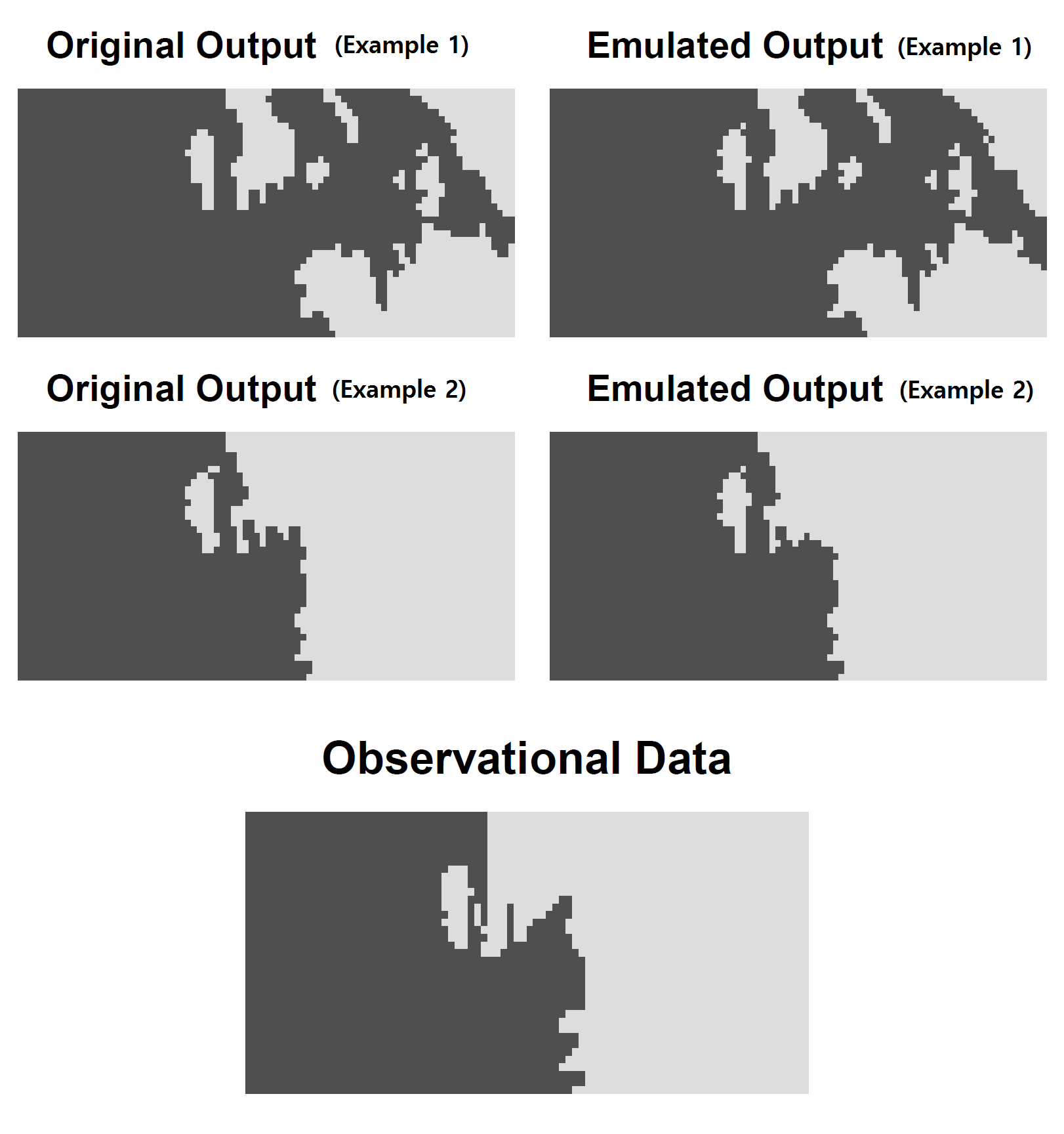
Figure 2: Results for two example parameter settings from the leave-out experiment to verify the performance of the emulator for modern binary patterns (light gray for grounded ice and dark gray for no grounded ice). Results for other parameter settings are similar to the ones presented here. In general, the emulator can accurately approximate the binary patterns from the actual model runs. For comparison we have also included the observed modern binary patten.

Figure 4: Posterior density for input parameters from the perfect model experiment described in Section 4.1. The black dashed lines represent the assumed parameter settings. The result indicates that our method can recover the true input parameter setting by assigning high posterior density around the truth. The joint density in the upper left panel shows that OCFAC and TAU have a strong non-linear interaction.

(a) Modern Binary Patterns Only

(b) Modern Binary Patterns and Past Grounding Line Positions

Figure 6: Posterior density for input parameters based on the actual observational data sets (see Section for details Section 4.2). Using both information sources leads to significantly less uncertainty in estimating input parameters.

References

- Applegate et al. (2012) P.J. Applegate, N. Kirchner, E.J. Stone, K. Keller, and R. Greve. An assessment of key model parametric uncertainties in projections of Greenland Ice Sheet behavior. The Cryosphere, 6(3):589–606, 2012.
- Bayarri et al. (2007) M.J. Bayarri, J.O. Berger, J. Cafeo, G. Garcia-Donato, F. Liu, J. Palomo, R.J. Parthasarathy, R. Paulo, J. Sacks, and D. Walsh. Computer model validation with functional output. The Annals of Statistics, 35(5):1874–1906, 2007.
- Bhat et al. (2010) K.S. Bhat, M. Haran, and M. Goes. Computer model calibration with multivariate spatial output: A case study. In M.H. Chen, P. Müller, D. Sun, K. Ye, and D.K. Dey, editors, Frontiers of Statistical Decision Making and Bayesian Analysis, pages 168–184. Springer, 2010.
- Bhat et al. (2012) K.S. Bhat, M. Haran, R. Olson, and K. Keller. Inferring likelihoods and climate system characteristics from climate models and multiple tracers. Environmetrics, 23(4):345–362, 2012.
- Bindschadler et al. (2013) Robert A Bindschadler, Sophie Nowicki, Ayako Abe-Ouchi, Andy Aschwanden, Hyeungu Choi, Jim Fastook, Glen Granzow, Ralf Greve, Gail Gutowski, Ute Herzfeld, Charles Jackson, Jesse Johnson, Constantine Khroulev, Anders Levermann, William H. Lipscomb, Maria A. Martin, Mathieu Morlighem, Byron R. Parizek, David Pollard, Stephen F. Price, Diandong Ren, Fuyuki Saito, Tatsuru Sato, Hakime Seddik, Helene Seroussi, Kunio Takahashi, Ryan Walker, and Wei Li Wang. Ice-sheet model sensitivities to environmental forcing and their use in projecting future sea level (the searise project). Journal of Glaciology, 59(214):195–224, 2013.
- Briggs et al. (2013) R Briggs, D Pollard, and L Tarasov. A glacial systems model configured for large ensemble analysis of Antarctic deglaciation. The Cryosphere, 7(2):1533–1589, 2013.
- Briggs and Tarasov (2013) Robert D Briggs and Lev Tarasov. How to evaluate model-derived deglaciation chronologies: a case study using Antarctica. Quarterly Science Review, 63:109–127, 2013.
- Briggs et al. (2014) Robert D Briggs, David Pollard, and Lev Tarasov. A data-constrained large ensemble analysis of Antarctic evolution since the Eemian. Quarterly Science Review, 103:91–115, 2014.
- Brynjarsdóttir and O’Hagan (2014) Jennỳ Brynjarsdóttir and Anthony O’Hagan. Learning about physical parameters: The importance of model discrepancy. Inverse Problems, 30(11):114007, 2014.
- Chang et al. (2014a) W. Chang, P. Applegate, H. Haran, and K. Keller. Probabilistic calibration of a greenland ice sheet model using spatially-resolved synthetic observations: toward projections of ice mass loss with uncertainties. Geoscientific Model Development, 7:1933–1943, 2014a.
- Chang et al. (2014b) Won Chang, Murali Haran, Roman Olson, and Klaus Keller. Fast dimension-reduced climate model calibration and the effect of data aggregation. The Annals of Applied Statistics, 8(2):649–673, 2014b.
- Chang et al. (2015) Won Chang, Murali Haran, Patrick Applegate, and David Pollard. Calibrating an ice sheet model using high-dimensional binary spatial data. Journal of the American Statistical Association, 2015. in press.
- Cornford et al. (2015) Stephen Leslie Cornford, DF Martin, AJ Payne, EG Ng, AM Le Brocq, RM Gladstone, TL Edwards, SR Shannon, Cécile Agosta, MR Van Den Broeke, H.H. Hellmer, G. Krinner, S.R.M. Ligtenberg, R. Timmermann, and D.G. Vaughan. Century-scale simulations of the response of the West Antarctic Ice Sheet to a warming climate. 9:1579–1600, 2015.
- Favier et al. (2014) L Favier, G Durand, SL Cornford, GH Gudmundsson, O Gagliardini, F Gillet-Chaulet, T Zwinger, AJ Payne, and AM Le Brocq. Retreat of pine island glacier controlled by marine ice-sheet instability. Nature Climate Change, 4:171–121, 2014.
- Feldmann and Levermann (2015) Johannes Feldmann and Anders Levermann. Collapse of the west antarctic ice sheet after local destabilization of the amundsen basin. Proceedings of the National Academy of Sciences of the United States of America, 112(46):14191–14196, 2015.
- Flegal et al. (2008) J. M. Flegal, M. Haran, and G. L. Jones. Markov chain monte carlo: Can we trust the third significant figure? Statistical Science, 23(2):250–260, 2008.
- Fretwell et al. (2013) P Fretwell, Hamish D Pritchard, David G Vaughan, J. L. Bamber, N. E. Barrand, R Bell, C Bianchi, R. G. Bingham, D. D. Blankenship, G Casassa, G. Catania, D. Callens, H. Conway, A.J. Cook, H.F.J. Corr, D. Damaske, V. Damm, F. Ferraccioli, R. Forsberg, S. Fujita, Y. Gim, P. Gogineni, J.A. Griggs, R.C.A. Hindmarsh, P. Holmlund, J.W. Holt, R.W. Jacobel, A. Jenkins, W. Jokat, T. Jordan, E.C. King, J. Kohler, W. Krabill, M. Riger-Kusk, K.A. Langley, G. Leitchenkov, C. Leuschen, B.P. Luyendyk, K. Matsuoka, J. Mouginot, F.O. Nitsche, Y. Nogi, O.A. Nost, S.V. Popov, E. Rignot, D.M. Rippin, A. Rivera, J. Roberts, N. Ross, M.J. Siegert, A.M. Smith, D. Steinhage, M. Studinger, B. Sun, B.K. Tinto, B.C. Welch, D. Wilson, D.A. Young, C. Xiangbin, and A. Zirizzotti. Bedmap2: improved ice bed, surface and thickness datasets for antarctica. The Cryosphere, 7(1):375–393, 2013.
- Gladstone et al. (2012) Rupert M Gladstone, Victoria Lee, Jonathan Rougier, Antony J Payne, Hartmut Hellmer, Anne Le Brocq, Andrew Shepherd, Tamsin L Edwards, Jonathan Gregory, and Stephen L Cornford. Calibrated prediction of pine island glacier retreat during the 21st and 22nd centuries with a coupled flowline model. Earth and Planetary Science Letters, 333:191–199, 2012.
- Golledge et al. (2014) NR Golledge, L Menviel, L Carter, CJ Fogwill, MH England, G Cortese, and RH Levy. Antarctic contribution to meltwater pulse 1A from reduced Southern Ocean overturning. Nature communications, 5, 2014.
- Golledge et al. (2015) NR Golledge, DE Kowalewski, TR Naish, RH Levy, CJ Fogwill, and EGW Gasson. The multi-millennial Antarctic commitment to future sea-level rise. Nature, 526(7573):421–425, 2015.
- Gomez et al. (2015) Natalya Gomez, David Pollard, and David Holland. Sea-level feedback lowers projections of future Antarctic Ice-Sheet mass loss. Nature communications, 6, 2015.
- Hastie et al. (2009) T. Hastie, R. Tibshirani, and J. Friedman. The Elements of Statistical Learning: Data Mining, Inference, and Prediction. Springer, New York, 2009.
- Hellmer et al. (2012) Hartmut H Hellmer, Frank Kauker, Ralph Timmermann, Jürgen Determann, and Jamie Rae. Twenty-first-century warming of a large antarctic ice-shelf cavity by a redirected coastal current. Nature, 485(7397):225–228, 2012.
- Higdon et al. (2008) D. Higdon, J. Gattiker, B. Williams, and M. Rightley. Computer model calibration using high-dimensional output. Journal of the American Statistical Association, 103(482):570–583, 2008.
- Jones et al. (2006) G. Jones, M. Haran, B. S. Caffo, and R. Neath. Fixed-width output analysis for markov chain monte carlo. Journal of the American Statistical Association, 101(476):1537–1547, 2006.
- Joughin et al. (2014) Ian Joughin, Benjamin E Smith, and Brooke Medley. Marine ice sheet collapse potentially under way for the thwaites glacier basin, west antarctica. Science, 344(6185):735–738, 2014.
- Kennedy and O’Hagan (2001) M.C. Kennedy and A. O’Hagan. Bayesian calibration of computer models. Journal of the Royal Statistical Society. Series B (Statistical Methodology), 63(3):425–464, 2001.
- Kirshner et al. (2012) Alexandra E Kirshner, John B Anderson, Martin Jakobsson, Matthew O’Regan, Wojciech Majewski, and Frank O Nitsche. Post-lgm deglaciation in pine island bay, west antarctica. Quarterly Science Review, 38:11–26, 2012.
- Larter et al. (2014) Robert D Larter, John B Anderson, Alastair GC Graham, Karsten Gohl, Claus-Dieter Hillenbrand, Martin Jakobsson, Joanne S Johnson, Gerhard Kuhn, Frank O Nitsche, and James A Smith. Reconstruction of changes in the amundsen sea and bellingshausen sea sector of the west antarctic ice sheet since the last glacial maximum. Quarterly Science Review, 100:55–86, 2014.
- Lempert et al. (2012) Robert Lempert, Ryan L Sriver, and Klaus Keller. Characterizing Uncertain Sea Level Rise Projections to Support Investment Decisions. California Energy Commission, Publication Number: CEC-500-2012-056, 2012.
- Liu et al. (2009) Z Liu, BL Otto-Bliesner, F He, EC Brady, R Tomas, PU Clark, AE Carlson, J Lynch-Stieglitz, W Curry, E Brook, D. Erickson, R. Jacob, J. Kutzbach, and J. Cheng. Transient simulation of last deglaciation with a new mechanism for bølling-allerød warming. Science, 325(5938):310–314, 2009.
- Maris et al. (2015) MNA Maris, JM Van Wessem, WJ Van De Berg, B De Boer, and J Oerlemans. A model study of the effect of climate and sea-level change on the evolution of the antarctic ice sheet from the last glacial maximum to 2100. Climate Dynamics, 45(3-4):837–851, 2015.
- McNeall et al. (2013) DJ McNeall, PG Challenor, JR Gattiker, and EJ Stone. The potential of an observational data set for calibration of a computationally expensive computer model. Geoscientific Model Development, 6(5):1715–1728, 2013.
- Pollard and DeConto (2012a) D Pollard and R. M. DeConto. Description of a hybrid ice sheet-shelf model, and application to Antarctica. Geoscientific Model Development, 5:1273–1295, 2012a.
- Pollard and DeConto (2012b) D Pollard and R. M. DeConto. A simple inverse method for the distribution of basal sliding coefficients under ice sheets, applied to Antarctica. The Cryosphere, 6(2):1405–1444, 2012b.
- Pollard and DeConto (2009) David Pollard and Robert M DeConto. Modelling West Antarctic ice sheet growth and collapse through the past five million years. Nature, 458(7236):329–332, 2009.
- Pritchard et al. (2012) H. D. Pritchard, S. R. M. Ligtenberg, H. A. Fricker, D. G. Vaughan, M. R. Van den Broeke, and L Padman. Antarctic ice-sheet loss driven by basal melting of ice shelves. Nature, 484(7395):502–505, 2012.
- RAISED Consortium (2014) RAISED Consortium. A community-based geological reconstruction of antarctic ice sheet deglaciation since the last glacial maximum. Quarterly Science Review, 100:1–9, 2014.
- Ritz et al. (2015) Catherine Ritz, Tamsin L Edwards, Gaël Durand, Antony J Payne, Vincent Peyaud, and Richard CA Hindmarsh. Potential sea-level rise from Antarctic ice-sheet instability constrained by observations. Nature, 528(7580):115–118, 2015.
- Sacks et al. (1989) J. Sacks, W.J. Welch, T.J. Mitchell, and H.P. Wynn. Design and analysis of computer experiments. Statistical Science, 4(4):409–423, 1989.
- Stone et al. (2010) E.J. Stone, D.J. Lunt, I.C. Rutt, and E. Hanna. Investigating the sensitivity of numerical model simulations of the modern state of the greenland ice-sheet and its future response to climate change. The Cryosphere, 4(3):397–417, 2010.
- Whitehouse et al. (2012a) P. L. Whitehouse, M. J. Bentley, G. A. Milne, M. A. King, and I. D. Thomas. A new glacial isostatic model for Antarctica: calibrated and tested using observations of relative sea-level change and present-day uplifts. Geophysical Journal International, 190:1464–1482, 2012a.
- Whitehouse et al. (2012b) P.L. Whitehouse, M.J. Bentley, and A.M. Le Brocq. A deglacial model for Antarctica: geological constraints and glaciological modeling as a basis for a new model of Antarctic glacial isostatic adjustment. Quarterly Science Review, 32:1–24, 2012b.
- Winkelmann et al. (2015) Ricarda Winkelmann, Anders Levermann, Andy Ridgwell, and Ken Caldeira. Combustion of available fossil fuel resources sufficient to eliminate the Antarctic Ice Sheet. Sceince Advances, 1(8):e1500589, 2015. doi: 10.1126/sciadv.1500589.