Solution of a generalised Boltzmann’s equation for non-equilibrium charged particle transport via localised and delocalised states

Abstract

We present a general phase-space kinetic model for charged particle transport through combined localised and delocalised states, capable of describing scattering collisions, trapping, detrapping and losses. The model is described by a generalised Boltzmann equation, for which an analytical solution is found in Fourier-Laplace space. The velocity of the centre of mass (CM) and the diffusivity about it are determined analytically, together with the flux transport coefficients. Transient negative values of the free particle CM transport coefficients can be observed due to the trapping to, and detrapping from, localised states. A Chapman-Enskog type perturbative solution technique is applied, confirming the analytical results and highlighting the emergence of a density gradient representation in the weak-gradient hydrodynamic regime. A generalised diffusion equation with a unique global time operator is shown to arise, reducing to the standard diffusion equation and a Caputo fractional diffusion equation in the normal and dispersive limits. A subordination transformation is used to solve the generalised diffusion equation by mapping from the solution of a corresponding standard diffusion equation.

I Introduction

Normal transport, as described by the diffusion equation, has a mean squared displacement that scales linearly with time, $t$. Dispersive transport, however, is often defined by a mean squared displacement that scales sublinearly, proportional to $t^{\alpha}$ where $0<\alpha<1$ (Metzler and Klafter, 2000). Physically, this arises due to the presence of traps causing particles to become immobilised (localised states) for extended periods of time and resulting in fundamentally slower transport (Scher and Montroll, 1975). A number of physical systems have the potential to exhibit dispersive transport. For example, in organic semiconductors, and other disordered media, trapped states arise due to local imperfections or variation in the energetic landscape (Scher and Montroll, 1975; Sibatov and Uchaikin, 2007). Electron transport in certain liquids can be influenced through electrons becoming trapped in (localised) bubble states (see e.g. (Mauracher et al., 2014; Borghesani and Santini, 2002)), giving rise to dispersive electronic transport in liquid neon (Sakai et al., 1992). Similar trapping processes occur for positronium in bubbles (see e.g. (Stepanov et al., 2012, 2002; Drachman et al., 2000)) and positrons annihilation on induced clusters (see e.g. (Colucci et al., 2011)).

A consequence of dispersive systems, especially those with long-lived traps, is their dependence on their history. The diffusion equation, which uses a local time operator, is fundamentally incapable of describing such memory effects. Mathematically, an adequate model for dispersive transport requires a global time operator that acts on the entire history of the system. One successful approach for modelling dispersive transport is by replacing the the local time derivative in the diffusion equation with a global fractional time derivative of order $\alpha$ (Barkai, 2001; Metzler et al., 1999). This resulting fractional diffusion equation describes memory effects while also satisfying the required sublinear scaling of the mean squared displacement.

However, fractional diffusion equations still share the same spatial operator as the standard diffusion equation which implies implicitly an assumption of small spatial gradients. At the same time, the memory of the initial condition can cause large spatial gradients to persist for all time. This inconsistency challenges the validity of fractional diffusion equations. This has been addressed by using phase-space kinetic models for dispersive transport that make no such assumptions on the size of spatial gradients (Robson and Blumen, 2005; Philippa et al., 2014). Specifically, these have made use of a Boltzmann equation with a generalisation of the Bhatnagar-Gross-Krook (BGK) collision operator (Bhatnagar et al., 1954), the standard collision operator in semiconductor physics. In our previous work (Philippa et al., 2014), trapping and detrapping is considered equivalent to a BGK collision scattering event occurring after a delay governed by a trapping time distribution. That study did not consider scattering as a separate process from trapping, thereby limiting the model to situations where trapping dominates over scattering. However, scattering events are key to transport in delocalised states, such as in the conduction band of a semiconductor. The present study builds upon previous work by incorporating a genuine scattering model into a kinetic equation with memory of past trapping events. The new, proposed model also incorporates loss mechanisms such as charged carrier recombination.

In Section II of this paper, we present a generalised Boltzmann equation with a BGK collision operator to describe transport via delocalised states, a delayed BGK operator to model trapping and detrapping associated with localised (trapped) states, and loss terms corresponding to free and trapped particle recombination. In Section III, we determine an analytical Fourier-Laplace space solution of this model. This analytical solution is used, among other things, to determine analytical expressions for phase-space averaged moments of the generalised Boltzmann equation. Spatial moments provide transport coefficients describing the the motion of the centre of mass, while velocity moments are used in conjunction to describe the particle flux using flux transport coefficients. In Section IV, the model is explored in the weak-gradient hydrodynamic regime where it is shown to coincide with both a standard diffusion equation and a generalised diffusion equation with history dependence. In Section V, the model is also shown to coincide with a Caputo fractional diffusion equation in the particular case where transport is dispersive. In Section VI, the solution of the generalised diffusion equation is expressed as a subordination transformation of the solution of a corresponding standard diffusion equation. Finally, in Section VII, we present conclusions and possible avenues for future work.

II Generalised Boltzmann equation

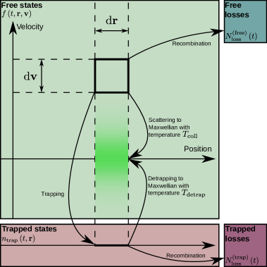
Figure 1: Phase-space diagram illustrating the collision, trapping, detrapping and recombination processes considered in the model defined by Eqs. (1)-(8).

We will consider a generalised phase-space kinetic model describing the transport of free particles undergoing collisions, trapping, detrapping and recombination as illustrated in Figure 1. The free particles will be described by the phase-space distribution function $f\left(t,\mathbf{r},\mathbf{v}\right)$ which satisfies the Boltzmann equation

$$\left(\frac{\partial}{\partial t}+\mathbf{v}\cdot\frac{\partial}{\partial\mathbf{r}}+\mathbf{a}\cdot\frac{\partial}{\partial\mathbf{v}}\right)f\left(t,\mathbf{r},\mathbf{v}\right)=-\nu_{\mathrm{coll}}\left[f\left(t,\mathbf{r},\mathbf{v}\right)-n\left(t,\mathbf{r}\right)w\left(\alpha_{\mathrm{coll}},v\right)\right]\\ -\nu_{\mathrm{trap}}\left[f\left(t,\mathbf{r},\mathbf{v}\right)-\Phi\left(t\right)\ast n\left(t,\mathbf{r}\right)w\left(\alpha_{\mathrm{detrap}},v\right)\right]-\nu_{\mathrm{loss}}^{\left(\mathrm{free}\right)}f\left(t,\mathbf{r},\mathbf{v}\right),$$ (1)

where collision, trapping and free particle loss rates are respectively denoted $\nu_{\mathrm{coll}}$, $\nu_{\mathrm{trap}}$ and $\nu_{\mathrm{loss}}^{\left(\mathrm{free}\right)}$ and the free particle number density is defined $n\left(t,\mathbf{r}\right)\equiv\int\mathrm{d}\mathbf{v}f\left(t,\mathbf{r},\mathbf{v}\right)$. Collisions are described above by the Bhatnagar-Gross-Krook (BGK) collision operator (Bhatnagar et al., 1954). Specifically, free particles are instantaneously scattered to a Maxwellian distribution of velocities of temperature $T_{\mathrm{coll}}$. The Maxwellian velocity distribution is defined

$$w\left(\alpha,v\right) \equiv \left(\frac{\alpha^{2}}{2\pi}\right)^{\frac{3}{2}}\exp\left(-\frac{\alpha^{2}v^{2}}{2}\right),$$ (2)

$$\alpha^{2} \equiv \frac{m}{k_{\mathrm{B}}T},$$ (3)

where $m$ is the free particle mass, $k_{\mathrm{B}}$ is the Boltzmann constant and $T$ is the temperature of the scattered particles. Similarly, trapping and detrapping processes occur as described by a delayed BGK model (Philippa et al., 2014), according to an effective waiting time distribution $\Phi(t)$, with trapped particles eventually detrapped with a Maxwellian velocity distribution of temperature $T_{\mathrm{detrap}}$. To define this waiting time distribution, consider the simple case of traps of fixed duration $\tau$. Particles enter traps at the rate $\nu_{\mathrm{trap}}n\left(t,\mathbf{r}\right)$ and so leave traps at this same rate $\tau$ units of time in the future. From the present perspective this rate of detrapping is $\nu_{\mathrm{trap}}n\left(t-\tau,\mathbf{r}\right)$. More generally, for a distribution of trapping times $\phi\left(t\right)$, the rate of detrapping is now written as the convolution

$$\nu_{\mathrm{trap}}\phi\left(t\right)\ast n\left(t,\mathbf{r}\right)=\nu_{\mathrm{trap}}\int_{0}^{t}\mathrm{d}\tau\phi\left(\tau\right)n\left(t-\tau,\mathbf{r}\right).$$ (4)

Here, the quantity $\mathrm{d}P\equiv\phi\left(\tau\right)\mathrm{d}\tau$ can be interpreted as an infinitesimal probability that particles will remain trapped for duration $\tau$. Note that this expression does not take into account the possibility that particles may undergo trap-based losses instead of detrapping. As trapped particles are being lost exponentially at the rate $\nu_{\mathrm{loss}}^{\left(\mathrm{trap}\right)}$, the probability of detrapping decays correspondingly, $\mathrm{d}P=\mathrm{e}^{-\nu_{\mathrm{loss}}^{\left(\mathrm{trap}\right)}\tau}\phi\left(\tau\right)\mathrm{d}\tau$. That is, we have now the effective waiting time distribution

$$\Phi\left(t\right)\equiv\mathrm{e}^{-\nu_{\mathrm{loss}}^{\left(\mathrm{trap}\right)}t}\phi\left(t\right).$$ (5)

As the trapped particles are localised in configuration space, we describe them with the number density $n_{\mathrm{trap}}\left(t,\mathbf{r}\right)$ that satisfies the continuity equation

$$\frac{\partial}{\partial t}n_{\mathrm{trap}}\left(t,\mathbf{r}\right)=\nu_{\mathrm{trap}}\left(1-\Phi\ast\right)n\left(t,\mathbf{r}\right)-\nu_{\mathrm{loss}}^{\left(\mathrm{trap}\right)}n_{\mathrm{trap}}\left(t,\mathbf{r}\right),$$ (6)

where $\nu_{\mathrm{loss}}^{\left(\mathrm{trap}\right)}$ is the loss rate of trapped particles. Although the loss processes of the free and trapped particles can occur through various mechanisms (e.g. recombination, attachment, …), for simplicity we will refer to all losses as being due to recombination processes. The number of free and trapped particles that undergo recombination, $N_{\mathrm{\mathrm{loss}}}^{\left(\mathrm{free}\right)}\left(t\right)$ and $N_{\mathrm{\mathrm{loss}}}^{\left(\mathrm{trap}\right)}\left(t\right)$, can be counted accordingly

$$\frac{\mathrm{d}}{\mathrm{d}t}N_{\mathrm{\mathrm{loss}}}^{\left(\mathrm{free}\right)}\left(t\right) = \nu_{\mathrm{loss}}^{\left(\mathrm{free}\right)}N\left(t\right),$$ (7)

$$\frac{\mathrm{d}}{\mathrm{d}t}N_{\mathrm{\mathrm{loss}}}^{\left(\mathrm{trap}\right)}\left(t\right) = \nu_{\mathrm{loss}}^{\left(\mathrm{trap}\right)}N_{\mathrm{trap}}\left(t\right),$$ (8)

in terms of the number of free and trapped particles, defined by $N\left(t\right)\equiv\int\mathrm{d}\mathbf{r}n\left(t,\mathbf{r}\right)$ and $N_{\mathrm{trap}}\left(t\right)\equiv\int\mathrm{d}\mathbf{r}n_{\mathrm{trap}}\left(t,\mathbf{r}\right)$.

The physical origin of the differences in the functional form of the waiting time distribution is dependent on the mechanism for trapping. For example, for amorphous/organic materials, trapping is into existing trapped states, and the waiting time distribution is calculated from the density of trapped states (see e.g. (Philippa et al., 2014)). For dense gases/liquids, the trapped states are formed by the electron itself, and hence the waiting time distribution is dependent on the scattering, the fluctuation profiles and subsequent fluid bubble evolution (see e.g. (Cocks et al., 2016)).

III Analytical solution of the generalised Boltzmann equation

III.1 Solution in Fourier-Laplace transformed phase-space

The Boltzmann equation with the BGK collision operator has been solved analytically in Fourier-Laplace space (Robson, 1975). This same solution technique can be applied to the generalised Boltzmann equation (1) with the additional processes of trapping, detrapping and recombination. Applying the Laplace transform in time, $t\rightarrow p$, and Fourier transform in phase-space, $\left(\mathbf{r},\mathbf{v}\right)\rightarrow\left(\mathbf{k},\mathbf{s}\right)$, Eq. (1) transforms to

$$\left(\tilde{p}+\tilde{\nu}+\imath\frac{\partial}{\partial\mathbf{s}}\cdot\imath\mathbf{k}+\mathbf{a}\cdot\imath\mathbf{s}\right)f\left(p,\mathbf{k},\mathbf{s}\right)=f\left(t=0,\mathbf{k},\mathbf{s}\right)+\nu_{\mathrm{coll}}n\left(p,\mathbf{k}\right)w\left(\alpha_{\mathrm{coll}},s\right)\\ +\nu_{\mathrm{trap}}\Phi\left(p\right)n\left(p,\mathbf{k}\right)w\left(\alpha_{\mathrm{detrap}},s\right),$$ (9)

where the Fourier-Laplace transformed phase-space distribution function is

$$f\left(p,\mathbf{k},\mathbf{s}\right)\equiv\int_{0}^{\infty}\mathrm{d}t\int\mathrm{d}\mathbf{r}\int\mathrm{d}\mathbf{v}\mathrm{e}^{-\left(pt+\imath\mathbf{k}\cdot\mathbf{r}+\imath\mathbf{s}\cdot\mathbf{v}\right)}f\left(t,\mathbf{r},\mathbf{v}\right),$$ (10)

the Fourier-transformed Maxwellian velocity distribution is

$$w\left(\alpha,s\right)\equiv\exp\left(-\frac{s^{2}}{2\alpha^{2}}\right),$$ (11)

and the following frequencies have been defined

$$\tilde{p} \equiv p+\nu_{\mathrm{trap}}\left[1-\Phi\left(p\right)\right]+\nu_{\mathrm{loss}}^{\left(\mathrm{free}\right)},$$ (12)

$$\tilde{\nu} \equiv \nu_{\mathrm{coll}}+\nu_{\mathrm{trap}}\Phi\left(p\right).$$ (13)

By writing all vectors in terms of components parallel and perpendicular to the unit vector $\hat{\mathbf{k}}\equiv\mathbf{k}/k$

$$\mathbf{s}_{\parallel} = \left(\mathbf{s}\cdot\hat{\mathbf{k}}\right)\hat{\mathbf{k}},$$ (14)

$$\mathbf{a}_{\parallel} = \left(\mathbf{a}\cdot\hat{\mathbf{k}}\right)\hat{\mathbf{k}},$$ (15)

$$\mathbf{s}_{\perp} = \mathbf{s}-\mathbf{s}_{\parallel},$$ (16)

$$\mathbf{a}_{\perp} = \mathbf{a}-\mathbf{a}_{\parallel},$$ (17)

the Fourier-Laplace transformed Boltzmann equation (9) can be restated as a single first-order differential equation in the Fourier velocity space variable $s_{\parallel}$

$$\left[\frac{\partial}{\partial s_{\parallel}}-\frac{1}{k}\left(\tilde{p}+\tilde{\nu}+a_{\parallel}\imath s_{\parallel}+\mathbf{a}_{\perp}\cdot\imath\mathbf{s}_{\perp}\right)\right]f\left(p,\mathbf{k},\mathbf{s}\right)=-\frac{f\left(t=0,\mathbf{k},\mathbf{s}\right)}{k}-\frac{\nu_{\mathrm{coll}}}{k}n\left(p,\mathbf{k}\right)w\left(\alpha_{\mathrm{coll}},s\right)\\ -\frac{\nu_{\mathrm{trap}}\Phi\left(p\right)}{k}n\left(p,\mathbf{k}\right)w\left(\alpha_{\mathrm{detrap}},s\right).$$ (18)

Finally, solving Eq. (18) provides the Fourier-Laplace transformed solution of the generalised Boltzmann equation (1):

$$f\left(p,\mathbf{k},\mathbf{s}\right)=-\frac{1}{k\mu\left(s_{\parallel}\right)}\int_{-\infty}^{s_{\parallel}}\mathrm{d}\sigma\mu\left(\sigma\right)\Big{\{}f\left(t=0,\mathbf{k},\sigma,\mathbf{s}_{\perp}\right)+n\left(p,\mathbf{k}\right)\big{[}\nu_{\mathrm{coll}}w\left(\alpha_{\mathrm{coll}},\sigma,s_{\perp}\right)\\ +\nu_{\mathrm{trap}}\Phi\left(p\right)w\left(\alpha_{\mathrm{detrap}},\sigma,s_{\perp}\right)\big{]}\Big{\}},$$ (19)

written in terms of the integrating factor

$$\mu\left(s_{\parallel}\right)\equiv\exp\left[-\frac{s_{\parallel}}{k}\left(\tilde{p}+\tilde{\nu}+\frac{1}{2}a_{\parallel}\imath s_{\parallel}+\mathbf{a}_{\perp}\cdot\imath\mathbf{s}_{\perp}\right)\right].$$ (20)

We will use the this analytical expression (19) to evaluate relevant spatial and velocity moments to obtain macroscopic transport properties.

III.2 Particle number and the existence of a steady state

Integration of the Boltzmann equation (1) throughout all phase-space provides the equation for the free particle number, $N\left(t\right)$:

$$\left[\frac{\mathrm{d}}{\mathrm{d}t}+\nu_{\mathrm{trap}}\left(1-\Phi\ast\right)+\nu_{\mathrm{loss}}^{\left(\mathrm{free}\right)}\right]N\left(t\right)=0.$$ (21)

Similarly, integration over configuration space for the trapped continuity equation (6) provides an equation for the trapped particle number, $N_{\mathrm{trap}}\left(t\right)$:

$$\left[\frac{\mathrm{d}}{\mathrm{d}t}+\nu_{\mathrm{loss}}^{\left(\mathrm{trap}\right)}\right]N_{\mathrm{trap}}\left(t\right)=\nu_{\mathrm{trap}}\left(1-\Phi\left(t\right)\ast\right)N\left(t\right).$$ (22)

In conjunction with Eqs. (7) and (8) for the respective number of recombined free and trapped particles, each particle number can be written explicitly in Laplace space

$$N\left(p\right) = \frac{N\left(0\right)}{p+\nu_{\mathrm{trap}}\left[1-\Phi\left(p\right)\right]+\nu_{\mathrm{loss}}^{\left(\mathrm{free}\right)}},$$ (23)

$$N_{\mathrm{trap}}\left(p\right) = \frac{\nu_{\mathrm{trap}}\left[1-\Phi\left(p\right)\right]}{p+\nu_{\mathrm{loss}}^{\left(\mathrm{trap}\right)}}N\left(p\right),$$ (24)

$$N_{\mathrm{loss}}^{\left(\mathrm{free}\right)}\left(p\right) = \frac{\nu_{\mathrm{loss}}^{\left(\mathrm{free}\right)}}{p}N\left(p\right),$$ (25)

$$N_{\mathrm{loss}}^{\left(\mathrm{trap}\right)}\left(p\right) = \frac{\nu_{\mathrm{loss}}^{\left(\mathrm{trap}\right)}}{p}N_{\mathrm{trap}}\left(p\right),$$ (26)

allowing for steady state values to be determined using the final value theorem, $\lim_{t\rightarrow\infty}N\left(t\right)=\lim_{p\rightarrow 0}pN\left(p\right)$. Two possible situations arise in the long time limit. In the case of no recombination, $\nu_{\mathrm{loss}}^{\left(\mathrm{free}\right)}=\nu_{\mathrm{loss}}^{\left(\mathrm{trap}\right)}=0$, an equilibrium steady state is reached between the free and trapped particle numbers

$$\lim_{t\rightarrow\infty}\frac{N\left(t\right)}{N\left(0\right)} = \frac{\nu_{\mathrm{detrap}}}{\nu_{\mathrm{detrap}}+\nu_{\mathrm{trap}}},$$ (27)

$$\lim_{t\rightarrow\infty}\frac{N_{\mathrm{trap}}\left(t\right)}{N\left(0\right)} = \frac{\nu_{\mathrm{trap}}}{\nu_{\mathrm{detrap}}+\nu_{\mathrm{trap}}},$$ (28)

where the detrapping rate has been defined

$$\nu_{\mathrm{detrap}}^{-1}\equiv\int_{0}^{\infty}\mathrm{d}t\phi\left(t\right)t.$$ (29)

Figure 2 plots the number of free and trapped particles, $N\left(t\right)$ and $N_{\mathrm{trap}}\left(t\right)$, and their respective steady state values (27) and (28) for an exponential waiting time distribution $\phi\left(t\right)=\nu_{\mathrm{detrap}}\mathrm{e}^{-\nu_{\mathrm{detrap}}t}$.

In the case of any recombination, $\nu_{\mathrm{loss}}^{\left(\mathrm{free}\right)}>0$ or $\nu_{\mathrm{loss}}^{\left(\mathrm{trap}\right)}>0$, no free particle steady state is reached as all free and trapped particles are eventually lost in the proportions

$$\lim_{t\rightarrow\infty}\frac{N_{\mathrm{loss}}^{\left(\mathrm{free}\right)}\left(t\right)}{N\left(0\right)} = \frac{\nu_{\mathrm{loss}}^{\left(\mathrm{free}\right)}}{\nu_{\mathrm{loss}}^{\left(\mathrm{free}\right)}+\nu_{\mathrm{trap}}P_{\mathrm{loss}}},$$ (30)

$$\lim_{t\rightarrow\infty}\frac{N_{\mathrm{loss}}^{\left(\mathrm{trap}\right)}\left(t\right)}{N\left(0\right)} = \frac{\nu_{\mathrm{trap}}P_{\mathrm{loss}}}{\nu_{\mathrm{loss}}^{\left(\mathrm{free}\right)}+\nu_{\mathrm{trap}}P_{\mathrm{loss}}},$$ (31)

where the probability that a trapped particle undergoes recombination instead of detrapping is

$$P_{\mathrm{loss}}\equiv 1-\int_{0}^{\infty}\mathrm{d}t\Phi\left(t\right).$$ (32)

Figure 3 plots the number of free, trapped and recombined particles in this case where recombination is present for the same exponential waiting time distribution used in Figure 2. It can be seen that, although there is an initial increase in the number of trapped particles, all free and trapped particles are eventually lost to recombination in the respective proportions (30) and (31).

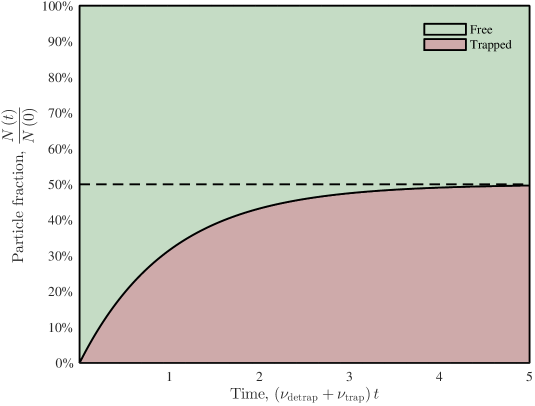
Figure 2: Free and trapped particle numbers for the exponential waiting time distribution $\phi\left(t\right)=\nu_{\mathrm{detrap}}\mathrm{e}^{-\nu_{\mathrm{detrap}}t}$. As no recombination is present, $\nu_{\mathrm{loss}}^{\left(\mathrm{free}\right)}=\nu_{\mathrm{loss}}^{\left(\mathrm{trap}\right)}=0$, an equilibrium steady state is reached between the particles as described by Eqs. (27) and (28). Here, the detrapping and trapping rates are set equal, $\nu_{\mathrm{detrap}}=\nu_{\mathrm{trap}}$, resulting in the same number of free and trapped particles in the steady state.

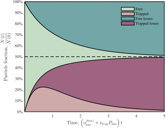
Figure 3: Free, trapped and recombined particle numbers for the exponential waiting time distribution $\phi\left(t\right)=\nu_{\mathrm{detrap}}\mathrm{e}^{-\nu_{\mathrm{detrap}}t}$. As recombination is present, all free and trapped particles are eventually lost in the proportions given by Eqs. (30) and (31). Transiently, however, there is an initial increase in the number of trapped particles. Here, we set equal the free particle recombination rate and the product of the trapping rate with the trapped particle recombination probability, $\nu_{\mathrm{loss}}^{\left(\mathrm{free}\right)}=\nu_{\mathrm{trap}}P_{\mathrm{loss}}$. For this exponential distribution of waiting times this probability is $P_{\mathrm{loss}}=\nu_{\mathrm{loss}}^{\left(\mathrm{trap}\right)}/\left(\nu_{\mathrm{detrap}}+\nu_{\mathrm{loss}}^{\left(\mathrm{trap}\right)}\right)$. By making the aforementioned quantities equal, the number of recombined free and trapped particles also become equal in the long time limit. In this case, the detrapping and trapping rates are set to $\nu_{\mathrm{detrap}}=\nu_{\mathrm{trap}}=\nu_{\mathrm{loss}}^{\left(\mathrm{free}\right)}+\nu_{\mathrm{trap}}P_{\mathrm{loss}}$, which consequently specifies the trapped particle recombination rate $\nu_{\mathrm{loss}}^{\left(\mathrm{trap}\right)}=\nu_{\mathrm{loss}}^{\left(\mathrm{free}\right)}+\nu_{\mathrm{trap}}P_{\mathrm{loss}}$.

III.3 Moments and transport coefficients

In this and later sections we will be predominantly interested in steady state quantities, independent of the choice of initial condition. For simplicity, we will assume there are initially $N\left(0\right)$ free particles centred at the origin with a Maxwellian distribution of velocities of temperature $T_{0}\equiv m/k_{\mathrm{B}}\alpha_{0}^{2}$

$$f\left(t=0,\mathbf{r},\mathbf{v}\right)\equiv N\left(0\right)\delta\left(\mathbf{r}\right)w\left(\alpha_{0},v\right).$$ (33)

Velocity integration of the generalised Boltzmann equation (1) provides the continuity equation for free particle number density

$$\left[\frac{\partial}{\partial t}+\nu_{\mathrm{trap}}\left(1-\Phi\left(t\right)\ast\right)+\nu_{\mathrm{loss}}^{\left(\mathrm{free}\right)}\right]n\left(t,\mathbf{r}\right)+\frac{\partial}{\partial\mathbf{r}}\cdot\left[n\left(t,\mathbf{r}\right)\left\langle\mathbf{v}\right\rangle\left(t,\mathbf{r}\right)\right]=0.$$ (34)

This can be solved analytically using the generalised Boltzmann equation solution (19), yielding

$$n\left(p,\mathbf{k}\right)=\frac{N\left(0\right)\zeta_{0}\left(\mathbf{k}\right)Z\left[-\left(\tilde{p}+\tilde{\nu}\right)\zeta_{0}\left(\mathbf{k}\right)\right]}{1-\nu_{\mathrm{coll}}\zeta_{\mathrm{coll}}\left(\mathbf{k}\right)Z\left[-\left(\tilde{p}+\tilde{\nu}\right)\zeta_{\mathrm{coll}}\left(\mathbf{k}\right)\right]-\nu_{\mathrm{trap}}\Phi\left(p\right)\zeta_{\mathrm{detrap}}\left(\mathbf{k}\right)Z\left[-\left(\tilde{p}+\tilde{\nu}\right)\zeta_{\mathrm{detrap}}\left(\mathbf{k}\right)\right]},$$ (35)

where the plasma dispersion function, $Z\left(\xi\right)$, is defined (Fried and Conte, 1961)

$$Z\left(\xi\right)\equiv\frac{1}{\sqrt{\pi}}\int_{-\infty}^{\infty}\mathrm{d}x\frac{\mathrm{e}^{-x^{2}}}{x-\xi},$$ (36)

and each Maxwellian yields a term of the form

$$\zeta\left(\mathbf{k}\right)\equiv\left[2\imath\mathbf{k}\cdot\left(\frac{\imath\mathbf{k}}{\alpha^{2}}-\mathbf{a}\right)\right]^{-\frac{1}{2}}.$$ (37)

From this analytical solution, phase-space averaged moments of the generalised Boltzmann equation can be found exactly for all times. For example, we have the spatial moments

$$\mathcal{L}\left\{\frac{N\left(t\right)}{N\left(0\right)}\left\langle\mathbf{r}\right\rangle\left(t\right)\right\} = \frac{\mathbf{a}}{\tilde{p}^{2}\left(\tilde{p}+\tilde{\nu}\right)},$$ (38)

$$\mathcal{L}\left\{\frac{N\left(t\right)}{N\left(0\right)}\left\langle\mathbf{r}\mathbf{r}\right\rangle\left(t\right)\right\} = \frac{2\mathbf{I}}{\tilde{p}^{2}\left(\tilde{p}+\tilde{\nu}\right)^{2}}\left[\frac{\tilde{p}}{\alpha_{0}^{2}}+\frac{\nu_{\mathrm{coll}}}{\alpha_{\mathrm{coll}}^{2}}+\frac{\nu_{\mathrm{trap}}\Phi\left(p\right)}{\alpha_{\mathrm{detrap}}^{2}}\right]+\frac{2\mathbf{a}\mathbf{a}}{\tilde{p}^{2}\left(\tilde{p}+\tilde{\nu}\right)^{2}}\left(\frac{1}{\tilde{p}}+\frac{2}{\tilde{p}+\tilde{\nu}}\right),$$

where the Laplace transform operator has been denoted explicitly here as $\mathcal{L}$. From these moments, the motion of the centre of mass (CM) can be described. The CM velocity is defined as the time rate of change of its position

$$\mathbf{W}_{\mathrm{CM}}\left(t\right)\equiv\frac{\mathrm{d}}{\mathrm{d}t}\left\langle\mathbf{r}\right\rangle\left(t\right),$$ (39)

while the CM diffusivity is defined as being proportional to the rate of change of particle dispersion about it

$$\mathbf{D}_{\mathrm{CM}}\left(t\right)\equiv\frac{1}{2}\frac{\mathrm{d}}{\mathrm{d}t}\left[\left\langle\mathbf{r}\mathbf{r}\right\rangle\left(t\right)-\left\langle\mathbf{r}\right\rangle\left(t\right)\left\langle\mathbf{r}\right\rangle\left(t\right)\right].$$ (40)

CM transport coefficients can be defined for the free, trapped and total particles. Although trapped particles are localised in space their CM still moves due to repeated detrapping and trapping.

The movement of the free particles can also be described by looking directly at velocity moments of the generalised Boltzmann equation (1)

$$\mathcal{L}\left\{\frac{N\left(t\right)}{N\left(0\right)}\left\langle\mathbf{v}\right\rangle\left(t\right)\right\} = \frac{\mathbf{a}}{\tilde{p}\left(\tilde{p}+\tilde{\nu}\right)},$$ (41)

$$\mathcal{L}\left\{\frac{N\left(t\right)}{N\left(0\right)}\left\langle\mathbf{r}\mathbf{v}\right\rangle\left(t\right)\right\} = \frac{\mathbf{I}}{\tilde{p}\left(\tilde{p}+\tilde{\nu}\right)^{2}}\left[\frac{\tilde{p}}{\alpha_{0}^{2}}+\frac{\nu_{\mathrm{coll}}}{\alpha_{\mathrm{coll}}^{2}}+\frac{\nu_{\mathrm{trap}}\Phi\left(p\right)}{\alpha_{\mathrm{detrap}}^{2}}\right]+\frac{\mathbf{a}\mathbf{a}}{\tilde{p}\left(\tilde{p}+\tilde{\nu}\right)^{2}}\left(\frac{1}{\tilde{p}}+\frac{2}{\tilde{p}+\tilde{\nu}}\right),$$ (42)

from which we define the average velocity

$$\mathbf{W}\left(t\right)\equiv\left\langle\mathbf{v}\right\rangle\left(t\right),$$ (43)

and average diffusivity

$$\mathbf{D}\left(t\right)\equiv\left\langle\mathbf{r}\mathbf{v}\right\rangle\left(t\right)-\left\langle\mathbf{r}\right\rangle\left(t\right)\left\langle\mathbf{v}\right\rangle\left(t\right).$$ (44)

Figure 4 plots the CM velocity $\mathbf{W}_{\mathrm{CM}}\left(t\right)$ for the free, trapped and total particles alongside the average velocity $\mathbf{W}\left(t\right)$ for the free particles. We can see that all measures of velocity begin at zero due to the Maxwellian initial condition (33) being spherically symmetric in velocity space. All velocities then increase due to the applied field, with the free particle CM velocity $\mathbf{W}_{\mathrm{CM}}^{\left(\mathrm{free}\right)}\left(t\right)$ and average velocity $\mathbf{W}\left(t\right)$ coinciding linearly at early times

$$\mathbf{W}\left(t\right)\approx\mathbf{W}_{\mathrm{CM}}^{\left(\mathrm{free}\right)}\left(t\right)\approx\mathbf{a}t.$$ (45)

A similar small time expansion can be written for the free particle diffusivites

$$\mathbf{D}\left(t\right)\approx\mathbf{D}_{\mathrm{CM}}^{\left(\mathrm{free}\right)}\left(t\right)\approx\frac{\mathbf{I}}{\alpha_{0}^{2}}t+\frac{\mathbf{a}\mathbf{a}}{12}\left[\nu_{\mathrm{coll}}+6\left(\nu_{\mathrm{loss}}^{\left(\mathrm{free}\right)}+\nu_{\mathrm{trap}}\right)\right]t^{4}.$$ (46)

This coincidence between the free particle CM and average velocities only lasts temporarily before the CM velocity decreases, becoming negative prior to reaching its positive steady state value. This movement of the free particle CM against the field is due to the processes of trapping and detrapping. Specifically, as all particles are initially untrapped, an unusually large "pulse" of particles are trapped near the origin, which is later released, causing a bias of the distribution and shifting the CM towards the origin. Similarly, as the diffusivity of particles trapped early is initially small, the free particle CM diffusivity $\mathbf{D}_{\mathrm{CM}}^{\left(\mathrm{free}\right)}\left(t\right)$ can also become transiently negative, as the distribution appears to "bunch up" near the origin as the initial pulse is released. Finally, we can see that all CM velocities approach the same steady state value, while the free particle average velocity approaches a separate steady state. Specifically, the CM transport coefficients, $\mathbf{W}_{\mathrm{CM}}\left(t\right)$ and $\mathbf{D}_{\mathrm{CM}}\left(t\right)$, approach the values given by Eqs. (83) and (84), while the average transport coefficients, $\mathbf{W}\left(t\right)$ and $\mathbf{D}\left(t\right)$, approach Eqs. (60) and (76).

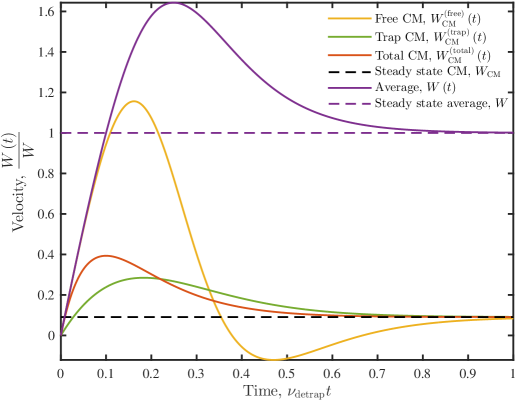
Figure 4: Plot of the centre of mass (CM) velocities for free, trapped and total particles, $\mathbf{W}_{\mathrm{CM}}^{\left(\mathrm{free}\right)}\left(t\right)$, $\mathbf{W}_{\mathrm{CM}}^{\left(\mathrm{trap}\right)}\left(t\right)$ and $\mathbf{W}_{\mathrm{CM}}^{\left(\mathrm{total}\right)}\left(t\right)$, as well as the actual average velocity for the free particles, $\mathbf{W}\left(t\right)$, for the exponential waiting time distribution $\phi\left(t\right)=\nu_{\mathrm{detrap}}\mathrm{e}^{-\nu_{\mathrm{detrap}}t}$. The free particle CM velocity $\mathbf{W}_{\mathrm{CM}}^{\left(\mathrm{free}\right)}\left(t\right)$ and average velocity $\mathbf{W}\left(t\right)$ coincide linearly at early times according to Eq. (45). The free particle CM velocity $\mathbf{W}_{\mathrm{CM}}\left(t\right)$ is seen to transiently become negative due to particles trapped early near the origin leaving their traps. In this case, there is no recombination present, $\nu_{\mathrm{loss}}^{\left(\mathrm{free}\right)}=\nu_{\mathrm{loss}}^{\left(\mathrm{trap}\right)}=0$, the collision frequency is set to $\nu_{\mathrm{coll}}/\nu_{\mathrm{detrap}}=1$ and the trapping rate is made sufficiently large so as the transient negative velocity manifests, $\nu_{\mathrm{trap}}/\nu_{\mathrm{detrap}}=10$. An additional consequence of this relatively large trapping rate is that almost all free particles become trapped early on, allowing the velocities to almost reach their steady state values after only a single trapping time $\nu_{\mathrm{detrap}}t=1$.

IV Hydrodynamic regime and the generalised diffusion equation

IV.1 Chapman-Enskog perturbative solution

The Chapman-Enskog perturbative solution technique (Chapman and Cowling, 1970) assumes that certain terms in the Boltzmann equation are small relative to others, allowing the solution to be written in the form of a Maclaurin series expansion. Traditionally, the Chapman-Enskog expansion assumes that both the explicit and implicit time derivatives in the Boltzmann equation are small. An implication of this is that the perturbative solution is valid only when the applied field is small. We will relax this condition and instead use a generalisation of the Chapman-Enskog expansion that only considers small explicit time and space derivatives, known as a hydrodynamic expansion. We expect the resulting solution to be most accurate in the long distance steady state. Note, however, in Subsection III.2 we determined that a steady state is not always attainable for our generalised Boltzmann equation (1). Specifically, if there is any recombination present, all free and trapped particles are eventually lost. To enforce that a steady state is always reached, we introduce the scaled phase-space distribution function of constant particle number $N\left(0\right)$

$$F\left(t,\mathbf{r},\mathbf{v}\right) \equiv \frac{N\left(0\right)}{N\left(t\right)}f\left(t,\mathbf{r},\mathbf{v}\right).$$ (47)

Substitution into the generalised Boltzmann equation (1) provides a corresponding generalised Boltzmann equation for this scaled distribution

$$\left(\frac{\partial}{\partial t}+\mathbf{v}\cdot\frac{\partial}{\partial\mathbf{r}}+\mathbf{a}\cdot\frac{\partial}{\partial\mathbf{v}}\right)F\left(t,\mathbf{r},\mathbf{v}\right)=-\nu_{\mathrm{coll}}\left[F\left(t,\mathbf{r},\mathbf{v}\right)-n_{F}\left(t,\mathbf{r}\right)w\left(\alpha_{\mathrm{coll}},v\right)\right]\\ -\nu_{\mathrm{trap}}\left[R\left(t\right)F\left(t,\mathbf{r},\mathbf{v}\right)-R\left(t,\mathbf{r}\right)n_{F}\left(t,\mathbf{r}\right)w\left(\alpha_{\mathrm{detrap}},v\right)\right],$$ (48)

where $n_{F}\left(t,\mathbf{r}\right)\equiv\int\mathrm{d}\mathbf{v}F\left(t,\mathbf{r},\mathbf{v}\right)$ and we have introduced the ratio of detrapping and trapping rates

$$R\left(t,\mathbf{r}\right)\equiv\frac{\Phi\left(t\right)\ast n\left(t,\mathbf{r}\right)}{n\left(t,\mathbf{r}\right)},$$ (49)

and its spatially homogeneous form

$$R\left(t\right)\equiv\frac{\Phi\left(t\right)\ast N\left(t\right)}{N\left(t\right)}.$$ (50)

On the terms we wish to denote as small, we will temporarily introduce a multiplicative parameter $\delta$

$$\delta\left(\frac{\partial}{\partial t}+\mathbf{v}\cdot\frac{\partial}{\partial\mathbf{r}}\right)F_{\delta}\left(t,\mathbf{r},\mathbf{v}\right)+\mathbf{a}\cdot\frac{\partial}{\partial\mathbf{v}}F_{\delta}\left(t,\mathbf{r},\mathbf{v}\right)=-\nu_{\mathrm{coll}}\left[F_{\delta}\left(t,\mathbf{r},\mathbf{v}\right)-n_{F}\left(t,\mathbf{r}\right)w\left(\alpha_{\mathrm{coll}},v\right)\right]\\ -\nu_{\mathrm{trap}}\left[R\left(t\right)F_{\delta}\left(t,\mathbf{r},\mathbf{v}\right)-R\left(t,\mathbf{r}\right)n_{F}\left(t,\mathbf{r}\right)w\left(\alpha_{\mathrm{detrap}},v\right)\right],$$ (51)

through which we can expand the solution in a power series

$$F_{\delta}\left(t,\mathbf{r},\mathbf{v}\right)=\sum_{n\geq 0}F^{\left(n\right)}\left(t,\mathbf{r},\mathbf{v}\right)\delta^{n}.$$ (52)

This allows the actual solution to be recovered by setting $\delta=1$ in the above series expansion

$$F\left(t,\mathbf{r},\mathbf{v}\right)=\sum_{n\geq 0}F^{\left(n\right)}\left(t,\mathbf{r},\mathbf{v}\right).$$ (53)

The terms in this series solution can be found recursively by substituting the $\delta$ expansion (52) for $F_{\delta}\left(t,\mathbf{r},\mathbf{v}\right)$ into the generalised Boltzmann equation (51) and equating powers of $\delta$

$$\left[\nu_{\mathrm{coll}}+\nu_{\mathrm{trap}}R\left(t\right)+\mathbf{a}\cdot\frac{\partial}{\partial\mathbf{v}}\right]F^{\left(n\right)}\left(t,\mathbf{r},\mathbf{v}\right)=-\left(\frac{\partial}{\partial t}+\mathbf{v}\cdot\frac{\partial}{\partial\mathbf{r}}\right)F^{\left(n-1\right)}\left(t,\mathbf{r},\mathbf{v}\right).$$ (54)

This recurrence relationship is valid for $n\geq 1$, with the initial term given separately as

$$\left[1+\left\langle\mathbf{v}\right\rangle^{\left(0\right)}\left(t\right)\cdot\frac{\partial}{\partial\mathbf{v}}\right]F^{\left(0\right)}\left(t,\mathbf{r},\mathbf{v}\right)=\frac{\nu_{\mathrm{coll}}w\left(\alpha_{\mathrm{coll}},v\right)+\nu_{\mathrm{trap}}R\left(t,\mathbf{r}\right)w\left(\alpha_{\mathrm{detrap}},v\right)}{\nu_{\mathrm{coll}}+\nu_{\mathrm{trap}}R\left(t,\mathbf{r}\right)}n_{F}\left(t,\mathbf{r}\right),$$ (55)

in terms of its average velocity

$$\left\langle\mathbf{v}\right\rangle^{\left(0\right)}\left(t\right)\equiv\frac{\mathbf{a}}{\nu_{\mathrm{coll}}+\nu_{\mathrm{trap}}R\left(t\right)}.$$ (56)

Note here we have enforced the normalisation condition

$$\int\mathrm{d}\mathbf{v}F^{\left(0\right)}\left(t,\mathbf{r},\mathbf{v}\right)\equiv n_{F}\left(t,\mathbf{r}\right).$$ (57)

In Fourier-transformed velocity space we can write this initial term explicitly

$$F^{\left(0\right)}\left(t,\mathbf{r},\mathbf{s}\right)=\tilde{w}\left(t,\mathbf{r},\mathbf{s}\right)n_{F}\left(t,\mathbf{r}\right),$$ (58)

where

$$\tilde{w}\left(t,\mathbf{r},\mathbf{s}\right)\equiv\frac{1}{1+\left\langle\mathbf{v}\right\rangle^{\left(0\right)}\left(t\right)\cdot\imath\mathbf{s}}\frac{\nu_{\mathrm{coll}}w\left(\alpha_{\mathrm{coll}},s\right)+\nu_{\mathrm{trap}}R\left(t,\mathbf{r}\right)w\left(\alpha_{\mathrm{detrap}},s\right)}{\nu_{\mathrm{coll}}+\nu_{\mathrm{trap}}R\left(t,\mathbf{r}\right)}.$$ (59)

We can confirm that this approximate hydrodynamic solution is most accurate in the steady state by noting that its average velocity coincides with the actual average velocity (43) at late times, $\lim_{t\rightarrow\infty}\left\langle\mathbf{v}\right\rangle^{\left(0\right)}\left(t\right)=\lim_{t\rightarrow\infty}\left\langle\mathbf{v}\right\rangle\left(t\right)$. We will denote this shared steady state velocity as

$$\mathbf{W}\equiv\frac{\mathbf{a}}{\nu_{\mathrm{eff}}},$$ (60)

where the separate collision and trapping processes contribute to the effective frequency

$$\nu_{\mathrm{eff}}\equiv\nu_{\mathrm{coll}}+R\nu_{\mathrm{trap}},$$ (61)

defined in terms of the spatially averaged limiting ratio of detrapping and trapping rates

$$R\equiv\lim_{t\rightarrow\infty}R\left(t\right).$$ (62)

This limit can be evaluated implicitly as satisfying

$$R\equiv\int_{0}^{\infty}\mathrm{d}t\Phi\left(t\right)\mathrm{e}^{\left[\nu_{\mathrm{loss}}^{\left(\mathrm{free}\right)}+\nu_{\mathrm{trap}}\left(1-R\right)\right]t}.$$ (63)

Specific expressions for $R$ for various choices of the waiting time distribution $\phi\left(t\right)$ are listed in Appendix A. In terms of this velocity, $\mathbf{W}$, we can write the steady state limit of Eq. (59) as

$$\tilde{w}\left(\mathbf{r},\mathbf{s}\right)=\frac{1}{1+\mathbf{W}\cdot\imath\mathbf{s}}\frac{\nu_{\mathrm{coll}}w\left(\alpha_{\mathrm{coll}},s\right)+\nu_{\mathrm{trap}}R\left(\mathbf{r}\right)w\left(\alpha_{\mathrm{detrap}},s\right)}{\nu_{\mathrm{coll}}+\nu_{\mathrm{trap}}R\left(\mathbf{r}\right)},$$ (64)

where the limiting ratio of detrapping and trapping rates is

$$R\left(\mathbf{r}\right)\equiv\lim_{t\rightarrow\infty}R\left(t,\mathbf{r}\right).$$ (65)

In direct analogy with the implicit definition (63) of $R$ we have the following implicit definition of $R\left(\mathbf{r}\right)$

$$R\left(\mathbf{r}\right)\equiv\int_{0}^{\infty}\mathrm{d}t\Phi\left(t\right)\exp\left\{\left[\nu_{\mathrm{loss}}^{\left(\mathrm{free}\right)}+\nu_{\mathrm{trap}}\left(1-R\left(\mathbf{r}\right)\right)+\frac{1}{n}\frac{\partial}{\partial\mathbf{r}}\cdot n\left\langle\mathbf{v}\right\rangle\right]t\right\}.$$ (66)

Finally, we can explore the spatial dependence of $\tilde{w}\left(\mathbf{r},\mathbf{s}\right)$ by considering a perturbation from its spatially averaged state

$$\tilde{w}\left(\mathbf{s}\right)=\frac{\nu_{\mathrm{coll}}w\left(\alpha_{\mathrm{coll}},s\right)+\nu_{\mathrm{trap}}Rw\left(\alpha_{\mathrm{detrap}},s\right)}{\nu_{\mathrm{coll}}+\nu_{\mathrm{trap}}R+\mathbf{a}\cdot\imath\mathbf{s}}.$$ (67)

To spatially perturb $\tilde{w}\left(\mathbf{s}\right)$, we must first spatially perturb $R$ using the definition (66) of $R\left(\mathbf{r}\right)$. Introducing the first order spatial perturbation $\delta R$ and using the asymptotic velocity in the hydrodynamic regime, $\left\langle\mathbf{v}\right\rangle\sim\mathbf{W}$, provides the expression

$$R+\delta R=R\left\langle\exp\left[\left(\frac{1}{n}\frac{\partial n}{\partial\mathbf{r}}\cdot\mathbf{W}-\nu_{\mathrm{trap}}\delta R\right)t\right]\right\rangle,$$ (68)

in terms of the time average defined by

$$\left\langle\eta\left(t\right)\right\rangle\equiv\frac{1}{R}\int_{0}^{\infty}\mathrm{d}t\Phi\left(t\right)\mathrm{e}^{\left[\nu_{\mathrm{loss}}^{\left(\mathrm{free}\right)}+\nu_{\mathrm{trap}}\left(1-R\right)\right]t}\eta\left(t\right).$$ (69)

Performing a power series expansion and truncating beyond first order gives the solution $R\left(\mathbf{r}\right)=R+\delta R$ as a density gradient expansion up to first order

$$R\left(\mathbf{r}\right)=R+\mathbf{R}^{\left(1\right)}\cdot\frac{1}{n}\frac{\partial n}{\partial\mathbf{r}},$$ (70)

in terms of the vector coefficient

$$\mathbf{R}^{\left(1\right)}\equiv\frac{R\left\langle t\right\rangle}{1+\nu_{\mathrm{trap}}R\left\langle t\right\rangle}\mathbf{W}.$$ (71)

Now the spatially averaged steady state velocity distribution $\tilde{w}\left(\mathbf{s}\right)$ can be spatially perturbed using the density gradient expansion (70), resulting in, to first spatial order

$$F^{\left(0\right)}\left(t,\mathbf{r},\mathbf{s}\right) = \tilde{w}\left(\mathbf{s}\right)n_{F}\left(t,\mathbf{r}\right)$$ (72)

$$+\frac{w\left(\alpha_{\mathrm{detrap}},s\right)-\tilde{w}\left(\mathbf{s}\right)}{\nu_{\mathrm{coll}}+\nu_{\mathrm{trap}}R+\mathbf{a}\cdot\imath\mathbf{s}}\nu_{\mathrm{trap}}\mathbf{R}^{\left(1\right)}\cdot\frac{\partial}{\partial\mathbf{r}}n_{F}\left(t,\mathbf{r}\right).$$

Using the recurrence relationship (54) and the continuity equation (34) to evaluate the explicit time derivative provides the next term, also to first spatial order

$$F^{\left(1\right)}\left(t,\mathbf{r},\mathbf{s}\right) = \frac{\mathbf{W}\tilde{w}\left(\mathbf{s}\right)-\imath\frac{\partial}{\partial\mathbf{s}}\tilde{w}\left(\mathbf{s}\right)}{\nu_{\mathrm{coll}}+\nu_{\mathrm{trap}}R+\mathbf{a}\cdot\imath\mathbf{s}}\cdot\frac{\partial}{\partial\mathbf{r}}n_{F}\left(t,\mathbf{r}\right).$$ (73)

Similarly, $F^{\left(2\right)}\left(t,\mathbf{r},\mathbf{v}\right)$ can be found and shown to be of minimum second order in spatial gradients. In general, $F^{\left(n\right)}\left(t,\mathbf{r},\mathbf{v}\right)$ is described by a full density gradient expansion of minimum spatial order $n$. Including all zeroth and first order contributions, the generalised Boltzmann equation solution is

$$f\left(t,\mathbf{r},\mathbf{s}\right) = \tilde{w}\left(\mathbf{s}\right)n\left(t,\mathbf{r}\right)$$ (74)

$$+\frac{\left[\mathbf{W}-\nu_{\mathrm{trap}}\mathbf{R}^{\left(1\right)}-\imath\frac{\partial}{\partial\mathbf{s}}\right]\tilde{w}\left(\mathbf{s}\right)+\nu_{\mathrm{trap}}\mathbf{R}^{\left(1\right)}w\left(\alpha_{\mathrm{detrap}},s\right)}{\nu_{\mathrm{coll}}+\nu_{\mathrm{trap}}R+\mathbf{a}\cdot\imath\mathbf{s}}\cdot\frac{\partial}{\partial\mathbf{r}}n\left(t,\mathbf{r}\right).$$

Velocity integration provides Fick’s law for the free particle flux

$$n\left\langle\mathbf{v}\right\rangle=\mathbf{W}n-\mathbf{D}\cdot\frac{\partial n}{\partial\mathbf{r}},$$ (75)

which implies that $\mathbf{W}$ is the flux drift velocity and defines the flux diffusion coefficient as

$$\mathbf{D}\equiv\frac{1}{\nu_{\mathrm{eff}}}\left[\frac{\mathbf{I}}{\alpha_{\mathrm{eff}}^{2}}+\left(\mathbf{W}+\nu_{\mathrm{trap}}\mathbf{R}^{\left(1\right)}\right)\mathbf{W}\right],$$ (76)

written in terms of the effective frequency (61) and the effective temperature

$$T_{\mathrm{eff}} \equiv \frac{\nu_{\mathrm{coll}}}{\nu_{\mathrm{coll}}+R\nu_{\mathrm{trap}}}T_{\mathrm{coll}}+\frac{R\nu_{\mathrm{trap}}}{\nu_{\mathrm{coll}}+R\nu_{\mathrm{trap}}}T_{\mathrm{detrap}}.$$ (77)

Similar to the flux drift velocity $\mathbf{W}$, the flux diffusion coefficient $\mathbf{D}$ could have also been derived as the long time limit of the average diffusivity (44)

$$\mathbf{D}\equiv\lim_{t\rightarrow\infty}\left[\left\langle\mathbf{r}\mathbf{v}\right\rangle\left(t\right)-\left\langle\mathbf{r}\right\rangle\left(t\right)\left\langle\mathbf{v}\right\rangle\left(t\right)\right].$$ (78)

The flux diffusion coefficient derived here differs slightly from what was derived in (Philippa et al., 2014) for a similar phase-space kinetic model utilising the same operator for trapping and detrapping. It is likely they did not consider the spatial dependence in Eq. (49) for the ratio of detrapping and trapping rates $R\left(t,\mathbf{r}\right)$, as their diffusion coefficient lacked the additional anisotropic component $\frac{\nu_{\mathrm{trap}}}{\nu_{\mathrm{eff}}}\mathbf{R}^{\left(1\right)}\mathbf{W}$. Subsequently, their diffusion coefficient is only valid in the isotropic case without an applied field, where $\mathbf{W}=0$, or in the limit of instantaneous detrapping, where $\mathbf{R}^{\left(1\right)}=\mathbf{0}$.

IV.2 Analytical correspondence of transport coefficients

IV.2.1 Diffusion equations in the hydrodynamic regime

In the previous subsection we considered a perturbative solution of the generalised Boltzmann equation (1), written in the hydrodynamic regime as the density gradient expansion (74). This solution directly provided the flux transport coefficients of velocity (60) and diffusion (76). In this subsection, we look to reconcile these results analytically using Eq. (35) for the number density. We can describe the asymptotics of the number density by looking at its poles in Laplace space, given by solving the dispersion relation (Robson, 1975)

$$1-\nu_{\mathrm{coll}}\zeta_{\mathrm{coll}}\left(\mathbf{k}\right)Z\left[-\left(\tilde{p}+\tilde{\nu}\right)\zeta_{\mathrm{coll}}\left(\mathbf{k}\right)\right]-\nu_{\mathrm{trap}}\Phi\left(p\right)\zeta_{\mathrm{detrap}}\left(\mathbf{k}\right)Z\left[-\left(\tilde{p}+\tilde{\nu}\right)\zeta_{\mathrm{detrap}}\left(\mathbf{k}\right)\right]=0.$$ (79)

Using the asymptotic series representation of the plasma dispersion function (Fried and Conte, 1961)

$$Z\left(\xi\right)=-\frac{1}{\xi}\sum_{n\geq 0}\frac{\left(2n-1\right)!!}{2^{n}}\xi^{-2n}=-\frac{1}{\xi}\left(1+\frac{1}{2}\xi^{-2}+\frac{3}{4}\xi^{-4}+\cdots\right),$$ (80)

we perform a small $\mathbf{k}$ expansion and find the root of the dispersion relation to second spatial order

$$p=-\nu_{\mathrm{trap}}\left(1-R\right)-\nu_{\mathrm{loss}}^{\left(\mathrm{free}\right)}-\mathbf{W}_{\mathrm{CM}}\cdot\imath\mathbf{k}+\mathbf{D}_{\mathrm{CM}}\colon\imath\mathbf{k}\imath\mathbf{k},$$ (81)

which corresponds to the diffusion equation

$$\left[\frac{\partial}{\partial t}+\nu_{\mathrm{trap}}\left(1-R\right)+\nu_{\mathrm{loss}}^{\left(\mathrm{free}\right)}+\mathbf{W}_{\mathrm{CM}}\cdot\frac{\partial}{\partial\mathbf{r}}-\mathbf{D}_{\mathrm{CM}}\colon\frac{\partial^{2}}{\partial\mathbf{r}\partial\mathbf{r}}\right]n\left(t,\mathbf{r}\right)=0.$$ (82)

Here the steady state centre of mass (CM) transport coefficients are defined

$$\mathbf{W}_{\mathrm{CM}} \equiv \frac{\mathbf{R}^{\left(1\right)}}{R\left\langle t\right\rangle},$$ (83)

$$\mathbf{D}_{\mathrm{CM}} \equiv \frac{\left\langle t^{2}\right\rangle}{2\left\langle t\right\rangle}\mathbf{W}_{\mathrm{CM}}\mathbf{W}_{\mathrm{CM}}-\frac{\mathbf{R}^{\left(2\right)}}{R\left\langle t\right\rangle},$$ (84)

using the density gradient expansion of $R\left(\mathbf{r}\right)$

$$R\left(\mathbf{r}\right)=R+\mathbf{R}^{\left(1\right)}\cdot\frac{1}{n}\frac{\partial n}{\partial\mathbf{r}}+\mathbf{R}^{\left(2\right)}\colon\frac{1}{n}\frac{\partial^{2}n}{\partial\mathbf{r}\partial\mathbf{r}},$$ (85)

written now to second order using the flux diffusion coefficient $\mathbf{D}$

$$\mathbf{R}^{\left(2\right)}\equiv\frac{R\left\langle t^{2}\right\rangle}{2\left(1+\nu_{\mathrm{trap}}R\left\langle t\right\rangle\right)^{3}}\mathbf{W}\mathbf{W}-\frac{R\left\langle t\right\rangle}{1+\nu_{\mathrm{trap}}R\left\langle t\right\rangle}\mathbf{D},$$ (86)

where time averages are defined by Eq. (69). Substitution of the root of the dispersion relation into the time operator of the continuity equation yields, to second spatial order

$$p+\nu_{\mathrm{trap}}\left[1-\Phi\left(p\right)\right]+\nu_{\mathrm{loss}}^{\left(\mathrm{free}\right)}=-\mathbf{W}\cdot\imath\mathbf{k}+\mathbf{D}\colon\imath\mathbf{k}\imath\mathbf{k},$$ (87)

which corresponds to the generalised diffusion equation

$$\left[\frac{\partial}{\partial t}+\nu_{\mathrm{trap}}\left(1-\Phi\left(t\right)\ast\right)+\nu_{\mathrm{loss}}^{\left(\mathrm{free}\right)}+\mathbf{W}\cdot\frac{\partial}{\partial\mathbf{r}}-\mathbf{D}\colon\frac{\partial^{2}}{\partial\mathbf{r}\partial\mathbf{r}}\right]n\left(t,\mathbf{r}\right)=0,$$ (88)

in terms of the flux transport coefficients $\mathbf{W}$ and $\mathbf{D}$. This could have alternatively been derived by approximating the flux in the continuity equation directly using its density gradient expansion (Fick’s law) given by Eq. (75).

IV.2.2 Approaching the steady state

So far we have considered the continuity equation in both the steady and near spatially homogeneous state. Using the analytical solution, it is possible to relax this steady state assumption. We can write the flux exactly by rearranging the continuity equation (34) in Fourier-Laplace space

$$\imath\mathbf{k}\cdot\mathcal{L}\left\{n\left(t,\mathbf{k}\right)\left\langle\mathbf{v}\right\rangle\left(t\right)\right\}=\left[\frac{N\left(0\right)}{n\left(p,\mathbf{k}\right)}-\tilde{p}\right]n\left(p,\mathbf{k}\right).$$ (89)

Performing a small $\mathbf{k}$ expansion of the above coefficient of $n\left(p,\mathbf{k}\right)$ gives an approximate continuity equation valid for large distances or near spatially homogeneous states

$$\left[p+\nu_{\mathrm{trap}}\left(1-\Phi\left(p\right)\right)+\nu_{\mathrm{loss}}^{\left(\mathrm{free}\right)}+\boldsymbol{\mathfrak{W}}\left(p\right)\cdot\imath\mathbf{k}-\boldsymbol{\mathfrak{D}}\left(p\right)\colon\imath\mathbf{k}\imath\mathbf{k}\right]n\left(p,\mathbf{k}\right)=N\left(0\right),$$ (90)

where the following $p$-dependent velocity and diffusivity are defined in Laplace space

$$\boldsymbol{\mathfrak{W}}\left(p\right) \equiv \frac{\mathbf{a}}{\tilde{p}+\tilde{\nu}},$$ (91)

$$\boldsymbol{\mathfrak{D}}\left(p\right) \equiv \frac{\mathbf{I}}{\left(\tilde{p}+\tilde{\nu}\right)^{2}}\left[\frac{\tilde{p}}{\alpha_{0}^{2}}+\frac{\nu_{\mathrm{coll}}}{\alpha_{\mathrm{coll}}^{2}}+\frac{\nu_{\mathrm{trap}}\Phi\left(p\right)}{\alpha_{\mathrm{detrap}}^{2}}\right]+\frac{2\mathbf{a}\mathbf{a}}{\left(\tilde{p}+\tilde{\nu}\right)^{3}},$$ (92)

although in the time domain $\boldsymbol{\mathfrak{W}}\left(t\right)$ and $\boldsymbol{\mathfrak{D}}\left(t\right)$ have units of length and area respectively. Performing the inverse Fourier-Laplace transform yields

$$\left[\frac{\partial}{\partial t}+\nu_{\mathrm{trap}}\left(1-\Phi\left(t\right)\ast\right)+\nu_{\mathrm{loss}}^{\left(\mathrm{free}\right)}+\boldsymbol{\mathfrak{W}}\left(t\right)\ast\cdot\frac{\partial}{\partial\mathbf{r}}-\boldsymbol{\mathfrak{D}}\left(t\right)\ast\colon\frac{\partial^{2}}{\partial\mathbf{r}\partial\mathbf{r}}\right]n\left(t,\mathbf{r}\right)=0,$$ (93)

which is of a similar form to the generalised diffusion equation, but now the “transport coefficients” are time convolved with the number density. It should be noted that, as the flux has been written to second spatial order, the first and second order spatial moments of this approximate continuity equation are exact for all times.

V Connection with fractional transport

Dispersive transport is physically characterised by long-lived traps (Scher and Montroll, 1975). For the right choice of parameters, the generalised Boltzmann equation (1) is capable of modelling such trapped states. A necessary condition for dispersive transport is a waiting time distribution with a divergent mean. One choice is a waiting time distribution with a heavy tail of the power law form

$$\phi\left(t\right)\sim t^{-\left(1+\alpha\right)},$$ (94)

where $0<\alpha<1$. This takes the small $p$ form in Laplace space

$$\phi\left(p\right)\approx 1-r_{\alpha}p^{\alpha}.$$ (95)

Additionally, we must enforce that no trap-based recombination occurs, $\nu_{\mathrm{loss}}^{\left(\mathrm{trap}\right)}=0$, as this has the effect of prematurely shortening the trapping time so that the mean trapping time no longer diverges. In this case, the effective waiting time distribution (5) is no longer weighted by an exponential decay term, $\Phi\left(t\right)\rightarrow\phi\left(t\right)$, and the continuity equation (34) becomes

$$\left[\frac{\partial}{\partial t}+\nu_{\mathrm{trap}}\left(1-\phi\left(t\right)\ast\right)+\nu_{\mathrm{loss}}^{\left(\mathrm{free}\right)}\right]n\left(t,\mathbf{r}\right)+\frac{\partial}{\partial\mathbf{r}}\cdot\left[n\left(t,\mathbf{r}\right)\left\langle\mathbf{v}\right\rangle\left(t,\mathbf{r}\right)\right]=0.$$ (96)

We can separate the power law tail from the waiting time distribution

$$\phi\left(t\right)\ast n\left(t,\mathbf{r}\right)=\psi\left(t\right)\ast n\left(t,\mathbf{r}\right)-r_{\alpha}\left[{}_{0}^{\mathrm{C}}\mathcal{D}_{t}^{\alpha}n\left(t,\mathbf{r}\right)+\frac{t^{-\alpha}}{\Gamma\left(1-\alpha\right)}n\left(0,\mathbf{r}\right)\right],$$ (97)

where the moments of $\psi\left(t\right)$ are well-defined and the operator of Caputo fractional differentiation of order $\alpha$ is defined

$${}_{0}^{\mathrm{C}}\mathcal{D}_{t}^{\alpha}n\left(t,\mathbf{r}\right)\equiv\frac{1}{\Gamma\left(1-\alpha\right)}\int_{0}^{t}\mathrm{d}\tau\left(t-\tau\right)^{-\alpha}\frac{\partial}{\partial\tau}n\left(\tau,\mathbf{r}\right).$$ (98)

The continuity equation can now be written exactly as

$$\left[\frac{\partial}{\partial t}+r_{\alpha}\nu_{\mathrm{trap}}{}_{0}^{\mathrm{C}}\mathcal{D}_{t}^{\alpha}+\nu_{\mathrm{trap}}\left(1-\psi\left(t\right)\ast\right)+\nu_{\mathrm{loss}}^{\left(\mathrm{free}\right)}\right]n\left(t,\mathbf{r}\right)+\frac{\partial}{\partial\mathbf{r}}\cdot\left[n\left(t,\mathbf{r}\right)\left\langle\mathbf{v}\right\rangle\left(t,\mathbf{r}\right)\right]=-\frac{r_{\alpha}\nu_{\mathrm{trap}}}{t^{\alpha}\Gamma\left(1-\alpha\right)}n\left(0,\mathbf{r}\right).$$ (99)

Truncating the small $p$ expansion in Laplace space yields a form of the continuity equation valid for long times

$$\left({}_{0}^{\mathrm{C}}\mathcal{D}_{t}^{\alpha}+\frac{\nu_{\mathrm{loss}}^{\left(\mathrm{free}\right)}}{r_{\alpha}\nu_{\mathrm{trap}}}\right)n\left(t,\mathbf{r}\right)+\frac{\partial}{\partial\mathbf{r}}\cdot\left[n\left(t,\mathbf{r}\right)\frac{\left\langle\mathbf{v}\right\rangle\left(t,\mathbf{r}\right)}{r_{\alpha}\nu_{\mathrm{trap}}}\right]=\left[\delta\left(r_{\alpha}\nu_{\mathrm{trap}}t\right)-\frac{t^{-\alpha}}{\Gamma\left(1-\alpha\right)}\right]n\left(0,\mathbf{r}\right),$$ (100)

written now solely in terms of the time operator of fractional differentiation. Finally, performing a small $\mathbf{k}$ approximation in Fourier space provides the Captuo time-fractional advection-diffusion equation

$$\left({}_{0}^{\mathrm{C}}\mathcal{D}_{t}^{\alpha}+\frac{\nu_{\mathrm{loss}}^{\left(\mathrm{free}\right)}}{r_{\alpha}\nu_{\mathrm{trap}}}+\mathbf{W}_{\alpha}\cdot\frac{\partial}{\partial\mathbf{r}}-\mathbf{D}_{\alpha}\cdot\frac{\partial^{2}}{\partial\mathbf{r}\partial\mathbf{r}}\right)n\left(t,\mathbf{r}\right)=\left[\delta\left(r_{\alpha}\nu_{\mathrm{trap}}t\right)-\frac{t^{-\alpha}}{\Gamma\left(1-\alpha\right)}\right]n\left(0,\mathbf{r}\right),$$ (101)

with fractional transport coefficients defined as

$$\mathbf{W}_{\alpha} \equiv \frac{\mathbf{W}}{\nu_{\mathrm{trap}}r_{\alpha}},$$ (102)

$$\mathbf{D}_{\alpha} \equiv \frac{\mathbf{D}}{\nu_{\mathrm{trap}}r_{\alpha}},$$ (103)

in terms of the flux drift velocity (60) and diffusion coefficient (76), respectively. Note that, as the waiting time distribution $\phi\left(t\right)$ has a divergent mean, the flux diffusion coefficient takes the particular form

$$\mathbf{D}\equiv\frac{1}{\nu_{\mathrm{eff}}}\left(\frac{\mathbf{I}}{\alpha_{\mathrm{eff}}^{2}}+2\mathbf{W}\mathbf{W}\right).$$ (104)

There exist generalisations of time-fractional diffusion equations, like Eq. (101), where spatial derivatives are also taken to be of non-integer order (Mainardi et al., 2001). Physically, these fractional space derivatives arise when particles undergo long jumps in space (Metzler and Klafter, 2004). This is analogous to the above situation where a time-fractional diffusion equation arose from particles experiencing traps of long duration. As our model currently only allows for variation in the trapping time, we conclude that to similarly derive a space-fractional diffusion equation would require adjustments to the kinetic theory.

Importantly, we should also note that a similar asymptotic approximation of the generalised Boltzmann equation (1) does not result in a fractional time operator that acts on the phase-space distribution function. That is, it does not seem possible to derive a similar “fractional Boltzmann equation” from our model. This conclusion differs from (Robson and Blumen, 2005) who used a similar kinetic model to successfully derive a fractional Boltzmann equation. However, their model was inconsistent as it simultaneously modelled trapping while also maintaining a constant number of free particles.

VI Subordination transformation

As shown in the previous section, the generalised diffusion equation is capable of describing dispersive transport in the same way the Caputo fractional diffusion equation does. A general feature shared by both of these diffusion equations is the history dependence of their solutions. This is physically due to the existence of trapped states and delayed detrapping. Mathematically, this manifests as a global time operator, be it a fractional derivative or, in the case of the generalised diffusion equation (88), a convolution with the effective waiting time distribution $\Phi\left(t\right)$.

Due to their nature, global operators introduce additional complexity when it comes to solving problems numerically. For example, in finite difference schemes the computation time generally scales linearly with the number of time steps chosen. The exception being when a global time operator is present, causing the computation time to scale quadratically with the number of time steps. Although this increased computational complexity is inherent to these systems, a number of techniques have been suggested to improve upon it for fractional differential equations (Podlubny, 1998; Ford and Simpson, 2001; Fukunaga and Shimizu, 2011; Stokes et al., 2015). One approach involves first solving a standard diffusion equation and then performing a subordination integral transformation (Barkai, 2001; Stokes et al., 2015) to find the desired solution of a fractional diffusion equation. We will generalise this approach to solve the generalised diffusion equation for the free particle number density $n\left(t,\mathbf{r}\right)$.

Replacing the time operator in the generalised diffusion equation with an explicit time derivative yields a standard diffusion equation with the same linear spatial operator

$$\left(\frac{\partial}{\partial\tau}+\mathbf{W}\cdot\frac{\partial}{\partial\mathbf{r}}-\mathbf{D}\colon\frac{\partial^{2}}{\partial\mathbf{r}\partial\mathbf{r}}\right)u\left(\tau,\mathbf{r}\right)=0.$$ (105)

For the same initial conditions, $u\left(0,\mathbf{r}\right)\equiv n\left(0,\mathbf{r}\right)$, we can relate both solutions directly in Laplace space

$$n\left(p,\mathbf{r}\right)=u\left(p+\nu_{\mathrm{loss}}^{\left(\mathrm{free}\right)}+\nu_{\mathrm{trap}}\left[1-\Phi\left(p\right)\right],\mathbf{r}\right),$$ (106)

which in the time domain corresponds to the subordination integral transform

$$n\left(t,\mathbf{r}\right) \equiv \mathcal{A}u\left(t,\mathbf{r}\right)$$ (107)

$$\equiv \int_{0}^{t}\mathrm{d}\tau A\left(\tau,t-\tau\right)u\left(\tau,\mathbf{r}\right),$$

where the kernel is defined in terms of the inverse Laplace transform $\mathcal{L}^{-1}$

$$A\left(\tau,t\right)\equiv\mathrm{e}^{-\left(\nu_{\mathrm{loss}}^{\left(\mathrm{free}\right)}+\nu_{\mathrm{trap}}\right)\tau}\mathrm{e}^{-\nu_{\mathrm{loss}}^{\left(\mathrm{trap}\right)}t}\mathcal{L}^{-1}\left\{e^{\nu_{\mathrm{trap}}\phi\left(p\right)\tau}\right\}.$$ (108)

Appendix B contains kernels corresponding to various choices of the waiting time distribution $\phi\left(t\right)$.

As a simple example, consider the case of a shifted Dirac delta waiting time distribution

$$\phi\left(t\right)=\delta\left(t-\nu_{\mathrm{detrap}}^{-1}\right),$$ (109)

corresponding to traps of fixed duration $\nu_{\mathrm{detrap}}^{-1}$. In this case, the subordination transformation (107) simply becomes the summation

$$n\left(t,\mathbf{r}\right)=\sum_{k\geq 0}n^{\left(k\right)}\left(t-k\nu_{\mathrm{detrap}}^{-1},\mathbf{r}\right),$$ (110)

the terms of which can be physically interpreted as those free particles which have been trapped $k$ times in the past

$$n^{\left(k\right)}\left(\tau,\mathbf{r}\right)\equiv H\left(\tau\right)\frac{\left(\mathrm{e}^{-\frac{\nu_{\mathrm{loss}}^{\left(\mathrm{trap}\right)}}{\nu_{\mathrm{detrap}}}}\nu_{\mathrm{trap}}\tau\right)^{k}}{k!}\mathrm{e}^{-\left(\nu_{\mathrm{loss}}^{\left(\mathrm{free}\right)}+\nu_{\mathrm{trap}}\right)\tau}u\left(\tau,\mathbf{r}\right),$$ (111)

where $H\left(\tau\right)$ is the Heaviside step function. Figure 5 plots this solution on a one-dimensional unbounded domain $z\in\left(-\infty,\infty\right)$ for the impulse initial condition $n\left(0,z\right)\equiv N\left(0\right)\delta\left(z\right)$, and shows its construction in terms of the corresponding Gaussian solution of the standard diffusion equation (105)

$$u\left(t,z\right)=\frac{N\left(0\right)}{2\sqrt{\pi Dt}}\exp\left[-\left(\frac{z-Wt}{2\sqrt{Dt}}\right)^{2}\right].$$ (112)

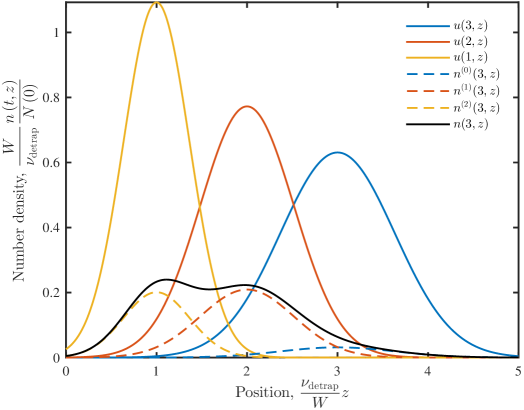
Figure 5: The solution $n\left(t,z\right)$ of the generalised diffusion equation (88) is written by sampling from the Gaussian solution $u\left(t,z\right)$ of the standard diffusion equation (105) at multiple points in time. This is done using the subordination transformation (107). Here, traps are of fixed duration, $\nu_{\mathrm{detrap}}t=1$, as described by the waiting time distribution $\phi\left(t\right)/\nu_{\mathrm{detrap}}=\delta\left(\nu_{\mathrm{detrap}}t-1\right)$. In this case, the subordination transformation becomes the summation (110) whose individual terms $n^{\left(k\right)}\left(t,z\right)$ correspond to those free particles which have been trapped $k$ times in the past. Here, there is no recombination, $\nu_{\mathrm{loss}}^{\left(\mathrm{free}\right)}=\nu_{\mathrm{loss}}^{\left(\mathrm{trap}\right)}=0$, the trapping rate is set to $\nu_{\mathrm{trap}}/\nu_{\mathrm{detrap}}=1$ and the diffusion coefficient is made small so as to emphasise each individual Gaussian’s contribution to the solution, $D\nu_{\mathrm{detrap}}/W^{2}=1/15$.

Note that, as the subordination transformation acts on time alone, the same mapping operator $\mathcal{A}$ can be used to map between spatial moments of the normal and generalised diffusion equations

$$\left\langle\mathbf{r}\right\rangle^{\left(\mathrm{GDE}\right)}\left(t\right) = \mathcal{A}\left\langle\mathbf{r}\right\rangle^{\left(\mathrm{SDE}\right)}\left(t\right),$$ (113)

$$\left\langle\mathbf{r}\mathbf{r}\right\rangle^{\left(\mathrm{GDE}\right)}\left(t\right) = \mathcal{A}\left\langle\mathbf{r}\mathbf{r}\right\rangle^{\left(\mathrm{SDE}\right)}\left(t\right),$$ (114)

where the superscript “(GDE)” denotes the generalised diffusion equation (88) and “(SDE)” denotes the standard diffusion equation (105). Additionally, the commutation relationship

$$\left[\mathcal{A},\frac{\mathrm{d}}{\mathrm{d}t}\right]\equiv\left[\nu_{\mathrm{loss}}^{\left(\mathrm{free}\right)}+\nu_{\mathrm{trap}}\left(1-\Phi\left(t\right)\ast\right)\right]\mathcal{A},$$ (115)

also allows the centre of mass (CM) transport coefficients for each diffusion equation to be related through the subordination transformation $\mathcal{A}$

$$\mathbf{W}_{\mathrm{CM}}^{\left(\mathrm{GDE}\right)}\left(t\right)=\mathrm{\mathcal{A}}\mathbf{W}_{\mathrm{CM}}^{\left(\mathrm{SDE}\right)}\left(t\right)-\left[\nu_{\mathrm{loss}}^{\left(\mathrm{free}\right)}+\nu_{\mathrm{trap}}\left(1-\Phi\left(t\right)\ast\right)\right]\mathcal{A}\left\langle\mathbf{r}\right\rangle^{\left(\mathrm{SDE}\right)}\left(t\right),$$ (116)

$$\mathbf{D}_{\mathrm{CM}}^{\left(\mathrm{GDE}\right)}\left(t\right)=\mathcal{A}\mathbf{D}_{\mathrm{CM}}^{\left(\mathrm{SDE}\right)}\left(t\right)\\ -\frac{1}{2}\left[\nu_{\mathrm{loss}}^{\left(\mathrm{free}\right)}+\nu_{\mathrm{trap}}\left(1-\Phi\left(t\right)\ast\right)\right]\mathcal{A}\left[\left\langle\mathbf{r}\mathbf{r}\right\rangle^{\left(\mathrm{SDE}\right)}\left(t\right)-\left\langle\mathbf{r}\right\rangle^{\left(\mathrm{SDE}\right)}\left(t\right)\left\langle\mathbf{r}\right\rangle^{\left(\mathrm{SDE}\right)}\left(t\right)\right],$$ (117)

where the CM transport coefficients are defined in terms of spatial moments according to Eqs. (39) and (40).

VII Conclusion

We have considered a general phase-space kinetic equation (1) which considers transport of charged particles via both delocalised and localised states, including collisional trapping, detrapping and recombination processes. The solution of this model was found analytically in Fourier-Laplace space which in turn provided analytical expressions for phase-space averaged spatial and velocity moments. These moments provided determination of both centre of mass (CM) and flux transport coefficients. As consequence of the processes of trapping and detrapping, the free particle CM transport coefficients were found to be transiently negative for high trapping rates. We have also shown that, in the hydrodynamic regime, a number of diffusion equations accurately describe the generalised Boltzmann equation (1). These include the standard diffusion equation (82), the generalised diffusion equation (88) and, when transport is dispersive, the Caputo fractional diffusion equation (101). Finally, we have written the solution of the generalised diffusion equation (88) as a subordination transformation (107) from the corresponding solution of a standard diffusion equation (105).

The model of focus in this work, Eqs. (1)-(8), was considered only for constant process rates, independent of particle energy. Extension to higher order balance equations (e.g. momentum and energy) including energy dependent rates represents the next step in extending this model. This will facilitate the generalisation of well known empirical relationships (e.g. Generalised Einstein relations, Wannier energy relation, mobility expressions) to include combined localised/delocalised transport systems. Additionally, for our model to be applied to transport in dense fluids, it is necessary to have reasonable inputs $\nu_{\mathrm{trap}}$ and $\phi\left(t\right)$. Although there are many investigations of the trapping, for example light-particle solvation in the literature (Ceperley and Alder, 1980; Miller and Reese, 2008; Cao and Berne, 1993), including free-energy changes and solvation time-scales, none of these directly produce an energy-dependent trapping frequency or waiting time distribution. The ab initio calculation of such capture collision frequencies and waiting time distributions in liquids and dense gases remains the focus of our current attention.

Appendix A List of limiting ratios of detrapping and trapping rates $R$

Table 1: Specific cases of the dimensionless quantity $R$ that is defined in Eq. (62) as the limiting ratio of particle detrapping and trapping rates. From its alternate definition (63), it can be seen that $R$ is a function of the difference in recombination loss rates $\Delta\nu_{\mathrm{loss}}\equiv\nu_{\mathrm{loss}}^{\left(\mathrm{free}\right)}-\nu_{\mathrm{loss}}^{\left(\mathrm{trap}\right)}$.

Trap type	Waiting time distribution $\phi\left(t\right)$	Limiting ratio of detrapping and trapping rates $R$
Instantaneous	$\delta\left(t\right)$	$1$
Fixed delay	$\delta\left(t-\nu_{\mathrm{detrap}}^{-1}\right)$	$\frac{\nu_{\mathrm{detrap}}}{\nu_{\mathrm{trap}}}W_{\mathrm{Lambert}}\left[\frac{\nu_{\mathrm{trap}}}{\nu_{\mathrm{detrap}}}\exp\left(\frac{\Delta\nu_{\mathrm{loss}}+\nu_{\mathrm{trap}}}{\nu_{\mathrm{detrap}}}\right)\right]\dagger$
Poisson process	$\nu_{\mathrm{detrap}}\mathrm{e}^{-\nu_{\mathrm{detrap}}t}$	$\frac{\Delta\nu_{\mathrm{loss}}+\nu_{\mathrm{trap}}-\nu_{\mathrm{detrap}}+\sqrt{\left(\Delta\nu_{\mathrm{loss}}+\nu_{\mathrm{trap}}+\nu_{\mathrm{detrap}}\right)^{2}-4\nu_{\mathrm{detrap}}\Delta\nu_{\mathrm{loss}}}}{2\nu_{\mathrm{trap}}}$
Multiple trapping model	$\alpha\nu_{0}\left(\nu_{0}t\right)^{-\alpha-1}\gamma\left(\alpha+1,\nu_{0}t\right)$	$\ddagger$

$\dagger$ The Lambert W-function is defined as satisfying

$$W_{\mathrm{Lambert}}\left(z\right)\mathrm{e}^{W_{\mathrm{Lambert}}\left(z\right)}\equiv z.$$ (118)

$\ddagger$ $R$ is the positive solution of the transcendental equation

$$R=-\frac{\alpha\pi}{\sin\alpha\pi}\left(-\frac{\Delta\nu_{\mathrm{loss}}+\nu_{\mathrm{trap}}\left(1-R\right)}{\nu_{0}}\right)^{\alpha}-\alpha\Phi_{\mathrm{Lerch}}\left(\frac{\Delta\nu_{\mathrm{loss}}+\nu_{\mathrm{trap}}\left(1-R\right)}{\nu_{0}},1,-\alpha\right),$$ (119)

where the Lerch transcendent is defined

$$\Phi_{\mathrm{Lerch}}\left(z,s,a\right)\equiv\sum_{n\geq 0}\frac{z^{n}}{\left(n+a\right)^{s}}.$$ (120)

Appendix B List of subordination transformation kernels $A\left(\tau,t\right)$

Table 2: Specific cases of the integral kernel (108), $A\left(\tau,t\right)$, used in the subordination transformation (107) that maps from the solution of the standard diffusion equation (105) to that of the generalised diffusion equation (88).

Trap type	Waiting time distribution $\phi\left(t\right)$	Scaled subordination kernel $\mathrm{e}^{\left(\nu_{\mathrm{loss}}^{\left(\mathrm{free}\right)}+\nu_{\mathrm{trap}}\right)\tau}A\left(\tau,t\right)$
Instantaneous	$\delta\left(t\right)$	$\mathrm{e}^{\nu_{\mathrm{trap}}\tau}\mathrm{e}^{-\nu_{\mathrm{loss}}^{\left(\mathrm{trap}\right)}t}\delta\left(t\right)$
Fixed delay	$\delta\left(t-\nu_{\mathrm{detrap}}^{-1}\right)$	$\mathrm{e}^{-\nu_{\mathrm{loss}}^{\left(\mathrm{trap}\right)}t}\frac{\left(\nu_{\mathrm{trap}}\tau\right)^{\nu_{\mathrm{detrap}}t}}{\Gamma\left(1+\nu_{\mathrm{detrap}}t\right)}\mathrm{III}_{\nu_{\mathrm{detrap}}^{-1}}\left(t\right)\dagger$
Poisson process	$\nu_{\mathrm{detrap}}\mathrm{e}^{-\nu_{\mathrm{detrap}}t}$	$\delta\left(t\right)+\frac{1}{t}\mathrm{e}^{-\nu_{\mathrm{detrap}}t}\sqrt{\nu_{\mathrm{trap}}\tau\nu_{\mathrm{detrap}}t}I_{1}\left(2\sqrt{\nu_{\mathrm{trap}}\tau\nu_{\mathrm{detrap}}t}\right)\ddagger$
Multiple trapping model	$\alpha\nu_{0}\left(\nu_{0}t\right)^{-\alpha-1}\gamma\left(\alpha+1,\nu_{0}t\right)$	$\mathrm{e}^{-\nu_{\mathrm{loss}}^{\left(\mathrm{trap}\right)}t}\left[\frac{1}{t_{\alpha}}l_{\alpha}\left(\frac{t}{t_{\alpha}}\right)\ast g\left(t\right)\right]\mathsection$

$\dagger$ The Dirac comb of period $T$ is defined

$$\mathrm{III}_{T}\left(t\right)\equiv\sum_{n\in\mathbb{Z}}\delta\left(t-nT\right).$$ (121)

$\ddagger$ The modified Bessel function of the first kind of order $\nu$ is defined

$$I_{\nu}\left(z\right)\equiv\sum_{n\geq 0}\frac{\left(\frac{z}{2}\right)^{2n+\nu}}{n!\Gamma\left(1+n+\nu\right)}.$$ (122)

$\mathsection$ The characteristic time $t_{\alpha}$ is defined

$$\nu_{0}t_{\alpha}\equiv\sqrt[\alpha]{\frac{\alpha\pi}{\sin\alpha\pi}\nu_{\mathrm{trap}}\tau},$$ (123)

we define in Laplace space the one-sided Lévy density

$$l_{\alpha}\left(p\right)\equiv\mathrm{e}^{-p^{\alpha}},$$ (124)

and in Laplace space

$$g\left(p\right)\equiv\exp\left[-\alpha\Phi_{\mathrm{Lerch}}\left(-\frac{p}{\nu_{0}},1,-\alpha\right)\right],$$ (125)

where the Lerch transcendent $\Phi_{\mathrm{Lerch}}\left(z,s,a\right)$ is given by Eq. (120).

References

- Metzler and Klafter (2000) R. Metzler and J. Klafter, Physics Reports 339, 1 (2000).
- Scher and Montroll (1975) H. Scher and E. W. Montroll, Physical Review B 12, 2455 (1975).
- Sibatov and Uchaikin (2007) R. T. Sibatov and V. V. Uchaikin, Semiconductors 41, 335 (2007).
- Mauracher et al. (2014) A. Mauracher, M. Daxner, J. Postler, S. E. Huber, S. Denifl, P. Scheier, and J. P. Toennies, Journal of Physical Chemistry Letters 5, 2444 (2014).
- Borghesani and Santini (2002) A. F. Borghesani and M. Santini, Physical Review E - Statistical, Nonlinear, and Soft Matter Physics 65, 056403 (2002).
- Sakai et al. (1992) Y. Sakai, W. F. Schmidt, and A. Khrapak, Chemical Physics 164, 139 (1992).
- Stepanov et al. (2012) S. V. Stepanov, V. M. Byakov, D. S. Zvezhinskiy, G. Duplâtre, R. R. Nurmukhametov, and P. S. Stepanov, Advances in Physical Chemistry 2012, 1 (2012), arXiv:1203.5390 .
- Stepanov et al. (2002) S. V. Stepanov, V. M. Byakov, B. N. Ganguly, D. Gangopadhyay, T. Mukherjee, and B. Dutta-Roy, Physica B: Condensed Matter 322, 68 (2002).
- Drachman et al. (2000) R. J. Drachman, M. Charlton, and J. W. Humberston, Advances In Atomic And Molecular Physics (Cambridge University Press, Cambrigde, 2000) p. 466.
- Colucci et al. (2011) M. G. Colucci, D. P. van der Werf, and M. Charlton, Journal of Physics B: Atomic, Molecular and Optical Physics 44, 175204 (2011).
- Barkai (2001) E. Barkai, Physical Review E 63, 46118 (2001).
- Metzler et al. (1999) R. Metzler, E. Barkai, and J. Klafter, Physical Review Letters 82, 3563 (1999).
- Robson and Blumen (2005) R. E. Robson and A. Blumen, Physical Review E 71, 061104 (2005).
- Philippa et al. (2014) B. Philippa, R. E. Robson, and R. D. White, New Journal of Physics 16, 073040 (2014).
- Bhatnagar et al. (1954) P. L. Bhatnagar, E. P. Gross, and M. Krook, Physical Review 94, 511 (1954).
- Cocks et al. (2016) D. Cocks et al., (2016), in preparation.
- Robson (1975) R. Robson, Australian Journal of Physics 28, 523 (1975).
- Fried and Conte (1961) B. D. Fried and S. D. Conte, The Plasma Dispersion Function (Academic Press, New York, 1961).
- Chapman and Cowling (1970) S. Chapman and T. G. Cowling, The Mathematical Theory of Non-uniform Gases: An Account of the Kinetic Theory of Viscosity, Thermal Conduction and Diffusion in Gases (Cambridge University Press, 1970).
- Mainardi et al. (2001) F. Mainardi, Y. Luchko, and G. Pagnini, Fractional Calculus and Applied Analysis 4, 153 (2001).
- Metzler and Klafter (2004) R. Metzler and J. Klafter, Journal of Physics A: Mathematical and General 37, R161 (2004).
- Podlubny (1998) I. Podlubny, Fractional differential equations, Vol. 198 (Academic Press, 1998).
- Ford and Simpson (2001) N. Ford and A. Simpson, Numerical Algorithms 26, 333 (2001).
- Fukunaga and Shimizu (2011) M. Fukunaga and N. Shimizu, in ASME 2011 International Design Engineering Technical Conferences and Computers and Information in Engineering Conference (American Society of Mechanical Engineers, 2011) pp. 169–178.
- Stokes et al. (2015) P. W. Stokes, B. Philippa, W. Read, and R. D. White, Journal of Computational Physics 282, 334 (2015).
- Ceperley and Alder (1980) D. M. Ceperley and B. J. Alder, Physical Review Letters 45, 566 (1980).
- Miller and Reese (2008) B. N. Miller and T. L. Reese, Physical Review E - Statistical, Nonlinear, and Soft Matter Physics 78, 061123 (2008), arXiv:0503630v1 [arXiv:cond-mat] .
- Cao and Berne (1993) J. Cao and B. J. Berne, The Journal of Chemical Physics 99, 2902 (1993).