Large-scale subspace clustering
using sketching and validation

Abstract

The nowadays massive amounts of generated and communicated data present major challenges in their processing. While capable of successfully classifying nonlinearly separable objects in various settings, subspace clustering (SC) methods incur prohibitively high computational complexity when processing large-scale data. Inspired by the random sampling and consensus (RANSAC) approach to robust regression, the present paper introduces a randomized scheme for SC, termed sketching and validation (SkeVa-)SC, tailored for large-scale data. At the heart of SkeVa-SC lies a randomized scheme for approximating the underlying probability density function of the observed data by kernel smoothing arguments. Sparsity in data representations is also exploited to reduce the computational burden of SC, while achieving high clustering accuracy. Performance analysis as well as extensive numerical tests on synthetic and real data corroborate the potential of SkeVa-SC and its competitive performance relative to state-of-the-art scalable SC approaches.
Keywords. Subspace clustering, big data, kernel smoothing, randomization, sketching, validation, sparsity.

1 Introduction

The turn of the decade has trademarked society and computing research with a “data deluge” [1]. As the number of smart and internet-capable devices increases, so does the amount of data that is generated and collected. While it is desirable to mine information from this data, their sheer amount and dimensionality introduces numerous challenges in their processing and pattern analysis, since available statistical inference and machine learning approaches do not necessarily scale well with the number of data and their dimensionality. In addition, as the cost of cloud computing is rapidly declining [2], there is a need for redesigning those traditional approaches to take advantage of the flexibility that has emerged from distributing required computations to multiple nodes, as well as reducing the per-node computational burden.

Clustering (unsupervised classification) is a method of grouping unlabeled data with widespread applications across the fields of data mining, signal processing, and machine learning. $K$-means is one of the most successful clustering algorithms due to its simplicity [3]. However, $K$-means, as well as its kernel-based variants, provides meaningful clustering results only when data, after mapped to an appropriate feature space, form “tight” groups that can be separated by hyperplanes [4].

Subspace clustering (SC) is a popular method that can group non-linearly separable data which are generated by a union of (affine) subspaces in a high-dimensional Euclidean space [5]. SC has well-documented impact in various applications, as diverse as image and video segmentation and identification of switching linear systems in controls [5]. Recent advances advocate SC algorithms with high clustering performance at the price of high computational complexity [5].

The goal of this paper is to introduce a randomized framework for reducing the computational burden of SC algorithms when the number of available data becomes prohibitively large, while maintaining high levels of clustering accuracy. The starting point is our sketching and validation (SkeVa) approach in [6]. SkeVa offers a low-computational complexity, randomized scheme for multimodal probability density function (pdf) estimation, since it draws random computationally affordable sub-populations of data to obtain a crude sketch of the underlying pdf of the massive data population. A validation step, based on divergences of pdfs, follows to assess the quality of the crude sketch. These sketching and validation phases are repeated independently for a pre-fixed number of times, and the draw achieving the “best score” is finally utilized to cluster the whole data population. SkeVa is inspired from the random sampling and consensus (RANSAC) method [7]. Although RANSAC’s principal field of application is the parametric regression problem in the presence of outliers, it has been also employed in SC [5].

To achieve the goal of devising an SC scheme with low computational complexity footprint, the present paper broadens the scope of SkeVa to the SC context. Moreover, to support the state-of-the-art performance of SkeVa on real-data, this contribution provides a rigorous performance analysis on the lower bound of the number of independent draws for SkeVa to identify a draw that “represents well” the underlying data pdf, with high probability. The analysis is facilitated by the non-parametric estimation framework of kernel smoothing [8], and models the underlying data pdf as a mixture of Gaussians, which are known to offer universal pdf approximations [9, 10]. To assess the proposed SkeVa-SC, extensive numerical tests on synthetic and real-data are presented to underline the competitive performance of SkeVa-SC relative to state-of-the-art scalable SC approaches.

The rest of the paper is organized as follows. Section 2 provides SC preliminaries along with notation and tools for kernel density estimation. Section 3 introduces the proposed algorithm for large-scale SC, while Section 4 provides performance bounds for SkeVa-SC. Section 5 presents numerical tests conducted to evaluate the performance of SkeVa-SC in comparison with state-of-the-art SC algorithms. Finally, concluding remarks and future research directions are given in Section 6.

Notation: Unless otherwise noted, lowercase bold letters, $\bm{x}$, denote vectors, uppercase bold letters, $\mathbf{X}$, represent matrices, and calligraphic uppercase letters, $\mathcal{X}$, stand for sets. The $(i,j)$th entry of matrix $\mathbf{X}$ is denoted by $[\mathbf{X}]_{ij}$; $\mathbb{R}^{D}$ stands for the $D$-dimensional real Euclidean space, $\mathbb{R}_{+}$ for the set of positive real numbers, $\operatorname{\mathbb{E}}[\cdot]$ for expectation, and $\|\cdot\|$ for the $L_{2}$-norm.

2 Preliminaries

2.1 SC problem statement

Consider data $\{\bm{x}_{i}\in\mathbb{R}^{D}\}_{i=1}^{N}$ drawn from a union of $K$ affine subspaces, each denoted by $\mathcal{S}_{k}$, adhering to the model:

$$\bm{x}_{i}=\mathbf{U}_{k}\bm{y}_{i}+\bm{m}_{k}+\bm{v}_{i}\,,\quad\forall\bm{x}_{i}\in\mathcal{S}_{k}$$ (1)

where $d_{k}$ (possibly with $d_{k}\ll D$) is the dimensionality of $\mathcal{S}_{k}$; $\mathbf{U}_{k}$ is a $D\times d_{k}$ matrix whose columns form a basis of $\mathcal{S}_{k}$, $\bm{y}_{i}\in\mathbb{R}^{d_{k}}$ is the low-dimensional representation of $\bm{x}_{i}$ in $\mathcal{S}_{k}$ with respect to (w.r.t.) $\mathbf{U}_{k}$, $\bm{m}_{k}\in\mathbb{R}^{D}$ is the “centroid” or intercept of $\mathcal{S}_{k}$, and $\bm{v}_{i}\in\mathbb{R}^{D}$ denotes the noise vector capturing unmodeled effects. If $\mathcal{S}_{k}$ is linear then $\bm{m}_{k}=\bm{0}$. Using (1), any $\bm{x}_{i}$ can be described as

$$\bm{x}_{i}=\sum_{k=1}^{K}[\bm{\pi}_{i}]_{k}\left(\mathbf{U}_{k}\bm{y}_{i}+\bm{m}_{k}\right)+\bm{v}_{i}$$ (2)

where $\bm{\pi}_{i}$ is the cluster assignment vector for $\bm{x}_{i}$ and $[\bm{\pi}_{i}]_{k}$ denotes the $k$th entry of $\bm{\pi}_{i}$ under the constraints of $[\bm{\pi}_{i}]_{k}\geq 0$ and $\sum_{k=1}^{K}[\bm{\pi}_{i}]_{k}=1$. If $\bm{\pi}_{i}\in\{0,1\}^{K}$ then datum $\bm{x}_{i}$ lies in only one subspace (hard clustering), while if $\bm{\pi}_{i}\in[0,1]^{K}$, then $\bm{x}_{i}$ can belong to multiple clusters (soft clustering). In the latter case, $[\bm{\pi}_{i}]_{k}$ can be thought of as the probability that datum $\bm{x}_{i}$ belongs to $\mathcal{S}_{k}$.

Given the data matrix $\mathbf{X}:=[\bm{x}_{1},\bm{x}_{2},\ldots,\bm{x}_{N}]\in\mathbb{R}^{D\times N}$ and the number of subspaces $K$, SC involves finding the data-to-subspace assignment vectors $\{\bm{\pi}_{i}\}_{i=1}^{N}$, the subspace bases $\left\{\mathbf{U}_{k}\right\}_{k=1}^{K}$, their dimensions $\{d_{k}\}_{k=1}^{K}$, the low-dimensional representations $\{\bm{y}_{i}\}_{i=1}^{N}$, as well as the centroids $\{\bm{m}_{k}\}_{k=1}^{K}$ [5]. SC can be formulated as follows

$$\underset{\mathbf{\Pi},\{\mathbf{U}_{k}\},\{\bm{y}_{i}\},\mathbf{M}}{\min} \sum_{k=1}^{K}\sum_{i=1}^{N}[\bm{\pi}_{i}]_{k}\|\bm{x}_{i}-\mathbf{U}_{k}\bm{y}_{i}-\bm{m}_{k}\|_{2}^{2}$$ (3)

subject to (s.to) $$\mathbf{\Pi}^{\top}\bm{1}=\bm{1};\quad[\bm{\pi}_{i}]_{k}\geq 0,\ \forall(i,k)$$

where $\mathbf{\Pi}:=[\bm{\pi}_{1},\ldots,\bm{\pi}_{N}]$, $\mathbf{M}:=[\bm{m}_{1},\bm{m}_{2},\ldots,\bm{m}_{K}]$, and $\bm{1}$ denotes the all-ones vector of matching dimensions.

The problem in (3) is non-convex as all of $\mathbf{\Pi},\{\mathbf{U}_{k}\}_{k=1}^{K},\{d_{k}\}_{k=1}^{K},\{\bm{y}_{i}\}_{i=1}^{N}$, and $\mathbf{M}$ are unknown. We outline next a popular alternating way of solving (3). For given $\bm{\Pi}$ and $\{d_{k}\}_{k=1}^{K}$, bases of the subspaces can be recovered using the singular value decomposition (SVD) on the data associated with each subspace. Indeed, given $\mathbf{X}_{k}:=[\bm{x}_{i_{1}},\ldots,\bm{x}_{i_{N_{k}}}]$, associated with $\mathcal{S}_{k}$ ($\sum_{k=1}^{K}N_{k}=N$), a basis $\mathbf{U}_{k}$ can be obtained from the first $d_{k}$ (from the left) singular vectors of $\mathbf{X}_{k}-[\bm{m}_{k},\ldots,\bm{m}_{k}]$ where $\bm{m}_{k}=(1/N_{k})\sum_{i\in\mathcal{S}_{k}}\bm{x}_{i}$. On the other hand, when $\{\mathbf{U}_{k},\bm{m}_{k}\}_{k=1}^{K}$ are given, the assignment matrix $\bm{\Pi}$ can be recovered in the case of hard clustering by finding the closest subspace to each datapoint; that is, $\forall i\in\{1,2,\ldots,N\}$, $\forall k\in\{1,\ldots,K\}$, we obtain

$$[\bm{\pi}_{i}]_{k}=\begin{cases}1,&\text{if}\ k=\operatorname*{arg\;min}\limits_{k^{\prime}\in\{1,\ldots,K\}}\left\|\bm{x}_{i}-\bm{m}_{k^{\prime}}-\mathbf{U}_{k^{\prime}}\mathbf{U}_{k^{\prime}}^{\top}\bm{x}_{i}\right\|_{2}^{2}\\ 0,&\text{otherwise}\end{cases}$$ (4)

where $\|\bm{x}_{i}-\bm{m}_{k}-\mathbf{U}_{k}\mathbf{U}_{k}^{\top}\bm{x}_{i}\|_{2}$ is the distance of $\bm{x}_{i}$ from $\mathcal{S}_{k}$.

The $K$-subspaces algorithm [11], which is a generalization of the ubiquitous $K$-means one [12] for SC, builds upon this alternating minimization of (3): (i) First, fixing $\mathbf{\Pi}$ and then solving for the remaining unknowns; and (ii) fixing $\{\mathbf{U}_{k},\bm{m}_{k}\}_{k=1}^{K}$, and then solving for $\mathbf{\Pi}$. Since SVD is involved, SC entails high computational complexity, whenever $d_{k}$ and/or $N_{k}$ are massive. Specifically the SVD of a $D\times N_{k}$ matrix incurs a computational complexity of $\mathcal{O}(\alpha D^{2}N_{k}+\beta N_{k}^{3})$, where $\alpha,\beta$ are algorithm-dependent constants.

It is known that when $K=1$ and $\mathbf{U}$ is orthonormal, (3) boils down to PCA [13]

$$\underset{\mathbf{U},\{\bm{y}_{i}\},\mathbf{M}}{\min} \sum_{i=1}^{N}\|\bm{x}_{i}-\mathbf{U}\bm{y}_{i}-\bm{m}\|_{2}^{2}$$ (5)

s.to $$\mathbf{U}^{\top}\mathbf{U}=\mathbf{I}_{d}$$

where $\mathbf{I}_{d}$ ($d:=d_{k}$) stands for the $d\times d$ identity matrix. Notice that for $K=1$, it holds that $[\bm{\pi}_{i}]_{k}=1$. Moreover, if $\mathbf{U}_{k}:=\bm{0}$, $\forall k$, with $K>1$ looking for $\{\bm{m}_{k},\bm{\pi}_{k}\}_{k=1}^{K}$ amounts to ordinary clustering

$$\underset{\mathbf{\Pi},\mathbf{M}}{\min} \sum_{k=1}^{K}\sum_{i=1}^{N}[\bm{\pi}_{i}]_{k}\|\bm{x}_{i}-\bm{m}_{k}\|_{2}^{2}$$ (6)

s.to $$\mathbf{\Pi}^{\top}\bm{1}=\bm{1}\,.$$

Finally, it is also well known that (6) with $\bm{\pi}\in[0,1]^{K}$ (soft clustering) amounts to pdf estimation [3]. This fact will be exploited by our novel approach to perform on large-scale SC, and link the benefits of pdf estimation with those of high-performance SC algorithms.

2.2 Kernel density estimation

Kernel smoothing or kernel density estimation [8] is a non-parametric approach to estimating pdfs. Kernel density estimators, similar to the histogram and unlike parametric estimators, make minimal assumptions about the unknown pdf, $f$. Because they employ general kernel functions rather than rectangular bins, kernel smoothers are flexible to attain faster convergence rates than the histogram estimator as the number of observed data, $n$, tends to infinity [8]. However, their convergence rate is slower than that of parametric estimators. For data $\{\bm{x}_{i}\}_{i=1}^{n}\sim f$, drawn from $f$, the kernel density estimator of $f$ is given by [8]

$$\hat{f}(\bm{x})=\frac{1}{n}\sum_{i=1}^{n}K_{\mathbf{H}}(\bm{x}-\bm{x}_{i})\$$ (7)

where $K_{\mathbf{H}}(\bm{x}-\bm{x}_{i})$ denotes a pre-defined kernel function centered at $\bm{x}_{i}$, with a positive-definite bandwidth matrix $\mathbf{H}\in\mathbb{R}^{D\times D}$. This bandwidth matrix controls the amount of smoothing across dimensions. Typically, $K_{\mathbf{H}}(\bm{x})$ is chosen to be a density so that $\hat{f}(\bm{x})$ is also a pdf. The role of bandwidth can be understood clearly as $\mathbf{H}$ corresponds to the covariance matrix of the pdf $K_{\mathbf{H}}(\bm{x})$ [8].

The performance of kernel-based estimators is usually assessed using the mean-integrated square error (MISE)

$$\text{MISE}(\hat{f};\mathbf{H}):=\operatorname{\mathbb{E}}\left[\int\left(f(\bm{x})-\hat{f}(\bm{x})\right)^{2}d\bm{x}\right]$$ (8)

where $\int$ denotes $D$-dimensional integration, and $d\bm{x}$ stands for $dx_{1}\ldots dx_{D}$, with $\bm{x}:=[x_{1},\ldots,x_{D}]^{\top}$. The choice of $\mathbf{H}$ has a notable effect on MISE. As a result, it makes sense to select $\mathbf{H}$ such that the MISE is low.

Letting $\mathbf{H}:=h^{2}\mathbf{I}_{D}$ with $h>0$, facilitates the minimization of (8) w.r.t. $h$, especially if $h$ is regarded as a function of $n$, i.e., $h:=h(n)$, and satisfies

$$\lim_{n\rightarrow\infty}h=0,\quad\lim_{n\rightarrow\infty}nh=\infty\,.$$ (9)

Using the $D$-variate Taylor expansion of $f$ the asymptotically MISE optimal $h$ is [8]:

$$h^{*}=\left[\frac{D\int K^{2}(\bm{x})d\bm{x}}{n\int{x_{i}^{2}}K(\bm{x})d\bm{x}\int(\nabla^{2}f(\bm{x}))^{2}d\bm{x}}\right]^{1/(D+4)}$$ (10)

where $\int x_{i}^{2}K(\bm{x})d\bm{x}$ is not a function of $i$, when $K(\bm{x})$ is a spherically symmetric compactly supported density, and $\nabla^{2}f(\bm{x}):=\sum_{i=1}^{D}\frac{\partial^{2}f(\bm{x})}{\partial x_{i}^{2}}$. In addition, when the density $f$ to be estimated is a mixture of Gaussians [9, 10], and the kernel is chosen to be a Gaussian density $K_{\mathbf{H}}(\bm{x}-\bm{x}_{i}):=\phi_{\mathbf{H}}(\bm{x}-\bm{x}_{i})$, where

$$\phi_{\mathbf{H}}(\bm{x}-\bm{x}_{i}):=\frac{1}{(2\pi)^{D/2}|\mathbf{H}|^{1/2}}\exp\left(-\frac{1}{2}(\bm{x}-\bm{x}_{i})^{\top}\mathbf{H}^{-1}(\bm{x}-\bm{x}_{i})\right)$$ (11)

with mean $\bm{x}_{i}$ and covariance matrix $\mathbf{H}$, it is possible to express (8) in closed form. This closed-form is due to the fact that convolution of Gaussians is also Gaussian; that is,

$$\int\phi_{\mathbf{H}_{i}}(\bm{x}-\bm{x}_{i})\phi_{\mathbf{H}_{j}}(\bm{x}-\bm{x}_{j})d\bm{x}=\phi_{(\mathbf{H}_{i}+\mathbf{H}_{j})}(\bm{x}_{i}-\bm{x}_{j})\,.$$ (12)

If $K_{\mathbf{H}}(\bm{x})=\phi_{\mathbf{I}_{D}}(\bm{x})$, the optimal bandwidth of (10) becomes

$$h^{*}=\left[\frac{D\phi_{2\mathbf{I}_{D}}(\bm{0})}{n\int(\nabla^{2}f(\bm{x}))^{2}d\bm{x}}\right]^{1/(D+4)}\,.$$ (13)

The proposed SC algorithm of Section 3 will draw ideas from kernel density estimation, and a proper choice of $h$ will be proved to be instrumental in optimizing SC performance.

2.3 Prior work

Besides the $K$-subspaces solver outlined in Sec. 2.1, various algorithms have been developed by the machine learning [5] and data-mining community [14] to solve (3). A probabilistic (soft) counterpart of $K$-subspaces is the mixture of probabilistic PCA [15], which assumes that data are drawn from a mixture of degenerate (having zero variance in some dimensions) Gaussians. Building on the same assumption, the agglomerative lossy compression (ALC) [16] utilizes ideas from rate-distortion theory [17] to minimize the required number of bits to “encode” each cluster, up to a certain distortion level. Algebraic schemes, such as the Costeira-Kanade algorithm [18] and Generalized PCA (GPCA [19]), aim to tackle SC from a linear algebra point of view, but generally their performance is guaranteed only for independent and noise-less subspaces. Other methods recover subspaces by finding local linear subspace approximations [20]. See also [21, 22] for online clustering approaches to handling streaming data.

Arguably the most successful class of solvers for (3) relies on spectral clustering [23] to find the data-to-subspace assignments. Algorithms in this class generate first an $N\times N$ affinity matrix $\mathbf{A}$ to capture the similarity between data, and then perform spectral clustering on $\mathbf{A}$. Matrix $\mathbf{A}$ implies a graph $\mathcal{G}$ whose vertices correspond to data and edge weights between data are given by its entries. Spectral clustering algorithms form the graph Laplacian matrix

$$\mathbf{L}:=\mathbf{D}-\mathbf{A}$$ (14)

where $\mathbf{D}$ is a diagonal matrix such that (s.t.) $[\mathbf{D}]_{ii}=\sum_{j=1}^{N}[\mathbf{A}]_{ij}$. The algebraic multiplicity of the $0$ eigenvalue of $\mathbf{L}$ yields the number of connected components in $\mathcal{G}$ [23], while the corresponding eigenvectors are indicator vectors of the connected components. For the sake of completeness, Alg. 1 summarizes the procedure of how the trailing eigenvectors of $\mathbf{L}$ are used to obtain cluster assignments in spectral clustering.

1:Data affinity matrix $\mathbf{A}$; number of clusters $K$.

2:Data-cluster associations.

3: Form diagonal matrix $\mathbf{D}$, with entries $[\mathbf{D}]_{ii}:=\sum_{j=1}^{N}[\mathbf{A}]_{ij}$.

4: Laplacian matrix: $\mathbf{L}:=\mathbf{D}-\mathbf{A}$.

5: Extract $K$ trailing eigenvectors $\{\mathbf{v}_{k}\in\mathbb{R}^{N}\}_{k=1}^{K}$ of $\mathbf{L}$. Let $\mathbf{V}=[\mathbf{v}_{1},\ldots,\mathbf{v}_{K}]\in\mathbb{R}^{N\times K}$.

6: Let $\{\mathbf{z}_{i}\}_{i=1}^{N}$ be the rows of $\mathbf{V}$; $\mathbf{z}_{i}$ corresponds to the $i$th vertex ($i$th datapoint).

7: Group $\{\mathbf{z}_{i}\}_{i=1}^{N}$ into $k$ clusters using $K$-means.

Algorithm 1 Unnormalized spectral clustering [23]

Sparse subspace clustering (SSC) [24] exploits the fact that under the union of subspaces model, (3), only a small percentage of data suffice to provide a low-dimensional affine representation of any $\bm{x}_{i}$, i.e., $\bm{x}_{i}=\sum_{j=1,j\neq i}^{N}w_{ij}\bm{x}_{j}$, $\forall i\in\{1,2,\ldots,N\}$. Specifically, SSC solves the following sparsity-imposing optimization problem

$$\underset{\mathbf{W}}{\min} \|\mathbf{W}\|_{1}+\lambda\|\mathbf{X}-\mathbf{X}\mathbf{W}\|_{2}^{2}$$ (15)

s.to $$\mathbf{W}^{\top}\bm{1}=\bm{1};\quad\text{diag}(\mathbf{W})=\bm{0}$$

where $\mathbf{W}:=[\bm{w}_{1},\bm{w}_{2},\ldots,\bm{w}_{N}]$; column $\bm{w}_{i}$ is sparse and contains the coefficients for the representation of $\bm{x}_{i}$; $\lambda>0$ is the regularization coefficient; and $\|\mathbf{W}\|_{1}:=\sum_{i,j=1}^{N}[\mathbf{W}]_{i,j}$. Matrix $\mathbf{W}$ is used to create the affinity matrix $[\mathbf{A}]_{ij}:=|[\mathbf{W}]_{ij}|+|[\mathbf{W}]_{ji}|$. Finally, spectral clustering, e.g., Alg. 1, is performed on $\mathbf{A}$ and cluster assignments are identified. Using those assignments, $\mathbf{M}$ is found by taking sample means per cluster, and $\{\mathbf{U}_{k}\}_{k=1}^{K}$, $\{\bm{y}_{i}\}_{i=1}^{N}$ are obtained by applying SVD on $\mathbf{X}_{k}-[\bm{m}_{k},\ldots,\bm{m}_{k}]$. For future use, SSC is summarized in Alg. 2.

The low-rank representation algorithm (LRR) [25] is similar to SSC, but replaces the $\ell_{1}$-norm in (15) with the nuclear one: $\|\mathbf{W}\|_{*}:=\sum_{i=1}^{\rho}\sigma_{i}(\mathbf{W})$, where $\rho$ stands for the rank and $\sigma_{i}(\mathbf{W})$ for the $i$th singular value of $\mathbf{W}$. The high clustering accuracy achieved by both SSC and LRR comes at the price of high complexity. Solving (15) scales quadratically with the number of data $N$, on top of performing spectral clustering across $K$ clusters, which renders SSC computationally prohibitive for large-scale SC. When data are high-dimensional ($D\gg$), methods based on (statistical) leverage scores, random projections [26], or our recent sketching and validation (SkeVa) [6] approach can be employed to reduce complexity to an affordable level. When the number of data is large ($N\gg$), the current state-of-the-art approach, scalable sparse subspace clustering (SSSC) [27], involves drawing randomly $n<N$ data, performing SSC on them, and expressing the rest of the data according to the clusters identified by that random draw of samples. While SSSC clearly reduces complexity, performance can potentially suffer as the random sample may not be representative of the entire dataset, especially when $n\ll N$ and clusters are unequally populated. To alleviate this issue, the present paper introduces a structured trial-and-error approach to identify a “representative” $n$-point sample from a dataset with $n\ll N$, while maintaining low computational complexity.

1:Data $\mathbf{X}$; number of clusters $K$; $\lambda$

2:Data-cluster associations $\mathbf{\Pi}$.

3: Solve (15) for $\mathbf{W}$.

4: $[\mathbf{A}]_{ij}:=|[\mathbf{W}]_{ij}|+|[\mathbf{W}]_{ji}|$.

5: Perform spectral clustering, namely, Alg. 1, on $\mathbf{A}$.

6: Identify point-to-subspace associations.

Algorithm 2 Sparse Subspace Clustering (SSC) [24]

Regarding kernel smoothing, most of the available algorithms address the important issue of bandwidth selection $\mathbf{H}$ to achieve desirable convergence rate properties in the approximation of the unknown pdf [28, 29, 30, 31]. The present paper, however, pioneers a framework to randomly choose the subset of kernel functions yielding a small error when estimating a multi-modal pdf.

3 The SkeVa-SC algorithm

The proposed algorithm, named SkeVa-SC, is listed in Alg. 3. It aims at iteratively finding a representative subset of $n$ randomly drawn data, $\check{\mathbf{X}}\in\mathbb{R}^{D\times n}$, run subspace clustering on $\check{\mathbf{X}}$, and associate the remaining data $\tilde{\mathbf{X}}:=\mathbf{X}\setminus\check{\mathbf{X}}\in\mathbb{R}^{D\times(N-n)}$ with the subspaces extracted from $\check{\mathbf{X}}$. SkeVa-SC draws a prescribed number of $R_{\max}$ realizations, over which two phases are performed: A sketching and a validation phase. The structure and philosophy of SkeVa-SC is based on the notion of divergences between pdfs.

Per realization $r$, the sketching stage proceeds as follows: A sub-population, $\check{\mathbf{X}}^{(r)}$, of the data is randomly drawn, and a pdf $\hat{f}^{(r)}(\bm{x})$, is estimated based on this sample using kernel smoothing. As the clusters are assumed to be sufficiently separated, $\hat{f}^{(r)}(\bm{x})$ is expected to be multimodal. To confirm this, $\hat{f}^{(r)}(\bm{x})$ is compared with a unimodal pdf $\hat{f}_{0}^{(r)}(\bm{x})$, using a measure $d(\hat{f}^{(r)},\hat{f}_{0}^{(r)})$ of pdf discrepancy. If $\hat{f}^{(r)}$ is sufficiently different from $\hat{f}_{0}^{(r)}$ then $d(\hat{f}^{(r)},\hat{f}_{0}^{(r)})\geq\Delta_{0}$, where $\Delta_{0}$ is some pre-selected threshold, SkeVa-SC proceeds to the validation stage; otherwise, SkeVa-SC deems this draw uninformative and advances to the next realization $r+1$, without performing the validation step.

At the validation stage of SkeVa-SC, another random sample of $n^{\prime}$ data, $(n\leq n^{\prime}\ll N)$, different from the one in $\check{\mathbf{X}}^{(r)}$, is drawn, forming $\tilde{\mathbf{X}}^{(r)}\in\mathbb{R}^{D\times n^{\prime}}$. The purpose of this stage is to evaluate how well $\check{\mathbf{X}}^{(r)}$ represents the whole dataset. The pdf $\tilde{f}^{(r)}(\bm{x})$ of $\tilde{\mathbf{X}}^{(r)}$ is estimated and compared to $\hat{f}^{(r)}(\bm{x})$ using $d(\hat{f}^{(r)},\tilde{f}^{(r)})$. A score $\psi[d(\hat{f}^{(r)},\tilde{f}^{(r)})]$ is assigned to $\check{\mathbf{X}}^{(r)}$, using a non-increasing scoring function $\psi:\mathbb{R}\rightarrow\mathbb{R}$ that grows as realizations $\hat{f}^{(r)}$ and $\tilde{f}^{(r)}$ come closer.

Finally, after $R_{\max}$ realizations, the set of $n$ data $\check{\mathbf{X}}^{(r^{*})}$ that received the highest score $r^{*}:=\arg\max_{r}\psi[d(\hat{f}^{(r)},\tilde{f}^{(r)})]$, is selected and SC (SSC or any other algorithm) is performed on it; that is,

$$\underset{\mathbf{W}}{\min} \|\mathbf{W}\|_{1}+\lambda\left\|\check{\mathbf{X}}^{(r^{*})}-\check{\mathbf{X}}^{(r^{*})}\mathbf{W}\right\|_{2}^{2}$$ (16)

s.to $$\mathbf{W}^{\top}\bm{1}=\bm{1};\quad\text{diag}(\mathbf{W})=\bm{0}\,.$$

The remaining data $\tilde{\mathbf{X}}^{(r^{*})}:=\mathbf{X}\setminus\check{\mathbf{X}}^{(r^{*})}$ are associated with the clusters defined by $\check{\mathbf{X}}^{(r^{*})}$. This association can be performed either by using the residual minimization method, described in SSSC [27], or, if subspace dimensions are known, by identifying the subspace that is closest to each datum, as in (4).

Remark 1.

Threshold $\Delta_{0}$ can be updated across iterations. If $\Delta_{0}^{(0)}=-\infty$ stands for the initial threshold value, $\psi_{\max}^{(r)}$ for the current maximum score as of iteration $r$ and $\psi_{\max}^{(0)}=-\infty$, the threshold, at iteration $r\in\{1,\ldots,R_{\max}\}$, is updated as

$$\Delta_{0}^{(r)}:=\begin{dcases}d(\hat{f}^{(r)},\hat{f}_{0}^{(r)})\,,&\text{ if }d(\hat{f}^{(r)},\hat{f}_{0}^{(r)})\geq\Delta_{0}^{(r-1)}\\ &\text{ and }\psi[d(\hat{f}^{(r)},\tilde{f}^{(r)})]\geq\psi_{\max}^{(r)}\\ \Delta_{0}^{(r-1)}\,,&\text{ otherwise}\,.\end{dcases}$$ (17)

Remark 2.

As SkeVa-SC realizations are drawn independently, they can be readily parallelized using schemes such as MapReduce [32].

Remark 3.

The sketching and validation scheme does not target the SC goal explicitly. Rather, it decides whether a sampled subset of data is informative or not.

To estimate the densities involved at each step of SkeVa-SC, kernel density estimators, or kernel smoothers [cf. Section 2.2] are employed. Specifically, SkeVa-SC, seeks to solve the following optimization problem: $\min_{\check{\mathbf{X}}^{(r)}}d(f,\hat{f}^{(r)})$, where $\hat{f}^{(r)}(\bm{x}):=(1/n)\sum_{i=1}^{n}K_{\mathbf{H}}(\bm{x}-\bm{x}_{i}^{(r)})$, and $\bm{x}_{i}^{(r)}$ denotes the $i$th column of $\check{\mathbf{X}}^{(r)}$. As the pdf $f$ to be estimated is generally unknown, a prudent choice for the bandwidth matrix is $\mathbf{H}:=h^{2}\mathbf{I}_{D}$ with $h>0$, as it provides isotropic smoothing across all dimensions and greatly simplifies the analysis.

To assess performance in closed form, start with the integrated square error (ISE)

$$d_{\text{ISE}}(f,g):=\int\left(f(\bm{x})-g(\bm{x})\right)^{2}d\bm{x}$$ (18)

or, as in [6], the Cauchy-Schwarz divergence [33]

$$d_{\text{CS}}(f,g):=-\log\frac{\left(\int f(\bm{x})g(\bm{x})d\bm{x}\right)^{2}}{\int f^{2}(\bm{x})d\bm{x}\int g^{2}(\bm{x})d\bm{x}}$$ (19)

which will henceforth be adopted as our dissimilarity metric $d$. Moreover, we will choose the Gaussian multivariate kernel, that is $K_{\mathbf{H}}(\bm{x}-\bm{x}_{i})=\phi_{\mathbf{H}}(\bm{x}-\bm{x}_{i})$, with $\phi_{\mathbf{H}}$ defined as (11).

1:Data $\mathbf{X}$; max. no. of iterations $R_{\max}$; bandwidth $h$

2:Clustered data; bases of subspaces

3:for $r=1$ to $R_{\max}$ do

4:    Sample $n\ll N$ columns of $\mathbf{X}$ to form $\check{\mathbf{X}}^{(r)}$.

5:    Estimate pdf $\hat{f}^{(r)}$ of $\check{\mathbf{X}}^{(r)}$; evaluate dissimilarity $d(\hat{f}^{(r)},\hat{f}_{0}^{(r)})$ from a unimodal pdf $\hat{f}_{0}^{(r)}$ [cf. (20)].

6:   if  $d(\hat{f}^{(r)},\hat{f}_{0}^{(r)})\geq\Delta_{0}$ then

7:       Sample $n^{\prime}$ $(n\leq n^{\prime}\ll N)$ new columns to form $\tilde{\mathbf{X}}^{(r)}$; evaluate pdf $\tilde{f}^{(r)}$ of $\tilde{\mathbf{X}}^{(r)}$.

8:       Find $d(\hat{f}^{(r)},\tilde{f}^{(r)})$ and score $\psi[d(\hat{f}^{(r)},\tilde{f}^{(r)})]$.

9:   end if

10:end for

11:Select winner as $r^{*}:=\arg\max_{r}\psi[d(\hat{f}^{(r)},\tilde{f}^{(r)})]$.

12:Perform SSC (Alg. 2) on $\check{\mathbf{X}}^{(r^{*})}$ to find $\mathbf{\Pi}$.

13:Associate $\mathbf{X}\setminus\check{\bm{X}}^{(r^{*})}$ to clusters defined in step 12.

Algorithm 3 Sketching and validation SC (SkeVa-SC)

The estimated pdfs that are used by SkeVa-SC are listed as follows:

$$\hat{f}^{(r)}(\bm{x}):=\frac{1}{n}\sum_{i=1}^{n}\phi_{\mathbf{H}}\left(\bm{x}-\bm{x}_{i}^{(r)}\right)$$ (20a)

$$\hat{f}_{0}^{(r)}(\bm{x}):=\phi_{\mathbf{H}_{0}}\left(\bm{x}-\frac{1}{n}\sum_{i=1}^{n}\bm{x}_{i}^{(r)}\right)$$ (20b)

$$\tilde{f}^{(r)}(\bm{x})=\frac{1}{n^{\prime}}\sum_{i=1}^{n^{\prime}}\phi_{\mathbf{H}^{\prime}}\left(\bm{x}-\tilde{\bm{x}}_{i}^{(r)}\right)$$ (20c)

where $\tilde{\bm{x}}_{i}^{(r)}$ is the $i$th column of $\tilde{\mathbf{X}}^{(r)}$, and $\mathbf{H},\mathbf{H}_{0},\mathbf{H}^{\prime}$ are appropriately defined bandwidth matrices. It is then easy to show that for a measure such as (18) or (19) several of the pdf dissimilarities can be found in closed-form as [cf. (12)]

$$d_{\text{ISE}}(\hat{f}^{(r)},\hat{f}_{0}^{(r)})= \frac{1}{n^{2}}\sum_{i=1}^{n}\sum_{j=1}^{n}\phi_{2\mathbf{H}}(\bm{x}_{i}^{(r)}-\bm{x}_{j}^{(r)})+\phi_{2\mathbf{H}_{0}}(\bm{0})-\frac{2}{n}\sum_{i=1}^{n}\phi_{\mathbf{H}+\mathbf{H}_{0}}\left(\bm{x}_{i}^{(r)}-\frac{1}{n}\sum_{i=1}^{n}\bm{x}_{i}^{(r)}\right)$$ (21a)

$$d_{\text{ISE}}(\hat{f}^{(r)},\tilde{f}^{(r)})= \frac{1}{n^{2}}\sum_{i=1}^{n}\sum_{j=1}^{n}\phi_{2\mathbf{H}}(\bm{x}_{i}^{(r)}-\bm{x}_{j}^{(r)})+\frac{1}{n^{\prime 2}}\sum_{i=1}^{n^{\prime}}\sum_{j=1}^{n^{\prime}}\phi_{2\mathbf{H}^{\prime}}(\tilde{\bm{x}}_{i}^{(r)}-\tilde{\bm{x}}_{j}^{(r)})$$

$$-\frac{2}{nn^{\prime}}\sum_{i=1}^{n}\sum_{j=1}^{n^{\prime}}\phi_{\mathbf{H}+\mathbf{H}^{\prime}}(\bm{x}_{i}^{(r)}-\tilde{\bm{x}}_{j}^{(r)})$$ (21b)

$$d_{\text{CS}}(\hat{f}^{(r)},\hat{f}_{0}^{(r)})= -2\log\left[\frac{1}{n}\sum_{i=1}^{n}\phi_{\mathbf{H}+\mathbf{H}_{0}}\left(\bm{x}_{i}^{(r)}-\frac{1}{n}\sum_{j=1}^{n}\bm{x}_{i}^{(r)}\right)\right]+\log\frac{1}{n^{2}}\sum_{i=1}^{n}\sum_{j=1}^{n}\phi_{2\mathbf{H}}\left(\bm{x}_{i}^{(r)}-\bm{x}_{j}^{(r)}\right)$$

$$+\log\phi_{2\mathbf{H}_{0}}(\bm{0})$$ (21c)

$$d_{\text{CS}}(\hat{f}^{(r)},\tilde{f}^{(r)})= -2\log\left[\frac{1}{nn^{\prime}}\sum_{i=1}^{n}\sum_{j=1}^{n^{\prime}}\phi_{\mathbf{H}+\mathbf{H}^{\prime}}\left(\bm{x}_{i}^{(r)}-\tilde{\bm{x}}_{j}^{(r)}\right)\right]+\log\frac{1}{n^{2}}\sum_{i=1}^{n}\sum_{j=1}^{n}\phi_{2\mathbf{H}}\left(\bm{x}_{i}^{(r)}-\bm{x}_{j}^{(r)}\right)$$

$$+\log\frac{1}{n^{\prime 2}}\sum_{i=1}^{n^{\prime}}\sum_{j=1}^{n^{\prime}}\phi_{2\mathbf{H}^{\prime}}\left(\tilde{\bm{x}}_{i}^{(r)}-\tilde{\bm{x}}_{j}^{(r)}\right)\,.$$ (21d)

Since finding the Gaussian dissimilarities between $n$ $D$-dimensional data incurs complexity $\mathcal{O}(Dn^{2})$, the complexity of Alg. 3 is $o[DR_{\max}(n^{2}+nn^{\prime}+n^{\prime 2})]$ per iteration, if the Gaussian kernel is utilized. As with any algorithm that involves kernel smoothing, the choice of bandwidth matrices $\mathbf{H},\mathbf{H}^{\prime},\mathbf{H}_{0}$ affects critically the performance of Alg. 3.

4 Performance Analysis

The crux of Alg. 3 is the $R_{\max}$ number of independent random draws to identify a subset of data that “represents well” the whole data population. Since SkeVa-SC aims at large-scale clustering, it is natural to ask whether $R_{\max}$ iterations suffice to mine a subset of data whose pdf approximates well the unknown $f$. It is therefore crucial, prior to any implementation of SkeVa-SC, to have an estimate of the minimum number of $R_{\max}$ that ensures an “informative draw” with high probability. Such concerns are not taken into account in SSSC [27], where only a single draw is performed prior to applying SC. This section provides analysis to establish such a lower-bound on $R_{\max}$, when the underlying pdf $f$ obeys a Gaussian mixture model (GMM). Due to the universal approximation properties of GMM [3, 9, 10], such a generic assumption on $f$ is also employed by the mixture of probabilistic PCA [15] as well as ALC [16].

Performance analysis will be based on the premises that the multimodal data pdf $f$ is modeled by a mixture of Gaussian densities. This assumption seems appropriate as any pdf or multivariate function that is $t$-th order integrable with $t\in[0,\infty)$, can be approximated by a mixture of appropriately many Gaussians [9, 8].

Assumption 1.

Data are generated according to the GMM

$$f(\bm{x})=\sum_{\ell=1}^{L}w_{\ell}\phi_{\mathbf{\Sigma}_{\ell}}(\bm{x}-\bm{\mu}_{\ell}),\quad\sum_{\ell=1}^{L}w_{\ell}=1$$ (22)

where $L\geq K$, $\bm{\mu}_{\ell}\in\mathbb{R}^{D}$ and $\mathbf{\Sigma}_{\ell}\in\mathbb{R}^{D\times D}$ stand for the mean vector and the covariance matrix of the $\ell$th Gaussian pdf, respectively, and $\{w_{\ell}\}_{l=1}^{L}\subset[0,1]$ are the mixing coefficients.

Under (As. 1), the mean of the entire dataset is $\bm{\mu}_{0}=\sum_{\ell=1}^{L}w_{\ell}\bm{\mu}_{\ell}$, and can be estimated by the sample mean of all data drawn from $f$.

Definition 1.

A “dissimilarity” function $d:\mathcal{X}\times\mathcal{X}\rightarrow\mathbb{R}$ is a metric or a distance if the following properties hold $\forall f_{1},f_{2},f_{3}\in\mathcal{X}$: P1) $d(f_{1},f_{2})\geq 0$; P2) $d(f_{1},f_{2})=0\Leftrightarrow f_{1}=f_{2}$; P3) $d(f_{1},f_{2})=d(f_{2},f_{1})$; P4) $d(f_{1},f_{2})\leq d(f_{1},f_{3})+d(f_{3},f_{2})$. Property P4 (depicted in Fig. 1) is widely known as the triangle inequality. A semi-distance is a function $d$ for which P1, P3, P4, and $[d(f,f)=0,\forall f\in\mathcal{X}]$ hold.

A divergence is a function $d$ where $\mathcal{X}$ is the space of pdfs, and for which only P1 and P2 hold. The class of Bregman divergences are generalizations of the squared Euclidean distance and include the Kullback-Leibler [34] as well as the Itakura-Saito one [35], among others. Furthermore, generalized symmetric Bregman divergences, such as the Jensen-Bregman one, satisfy the triangle inequality [36]. Although $d_{\text{ISE}}$ in (18) is not a distance, since it does not satisfy the triangle inequality, $\sqrt{d_{\text{ISE}}}$ (the $L_{2}$-norm) is a semi-distance function because it satisfies P1, P3, P4, and $[d(f,f)=0,\forall f\in\mathcal{X}]$.

If $\hat{f}$ denotes an estimate of the data pdf $f$, and $f_{0}$ stands for a reference pdf (a rigorous definition will follow), Fig. 1 depicts $f,\hat{f}$ and $f_{0}$ as points in the statistical manifold $\mathcal{X}$ [37], namely the space of probability distributions. Letting $\delta^{\prime}:=d(f,f_{0})$, the triangle inequality suggests that

$$|d(f,\hat{f})-\delta^{\prime}|\leq d(f_{0},\hat{f})\leq d(f,\hat{f})+\delta^{\prime}\,.$$ (23)

Figure 1: The triangle inequality in the statistical manifold $\mathcal{X}$.

Definition 2.

Given a dissimilarity function $d$ which satisfies the triangle inequality in Def. 1, an event $\mathcal{B}_{\delta}$ per realization of Alg. 3, is deemed “bad” if the dissimilarity between the kernel-based estimator $\hat{f}$ and the true $f$ is larger than or equal to some prescribed value $\delta$, i.e.,

$$\mathcal{B}_{\delta}:=\{d(\hat{f},f)\geq\delta\}$$ (24)

where $\{\text{St}(\ldots)\}$ denotes the event of the statement $\text{St}(\ldots)$ being true. Naturally, an $\hat{f}$ for which the complement $\mathcal{B}_{\delta}^{\complement}$ of $\mathcal{B}_{\delta}$ holds true is deemed a “good” estimate of the underlying $f$. Given $f_{0}\in\mathcal{X}$, and $\delta^{\prime}:=d(f,f_{0})$, the triangle inequality dictates that $\delta^{\prime}-d(f_{0},\hat{f})\leq d(f,\hat{f})$. This implies that for a fixed $\delta^{\prime}$, the smaller $d(f_{0},\hat{f})$ is, the larger $d(f,\hat{f})$ becomes. For any arbitrarily fixed $\delta_{0}\leq\delta^{\prime}-\delta$, any $\hat{f}$ for which $d(f_{0},\hat{f})<\delta_{0}$ implies that $\delta\leq\delta^{\prime}-\delta_{0}<\delta^{\prime}-d(f_{0},\hat{f})\leq d(f,\hat{f})$, i.e., $\mathcal{B}_{\delta}$ occurs [cf. (24)]. In other words,

$$\forall\delta_{0}\in(0,d(f,f_{0})-\delta],\quad\{d(f_{0},\hat{f})<\delta_{0}\}\subseteq\mathcal{B}_{\delta}\,.$$ (25)

Here, $f_{0}$ is chosen as the unimodal Gaussian pdf $f_{0}(\bm{x}):=\phi_{\mathbf{H}_{0}}(\bm{x}-\bm{\mu}_{0})$ that is centered around $\bm{\mu}_{0}$. This is in contrast with the multimodal nature of the true $f$, for a number $K>1$ of well-separated clusters. According to (25), an estimate $\hat{f}$ that is “close” to the unimodal $f_{0}$ will give rise to a “bad” event $\mathcal{B}_{\delta}$.

Remark 4.

In this section, $f_{0}$ is centered at the sample mean of the entire dataset, while in Alg. 3, $\hat{f}_{0}$ per realization is centered around the sample mean of the sampled data. This is to avoid a step that incurs $\mathcal{O}(N)$ complexity in SkeVa-SC. If the dataset mean is available (via a preprocessing step) then the unimodal pdf per iteration $\hat{f}_{0}^{(r)}$ can be replaced by $f_{0}$ induced by the mean of the entire dataset [cf. (20b)].

The maximum required number of iterations $R_{\max}$ can be now lower-bounded as summarized in the following theorem.

Theorem 1.

1. Given a distance function $d$ [cf. Def. 2], a threshold $\delta>0$ [cf. (24)], a “success” probability $p\in(0,1)$ of Alg. 3, i.e., the probability that after $R_{\max}$ realizations a random draw of data-points yields an estimate $\hat{f}$ that satisfies $\mathcal{B}_{\delta}^{\complement}$ [cf. (24)], Alg. 3 requires

   $$R_{\max}\geq\frac{\log(1-p)}{\log\left(1-\frac{\operatorname{\mathbb{E}}\left[d(\hat{f},f_{0})\right]}{d(f,f_{0})-\delta}\right)}=:\varrho$$ (26)

   where the expectation is taken w.r.t. the data pdf $f$; that is,

   $$\operatorname{\mathbb{E}}\left[d(\hat{f},f_{0})\right]:=\int d(\hat{f},f_{0})f(\bm{x})d\bm{x}\,.$$

2. Under (As. 1) and with $d:=\sqrt{d_{\text{ISE}}}$ [cf. (18)], an overestimate $\hat{\varrho}$ with prescribed probability $1-q$ of the lower bound $\varrho$ in (26) is given by

   $$\hat{\varrho}:=\frac{\log(1-p)}{\log\left(1-\frac{\operatorname{\mathbb{E}}[d_{\text{ISE}}(\hat{f},f_{0})]}{\left(\theta_{1}+\theta_{2}\right)^{2}}\right)}$$ (27)

   with the expected value expressed in closed form as

   $$\operatorname{\mathbb{E}}[d_{\text{ISE}}(\hat{f},f_{0})]=\frac{1}{(4\pi)^{D/2}|\mathbf{H}_{0}|^{1/2}}+\frac{1}{n}\frac{1}{(4\pi)^{D/2}|\mathbf{H}|^{1/2}}+\left(1-\frac{1}{n}\right)\mathbf{w}^{\top}\mathbf{\Omega}_{2}\mathbf{w}$$

   $$\hskip 80.0pt-2\sum_{\ell=1}^{L}w_{\ell}\phi_{\mathbf{H}+\mathbf{H}_{0}+\mathbf{\Sigma}_{\ell}}(\bm{\mu}_{\ell}-\bm{\mu}_{0})$$ (28a)

   $$\theta_{1}:=\left[-\frac{2\log(q/2)}{nh\left(4\pi\right)^{D/2}}\right]^{1/2}+\left\{\frac{1}{n(4\pi)^{D/2}|\mathbf{H}|^{1/2}}\right.+\left.\mathbf{w}^{\top}\left[\left(1-\frac{1}{n}\right)\mathbf{\Omega}_{2}-2\mathbf{\Omega}_{1}+\mathbf{\Omega}_{0}\right]\mathbf{w}\right\}^{1/2}$$ (28b)

   $$\theta_{2}:=\left\{\mathbf{w}^{\top}\mathbf{\Omega}_{0}\mathbf{w}+\frac{1}{(4\pi)^{D/2}|\mathbf{H}_{0}|^{1/2}}\right.\left.-2\sum_{\ell=1}^{L}w_{\ell}\phi_{\mathbf{\Sigma}_{\ell}+\mathbf{H}_{0}}(\bm{\mu}_{\ell}-\bm{\mu_{0}})\right\}^{1/2}$$ (28c)

   where $\mathbf{w}:=[w_{1},w_{2},\ldots,w_{L}]^{\top}$ is the vector of mixing coefficients of (22) and $\mathbf{\Omega}_{\alpha}\in\mathbb{R}^{L\times L},\alpha\in\{0,1,2\}$, is a matrix with $(i,j)$ entry

   $$[\mathbf{\Omega}_{\alpha}]_{ij}=\phi_{\alpha\mathbf{H}+\mathbf{\Sigma}_{i}+\mathbf{\Sigma}_{j}}(\bm{\mu}_{i}-\bm{\mu}_{j})\,.$$ (29)

Proof.

By definition, $1-p$ is the probability that Alg. 3 yields $R_{\max}$ “bad” draws. Since iterations are independent, it holds that

$$[\operatorname{Pr}(\mathcal{B}_{\delta})]^{R_{\max}}=1-p\,.$$ (30)

The number of draws $R_{\max}$ can be lower-bounded as

$$[\operatorname{Pr}(\mathcal{B}_{\delta})]^{R_{\max}}\leq 1-p\Leftrightarrow R_{\max}\log\left(\operatorname{Pr}(\mathcal{B}_{\delta})\right)\leq\log(1-p)\Leftrightarrow R_{\max}\geq\frac{\log(1-p)}{\log\left(\operatorname{Pr}(\mathcal{B}_{\delta})\right)}$$ (31)

where the last inequality follows from the trivial fact that $\operatorname{Pr}(\mathcal{B}_{\delta})<1\Leftrightarrow\log\operatorname{Pr}(\mathcal{B}_{\delta})<0$.

Using (25), $\operatorname{Pr}(\mathcal{B}_{\delta})$ is lower-bounded as

$$\operatorname{Pr}(\mathcal{B}_{\delta}) =\operatorname{Pr}\left(d(\hat{f},f)\geq\delta\right)\geq\operatorname{Pr}\left(d(\hat{f},f_{0})<\delta_{0}\right)$$ (32)

where $\delta_{0}:=d(f,f_{0})-\delta$; thus, when $\delta$ is fixed, so is $\delta_{0}$. Furthermore, Markov’s inequality implies that

$$\operatorname{Pr}\left(d(\hat{f},f_{0})<\delta_{0}\right)=1-\operatorname{Pr}\left(d(\hat{f},f_{0})\geq\delta_{0}\right)\geq 1-\frac{\operatorname{\mathbb{E}}\left[d(\hat{f},f_{0})\right]}{\delta_{0}}\,.$$ (33)

Combining (32) with (33) yields

$$\operatorname{Pr}(\mathcal{B}_{\delta})\geq 1-\frac{\operatorname{\mathbb{E}}\left[d(\hat{f},f_{0})\right]}{\delta_{0}}\,.$$ (34)

Using now (34) and that $\log(1-p)<0$, it is easy to establish (26) via (31). In the case where $1-{\operatorname{\mathbb{E}}[d(\hat{f},f_{0})]}/{\delta_{0}}\leq 0$, (34) is uninformative, and $1$ is used as the trivial lower bound of $R_{\max}$. This completes the proof of Thm. 1.1.

Regarding the proof to establish (27), closed-form expressions of $\operatorname{\mathbb{E}}[d(\hat{f},f_{0})]$ as well as values for $\delta$, $\delta_{0}$ and $\delta^{\prime}$, using $d_{\text{ISE}}(\cdot,\cdot)$, are provided in Appendix A. ∎

Fig. 2 depicts $\hat{\varrho}$ evaluated using (27) as $n$ increases for a synthetic one-dimensional ($D=1$) dataset with $N=480$ and $K=3$ clusters generated according to (22). The cluster means are $\{0,0.5,1\}$, the variances are $\{0.3,0.3,0.3\}$, and the number of data per cluster are $\{100,180,200\}$, respectively. Using $(p,q):=(0.99,0.01)$ in Thm. 1.2, the results shown in Fig. 2 are intuitively pleasing: As the number of sampled points $n$ increases, the required number of random draws decreases, and at $n=480$ only one draw is required.

For the same dataset, Fig. 3 depicts the accuracy (% of correctly clustered data [cf. Section 5]) of Alg. 3 using $K$-means clustering instead of SSC, as $R_{\max}$ increases. Here, the number of sampled data is fixed to $n=10$ while the number of data for the validation phase is set to $n^{\prime}=50$. Alg. 3 is compared to the simple scheme of taking a single random draw of $n$ data and performing $K$-means. The vertical red line in Fig. 3 indicates the value of the overestimate $\hat{\varrho}$ provided by Thm. 1.2. In this case, the overestimate suggests roughly $10-15$ realizations above the “knee” where clustering performance of Alg. 3 improves over the performance of a single random draw. The results are averaged over $10$ independent Monte Carlo runs.

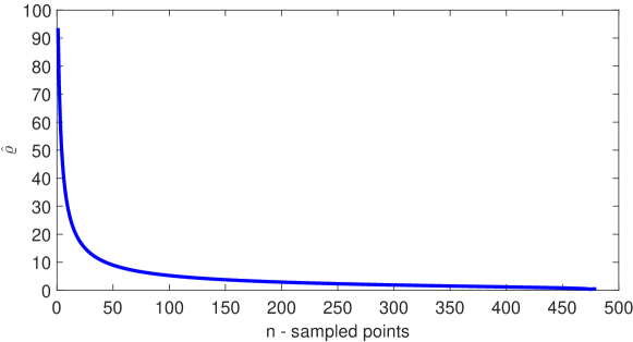
Figure 2: Values of $\hat{\varrho}$ versus number of sampled points $n$ for $K=3$ clusters generated by (22) with $D=1$, cluster means $\{0,0.5,1\}$, variances $\{0.3,0.3,0.3\}$, and number of points per cluster $\{100,180,200\}$.

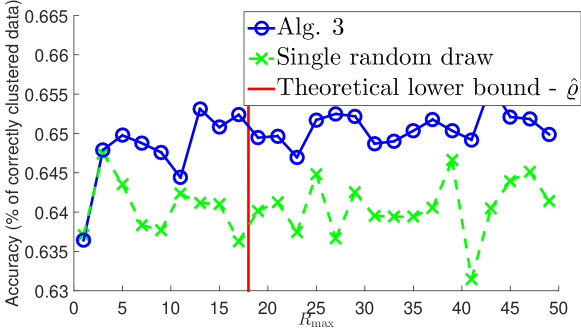
Figure 3: Accuracy (% of correctly clustered data) versus $R_{\max}$ number of sampled points $n$ for the data used in Fig. 2. Alg. 3 is compared to the simple scheme of taking a single random draw of $n$ data, followed by clustering. The vertical line represents the $\hat{\varrho}$ value given by Theorem 1.

When reliable estimates of $f$ are unknown, values for $R_{\max}$ can be estimated on-the-fly using (26) and sample averaging. The ensemble averages of Thm. 1.1 can be replaced by sampled ones, where averaging takes place across iterations. Specifically, $\operatorname{\mathbb{E}}[d(\hat{f},f_{0})]$ [cf. (26)] is replaced by $\bar{d}^{(r)}(\hat{f},f_{0})$, which denotes the running sample average of $d(\hat{f},f_{0})$, as of realization $r$. Moreover, since the number $n^{\prime}$ of data used in the validation phase is set to be larger than or equal to the number $n$ of data drawn in the sketching phase of Alg. 3, $\tilde{f}$ of (20c) provides potentially better estimates of $f$ than $\hat{f}$ does. As a result, distance $d(\tilde{f}^{(i)},f_{0}^{(i)})$ can be employed as a surrogate to $\delta^{\prime}$ [cf. (23)]. Further, by $d:=\sqrt{d_{\text{ISE}}}$ and by using (44), (55), as well as replacing ensemble with sample averages, an estimate of $\delta_{0}$ at realization $r$ of Alg. 3 is

$$\bar{\delta}_{0}^{(r)}:=\left(\sqrt{-\frac{2\log(q/2)}{nh\left(4\pi\right)^{D/2}}}+\bar{d}^{(r)}(\tilde{f},\hat{f})+\bar{d}^{(r)}(\tilde{f},f_{0})\right)^{2}$$ (35)

where $\bar{d}^{(r)}(\tilde{f},\hat{f})$ and $\bar{d}^{(r)}(\tilde{f},f_{0})$ are the sample averages of $d(\tilde{f},\hat{f})$ and $d(\tilde{f},f_{0})$, respectively. Therefore, according to (20), the following quantities can be computed per realization of Alg. 3:

$$\bar{d}^{(r)}(f_{0},\hat{f})=\frac{1}{r}\sum_{i=1}^{r}d(f_{0}^{(i)},\hat{f}^{(i)})=\frac{r-1}{r}\bar{d}^{(r-1)}(f_{0},\hat{f})+\frac{1}{r}d(f_{0}^{(r)},\hat{f}^{(r)})$$ (36a)

$$\bar{d}^{(r)}(\tilde{f},\hat{f})=\frac{1}{r}\sum_{i=1}^{r}d(\tilde{f}^{(i)},\hat{f}^{(i)})=\frac{r-1}{r}\bar{d}^{(r-1)}(\tilde{f},\hat{f})+\frac{1}{r}d(\tilde{f}^{(r)},\hat{f}^{(r)})$$ (36b)

$$\bar{d}^{(r)}(\tilde{f},f_{0})=\frac{1}{r}\sum_{i=1}^{r}d(\tilde{f}^{(i)},f_{0}^{(i)})=\frac{r-1}{r}\bar{d}^{(r-1)}(\tilde{f},f_{0})+\frac{1}{r}d(\tilde{f}^{(r)},f_{0}^{(r)})\,.$$ (36c)

Consequently, (26) can be approximated per iteration $r$ using (35) and (36a)-(36c) as

$$\boxed{\hat{R}_{\max}^{(r)}\geq\frac{\log(1-p)}{\log\left(1-\frac{\bar{d}^{(r)}(f_{0},\hat{f})}{\bar{\delta}_{0}^{(r)}}\right)}=:\bar{\varrho}^{(r)}.}$$ (37)

Based on the previous sample averages, a simple rule for updating $\hat{R}^{(r)}_{\max}$, which quantifies the maximum number of iterations to be executed in Alg. 3, as of iteration $r$, is

$$\hat{R}^{(r)}_{\max}:=\max\left\{\bar{\varrho}^{(r)},R_{0}\right\}$$ (38)

where $R_{0}$ is a prescribed absolute minimum number of iterations. Fig. 4 shows the values of (38) as iterations of Alg. 3 are run for the dataset used in Figs. 2 and 3. Here $R_{0}:=3$, and $\hat{R}_{\max}^{(r)}$ approaches the theoretical value given by Thm. 1, as values of the distances are averaged across iterations.

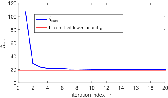
Figure 4: Estimates $\hat{R}^{(r)}_{\max}$ [cf. (38)] versus iteration index for a dataset with $K=3$ clusters generated by (22) with $D=1$, cluster means $\{0,0.5,1\}$, variances $\{0.3,0.3,0.3\}$, and number of points per cluster $\{100,180,200\}$. The horizontal line represents the $\hat{\varrho}$ value given by Theorem 1 when $f$ is known.

5 Numerical Tests

The proposed algorithm is validated using synthetic and real datasets. SkeVa-SC is compared to SSSC, which is the state-of-the-art algorithm for scalable SC. The metrics evaluated are:

• Accuracy, i.e., percentage of correctly clustered data:

  $$\text{Accuracy}:=\frac{\text{\# of data correctly clustered}}{N}\,.$$

• Normalized mutual information (NMI) [38] between experimental and the ground truth labels:

  $$\text{NMI}:=\frac{I(\varPi;\varPi^{\prime})}{\max\{\mathcal{H}(\varPi),\mathcal{H}(\varPi^{\prime})\}}$$

  where $\varPi$ is a random variable taking values $\{1,2,\ldots,K\}$ with probabilities $p(\pi_{k})=\Pr\left(\varPi=k\right)={N_{k}}/{N}$ of a datum to belong to cluster $k$. Here $N_{k}$ is the number of data in cluster $k$, and its value is provided by the algorithms tested. Quantity $\varPi^{\prime}$ is a random variable identical to $\varPi$, but with probabilities derived by the ground-truth labels, while $I(\varPi;\varPi^{\prime})$ is the mutual information between the random variables $\varPi$ and $\varPi^{\prime}$ [34]:

  $$I(\varPi;\varPi^{\prime}):=\sum_{i,j}p(\pi_{i},\pi_{j}^{\prime})\log\frac{p(\pi_{i},\pi_{j}^{\prime})}{p(\pi_{i})p(\pi_{j}^{\prime})}\,,$$

  where $\mathcal{H}(\varPi)$ denotes the entropy of $\varPi$ defined as [34]

  $$\mathcal{H}(\varPi):=-\sum_{i}p(\pi_{i})\log p(\pi_{i})\,.$$

• Time (in seconds) required for clustering all data.

The bandwidth matrix used for Alg. 3 is $\mathbf{H}:=h^{2}(C,n)\mathbf{I}_{D}$ with $h$ similar to that in (13), where the unknown quantity pertaining to the curvature of $f$ is replaced by a user-defined constant $C$; that is

$$h(C,n):=\left[\frac{CD\phi_{2\mathbf{I}}(\bm{0})}{n}\right]^{1/(D+4)}=\left[\frac{CD}{n\left(4\pi\right)^{D/2}}\right]^{1/(D+4)}\,.$$ (39)

Furthermore, the scoring function $\psi$ used in Alg. 3 is $\psi(x):=x^{-1}$. The software used to conduct all experiments is MATLAB [39]. All results represent the averages of $10$ independent Monte Carlo runs.

5.1 Synthetic data

Tests on synthetic datasets of dimensions $D=100$ and $D=500$ with $K=5$ subspaces are shown in Figs. 5 and 6, respectively. Subspaces have dimensions $\{12,10,5,3,2\}$, and the number of data per subspace is proportional to the subspace dimension: $N_{k}:=200d_{k}$. The data per subspace have been generated according to (1), where $\{\bm{m}_{k}=\bm{0}\}_{k=1}^{K}$, the subspace bases $\{\mathbf{U}_{k}\}_{k=1}^{K}$ are randomly generated so that the subspace angle $\eta(i,j)$ between $\mathcal{S}_{i},\mathcal{S}_{j}$ given by

$$\eta(i,j):=\min_{\bm{u},\bm{v}}\left\{\operatorname{arc}\cos\left(\frac{|\bm{u}^{\top}\bm{v}|}{\|\bm{u}\|\|\bm{v}\|}\right):\bm{u}\in{\mathcal{S}}_{i},\bm{v}\in{\mathcal{S}}_{j}\right\}$$

is at least $\pi/4$, $\forall(i,j)\in\{1,\ldots,K\}^{2}$, $i\neq j$. Projections $\bm{y}_{i}$ of $\bm{x}_{i}$’s onto their subspaces are also randomly drawn from a uniform distribution on the volume of the unit $d_{k}$-dimensional hypercube: $\bm{y}_{i}\sim\mathcal{U}[-1,1]^{d_{k}}$, where $\mathcal{U}$ denotes uniform distribution. Finally, AWGN with variance $\sigma^{2}=0.1$ is added to all data: $\bm{v}_{i}\sim\mathcal{N}(\bm{0},\sigma^{2}\mathbf{I}_{D})$. The number of points for the validation stage of Alg. 3 is $n^{\prime}=600$ and the maximum number of iterations is set to $R_{\max}=100$. As the number of sampled data $n$ increases, so does the clustering accuracy, as well as the normalized mutual information (NMI) between the cluster assignments and the ground truth ones. Both of these metrics for the proposed method are larger than those of SSSC, corroborating the fact that a single random sketch (SSSC) may not be representative of the data to ensure reliable clustering. Additionally, required processing times by SSSC and SkeVa-SC are comparable.

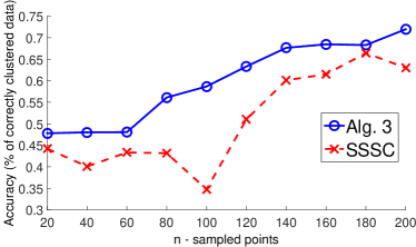
(a) Clustering accuracy

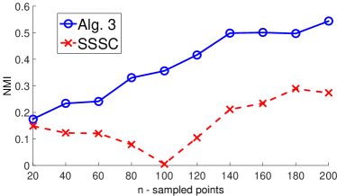
(b) NMI

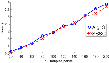
(c) Clustering time (seconds)

Figure 5: Simulated tests on a synthetic dataset with $K=5$ subspaces, $D=100$ and $N=6,400$ data.

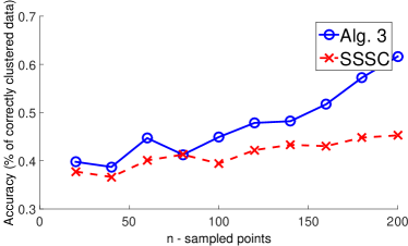
(a) Clustering accuracy

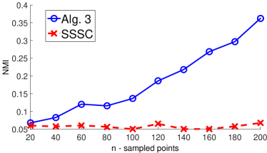
(b) NMI

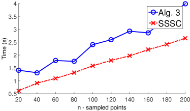
(c) Clustering time (seconds)

Figure 6: Simulated tests on a synthetic dataset with $K=5$ subspaces, $D=500$ and $N=6,400$ data.

5.2 Real data

The real datasets tested are the PenDigits [40], the Extended Yale Face  [41], and the PokerHand UCI [42] databases. The PenDigits dataset includes $N=10,992$ data of dimension $D=16$, separated into $K=10$ clusters, with each datum representing a handwritten digit. Clusters group same digits, and each cluster contains $N_{k}=250$ data.

The results for the PenDigits dataset are shown in Fig. 7, with $C=10^{-3}$ [cf. (39)], $\mathbf{H}=h^{2}(C,n)\mathbf{I}_{D},\mathbf{H}_{0}=({h^{2}(C,n)}/{4})\mathbf{I}_{D},\mathbf{H}^{\prime}=h^{2}(C,n^{\prime})\mathbf{I}_{D}$, $n^{\prime}=700$, and $R_{\max}=150$. Similar to the synthetic tests, as the number of data increases so does the accuracy and NMI of both Alg. 3 and SSSC, with Alg. 3 showing higher accuracy and NMI levels at the cost of higher computational time. The accuracy and NMI difference between SSSC and Alg. 3 is not as pronounced as in the synthetic datasets, possibly because the PenDigits dataset is uniform, that is all clusters have the same number of data.

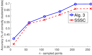
(a) Clustering accuracy

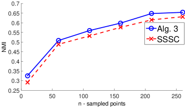
(b) NMI

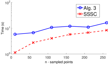
(c) Clustering time (seconds)

Figure 7: Simulated tests on real dataset PenDigits, with $N=10,992$ data dimension $D=16$ and $K=10$ clusters.

The Extended Yale Face database contains $N=2,414$ face images of $K=38$ people, each of dimension $D=2,016$. The dimensionality of the data was reduced using PCA by extracting the $114$ most important features and Alg. 3 and SSSC were tested on the dimensionality reduced and normalized data. Fig. 8 shows the results for this dataset, with $C=10^{-2}$, $\mathbf{H}=h^{2}(C,n)\mathbf{I}_{D},\mathbf{H}_{0}=({h^{2}(C,n)}/{4})\mathbf{I}_{D},\mathbf{H}^{\prime}={h^{2}(C,n^{\prime})}\mathbf{I}$, $n^{\prime}=700$, and $R_{\max}=150$. Again Alg. 3 exhibits higher accuracy and NMI than its one-shot random sampling counterpart SSSC at basically comparable clustering time.

Furthermore, Figs. 9a and 9b show accuracy and time results for the Yale Face database when the maximum number of iterations is estimated on-the-fly, as described in Section 4, using (26) after replacing the ensemble averages with sample averages across iterations. Fig. 9c shows the values of $\hat{R}_{\max}$ versus the number of sampled data. Here $C=1$, $\mathbf{H}=h^{2}(C,n)\mathbf{I}_{D},\mathbf{H}_{0}=({h^{2}(C,n)}/{4})\mathbf{I}_{D},\mathbf{H}^{\prime}=({h(C,n^{\prime})})^{2}\mathbf{I}$, $n^{\prime}=600$, $p=0.99$ and $q=0.01$. Similarly to the prescribed $R_{\max}$ case Alg. 3 exhibits higher clustering accuracy while requiring comparable running time as SSSC.

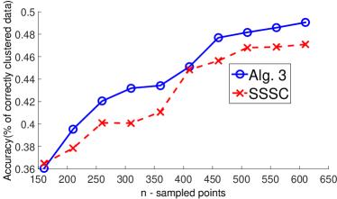
(a) Clustering accuracy

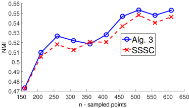
(b) NMI

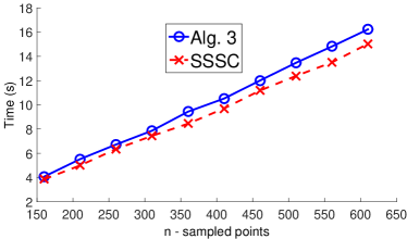
(c) Clustering time (seconds)

Figure 8: Simulated tests on real dataset Extended Yale Face Database B, with $N=2,414$ data dimension $D=114$ and $K=38$ clusters.

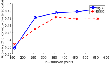
(a) Clustering accuracy

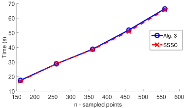
(b) Clustering time (seconds)

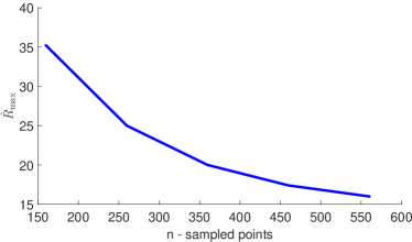
(c) $\hat{R}_{\max}$

Figure 9: Simulated tests on real dataset Extended Yale Face Database B, with $N=2,414$ data dimension $D=114$ and $K=38$ clusters.

The PokerHand database contains $N=10^{6}$ data, belonging to $K=10$ clusters. Each datum is a $5$-card hand drawn from a deck of $52$ cards, with each card being described by its suit (spades, hearts, diamonds, and clubs) and rank. Each cluster represents a valid Poker hand. Fig. 10 compares SkeVa-SC with SSSC on this dataset after selecting $C=10^{-2}$, $\mathbf{H}=h^{2}(C,n)\mathbf{I}_{D},\mathbf{H}_{0}=({h^{2}(C,n)}/{4})\mathbf{I}_{D},\mathbf{H}^{\prime}=h^{2}(C,n^{\prime})\mathbf{I}_{D}$, $n^{\prime}=800$, and $R_{\max}=150$. Similar to the previous datasets, Alg. 3 enjoys higher accuracy than SSSC, while retaining low clustering time, corroborating the fact that Alg. 3 can handle very large datasets. However, NMI is at suprisingly low levels, for both algorithms.

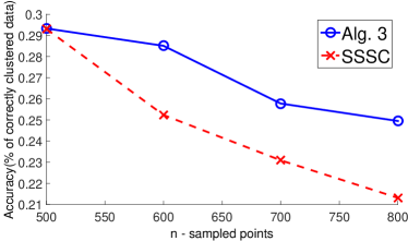
(a) Clustering accuracy

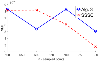
(b) NMI

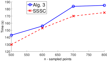
(c) Clustering time (seconds)

Figure 10: Simulated tests on real dataset Pokerhand, with $N=10^{6}$ data dimension $D=10$ and $K=10$ clusters.

6 Conclusions and future work

The present paper introduced a novel iterative data-reduction scheme, SkeVa-SC, that enables grouping of data drawn from a union of subspaces based on a random sketching and validation approach for fast, yet-accurate subspace clustering (SC). Part of the proposed algorithm builds on the sparse SC algorithm, but it can also utilize any other SC algorithm. Analytical bounds were derived on the number of required iterations, and performance of the algorithm was evaluated on synthetic and real datasets. Future research directions will focus on the development of online SkeVa-SC, able to handle not only big, but also fast-streaming data.

Appendix A Integrated square error performance

Using the definition of $d$, $\forall f,g\in\mathcal{X}$, we have

$$d(f,g):=\sqrt{d_{\text{ISE}}(f,g)}:=\sqrt{\int\left(f(\bm{x})-g(\bm{x})\right)^{2}d\bm{x}}\,.$$ (40)

Based on (40), the concavity of $\sqrt{\cdot}$, and Jensen’s inequality [34], an upper bound on $\operatorname{\mathbb{E}}[d(\cdot,\cdot)]$ is

$$\operatorname{\mathbb{E}}[d(\cdot,\cdot)]=\operatorname{\mathbb{E}}\left[\sqrt{d_{\text{ISE}}(\cdot,\cdot)}\right]\leq\sqrt{\operatorname{\mathbb{E}}\left[d_{\text{ISE}}(\cdot,\cdot)\right]}=\sqrt{\operatorname{\mathbb{E}}\left[d^{2}(\cdot,\cdot)\right]}$$ (41)

and consequently, $\operatorname{\mathbb{E}}^{2}[d(\cdot,\cdot)]\leq\operatorname{\mathbb{E}}[d^{2}(\cdot,\cdot)]$.

To ensure positivity, the number of required iterations of (31) can be rewritten as

$$R_{\max}\geq\frac{\log(\frac{1}{1-p})}{\log(\frac{1}{\Pr(\mathcal{B}_{\delta})})}.$$ (42)

Thus, for a fixed $p$ the lower bound on the number of required iterations grows as the probability of a “bad” event (as defined in Def. 2) increases.

The bad event probability of (32) can be lower-bounded using the extended Markov inequality for the quadratic function in $\mathbb{R}_{+}$, namely

$$\operatorname{Pr}(\mathcal{B}_{\delta})\geq 1-\frac{\operatorname{\mathbb{E}}\left[d^{2}(\hat{f},f_{0})\right]}{\delta_{0}^{2}}\,.$$ (43)

For $\operatorname{\mathbb{E}}[d^{2}(\hat{f},f_{0})]$ fixed, the larger $\delta_{0}$ the larger the lower bound on the probability of $\mathcal{B}_{\delta}$ becomes, and consequently the lower bound on $R_{\max}$ increases.

Based on (33), define $\delta_{0}:=d(f_{0},\hat{f})$, which is a random variable given its dependence on $\hat{f}$. By the triangle inequality, $\delta_{0}$ can be bounded as

$$|\delta^{\prime}-d(f,\hat{f})|\leq\delta_{0}\leq d(f,\hat{f})+\delta^{\prime}\,.$$ (44)

The upper bound of (44) will be used to provide a data-driven and relatively “safe” lower bound on the probability of $\mathcal{B}_{\delta}$, using the aforementioned observations. While $d(f,\hat{f})$ is a quantity that depends on $\hat{f}$, and it is thus random, it will be further bounded by deterministic quantities, yielding a deterministic bound on $\delta_{0}$.

Distance $\delta^{\prime}:=d(f,f_{0})$ can be expressed in closed form using (As. 1) and property (12) as

$$\delta^{\prime 2} = \;d^{2}(f,f_{0})=\int\left(f(\bm{x})-f_{0}(\bm{x})\right)^{2}d\bm{x}=\int f^{2}(\bm{x})d\bm{x}+\int f_{0}^{2}(\bm{x})d\bm{x}-2\int f(\bm{x})f_{0}(\bm{x})d\bm{x}$$

$$= \int\sum_{\ell}\sum_{\ell^{\prime}}w_{\ell}w_{\ell^{\prime}}\phi_{\mathbf{\Sigma}_{\ell}}(\bm{\mu}_{\ell}-\bm{x})\phi_{\mathbf{\Sigma}_{\ell^{\prime}}}(\bm{\mu}_{\ell^{\prime}}-\bm{x})+\int\phi_{\mathbf{H}_{0}}(\bm{\mu}_{0}-\bm{x})\phi_{\mathbf{H}_{0}}(\bm{\mu}_{0}-\bm{x})$$

$$-2\int\sum_{\ell}w_{l}\phi_{\mathbf{\Sigma}_{\ell}}(\bm{\mu}_{\ell}-\bm{x})\phi_{\mathbf{H}_{0}}(\bm{\mu}_{0}-\bm{x})$$

$$= \;\mathbf{w}^{\top}\mathbf{\Omega}_{0}\mathbf{w}+\frac{1}{(4\pi)^{D/2}|\mathbf{H}_{0}|^{1/2}}-2\sum_{\ell}w_{\ell}\phi_{\mathbf{\Sigma}_{\ell}+\mathbf{H}_{0}}(\bm{\mu}_{\ell}-\bm{\mu_{0}})$$ (45)

where $\mathbf{w}:=[w_{1},w_{2},\ldots,w_{L}]^{\top}$ is formed by the mixing coefficients of (22), and $|\mathbf{H}|$ denotes the determinant of $\mathbf{H}$. Distances $d(\hat{f},f)$ and $d(\hat{f},f_{0})$ are random variables since they depend on $\hat{f}$, which in turn depends on the randomly drawn data $\bm{x}_{i}$. Due to (As. 1), their expectation w.r.t. the true data pdf $f$ can be expressed in closed form. As data are drawn independently per iteration $r$, expectations do not depend on $r$. As such, we have

$$\operatorname{\mathbb{E}}[d^{2}(\hat{f},f_{0})] =\; \operatorname{\mathbb{E}}[d_{\text{ISE}}(\hat{f},f_{0})]=\operatorname{\mathbb{E}}\left[\int\left(\hat{f}(\bm{x})-f_{0}(\bm{x})\right)^{2}d\bm{x})\right]\hskip 100.0pt$$

$$= \int f_{0}^{2}(\bm{x})d\bm{x}+\operatorname{\mathbb{E}}\left[\int\hat{f}^{2}(\bm{x})d\bm{x}\right]-2\operatorname{\mathbb{E}}\left[\int f_{0}(\bm{x})\hat{f}(\bm{x})d\bm{x}\right]$$

$$= \frac{1}{(4\pi)^{D/2}|\mathbf{H}_{0}|^{1/2}}+\int\operatorname{\mathbb{E}}\left[\hat{f}^{2}(\bm{x})d\bm{x}\right]-2\operatorname{\mathbb{E}}\left[\int f_{0}(\bm{x})\hat{f}(\bm{x})d\bm{x}\right]$$

$$= \frac{1}{(4\pi)^{D/2}|\mathbf{H}_{0}|^{1/2}}+\frac{1}{n}\frac{1}{(4\pi)^{D/2}|\mathbf{H}|^{1/2}}+\left(1-\frac{1}{n}\right)\mathbf{w}^{\top}\mathbf{\Omega}_{2}\mathbf{w}-2\sum_{\ell}w_{\ell}\phi_{\mathbf{H}+\mathbf{H}_{0}+\mathbf{\Sigma}_{\ell}}(\bm{\mu}_{\ell}-\bm{\mu}_{0})$$ (46)

and

$$\operatorname{\mathbb{E}}[d^{2}(\hat{f},f)]=\;\operatorname{\mathbb{E}}[d_{\text{ISE}}(\hat{f},f)]=\;\frac{1}{n(4\pi)^{D/2}|\mathbf{H}|^{1/2}}+\mathbf{w}^{\top}\left(\left(1-\frac{1}{n}\right)\mathbf{\Omega}_{2}-2\mathbf{\Omega}_{1}+\mathbf{\Omega}_{0}\right)\mathbf{w}$$ (47)

with

$$\int\operatorname{\mathbb{E}}[\hat{f}^{2}(\bm{x})]d\bm{x} = \;\int\frac{1}{n^{2}}\sum_{i}\sum_{j}\operatorname{\mathbb{E}}\left[\phi_{\mathbf{H}}(\bm{x}-\bm{x}_{i})\phi_{\mathbf{H}}(\bm{x}-\bm{x}_{j})\right]d\bm{x}$$

$$= \;\int\left\{\frac{1}{n^{2}}\sum_{i=j}\operatorname{\mathbb{E}}\left[\phi_{\mathbf{H}}^{2}(\bm{x}-\bm{x}_{i})\right]\right.\left.+\frac{1}{n^{2}}\sum_{i\neq j}\operatorname{\mathbb{E}}\left[\phi_{\mathbf{H}}(\bm{x}-\bm{x}_{i})\phi_{\mathbf{H}}(\bm{x}-\bm{x}_{j})\right]\right\}d\bm{x}$$

$$= \;\int\left\{\frac{1}{n}\operatorname{\mathbb{E}}\left[\phi_{\mathbf{H}}^{2}(\bm{x}-\bm{x}_{i})\right]\right.\left.+\frac{n^{2}-n}{n^{2}}\operatorname{\mathbb{E}}^{2}\left[\phi_{\mathbf{H}}(\bm{x}-\bm{x}_{i})\right]\right\}d\bm{x}$$

$$= \;\frac{1}{n}\frac{1}{\left(4\pi\right)^{D/2}|\mathbf{H}|^{1/2}}+\left(1-\frac{1}{n}\right)\mathbf{w}^{\top}\mathbf{\Omega}_{2}\mathbf{w}$$ (48)

where the third equality is due to the fact that $\bm{x}_{i}$’s are independently drawn from $f$. Moreover,

$$\operatorname{\mathbb{E}}\left[\int f_{0}(\bm{x})\hat{f}(\bm{x})d\bm{x}\right] =\frac{1}{n}\operatorname{\mathbb{E}}\left[\sum_{i}\int\phi_{\mathbf{H}_{0}}(\bm{x}-\bm{\mu}_{0})\phi_{\mathbf{H}}(\bm{x}-\bm{x}_{i})d\bm{x}\right]=\frac{1}{n}\operatorname{\mathbb{E}}\left[\sum_{i}\phi_{\mathbf{H}+\mathbf{H}_{0}}(\bm{x}_{i}-\bm{\mu}_{0})\right]$$

$$=\operatorname{\mathbb{E}}\left[\phi_{\mathbf{H}+\mathbf{H}_{0}}(\bm{x}-\bm{\mu}_{0})\right]=\int\sum_{\ell}w_{\ell}\phi_{\mathbf{\Sigma}_{\ell}}(\bm{x}-\bm{\mu}_{\ell})\phi_{\mathbf{H}+\mathbf{H}_{0}}(\bm{x}-\bm{\mu}_{0})d\bm{x}$$

$$=\sum_{\ell}w_{\ell}\phi_{\mathbf{H}+\mathbf{H}_{0}+\mathbf{\Sigma}_{\ell}}(\bm{\mu}_{\ell}-\bm{\mu}_{0})\,.$$ (49)

Interestingly, the probability of $d(f,\hat{f})$ being far from its ensemble average $\operatorname{\mathbb{E}}[d(f,\hat{f})]$ can be bounded via the general inequality [43]

$$\Pr\left(\left|\|f-\hat{f}\|_{p}-\operatorname{\mathbb{E}}\left[\|f-\hat{f}\|_{p}\right]\right|\geq t\right)\leq 2\exp\left(-\frac{nt^{2}h^{2-2/p}}{2\|K_{\mathbf{I}}(\bm{x})\|_{p}^{2}}\right)$$ (50)

where $\|\cdot\|_{p}$ denotes the $L_{p}$-norm for $p\geq 1$, i.e., $\|f\|_{p}:=\left(\int|f(x)|^{p}dx\right)^{1/p}$. For the Gaussian kernel with covariance matrix $\mathbf{H}:=h^{2}\mathbf{I}_{D}$ and $p=2$, the norm $\|K_{\mathbf{I}}(\bm{x})\|_{2}^{2}$ becomes

$$\|K_{\mathbf{I}}(\bm{x})\|_{2}^{2}=\|\phi_{\mathbf{I}}(\bm{x})\|_{2}^{2}=\int\phi_{\mathbf{I}}^{2}(\bm{x})d\bm{x}=\phi_{2\mathbf{I}}(\bm{0})=\frac{1}{(4\pi)^{D/2}}\,.$$ (51)

Consequently, (50) reduces to

$$\Pr\left(\left|d(f,\hat{f})-\operatorname{\mathbb{E}}\left[d(f,\hat{f})\right]\right|\geq t\right)\leq 2\exp\left(-\frac{nt^{2}h\left(4\pi\right)^{D/2}}{2}\right)\,.$$ (52)

Letting $q:=\Pr(|d(f,\hat{f})-\operatorname{\mathbb{E}}[d(f,\hat{f})]|\geq t)$, (52) yields

$$q\leq 2\exp\left(-\frac{nt^{2}h\left(4\pi\right)^{D/2}}{2}\right)$$ (53)

and solving (53) w.r.t. $t$, we arrive at

$$t\leq\sqrt{-\frac{2\log(q/2)}{nh\left(4\pi\right)^{D/2}}}\,.$$ (54)

Since $1-q=\Pr(|d(f,\hat{f})-\operatorname{\mathbb{E}}[d(f,\hat{f})]|<t)$, the distance $d(f,\hat{f})$ can be upper bounded with probability $1-q$ as

$$d(f,\hat{f})<\sqrt{-\frac{2\log(q/2)}{nh\left(4\pi\right)^{D/2}}}+\operatorname{\mathbb{E}}[d(f,\hat{f})]\leq\sqrt{-\frac{2\log(q/2)}{nh\left(4\pi\right)^{D/2}}}+\sqrt{\operatorname{\mathbb{E}}[d^{2}(f,\hat{f})]}$$ (55)

where the second inequality follows readily from (41).

An upper bound with probability $1-q$ to obtain the value of $\delta_{0}$ can be now derived using (44) and (55):

$$\delta_{0}\leq d(f,\hat{f})+\delta^{\prime}\leq\sqrt{-\frac{2\log(q/2)}{nh\left(4\pi\right)^{D/2}}}+\sqrt{\operatorname{\mathbb{E}}[d^{2}(f,\hat{f})]}+\delta^{\prime}=:\theta.$$ (56)

Using $\theta$ in place of $\delta_{0}$ will yield an increased lower bound to $R_{\max}$, as it will increase the value of $1-\operatorname{\mathbb{E}}[d^{2}(\hat{f},f_{0})]/\delta_{0}^{2}$, in (43); thus, with probability $1-q$

$$1-\frac{\operatorname{\mathbb{E}}\left[d^{2}(\hat{f},f_{0})\right]}{\left(\delta^{\prime}+\sqrt{-\frac{2\log(q/2)}{nh\left(4\pi\right)^{D/2}}}+\sqrt{\operatorname{\mathbb{E}}[d^{2}(f,\hat{f})]}\right)^{2}}\geq 1-\frac{\operatorname{\mathbb{E}}\left[d^{2}(\hat{f},f_{0})\right]}{\delta_{0}^{2}}\,.$$ (57)

Finally, using (57), an overestimate $\hat{\varrho}$, with probability $1-q$, of the lower bound $\varrho$ in (27) is

$$\hat{\varrho}:=\frac{\log(1-p)}{\log\left(1-\frac{\operatorname{\mathbb{E}}\left[d^{2}(\hat{f},f_{0})\right]}{\left(\delta^{\prime}+\sqrt{-\frac{2\log(q/2)}{nh\left(4\pi\right)^{D/2}}}+\sqrt{\operatorname{\mathbb{E}}[d^{2}(f,\hat{f})]}\right)^{2}}\right)}.$$ (58)

Upon $\theta_{1}:=(-{2\log(q/2)}/{(nh(4\pi)^{D/2})})^{1/2}+(\operatorname{\mathbb{E}}[d^{2}(f,\hat{f})])^{1/2}$, and $\theta_{2}:=\delta^{\prime}$, the claim of Thm. 1.2 is established.

References

- [1] K. Cukier, “Data, data everywhere,” The Economist, 2010. [Online]. Available: http://www.economist.com/node/15557443
- [2] G. O’ Connor. (2014) Moore’s law gives way to Bezos’ law. [Online]. Available: https://gigaom.com/2014/04/19/moores-law-gives-way-to-bezoss-law/
- [3] C. M. Bishop, Pattern Recognition and Machine Learning. Springer, 2006.
- [4] T. Hastie, R. Tibshirani, and J. Friedman, The Elements of Statistical Learning. New York: Springer, 2001.
- [5] R. Vidal, “A tutorial on subspace clustering,” IEEE Signal Process. Magazine, vol. 28, no. 2, pp. 52–68, 2010.
- [6] P. A. Traganitis, K. Slavakis, and G. B. Giannakis, “Sketch and validate for big data clustering,” IEEE J. Selected Topics Signal Processing, vol. 9, no. 4, pp. 678–690, June 2015.
- [7] M. Fisher and R. Bolles, “Random sample consensus: A paradigm for model fitting with applications to image analysis and automated cartography,” Comm. ACM, vol. 24, pp. 381–395, June 1981.
- [8] M. P. Wand and M. C. Jones, Kernel Smoothing. CRC Press, 1994.
- [9] J. Park and I. W. Sandberg, “Universal approximation using radial-basis-function networks,” Neural Computation, vol. 3, no. 2, pp. 246–257, 1991.
- [10] C. E. Rasmussen and C. K. I. Williams, Gaussian Processes for Machine Learning. MIT Press, 2006.
- [11] P. K. Agarwal and N. H. Mustafa, “-means projective clustering,” in Proc. 23rd ACM SIGMOD-SIGACT-SIGART Symposium. Paris, France: ACM, June 2004, pp. 155–165.
- [12] S. Lloyd, “Least-squares quantization in PCM,” IEEE Trans. Info. Theory, vol. 28, no. 2, pp. 129–137, 1982.
- [13] I. Jolliffe, Principal Component Analysis. Wiley Online Library, 2002.
- [14] L. Parsons, E. Haque, and H. Liu, “Subspace clustering for high dimensional data: A review,” ACM SIGKDD Explorations Newsletter, vol. 6, no. 1, pp. 90–105, 2004.
- [15] M. Tipping and C. Bishop, “Mixtures of probabilistic principal component analyzers,” Neural Computation, vol. 11, no. 2, pp. 443–482, 1999.
- [16] Y. Ma, H. Derksen, W. Hong, and J. Wright, “Segmentation of multivariate mixed data via lossy data coding and compression,” IEEE Trans. Pattern Analysis Machine Intelligence, vol. 29, no. 9, pp. 1546–1562, 2007.
- [17] T. Berger, “Rate-distortion theory,” Encyclopedia of Telecommunications, 1971.
- [18] J. P. Costeira and T. Kanade, “A multibody factorization method for independently moving objects,” Intern. J. Computer Vision, vol. 29, no. 3, pp. 159–179, 1998.
- [19] R. Vidal, Y. Ma, and S. Sastry, “Generalized principal component analysis (gpca),” IEEE Trans. Pattern Analysis Machine Intelligence, vol. 27, no. 12, pp. 1945–1959, 2005.
- [20] T. Zhang, A. Szlam, Y. Wang, and G. Lerman, “Hybrid linear modeling via local best-fit flats,” Intern. J. Computer Vision, vol. 100, no. 3, pp. 217–240, 2012.
- [21] T. Zhang, A. Szlam, and G. Lerman, “Median -flats for hybrid linear modeling with many outliers,” in Proc. of ICCV. Kyoto, Japan: IEEE, September 2009, pp. 234–241.
- [22] R. Vidal, “Online clustering of moving hyperplanes,” in Advances in Neural Information Processing Systems, Vancouver, Canada, December 2006, pp. 1433–1440.
- [23] U. Von Luxburg, “A tutorial on spectral clustering,” Statistics and Computing, vol. 17, no. 4, pp. 395–416, 2007.
- [24] E. Elhamifar and R. Vidal, “Sparse subspace clustering: Algorithm, theory, and applications,” IEEE Trans. Pattern Analysis Machine Intelligence, vol. 35, no. 11, pp. 2765–2781, 2013.
- [25] G. Liu, Z. Lin, and Y. Yu, “Robust subspace segmentation by low-rank representation,” in Proc. ICML, Haifa, Israel, June 2010, pp. 663–670.
- [26] C. Boutsidis, A. Zouzias, M. W. Mahoney, and P. Drineas, “Randomized dimensionality reduction for k-means clustering,” Information Theory, IEEE Transactions on, vol. 61, no. 2, pp. 1045–1062, 2015.
- [27] X. Peng, L. Zhang, and Z. Yi, “Scalable sparse subspace clustering,” in Proc. CVPR, Portland, OR, USA, June 2013, pp. 430–437.
- [28] P. Hall, “Large sample optimality of least squares cross-validation in density estimation,” Annals Statistics, pp. 1156–1174, 1983.
- [29] D. W. Scott and G. R. Terrell, “Biased and unbiased cross-validation in density estimation,” J. American Statistical Association, vol. 82, no. 400, pp. 1131–1146, 1987.
- [30] S. J. Sheather and M. C. Jones, “A reliable data-based bandwidth selection method for kernel density estimation,” J. Royal Statistical Society (Series B), pp. 683–690, 1991.
- [31] P. Hall, J. S. Marron, and B. U. Park, “Smoothed cross-validation,” Probability Theory and Related Fields, vol. 92, no. 1, pp. 1–20, 1992.
- [32] J. Dean and S. Ghemawat, “MapReduce: Simplified data processing on large clusters,” Comm. ACM, vol. 51, no. 1, pp. 107–113, 2008.
- [33] J. C. Principe, Information Theoretic Learning: Renyi’s Entropy and Kernel Perspectives. Springer, 2010.
- [34] T. M. Cover and J. A. Thomas, Elements of Information Theory. John Wiley & Sons, 2012.
- [35] F. Itakura and S. Saito, “Analysis synthesis telephony based on the maximum likelihood method,” in Proc. Intern. Congress Acoustics, vol. 17, Tokyo, Japan, August 1968, pp. C17–C20.
- [36] S. Acharyya, A. Banerjee, and D. Boley, “Bregman divergences and triangle inequality.” in Proc. of SDM. Austin, TX, USA: SIAM, May 2013, pp. 476–484.
- [37] S. I. Amari, O. E. Barndorff-Nielsen, R. E. Kass, S. L. Lauritzen, and C. R. Rao, “Differential geometry in statistical inference,” Lecture Notes-Monograph Series, pp. i–240, 1987.
- [38] D. Cai, X. He, and J. Han, “Document clustering using locality preserving indexing,” IEEE Trans. Knowledge Data Engineering, vol. 17, no. 12, pp. 1624–1637, Dec 2005.
- [39] MATLAB, version 8.4.0 (R2014b). Natick, Massachusetts: The MathWorks Inc., 2014.
- [40] F. Alimoglu and E. Alpaydin, “Methods of combining multiple classifiers based on different representations for pen-based handwritten digit recognition,” in Proc. of TAINN, Istanbul, Turkey, 1996.
- [41] A. S. Georghiades, P. N. Belhumeur, and D. J. Kriegman, “From few to many: Illumination cone models for face recognition under variable lighting and pose,” IEEE Trans. Pattern Analysis Machine Intelligence, vol. 23, no. 6, pp. 643–660, June 2001.
- [42] M. Lichman, “UCI machine learning repository,” 2013. [Online]. Available: http://archive.ics.uci.edu/ml
- [43] L. Devroye, “Exponential inequalities in nonparametric estimation,” in Nonparametric Functional Estimation and Related Topics. Springer, 1991, pp. 31–44.