Perturbativity Limits for Scalar Minimal Dark Matter with Yukawa Interactions: Septuplet Chengfeng Caia, Ze-Min Huanga, Zhaofeng Kangb, Zhao-Huan Yua,c,d,

and Hong-Hao Zhanga111Email: zhh98@mail.sysu.edu.cn aSchool of Physics and Engineering, Sun Yat-Sen University, Guangzhou 510275, China
bSchool of Physics, Korea Institute for Advanced Study, Seoul 130-722, Korea
cKey Laboratory of Particle Astrophysics, Institute of High Energy Physics, Chinese Academy of Sciences, Beijing 100049, China
dARC Centre of Excellence for Particle Physics at the Terascale, School of Physics, The University of Melbourne, Victoria 3010, Australia

Abstract

The candidate of minimal dark matter (MDM) is limited if one demands perturbativity up to a very high scale, and it was believed that the MDM model with a real scalar septuplet could keep perturbative up to the Planck or GUT scale. In this work we point out that it is not true after taking into account the running of the quartic self-couplings of the scalar septuplet. For the septuplet mass around 101010 TeV, which is suggested by the observed dark matter relic abundance, these couplings would hit the Landau pole at a scale 108109similar-toabsentsuperscript108superscript109\sim 10^{8}-10^{9} GeV, much lower than the Planck scale. We attempt to push up the Landau pole scale as high as possible by proposing an extension with extra Yukawa interactions of the septuplet. We find that in principle the Landau pole could be deferred to a scale of 1014similar-toabsentsuperscript1014\sim 10^{14} GeV if one could tolerate a serious fine-tuning of the initial condition of the Yukawa coupling. Moreover, if the MDM particle mass could be relaxed to 108similar-toabsentsuperscript108\sim 10^{8} GeV, which would need some nonthermal production mechanisms to give a correct relic abundance, the Landau pole scale could be pushed up above the Planck scale.

1 Introduction

Among a large pool of dark matter (DM) models, the minimal dark matter (MDM) model [1] is of special interest. There are extensive studies on its implication for DM relic abundance [1, 2, 3, 4] and its predictions for direct detection [1, 2, 3, 4, 5, 6], indirect detection [1, 2, 7, 8, 3, 4, 5, 9, 10], and collider [1, 3, 11, 12, 6, 13, 14, 15] experiments. A MDM particle is the electrically neutral component of a SU(2)L×U(1)Y𝑆𝑈subscript2𝐿𝑈subscript1𝑌SU(2)_{L}\times U(1)_{Y} multiplet in a high dimensional representation, which is denoted as (2j+1,QY)2𝑗1subscript𝑄𝑌(2j+1,Q_{Y}) with j𝑗j the half integer and QYsubscript𝑄𝑌Q_{Y} the hyper charge. Minimally, MDM annihilations only involve gauge interactions. As a consequence, the MDM particle mass can be predicted from the observed DM abundance. Moreover, it may shed light on the mechanism of DM stability by virtue of an accidental symmetry rather than an artificial protecting symmetry. As long as the dimension of the representation is sufficiently high, the electroweak gauge symmetries could forbid any coupling between the MDM and the standard model (SM) particles which can lead to the MDM decay, at tree or even at nonrenormalizable level. For instance, a fermonic MDM particle in (5,0)50(5,0) can be stable up to dimension-6 operators. The quintuplet MDM has been well studied in Refs. [1, 2, 3, 9, 15, 10].

Another option is a real scalar septuplet (7,0)70(7,0) 222Recently, a dimension-5 operator Φ3HHsimilar-toabsentsuperscriptΦ3superscript𝐻𝐻\sim\Phi^{3}H^{\dagger}H that violates the accidental Z2subscript𝑍2Z_{2} symmetry was pointed out by Ref. [16]. But this operator only induces DM decay at loop level. which, to our knowledge, was less studied [4, 5, 12, 6, 10], in particular on its self-consistency in the framework of quantum field theory. The observed DM relic abundance suggests that this septuplet MDM particle has a threshold mass of 8similar-toabsent8\sim 8 TeV (or 22similar-toabsent22\sim 22 TeV) without (or with) including the Sommerfeld enhancement (SE) effect [4, 5]. In this paper we revisit this DM candidate in light of some recent progresses, in particular the work in Ref. [17], which for the first time systematically calculated the beta functions of quartic couplings of MDM and found out that they have deep implications to the perturbativity of the model. Previously, the perturbativity was only checked with respect to gauge couplings, concretely g2subscript𝑔2g_{2}, and it was claimed the septuplet MDM model can keep perturbative up to the Planck scale [1] (but it was recently lowered down to the GUT scale after including two-loop contributions [16]). Nevertheless, a renormalization group equation (RGE) study on the MDM quartic self-interaction couplings shows that they will hit the Landau pole (LP) at a scale merely around 108superscript10810^{8} GeV [17], much faster than gauge couplings.

In this article we attempt to defer the appearance of the Landau pole by introducing sizable Yukawa interactions of the septuplet MDM. It is found that the most helpful case is the existence of a coupling of the scalar septuplet to a fermion triplet and a fermion quintuplet. If the two fermion multiplets are active around 100 TeV, the perturbativity can be kept up to around ΛLPsimilar-to-or-equalssubscriptΛLPabsent\Lambda_{\rm LP}\simeq 1014 GeV. As a bonus of our scheme, the fermion triplet can be used to explain neutrino mass origin via the type-III seesaw mechanism333Of course, the realistic neutrino mixings require at least two triplets, but the other one is assumed to be very heavy for the sake of a Landau pole of g2subscript𝑔2g_{2} as high as possible. [18]. Careful studies, both numerical and analytical, show that it is at the price of serious fine-tuning on the initial conditions. Relaxing the MDM particle mass to 108superscript10810^{8} GeV, under the assumption that the observed relic density is obtained in other ways, the model can even be perturbative near the Planck scale.

Other aspects of the septuplet MDM model are also investigated, and some of them are new. Different to fermionic MDM, scalar MDM couplings to the Higgs field are always allowed. If these couplings are significant they may alter physics associating with the Higgs, e.g., electroweak vacuum stability. We have to guarantee that the electroweak vacuum is indeed the global minimum in the presence of a scalar septuplet. Thus we figure out the vacuum stability (VS) conditions of the whole scalar potential, which are non-trivial owing to the complicated quartic couplings of the septuplet. It is found that the electroweak vacuum can be absolutely stable at any scale below ΛLPsubscriptΛLP\Lambda_{\rm LP}.

We organize the paper as follows. In Sec. 2 we introduce the septuplet MDM model and study several relevant phenomenologies. In Sec. 3 we investigate the perturbativity bound on the septuplet model as well as its extension with Yukawa interaction. Sec. 4 gives our conclusions and discussions.

2 The Real Scalar Septuplet MDM Model

In this section we begin by describing the model. We pay special attention to the scalar potential which is overlooked before. Then we investigate the perturbativity bound on the model including the evolution of quartic couplings of MDM self-interactions.

2.1 Details of the septuplet model

The MDM model was firstly proposed in Ref. [1]. The idea is to extend the SM with a colorless SU(2)L𝑆𝑈subscript2𝐿SU(2)_{L} multiplet, whose electrically neutral component plays the role of the DM candidate. If the multiplet belongs to a representation with sufficiently high dimension, it would be unable to construct any renormalizable decay operator for this multiplet. Consequently, its neutral component could be stable and weakly couple to other particles.

Taking into account the nonrenormalizable operators, the DM stability condition sets a lower bound on the dimension of the representation n𝑛n. The bound is n5𝑛5n\geq 5 for fermionic multiplets and n7𝑛7n\geq 7 for scalar multiplets. On the other hand, an upper bound on n𝑛n can be determined by the perturbativity of the SU(2)L𝑆𝑈subscript2𝐿SU(2)_{L} gauge coupling g2subscript𝑔2g_{2}. It requires n5𝑛5n\leq 5 for Majorana fermionic multiplets and n8𝑛8n\leq 8 for scalar multiplets. Therefore, the minimal choice is a Majorana fermionic quintuplet with a hypercharge Y=0𝑌0Y=0, and the next-to-minimal extension is a real scalar septuplet with Y=0𝑌0Y=0. Note that for Dirac fermionic and complex scalar multiplets, Y0𝑌0Y\neq 0 leads to the spin-independent DM-nuclei scattering through the Z𝑍Z boson exchange and can be easily excluded by current direct detection experiments.

General discussions for a model with an extra SU(2)L𝑆𝑈subscript2𝐿SU(2)_{L} scalar multiplet whose neutral component is a DM candidate can be found in Ref. [4]. Here we briefly revisit the real scalar septuplet case. The scalar septuplet ΦΦ\Phi can be expressed as

Φ=12(Δ(3),Δ(2),Δ(1),Δ(0),Δ(1),Δ(2),Δ(3))T,Φ12superscriptsuperscriptΔ3superscriptΔ2superscriptΔ1superscriptΔ0superscriptΔ1superscriptΔ2superscriptΔ3T\displaystyle\Phi=\frac{1}{\sqrt{2}}(\Delta^{(3)},\ \Delta^{(2)},\ \Delta^{(1)},\ \Delta^{(0)},\ \Delta^{(-1)},\ \Delta^{(-2)},\ \Delta^{(-3)})^{\mathrm{T}}, (1)

where (Δ(Q))=Δ(Q)superscriptsuperscriptΔ𝑄superscriptΔ𝑄(\Delta^{(Q)})^{\ast}=\Delta^{(-Q)}. The gauge covariant derivative of the septuplet with Y=0𝑌0Y=0 is

DμΦ=μΦig2WμaτaΦ,subscript𝐷𝜇Φsubscript𝜇Φ𝑖subscript𝑔2subscriptsuperscript𝑊𝑎𝜇superscript𝜏𝑎Φ\displaystyle D_{\mu}\Phi=\partial_{\mu}\Phi-ig_{2}W^{a}_{\mu}\tau^{a}\Phi, (2)

where τasuperscript𝜏𝑎\tau^{a} is the SU(2)𝑆𝑈2SU(2) generators in the 7-dimensional representation. They satisfy the su(2)𝑠𝑢2su(2) algebra, i.e., [τa,τb]=iϵabcτcsuperscript𝜏𝑎superscript𝜏𝑏𝑖superscriptitalic-ϵ𝑎𝑏𝑐superscript𝜏𝑐[\tau^{a},\tau^{b}]=i\epsilon^{abc}\tau^{c}. As usual, we choose the spherical basis and τ3=diag{3,2,1,0,1,2,3}superscript𝜏3diag3210123\tau^{3}=\textrm{diag}\{3,2,1,0,-1,-2,-3\}. It is convenient to define the ladder operators τ±=τ1±iτ2superscript𝜏plus-or-minusplus-or-minussuperscript𝜏1𝑖superscript𝜏2\tau^{\pm}=\tau^{1}\pm i\tau^{2}. Since Wμ±(Wμ1iWμ2)/2superscriptsubscript𝑊𝜇plus-or-minusminus-or-plussuperscriptsubscript𝑊𝜇1𝑖superscriptsubscript𝑊𝜇22W_{\mu}^{\pm}\equiv(W_{\mu}^{1}\mp iW_{\mu}^{2})/\sqrt{2} and Wμ3=sinθWAμ+cosθWZμsuperscriptsubscript𝑊𝜇3subscript𝜃𝑊subscript𝐴𝜇subscript𝜃𝑊subscript𝑍𝜇W_{\mu}^{3}=\sin\theta_{W}A_{\mu}+\cos\theta_{W}Z_{\mu} with θWsubscript𝜃𝑊\theta_{W} denoting the Weinberg angle, we have

Wμaτa=(sWAμ+cWZμ)τ3+12(Wμ+τ++Wμτ),superscriptsubscript𝑊𝜇𝑎superscript𝜏𝑎subscript𝑠𝑊subscript𝐴𝜇subscript𝑐𝑊subscript𝑍𝜇superscript𝜏312superscriptsubscript𝑊𝜇superscript𝜏superscriptsubscript𝑊𝜇superscript𝜏W_{\mu}^{a}\tau^{a}=(s_{W}A_{\mu}+c_{W}Z_{\mu})\tau^{3}+\frac{1}{\sqrt{2}}(W_{\mu}^{+}\tau^{+}+W_{\mu}^{-}\tau^{-}), (3)

where sWsinθWsubscript𝑠𝑊subscript𝜃𝑊s_{W}\equiv\sin\theta_{W} and cWcosθWsubscript𝑐𝑊subscript𝜃𝑊c_{W}\equiv\cos\theta_{W}. The commutators of these operators can be easily derived:

[τ+,τ]=2τ3,[τ3,τ±]=±τ±.formulae-sequencesuperscript𝜏superscript𝜏2superscript𝜏3superscript𝜏3superscript𝜏plus-or-minusplus-or-minussuperscript𝜏plus-or-minus\displaystyle[\tau^{+},\tau^{-}]=2\tau^{3},\ [\tau^{3},\tau^{\pm}]=\pm\tau^{\pm}. (4)

Since all SU(2)𝑆𝑈2SU(2) representations are pseudo-real, we can relate an n𝑛n-dimensional representation to its complex conjugate by a transformation matrix T(n)subscript𝑇𝑛T_{(n)}:

T(n)τaT(n)1=(τa).subscript𝑇𝑛superscript𝜏𝑎superscriptsubscript𝑇𝑛1superscriptsuperscript𝜏𝑎\displaystyle T_{(n)}\tau^{a}T_{(n)}^{-1}=-(\tau^{a})^{\ast}. (5)

For the spherical basis |ek(n)ketsuperscriptsubscript𝑒𝑘𝑛|e_{k}^{(n)}\rangle (eigenstates of τ3superscript𝜏3\tau^{3} in the n𝑛n-dimensional representation), T(n)subscript𝑇𝑛T_{(n)} satisfies

T(n)|ek(n)={()n+1|ek(n),k0;|ek(n),k<0.\displaystyle T_{(n)}|e_{k}^{(n)}\rangle=\left\{\begin{matrix}(-)^{n+1}|e_{k}^{(n)}\rangle,&k\geq 0;\\ |e_{-k}^{(n)}\rangle,&k<0.\end{matrix}\right. (6)

Thus T(7)subscript𝑇7T_{(7)} is a 7×7777\times 7 matrix whose minor diagonal elements are 1 and the rest elements are 0. The conjugate of ΦΦ\Phi can be constructed as Φ~=T(7)Φ~Φsubscript𝑇7superscriptΦ\tilde{\Phi}=T_{(7)}\Phi^{*}. Particularly, for a real scalar septuplet, Φ~=Φ~ΦΦ\tilde{\Phi}=\Phi, which is consistent with the condition (Δ(Q))=Δ(Q)superscriptsuperscriptΔ𝑄superscriptΔ𝑄(\Delta^{(Q)})^{\ast}=\Delta^{(-Q)}.

For an n𝑛n-dimensional representation, the ladder operator τ+superscript𝜏\tau^{+} satisfies

τ+|ek(n)={(jk)(j+k+1)|ek+1(n),k0;(jk)(j+k+1)|ek+1(n),k<0.\displaystyle\tau^{+}|e_{k}^{(n)}\rangle=\left\{\begin{matrix}-\sqrt{(j-k)(j+k+1)}|e_{k+1}^{(n)}\rangle,&k\geq 0;\\ \sqrt{(j-k)(j+k+1)}|e_{k+1}^{(n)}\rangle,&k<0.\end{matrix}\right. (7)

Here j=(n1)/2𝑗𝑛12j=(n-1)/2, and k=j,j+1,,j1,j𝑘𝑗𝑗1𝑗1𝑗k=-j,-j+1,\cdots,j-1,j. For n=2j+1=7𝑛2𝑗17n=2j+1=7, τ±superscript𝜏plus-or-minus\tau^{\pm} can be explicitly expressed as

τ+=(06010012012010060),τ=(τ+)T.\begin{split}\tau^{+}=\begin{pmatrix}0&-\sqrt{6}&&&&&\\ &0&-\sqrt{10}&&&&\\ &&0&-\sqrt{12}&&&\\ &&&0&\sqrt{12}&&\\ &&&&0&\sqrt{10}&\\ &&&&&0&\sqrt{6}\\ &&&&&&0\end{pmatrix},\quad\tau^{-}=(\tau^{+})^{\mathrm{T}}.\end{split} (8)

With these matrices, the kinetic term and the couplings to the gauge fields of each component can be explicitly written down as

1subscript1\displaystyle\mathcal{L}_{1} =\displaystyle= (DμΦ)DμΦsuperscriptsubscript𝐷𝜇Φsuperscript𝐷𝜇Φ\displaystyle(D_{\mu}\Phi)^{\dagger}D^{\mu}\Phi (9)
=\displaystyle= 12(μΔ(0))2+Q=13(μΔ(Q))(μΔ(Q))+Q=13(QeAμ+Qg2cWZμ)Δ(Q)iμΔ(Q)12superscriptsubscript𝜇superscriptΔ02superscriptsubscript𝑄13subscript𝜇superscriptΔ𝑄superscript𝜇superscriptΔ𝑄superscriptsubscript𝑄13𝑄𝑒superscript𝐴𝜇𝑄subscript𝑔2subscript𝑐𝑊superscript𝑍𝜇superscriptΔ𝑄𝑖subscript𝜇superscriptΔ𝑄\displaystyle\frac{1}{2}(\partial_{\mu}\Delta^{(0)})^{2}+\sum_{Q=1}^{3}(\partial_{\mu}\Delta^{(Q)})(\partial^{\mu}\Delta^{(-Q)})+\sum_{Q=1}^{3}(QeA^{\mu}+Qg_{2}c_{W}Z^{\mu})\Delta^{(-Q)}i\overleftrightarrow{\partial_{\mu}}\Delta^{(Q)}
g2W+,μ(3Δ(3)iμΔ(2)+5Δ(2)iμΔ(1)+6Δ(1)iμΔ(0))subscript𝑔2superscript𝑊𝜇3superscriptΔ3𝑖subscript𝜇superscriptΔ25superscriptΔ2𝑖subscript𝜇superscriptΔ16superscriptΔ1𝑖subscript𝜇superscriptΔ0\displaystyle-g_{2}W^{+,\mu}(\sqrt{3}\Delta^{(-3)}i\overleftrightarrow{\partial_{\mu}}\Delta^{(2)}+\sqrt{5}\Delta^{(-2)}i\overleftrightarrow{\partial_{\mu}}\Delta^{(1)}+\sqrt{6}\Delta^{(-1)}i\overleftrightarrow{\partial_{\mu}}\Delta^{(0)})
g2W,μ(3Δ(2)iμΔ(3)+5Δ(1)iμΔ(2)+6Δ(0)iμΔ(1))subscript𝑔2superscript𝑊𝜇3superscriptΔ2𝑖subscript𝜇superscriptΔ35superscriptΔ1𝑖subscript𝜇superscriptΔ26superscriptΔ0𝑖subscript𝜇superscriptΔ1\displaystyle-g_{2}W^{-,\mu}(\sqrt{3}\Delta^{(-2)}i\overleftrightarrow{\partial_{\mu}}\Delta^{(3)}+\sqrt{5}\Delta^{(-1)}i\overleftrightarrow{\partial_{\mu}}\Delta^{(2)}+\sqrt{6}\Delta^{(0)}i\overleftrightarrow{\partial_{\mu}}\Delta^{(1)})
+(e2AμAμ+g22cW2ZμZμ+2eg2cWAμZμ)Q=13Q2Δ(Q)Δ(Q)superscript𝑒2subscript𝐴𝜇superscript𝐴𝜇superscriptsubscript𝑔22superscriptsubscript𝑐𝑊2subscript𝑍𝜇superscript𝑍𝜇2𝑒subscript𝑔2subscript𝑐𝑊subscript𝐴𝜇superscript𝑍𝜇superscriptsubscript𝑄13superscript𝑄2superscriptΔ𝑄superscriptΔ𝑄\displaystyle+(e^{2}A_{\mu}A^{\mu}+g_{2}^{2}c_{W}^{2}Z_{\mu}Z^{\mu}+2eg_{2}c_{W}A_{\mu}Z^{\mu})\sum_{Q=1}^{3}Q^{2}\Delta^{(Q)}\Delta^{(-Q)}
+g22Wμ+W,μ[6(Δ(0))2+11Δ(1)Δ(1)+8Δ(2)Δ(2)+3Δ(3)Δ(3)]superscriptsubscript𝑔22subscriptsuperscript𝑊𝜇superscript𝑊𝜇delimited-[]6superscriptsuperscriptΔ0211superscriptΔ1superscriptΔ18superscriptΔ2superscriptΔ23superscriptΔ3superscriptΔ3\displaystyle+g_{2}^{2}W^{+}_{\mu}W^{-,\mu}[6(\Delta^{(0)})^{2}+11\Delta^{(1)}\Delta^{(-1)}+8\Delta^{(2)}\Delta^{(-2)}+3\Delta^{(3)}\Delta^{(-3)}]
g22{Wμ+(sWAμ+cWZμ)(6Δ(0)Δ(1)+35Δ(1)Δ(2)+53Δ(2)Δ(3))\displaystyle-g_{2}^{2}\big{\{}W^{+}_{\mu}(s_{W}A^{\mu}+c_{W}Z^{\mu})(\sqrt{6}\Delta^{(0)}\Delta^{(-1)}+3\sqrt{5}\Delta^{(1)}\Delta^{(-2)}+5\sqrt{3}\Delta^{(2)}\Delta^{(-3)})
+Wμ+W+,μ[3(Δ(1))230Δ(0)Δ(2)15Δ(1)Δ(3)]+h.c.},\displaystyle+W^{+}_{\mu}W^{+,\mu}[3(\Delta^{(-1)})^{2}-\sqrt{30}\Delta^{(0)}\Delta^{(-2)}-\sqrt{15}\Delta^{(1)}\Delta^{(-3)}]+\mathrm{h.c.}\big{\}},

where μsubscript𝜇\overleftrightarrow{\partial_{\mu}} is defined as FμG=FμGGμF𝐹subscript𝜇𝐺𝐹subscript𝜇𝐺𝐺subscript𝜇𝐹F\overleftrightarrow{\partial_{\mu}}G=F\partial_{\mu}G-G\partial_{\mu}F.

In this model, the potential is not only constructed by the Higgs doublet H𝐻H, but also constructed by the septuplet ΦΦ\Phi. Since ΦΦ\Phi is real, the operator ΦτaΦsuperscriptΦsuperscript𝜏𝑎Φ\Phi^{\dagger}\tau^{a}\Phi vanishes, but a term as (ΦTaTbΦ)2superscriptsuperscriptΦsuperscript𝑇𝑎superscript𝑇𝑏Φ2(\Phi^{\dagger}T^{a}T^{b}\Phi)^{2} is allowed, and the general form of the potential is

V𝑉\displaystyle V =\displaystyle= μ2HH+m2ΦΦ+λ(HH)2+λ2(ΦΦ)2superscript𝜇2superscript𝐻𝐻superscript𝑚2superscriptΦΦ𝜆superscriptsuperscript𝐻𝐻2subscript𝜆2superscriptsuperscriptΦΦ2\displaystyle\mu^{2}H^{\dagger}H+m^{2}\Phi^{\dagger}\Phi+\lambda(H^{\dagger}H)^{2}+\lambda_{2}(\Phi^{\dagger}\Phi)^{2} (10)
+λ3(HH)(ΦΦ)+λ448(ΦTaTbΦ)2.subscript𝜆3superscript𝐻𝐻superscriptΦΦsubscript𝜆448superscriptsuperscriptΦsuperscript𝑇𝑎superscript𝑇𝑏Φ2\displaystyle+\lambda_{3}(H^{\dagger}H)(\Phi^{\dagger}\Phi)+\frac{\lambda_{4}}{48}(\Phi^{\dagger}T^{a}T^{b}\Phi)^{2}.

Comparing with the SM, there are three more couplings λ2subscript𝜆2\lambda_{2}, λ3subscript𝜆3\lambda_{3}, and λ4subscript𝜆4\lambda_{4}, and one more mass parameter m𝑚m. Note that the last term in (10) can be separated from the traceless part (with respect to the indices a,b𝑎𝑏a,b) as follows

ΦTaTbΦ=12Φ{Ta,Tb}Φ=Φ(12{Ta,Tb}4δab)Φ+4δabΦΦ.superscriptΦsuperscript𝑇𝑎superscript𝑇𝑏Φ12superscriptΦsuperscript𝑇𝑎superscript𝑇𝑏ΦsuperscriptΦ12superscript𝑇𝑎superscript𝑇𝑏4superscript𝛿𝑎𝑏Φ4superscript𝛿𝑎𝑏superscriptΦΦ\displaystyle\Phi^{\dagger}T^{a}T^{b}\Phi=\frac{1}{2}\Phi^{\dagger}\{T^{a},T^{b}\}\Phi=\Phi^{\dagger}\left(\frac{1}{2}\{T^{a},T^{b}\}-4\delta^{ab}\right)\Phi+4\delta^{ab}\Phi^{\dagger}\Phi. (11)

where we have used ΦTaΦ=0superscriptΦsuperscript𝑇𝑎Φ0\Phi^{\dagger}T^{a}\Phi=0 and TaTa=C2(j)𝟏=j(j+1)𝟏superscript𝑇𝑎superscript𝑇𝑎subscript𝐶2𝑗1𝑗𝑗11T^{a}T^{a}=C_{2}(j)\mathbf{1}=j(j+1)\mathbf{1} with j=3𝑗3j=3. Define (Sab)ij=12{Ta,Tb}ij4δabδijsubscriptsuperscript𝑆𝑎𝑏𝑖𝑗12subscriptsuperscript𝑇𝑎superscript𝑇𝑏𝑖𝑗4superscript𝛿𝑎𝑏subscript𝛿𝑖𝑗(S^{ab})_{ij}=\frac{1}{2}\{T^{a},T^{b}\}_{ij}-4\delta^{ab}\delta_{ij}, and (ΦTaTbΦ)2superscriptsuperscriptΦsuperscript𝑇𝑎superscript𝑇𝑏Φ2(\Phi^{\dagger}T^{a}T^{b}\Phi)^{2} can be rewritten as a sum of two quadratic terms:

(ΦTaTbΦ)2=(ΦSabΦ)2+48(ΦΦ)2.superscriptsuperscriptΦsuperscript𝑇𝑎superscript𝑇𝑏Φ2superscriptsuperscriptΦsuperscript𝑆𝑎𝑏Φ248superscriptsuperscriptΦΦ2\displaystyle(\Phi^{\dagger}T^{a}T^{b}\Phi)^{2}=(\Phi^{\dagger}S^{ab}\Phi)^{2}+48(\Phi^{\dagger}\Phi)^{2}. (12)

Thus the potential can be expressed as

V𝑉\displaystyle V =\displaystyle= μ2HH+m2ΦΦ+λ(HH)2+(λ2+λ4)(ΦΦ)2superscript𝜇2superscript𝐻𝐻superscript𝑚2superscriptΦΦ𝜆superscriptsuperscript𝐻𝐻2subscript𝜆2subscript𝜆4superscriptsuperscriptΦΦ2\displaystyle\mu^{2}H^{\dagger}H+m^{2}\Phi^{\dagger}\Phi+\lambda(H^{\dagger}H)^{2}+(\lambda_{2}+\lambda_{4})(\Phi^{\dagger}\Phi)^{2} (13)
+λ3(HH)(ΦΦ)+λ448(ΦSabΦ)2.subscript𝜆3superscript𝐻𝐻superscriptΦΦsubscript𝜆448superscriptsuperscriptΦsuperscript𝑆𝑎𝑏Φ2\displaystyle+\lambda_{3}(H^{\dagger}H)(\Phi^{\dagger}\Phi)+\frac{\lambda_{4}}{48}(\Phi^{\dagger}S^{ab}\Phi)^{2}.

We assume that the vacuum expectation value (VEV) of the Higgs field is nonzero but the VEV of ΦΦ\Phi remains zero. Then the minimization condition implies that μ2<0superscript𝜇20\mu^{2}<0 and m2λ3μ2/(2λ)0superscript𝑚2subscript𝜆3superscript𝜇22𝜆0m^{2}-{\lambda_{3}\mu^{2}}/{(2\lambda)}\geq 0. As in the SM, the VEV of the Higgs doublet is H=(0,v/2)Tdelimited-⟨⟩𝐻superscript0𝑣2T\langle H\rangle=(0,{v}/{\sqrt{2}})^{\mathrm{T}}, where vμ2/λ=246.22𝑣superscript𝜇2𝜆246.22v\equiv\sqrt{{-\mu^{2}}/{\lambda}}=246.22 GeV.

After the Higgs field acquires a VEV, the potential term λ3(HH)(ΦΦ)subscript𝜆3superscript𝐻𝐻superscriptΦΦ\lambda_{3}(H^{\dagger}H)(\Phi^{\dagger}\Phi) contributes to the masses of all components of ΦΦ\Phi. Even so, they are totally degenerate at the tree level with a value of m0subscript𝑚0m_{0}, which satisfies

m02=m2+λ3v22.superscriptsubscript𝑚02superscript𝑚2subscript𝜆3superscript𝑣22\displaystyle m_{0}^{2}=m^{2}+\frac{\lambda_{3}v^{2}}{2}. (14)

Mass splittings among the components are induced by loop corrections involving gauge bosons, and the charged components are slightly heavier than the neutral component. For m0mZmuch-greater-thansubscript𝑚0subscript𝑚𝑍m_{0}\gg m_{Z}, the mass splitting between Δ(Q)superscriptΔ𝑄\Delta^{(Q)} and Δ(0)superscriptΔ0\Delta^{(0)} is [1]

mQm0=Q2Δm,subscript𝑚𝑄subscript𝑚0superscript𝑄2Δ𝑚m_{Q}-m_{0}=Q^{2}\Delta m, (15)

where Δm=α2mWsin2(θW/2)167MeVΔ𝑚subscript𝛼2subscript𝑚𝑊superscript2subscript𝜃𝑊2similar-to-or-equals167MeV\Delta m=\alpha_{2}m_{W}\sin^{2}({\theta_{W}}/{2})\simeq 167~{}\mathrm{MeV}. For m0𝒪(TeV)similar-tosubscript𝑚0𝒪TeVm_{0}\sim\mathcal{O}(\mathrm{TeV}), these splittings are very tiny and we can still regard the components degenerate.

2.2 Several relevant phenomenologies

2.2.1 DM phenomenologies

The septuplet mass threshold affects the cosmological DM relic abundance. In the following, we will quickly review the relic abundance calculation and obtain the mass threshold favored by observation. As discussed in Ref. [4], the thermal DM relic abundance for a real scalar MDM model can be approximately expressed as

ΩDMh21.07×109GeV1J(xF)gMPlwithJ(xF)=xFσeffvx2𝑑x,similar-to-or-equalssubscriptΩDMsuperscript21.07superscript109superscriptGeV1𝐽subscript𝑥𝐹subscript𝑔subscript𝑀Plwith𝐽subscript𝑥𝐹superscriptsubscriptsubscript𝑥𝐹delimited-⟨⟩subscript𝜎eff𝑣superscript𝑥2differential-d𝑥\displaystyle\Omega_{\mathrm{DM}}h^{2}\simeq\frac{1.07\times 10^{9}~{}\mathrm{GeV}^{-1}}{J(x_{F})\sqrt{g_{\ast}}M_{\mathrm{Pl}}}~{}~{}\text{with}~{}~{}J(x_{F})=\int_{x_{F}}^{\infty}\frac{\langle\sigma_{\mathrm{eff}}v\rangle}{x^{2}}dx, (16)

where MPlsubscript𝑀PlM_{\mathrm{Pl}} is the Planck mass and gsubscript𝑔g_{*} is the total number of effectively relativistic degrees of freedom. The effective thermally averaged annihilation cross section is defined by

σeffvQQσQQvnQeqnQeq(neq)2,delimited-⟨⟩subscript𝜎eff𝑣subscript𝑄superscript𝑄delimited-⟨⟩subscript𝜎𝑄superscript𝑄𝑣superscriptsubscript𝑛𝑄eqsuperscriptsubscript𝑛superscript𝑄eqsuperscriptsuperscript𝑛eq2\langle\sigma_{\mathrm{eff}}v\rangle\equiv\sum_{QQ^{\prime}}\langle\sigma_{QQ^{\prime}}v\rangle\frac{n_{Q}^{\mathrm{eq}}n_{Q^{\prime}}^{\mathrm{eq}}}{(n^{\mathrm{eq}})^{2}}, (17)

where σQQsubscript𝜎𝑄superscript𝑄\sigma_{QQ^{\prime}} is the annihilation cross section between the multiplet components Δ(Q)superscriptΔ𝑄\Delta^{(Q)} and Δ(Q)superscriptΔsuperscript𝑄\Delta^{(Q^{\prime})}. nQeq=(mQT/2π)3/2exp(mQ/T)superscriptsubscript𝑛𝑄eqsuperscriptsubscript𝑚𝑄𝑇2𝜋32subscript𝑚𝑄𝑇n_{Q}^{\mathrm{eq}}=(m_{Q}T/2\pi)^{3/2}\exp(-m_{Q}/T) is the thermal equilibrium density of Δ(Q)superscriptΔ𝑄\Delta^{(Q)}, and neqQnQeqsuperscript𝑛eqsubscript𝑄superscriptsubscript𝑛𝑄eqn^{\mathrm{eq}}\equiv\sum_{Q}n_{Q}^{\mathrm{eq}}. By such a definition of σeffvdelimited-⟨⟩subscript𝜎eff𝑣\langle\sigma_{\mathrm{eff}}v\rangle, we take into account the coannihilation effect among the multiplet components. xFsubscript𝑥𝐹x_{F} is the freeze-out parameter that can be obtained by solving the equation

xF=ln0.0038MPlgeffm0σeffvgxF,subscript𝑥𝐹0.0038subscript𝑀Plsubscript𝑔effsubscript𝑚0delimited-⟨⟩subscript𝜎eff𝑣subscript𝑔subscript𝑥𝐹\displaystyle x_{F}=\ln\frac{0.0038M_{\mathrm{Pl}}g_{\mathrm{eff}}m_{0}\langle\sigma_{\mathrm{eff}}v\rangle}{\sqrt{g_{\ast}x_{F}}}, (18)

where the effective number of degrees of freedom geff=QnQeq/n0eqsubscript𝑔effsubscript𝑄superscriptsubscript𝑛𝑄eqsuperscriptsubscript𝑛0eqg_{\mathrm{eff}}=\sum_{Q}n_{Q}^{\mathrm{eq}}/n_{0}^{\mathrm{eq}}.

Neglecting the mass splittings among the multiplet components, we have nQeqnQeqsimilar-to-or-equalssuperscriptsubscript𝑛𝑄eqsuperscriptsubscript𝑛superscript𝑄eqn_{Q}^{\mathrm{eq}}\simeq n_{Q^{\prime}}^{\mathrm{eq}} for any Δ(Q)superscriptΔ𝑄\Delta^{(Q)} and Δ(Q)superscriptΔsuperscript𝑄\Delta^{(Q^{\prime})}, and hence σeffvQQσQQv/n2similar-to-or-equalsdelimited-⟨⟩subscript𝜎eff𝑣subscript𝑄superscript𝑄delimited-⟨⟩subscript𝜎𝑄superscript𝑄𝑣superscript𝑛2\langle\sigma_{\mathrm{eff}}v\rangle\simeq\sum_{QQ^{\prime}}\langle\sigma_{QQ^{\prime}}v\rangle/n^{2} and geffnsimilar-to-or-equalssubscript𝑔eff𝑛g_{\mathrm{eff}}\simeq n. Since the s𝑠s-wave annihilations into gauge and Higgs bosons are dominant, for m0mhmuch-greater-thansubscript𝑚0subscript𝑚m_{0}\gg m_{h} we have

σeffv(n21)(n23)nπα228m02+1nλ3216πm02,similar-to-or-equalsdelimited-⟨⟩subscript𝜎eff𝑣superscript𝑛21superscript𝑛23𝑛𝜋superscriptsubscript𝛼228superscriptsubscript𝑚021𝑛superscriptsubscript𝜆3216𝜋superscriptsubscript𝑚02\langle\sigma_{\mathrm{eff}}v\rangle\simeq\frac{(n^{2}-1)(n^{2}-3)}{n}\frac{\pi\alpha_{2}^{2}}{8m_{0}^{2}}+\frac{1}{n}\frac{\lambda_{3}^{2}}{16\pi m_{0}^{2}}, (19)

where α2g22/(4π)subscript𝛼2superscriptsubscript𝑔224𝜋\alpha_{2}\equiv g_{2}^{2}/(4\pi). For a heavier DM particle, σeffvdelimited-⟨⟩subscript𝜎eff𝑣\langle\sigma_{\mathrm{eff}}v\rangle would be smaller and lead to a larger abundance. For the septuplet model, n=7𝑛7n=7, and we take xF25similar-to-or-equalssubscript𝑥𝐹25x_{F}\simeq 25 and g10.33similar-to-or-equalssubscript𝑔10.33\sqrt{g_{\ast}}\simeq 10.33 for T𝒪(TeV)similar-to𝑇𝒪TeVT\sim\mathcal{O}(\mathrm{TeV}), and calculate the relic abundance.

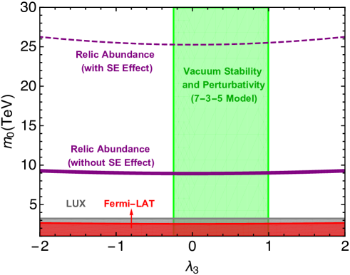
Fixing the relic abundance to its observed value ΩDMh2=0.1196±0.0031subscriptΩDMsuperscript2plus-or-minus0.11960.0031\Omega_{\mathrm{DM}}h^{2}=0.1196\pm 0.0031 [19], we can constrain the parameters m0subscript𝑚0m_{0} and λ3subscript𝜆3\lambda_{3}. In Fig. 1, the 1σ1𝜎1\sigma favored region is denoted by a purple strip in the λ3subscript𝜆3\lambda_{3}-m0subscript𝑚0m_{0} plane. In this strip, m0subscript𝑚0m_{0} increases as |λ3|subscript𝜆3|\lambda_{3}| increases. For λ3=0subscript𝜆30\lambda_{3}=0, m0subscript𝑚0m_{0} achieves its threshold mass, 8.8TeVsimilar-to-or-equalsabsent8.8TeV\simeq 8.8~{}\mathrm{TeV}. The calculation above has not included the SE effect, which can increase annihilation cross sections and hence reduce the relic abundance for fixed m0subscript𝑚0m_{0} and λ3subscript𝜆3\lambda_{3}. As suggested in Refs. [2, 4], the SE factor at the freeze-out epoch is almost a constant, and we can simply increase σeffvdelimited-⟨⟩subscript𝜎eff𝑣\langle\sigma_{\mathrm{eff}}v\rangle by a scale factor 8similar-to-or-equalsabsent8\simeq 8 to take this effect into account in the septuplet model. The dashed purple line in Fig. 1 corresponds to the observed relic abundance including the SE effect. In this case, the threshold mass is about 25 TeV.
Refer to caption
Figure 1: Regions favored by the observed DM relic abundance in the λ3subscript𝜆3\lambda_{3}-m0subscript𝑚0m_{0} plane. The purple (dashed) strip corresponds to the 1σ1𝜎1\sigma range of the relic abundance measured by the Planck experiment for the case without (with) the Sommerfeld enhancement effect. The green band is the region satisfying the vacuum stability and the perturbativity conditions in the 7-3-5 model. The grey and red regions are excluded by the LUX and Fermi-LAT results at 90% and 95% C.L., respectively.

A more accurate treatment for the DM relic abundance in real scalar MDM models can be found in Ref. [4], and gives a threshold septuplet mass of 7.9(22.4)TeV7.922.4TeV7.9~{}(22.4)~{}\textrm{TeV} without (with) the SE effect using the WMAP data. These results are about 10% smaller than our approximate results here. Nonetheless, these discrepancies would not essentially change the following analysis on the vacuum stability and the perturbativity of couplings.

We also briefly comment on the direct and indirect detection bounds on this DM candidate. At tree level, only the SM Higgs boson mediates the DM-nucleon scattering, but the rate is greatly suppressed by the heavy DM mass squared and thus is negligible as long as λ3subscript𝜆3\lambda_{3} is not very large (later we will see that this is true after taking into account vacuum stability). However, at loop level there is a contribution that is not so suppressed [1]:

σDM-N(1)=36πα24fN2mN4mW2(1mW2+1mh2)2.subscriptsuperscript𝜎1DM-𝑁36𝜋superscriptsubscript𝛼24superscriptsubscript𝑓𝑁2superscriptsubscript𝑚𝑁4superscriptsubscript𝑚𝑊2superscript1superscriptsubscript𝑚𝑊21superscriptsubscript𝑚22\sigma^{(1)}_{\text{DM-}N}=\frac{36\pi\alpha_{2}^{4}f_{N}^{2}m_{N}^{4}}{m_{W}^{2}}\left(\frac{1}{m_{W}^{2}}+\frac{1}{m_{h}^{2}}\right)^{2}. (20)

where fN0.3similar-to-or-equalssubscript𝑓𝑁0.3f_{N}\simeq 0.3 is the nucleonic form factor [20] and mN1GeVsimilar-to-or-equalssubscript𝑚𝑁1GeVm_{N}\simeq 1~{}\mathrm{GeV} is the nucleon mass. This cross section, independent of m0subscript𝑚0m_{0}, has a value of 4×1044cm2similar-to-or-equalsabsent4superscript1044superscriptcm2\simeq 4\times 10^{-44}~{}\textrm{cm}^{2}. Therefore, the 90% C.L. exclusion limit from LUX [21] can exclude the range of m03.3TeVless-than-or-similar-tosubscript𝑚03.3TeVm_{0}\lesssim 3.3~{}\mathrm{TeV}, as shown by the grey region in Fig. 1. For indirect searches, the most promising annihilation channel is the W+Wsuperscript𝑊superscript𝑊W^{+}W^{-} channel, which has a cross section 9g24/πmDM2similar-toabsent9superscriptsubscript𝑔24𝜋superscriptsubscript𝑚DM2\sim 9g_{2}^{4}/\pi m_{\rm DM}^{2} 444The ZZ/hh𝑍𝑍ZZ/hh channels produce similar gamma-ray spectra to that from the WW𝑊𝑊WW channel [22], but the cross section λ32/64πmDM2similar-to-or-equalsabsentsuperscriptsubscript𝜆3264𝜋superscriptsubscript𝑚DM2\simeq\lambda_{3}^{2}/64\pi m_{\rm DM}^{2}, depending on λ3subscript𝜆3\lambda_{3}.. The Fermi-LAT limit [23] excludes the range of m02.5TeVgreater-than-or-equivalent-tosubscript𝑚02.5TeVm_{0}\gtrsim 2.5~{}\mathrm{TeV} for |λ3|2less-than-or-similar-tosubscript𝜆32|\lambda_{3}|\lesssim 2, as shown by the red region in Fig. 1.

2.2.2 Vacum stability

The VS conditions can be obtained by means of the copositive criteria [24]. However, it is not quite straightforward to obtain these conditions in the septuplet model. The obstacle is from the quartic term 𝒬1(ΦSabΦ)2subscript𝒬1superscriptsuperscriptΦsuperscript𝑆𝑎𝑏Φ2\mathcal{Q}_{1}\equiv(\Phi^{\dagger}S^{ab}\Phi)^{2}, which, unlike the conventional term 𝒬0(ΦΦ)2subscript𝒬0superscriptsuperscriptΦΦ2\mathcal{Q}_{0}\equiv(\Phi^{\dagger}\Phi)^{2}, yields non-universal (even in sign) quartic terms for different components. To see this, we explicitly expand 𝒬1subscript𝒬1\mathcal{Q}_{1} in components as

𝒬148=subscript𝒬148absent\displaystyle\frac{\mathcal{Q}_{1}}{48}= 18(Δ(0))4+2132|Δ(1)|4+2532|Δ(3)|418superscriptsuperscriptΔ042132superscriptsuperscriptΔ142532superscriptsuperscriptΔ34\displaystyle\frac{1}{8}(\Delta^{(0)})^{4}+\frac{21}{32}|\Delta^{(1)}|^{4}+\frac{25}{32}|\Delta^{(3)}|^{4} (21)
+12|Δ(1)|2(Δ(0))2+54|Δ(2)|2(Δ(0))258|Δ(3)|2(Δ(0))212superscriptsuperscriptΔ12superscriptsuperscriptΔ0254superscriptsuperscriptΔ22superscriptsuperscriptΔ0258superscriptsuperscriptΔ32superscriptsuperscriptΔ02\displaystyle+\frac{1}{2}|\Delta^{(1)}|^{2}(\Delta^{(0)})^{2}+\frac{5}{4}|\Delta^{(2)}|^{2}(\Delta^{(0)})^{2}-\frac{5}{8}|\Delta^{(3)}|^{2}(\Delta^{(0)})^{2}
+1516|Δ(1)|2|Δ(2)|2516|Δ(1)|2|Δ(3)|2+2516|Δ(2)|2|Δ(3)|21516superscriptsuperscriptΔ12superscriptsuperscriptΔ22516superscriptsuperscriptΔ12superscriptsuperscriptΔ322516superscriptsuperscriptΔ22superscriptsuperscriptΔ32\displaystyle+\frac{15}{16}|\Delta^{(1)}|^{2}|\Delta^{(2)}|^{2}-\frac{5}{16}|\Delta^{(1)}|^{2}|\Delta^{(3)}|^{2}+\frac{25}{16}|\Delta^{(2)}|^{2}|\Delta^{(3)}|^{2}
1582(Δ(2)(Δ(1))2Δ(0)+Δ(2)(Δ(1))2Δ(0))1582superscriptΔ2superscriptsuperscriptΔ12superscriptΔ0superscriptΔ2superscriptsuperscriptΔ12superscriptΔ0\displaystyle-\frac{\sqrt{15}}{8\sqrt{2}}(\Delta^{(-2)}(\Delta^{(1)})^{2}\Delta^{(0)}+\Delta^{(2)}(\Delta^{(-1)})^{2}\Delta^{(0)})
158(Δ(3)(Δ(1))3+(Δ(1))3Δ(3))158superscriptΔ3superscriptsuperscriptΔ13superscriptsuperscriptΔ13superscriptΔ3\displaystyle-\frac{\sqrt{15}}{8}(\Delta^{(-3)}(\Delta^{(1)})^{3}+(\Delta^{(-1)})^{3}\Delta^{(3)})
+51615(Δ(3)Δ(1)(Δ(2))2+(Δ(2))2Δ(1)Δ(3))51615superscriptΔ3superscriptΔ1superscriptsuperscriptΔ22superscriptsuperscriptΔ22superscriptΔ1superscriptΔ3\displaystyle+\frac{5}{16}\sqrt{15}(\Delta^{(-3)}\Delta^{(-1)}(\Delta^{(2)})^{2}+(\Delta^{(-2)})^{2}\Delta^{(1)}\Delta^{(3)})
+1582(Δ(3)Δ(1)Δ(2)Δ(0)+Δ(2)Δ(1)Δ(3)Δ(0)).1582superscriptΔ3superscriptΔ1superscriptΔ2superscriptΔ0superscriptΔ2superscriptΔ1superscriptΔ3superscriptΔ0\displaystyle+\frac{15}{8\sqrt{2}}(\Delta^{(-3)}\Delta^{(1)}\Delta^{(2)}\Delta^{(0)}+\Delta^{(-2)}\Delta^{(-1)}\Delta^{(3)}\Delta^{(0)}).

Vacuum stability concerns the behavior of the potential as the field values go to infinity. This allows us to reduce 𝒬1subscript𝒬1\mathcal{Q}_{1}. The key observation is that the ratio 𝒬1/(48𝒬0)subscript𝒬148subscript𝒬0\mathcal{Q}_{1}/(48\mathcal{Q}_{0}) reaches its maximum 25/32253225/32 and minimum 0 when ΦΦ\Phi goes to infinity along the Δ(3)superscriptΔ3\Delta^{(3)} and Δ(2)superscriptΔ2\Delta^{(2)} directions, respectively. Therefore, we can parametrize 𝒬1/48subscript𝒬148\mathcal{Q}_{1}/48 as 25ρ𝒬0/3225𝜌subscript𝒬03225\rho\mathcal{Q}_{0}/32 with 0ρ10𝜌10\leq\rho\leq 1. Then the potential becomes

V𝑉\displaystyle V =\displaystyle= μ2HH+m2ΦΦ+λ(HH)2+λ3(HH)(ΦΦ)superscript𝜇2superscript𝐻𝐻superscript𝑚2superscriptΦΦ𝜆superscriptsuperscript𝐻𝐻2subscript𝜆3superscript𝐻𝐻superscriptΦΦ\displaystyle\mu^{2}H^{\dagger}H+m^{2}\Phi^{\dagger}\Phi+\lambda(H^{\dagger}H)^{2}+\lambda_{3}(H^{\dagger}H)(\Phi^{\dagger}\Phi) (22)
+[(λ2+λ4)+2532ρλ4](ΦΦ)2.delimited-[]subscript𝜆2subscript𝜆42532𝜌subscript𝜆4superscriptsuperscriptΦΦ2\displaystyle+\left[(\lambda_{2}+\lambda_{4})+\frac{25}{32}\rho\lambda_{4}\right](\Phi^{\dagger}\Phi)^{2}.

Now we can use the copositive criteria to get the VS conditions, which depend on the sign of λ4subscript𝜆4\lambda_{4}. For λ40subscript𝜆40\lambda_{4}\geq 0, the bottom of the potential is achieved when ρ=0𝜌0\rho=0 and the VS conditions are

{λ0,λ2+λ40,λ3+2λ(λ2+λ4)0.\displaystyle\left\{\begin{matrix}\lambda\geq 0,\\ \lambda_{2}+\lambda_{4}\geq 0,\\ \lambda_{3}+2\sqrt{\lambda(\lambda_{2}+\lambda_{4})}\geq 0.\end{matrix}\right. (23)

While for λ4<0subscript𝜆40\lambda_{4}<0 the bottom is achieved when ρ=1𝜌1\rho=1, and the VS conditions turn out to be

{λ0,λ2+5732λ40,λ3+2λ(λ2+5732λ4)0.\displaystyle\left\{\begin{matrix}\lambda\geq 0,\\ \lambda_{2}+\frac{57}{32}\lambda_{4}\geq 0,\\ \lambda_{3}+2\sqrt{\lambda\left(\lambda_{2}+\frac{57}{32}\lambda_{4}\right)}\geq 0.\end{matrix}\right. (24)

Note that λ𝜆\lambda can never be negative.

3 Confronting perturbativity

In the framework of quantum field theory, perturbativity is important to guarantee the self-consistency of perturbative calculations. The breakdown of perturbativity at some scale, known as the Landau pole scale ΛLPsubscriptΛLP\Lambda_{\mathrm{LP}}, implies that a new theory should appear hereafter. Perturbativity imposes a strong bound on models. In this section we firstly show that the minimal model suffers the Landau pole problem around 108superscript10810^{8} GeV. Then we attempt to push it up to 1014superscript101410^{14} GeV by introducing Yukawa couplings to the septuplet.

3.1 Perturbativity bound on the septuplet model

In the real scalar septuplet MDM model, there are mainly two modifications that may endanger perturbativity. One is a large positive contribution to the beta function of g2subscript𝑔2g_{2} from the 7-dimensional representation. It drives g2subscript𝑔2g_{2} towards the Landau pole more quickly. The other one is the focus of this paper, the fast increase of MDM self-couplings owing to their impressively large beta functions. Explicitly, the one-loop formulas can be calculated using the general formulas presented in Ref. [25] (or instead formulas up to two-loop are available using the code PyR@TE [26]),

βg1subscript𝛽subscript𝑔1\displaystyle\beta_{g_{1}} =\displaystyle= βg1SM,βg2=βg2SM+116π2143g23,βg3=βg3SM,βyt=βytSM,formulae-sequencesuperscriptsubscript𝛽subscript𝑔1SMsubscript𝛽subscript𝑔2superscriptsubscript𝛽subscript𝑔2SM116superscript𝜋2143superscriptsubscript𝑔23formulae-sequencesubscript𝛽subscript𝑔3superscriptsubscript𝛽subscript𝑔3SMsubscript𝛽subscript𝑦𝑡superscriptsubscript𝛽subscript𝑦𝑡SM\displaystyle\beta_{g_{1}}^{\mathrm{SM}},~{}~{}\beta_{g_{2}}=\beta_{g_{2}}^{\mathrm{SM}}+\frac{1}{16\pi^{2}}\frac{14}{3}g_{2}^{3},~{}~{}\beta_{g_{3}}=\beta_{g_{3}}^{\mathrm{SM}},~{}~{}\beta_{y_{t}}=\beta_{y_{t}}^{\mathrm{SM}}, (25)
βλsubscript𝛽𝜆\displaystyle\beta_{\lambda} =\displaystyle= βλSM+116π272λ32,βλ2=116π2[30λ22+2λ32+452λ42+51λ2λ4144g22λ2],superscriptsubscript𝛽𝜆SM116superscript𝜋272superscriptsubscript𝜆32subscript𝛽subscript𝜆2116superscript𝜋2delimited-[]30superscriptsubscript𝜆222superscriptsubscript𝜆32452superscriptsubscript𝜆4251subscript𝜆2subscript𝜆4144superscriptsubscript𝑔22subscript𝜆2\displaystyle\beta_{\lambda}^{\mathrm{SM}}+\frac{1}{16\pi^{2}}\frac{7}{2}\lambda_{3}^{2},~{}~{}\beta_{\lambda_{2}}=\frac{1}{16\pi^{2}}[30\lambda_{2}^{2}+2\lambda_{3}^{2}+\frac{45}{2}\lambda_{4}^{2}+51\lambda_{2}\lambda_{4}-144g_{2}^{2}\lambda_{2}], (26)
βλ3subscript𝛽subscript𝜆3\displaystyle\beta_{\lambda_{3}} =\displaystyle= 116π2[12λλ3+18λ2λ3+4λ32+512λ3λ4+36g24λ3(1532g22+910g126yt2)],116superscript𝜋2delimited-[]12𝜆subscript𝜆318subscript𝜆2subscript𝜆34superscriptsubscript𝜆32512subscript𝜆3subscript𝜆436superscriptsubscript𝑔24subscript𝜆31532superscriptsubscript𝑔22910superscriptsubscript𝑔126superscriptsubscript𝑦𝑡2\displaystyle\frac{1}{16\pi^{2}}\left[12\lambda\lambda_{3}+18\lambda_{2}\lambda_{3}+4\lambda_{3}^{2}+\frac{51}{2}\lambda_{3}\lambda_{4}+36g_{2}^{4}-\lambda_{3}\left(\frac{153}{2}g_{2}^{2}+\frac{9}{10}g_{1}^{2}-6y_{t}^{2}\right)\right],
βλ4subscript𝛽subscript𝜆4\displaystyle\beta_{\lambda_{4}} =\displaystyle= 116π2[288g24+2558λ42+24λ2λ4144g22λ4].116superscript𝜋2delimited-[]288superscriptsubscript𝑔242558superscriptsubscript𝜆4224subscript𝜆2subscript𝜆4144superscriptsubscript𝑔22subscript𝜆4\displaystyle\frac{1}{16\pi^{2}}\left[288g_{2}^{4}+\frac{255}{8}\lambda_{4}^{2}+24\lambda_{2}\lambda_{4}-144g_{2}^{2}\lambda_{4}\right].\qquad (28)

Our results coincide with those obtained in Ref. [17] except for the λ3λ4subscript𝜆3subscript𝜆4\lambda_{3}\lambda_{4}-term in βλ3subscript𝛽subscript𝜆3\beta_{\lambda_{3}}, which seems to be overlooked in that paper. But it does not affect perturbativity much. Additionally, we have rescaled the quartic couplings λ4subscript𝜆4\lambda_{4} by a factor 1/481481/48 and thus the numerical coefficients differ much from theirs. The beta functions in the SM are

βg1SM=116π24110g13,βg2SM=116π2(196)g23,βg3SM=116π2(7)g33,formulae-sequencesuperscriptsubscript𝛽subscript𝑔1SM116superscript𝜋24110superscriptsubscript𝑔13formulae-sequencesuperscriptsubscript𝛽subscript𝑔2SM116superscript𝜋2196superscriptsubscript𝑔23superscriptsubscript𝛽subscript𝑔3SM116superscript𝜋27superscriptsubscript𝑔33\displaystyle\beta_{g_{1}}^{\mathrm{SM}}=\frac{1}{16\pi^{2}}\frac{41}{10}g_{1}^{3},~{}~{}\beta_{g_{2}}^{\mathrm{SM}}=\frac{1}{16\pi^{2}}\left(-\frac{19}{6}\right)g_{2}^{3},~{}~{}\beta_{g_{3}}^{\mathrm{SM}}=\frac{1}{16\pi^{2}}(-7)g_{3}^{3}, (29)
βytSM=116π2yt(92yt294g221720g128g32),superscriptsubscript𝛽subscript𝑦𝑡SM116superscript𝜋2subscript𝑦𝑡92superscriptsubscript𝑦𝑡294superscriptsubscript𝑔221720superscriptsubscript𝑔128superscriptsubscript𝑔32\displaystyle\beta_{y_{t}}^{\mathrm{SM}}=\frac{1}{16\pi^{2}}y_{t}\left(\frac{9}{2}y_{t}^{2}-\frac{9}{4}g_{2}^{2}-\frac{17}{20}g_{1}^{2}-8g_{3}^{2}\right), (30)
βλSM=116π2{24λ26yt4+38[2g24+(g22+35g12)2]+λ(9g2295g12+12yt2)}.superscriptsubscript𝛽𝜆SM116superscript𝜋224superscript𝜆26superscriptsubscript𝑦𝑡438delimited-[]2superscriptsubscript𝑔24superscriptsuperscriptsubscript𝑔2235superscriptsubscript𝑔122𝜆9superscriptsubscript𝑔2295superscriptsubscript𝑔1212superscriptsubscript𝑦𝑡2\displaystyle\beta_{\lambda}^{\mathrm{SM}}=\frac{1}{16\pi^{2}}\left\{24\lambda^{2}-6y_{t}^{4}+\frac{3}{8}\left[2g_{2}^{4}+\left(g_{2}^{2}+\frac{3}{5}g_{1}^{2}\right)^{2}\right]+\lambda\left(-9g_{2}^{2}-\frac{9}{5}g_{1}^{2}+12y_{t}^{2}\right)\right\}.
(31)

From the weak scale to the septuplet threshold, couplings are evolving according to these functions.

Before heading towards the numerical study, we briefly introduce some numerical conventions. The MS¯¯MS\overline{\mathrm{MS}} values of gauge couplings at the electroweak scale are given by [27]

αs(mZ)=gs(mZ)24π=0.1184±0.0007,subscript𝛼𝑠subscript𝑚𝑍subscript𝑔𝑠superscriptsubscript𝑚𝑍24𝜋plus-or-minus0.11840.0007\displaystyle\alpha_{s}(m_{Z})=\frac{g_{s}(m_{Z})^{2}}{4\pi}=0.1184\pm 0.0007, (32)
α(mZ)=[g2(mZ)sW(mZ)]24π=1127.926,𝛼subscript𝑚𝑍superscriptdelimited-[]subscript𝑔2subscript𝑚𝑍subscript𝑠𝑊subscript𝑚𝑍24𝜋1127.926\displaystyle\alpha(m_{Z})=\frac{[g_{2}(m_{Z})s_{W}(m_{Z})]^{2}}{4\pi}=\frac{1}{127.926}, (33)
sW2=sin2θW(mZ)=0.2312.superscriptsubscript𝑠𝑊2superscript2subscript𝜃𝑊subscript𝑚𝑍0.2312\displaystyle s_{W}^{2}=\sin^{2}\theta_{W}(m_{Z})=0.2312. (34)

The measured values of ytsubscript𝑦𝑡y_{t} and λ𝜆\lambda are actually determined from the observed masses of the top quark and the Higgs boson, mtsubscript𝑚𝑡m_{t} and mhsubscript𝑚m_{h}, respectively. Therefore, we need to derive the MS¯¯MS\overline{\mathrm{MS}} values yt(mZ)subscript𝑦𝑡subscript𝑚𝑍y_{t}(m_{Z}) and λ(mZ)𝜆subscript𝑚𝑍\lambda(m_{Z}) at the electroweak scale by the matching conditions [28]

yt(μ0)=2mtv[1+δt(μ0)],λ(μ0)=mh22v2[1+δh(μ0)],formulae-sequencesubscript𝑦𝑡subscript𝜇02subscript𝑚𝑡𝑣delimited-[]1subscript𝛿𝑡subscript𝜇0𝜆subscript𝜇0superscriptsubscript𝑚22superscript𝑣2delimited-[]1subscript𝛿subscript𝜇0y_{t}(\mu_{0})=\frac{\sqrt{2}m_{t}}{v}[1+\delta_{t}(\mu_{0})],~{}~{}\lambda(\mu_{0})=\frac{m_{h}^{2}}{2v^{2}}[1+\delta_{h}(\mu_{0})], (35)

with setting μ0=mZsubscript𝜇0subscript𝑚𝑍\mu_{0}=m_{Z}. The related functions are

δt(μ0)subscript𝛿𝑡subscript𝜇0\displaystyle\delta_{t}(\mu_{0}) =\displaystyle= (4αs4π43α4π+94mt216π2v2)lnμ02mt2+ct,4subscript𝛼𝑠4𝜋43𝛼4𝜋94superscriptsubscript𝑚𝑡216superscript𝜋2superscript𝑣2superscriptsubscript𝜇02superscriptsubscript𝑚𝑡2subscript𝑐𝑡\displaystyle\left(-\frac{4\alpha_{s}}{4\pi}-\frac{4}{3}\frac{\alpha}{4\pi}+\frac{9}{4}\frac{m_{t}^{2}}{16\pi^{2}v^{2}}\right)\ln\frac{\mu_{0}^{2}}{m_{t}^{2}}+c_{t}, (36)
δh(μ0)subscript𝛿subscript𝜇0\displaystyle\delta_{h}(\mu_{0}) =\displaystyle= 2v2mh2132π2v4[h0(μ0)+mh2h1(μ0)+mh4h2(μ0)],2superscript𝑣2superscriptsubscript𝑚2132superscript𝜋2superscript𝑣4delimited-[]subscript0subscript𝜇0superscriptsubscript𝑚2subscript1subscript𝜇0superscriptsubscript𝑚4subscript2subscript𝜇0\displaystyle\frac{2v^{2}}{m_{h}^{2}}\frac{1}{32\pi^{2}v^{4}}[h_{0}(\mu_{0})+m_{h}^{2}h_{1}(\mu_{0})+m_{h}^{4}h_{2}(\mu_{0})], (37)
h0(μ0)subscript0subscript𝜇0\displaystyle h_{0}(\mu_{0}) =\displaystyle= 24mt4lnμ02mt2+6mZ4lnμ02mZ2+12mW4lnμ02mW2+c0,24superscriptsubscript𝑚𝑡4superscriptsubscript𝜇02superscriptsubscript𝑚𝑡26superscriptsubscript𝑚𝑍4superscriptsubscript𝜇02superscriptsubscript𝑚𝑍212superscriptsubscript𝑚𝑊4superscriptsubscript𝜇02superscriptsubscript𝑚𝑊2subscript𝑐0\displaystyle-24m_{t}^{4}\ln\frac{\mu_{0}^{2}}{m_{t}^{2}}+6m_{Z}^{4}\ln\frac{\mu_{0}^{2}}{m_{Z}^{2}}+12m_{W}^{4}\ln\frac{\mu_{0}^{2}}{m_{W}^{2}}+c_{0}, (38)
h1(μ0)subscript1subscript𝜇0\displaystyle h_{1}(\mu_{0}) =\displaystyle= 12mt2lnμ02mt26mZ2lnμ02mZ212mW2lnμ02mW2+c1,12superscriptsubscript𝑚𝑡2superscriptsubscript𝜇02superscriptsubscript𝑚𝑡26superscriptsubscript𝑚𝑍2superscriptsubscript𝜇02superscriptsubscript𝑚𝑍212superscriptsubscript𝑚𝑊2superscriptsubscript𝜇02superscriptsubscript𝑚𝑊2subscript𝑐1\displaystyle 12m_{t}^{2}\ln\frac{\mu_{0}^{2}}{m_{t}^{2}}-6m_{Z}^{2}\ln\frac{\mu_{0}^{2}}{m_{Z}^{2}}-12m_{W}^{2}\ln\frac{\mu_{0}^{2}}{m_{W}^{2}}+c_{1}, (39)
h2(μ0)subscript2subscript𝜇0\displaystyle h_{2}(\mu_{0}) =\displaystyle= 92lnμ02mh2+12lnμ02mZ2+lnμ02mW2+c2.92superscriptsubscript𝜇02superscriptsubscript𝑚212superscriptsubscript𝜇02superscriptsubscript𝑚𝑍2superscriptsubscript𝜇02superscriptsubscript𝑚𝑊2subscript𝑐2\displaystyle\frac{9}{2}\ln\frac{\mu_{0}^{2}}{m_{h}^{2}}+\frac{1}{2}\ln\frac{\mu_{0}^{2}}{m_{Z}^{2}}+\ln\frac{\mu_{0}^{2}}{m_{W}^{2}}+c_{2}. (40)

The constants c0subscript𝑐0c_{0}, c1subscript𝑐1c_{1}, and c2subscript𝑐2c_{2} are independent of the scale μ0subscript𝜇0\mu_{0}, and their contributions to δhsubscript𝛿\delta_{h} are less than 0.02. The constant ctsubscript𝑐𝑡c_{t} lies in the range of 0.052ct0.0420.052subscript𝑐𝑡0.042-0.052\leq c_{t}\leq-0.042. Thus we neglect c0subscript𝑐0c_{0}, c1subscript𝑐1c_{1} and c2subscript𝑐2c_{2} and take ct=0.052subscript𝑐𝑡0.052c_{t}=-0.052 in the calculation. Choosing other values for ctsubscript𝑐𝑡c_{t} would not essentially change our results.

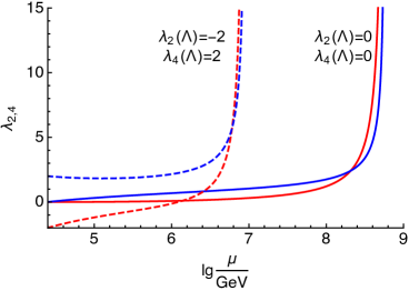
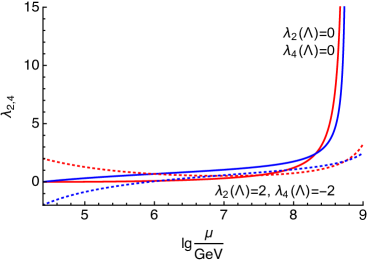
It is illustrative to make some analysis of the RGEs (25)–(28). An analytical solution is impossible, despite an approximate solution treating g2subscript𝑔2g_{2} as constant during running [17] 555The authors in Ref. [17] gave an estimation of the Landau pole as ΛLP=1.0×10⁶(m100GeV)1.13subscriptΛLP1.0superscript106superscript𝑚100GeV1.13\Lambda_{\rm LP}=1.0\times 10^{6}\left(\frac{m}{100~{}\textrm{GeV}}\right)^{1.13}.. Even if the initial values of λ2subscript𝜆2\lambda_{2} and λ4subscript𝜆4\lambda_{4} are both zero, their Landau poles appear not very far from the septuplet threshold. The presence of the λ4subscript𝜆4\lambda_{4}-term is crucial. The large positive contributions to βλ4subscript𝛽subscript𝜆4\beta_{\lambda_{4}} from the g24superscriptsubscript𝑔24g_{2}^{4}- and λ42superscriptsubscript𝜆42\lambda_{4}^{2}-terms drive λ4subscript𝜆4\lambda_{4} increasing quickly. Then the terms involving λ4subscript𝜆4\lambda_{4} in βλ2subscript𝛽subscript𝜆2\beta_{\lambda_{2}} (with large positive coefficients) push λ2subscript𝜆2\lambda_{2} towards the Landau pole. As a matter of fact, λ2subscript𝜆2\lambda_{2} hits the Landau pole first. Given the septuplet MDM threshold Λ=8.8Λ8.8\Lambda=8.8 TeV or 25 TeV and initial values of λ2(Λ)=λ4(Λ)=0subscript𝜆2Λsubscript𝜆4Λ0\lambda_{2}(\Lambda)=\lambda_{4}(\Lambda)=0, we have ΛLP108109similar-tosubscriptΛLPsuperscript108superscript109\Lambda_{\mathrm{LP}}\sim 10^{8}-10^{9} GeV. Here and henceforth, we set the septulet threshold ΛΛ\Lambda to be 252525 TeV, and the evolution of λ2subscript𝜆2\lambda_{2} and λ4subscript𝜆4\lambda_{4} are indicated by the solid lines in Fig. 2. This is consistent with the result in Ref. [17]. If the VS conditions were not imposed, it would be able to obtain a slightly higher ΛLP1010similar-tosubscriptΛLPsuperscript1010\Lambda_{\rm LP}\sim 10^{10} GeV by arranging a cancellation between the λ4λ2subscript𝜆4subscript𝜆2\lambda_{4}\lambda_{2}-term and λ22superscriptsubscript𝜆22\lambda_{2}^{2}-term in βλ2subscript𝛽subscript𝜆2\beta_{\lambda_{2}}. For instance, This can be achieved if we set λ2(Λ)=2subscript𝜆2Λ2\lambda_{2}(\Lambda)=2 and λ4(Λ)=2subscript𝜆4Λ2\lambda_{4}(\Lambda)=-2, as demonstrated in the left panel of Fig. 2. On the other hand, if λ2(Λ)<0subscript𝜆2Λ0\lambda_{2}(\Lambda)<0 and λ4(Λ)>0subscript𝜆4Λ0\lambda_{4}(\Lambda)>0, the situation would be even worse, as shown in the right panel of Fig. 2.
Refer to caption
Refer to caption
Figure 2: The evolution of λ2subscript𝜆2\lambda_{2} (red lines) and λ4subscript𝜆4\lambda_{4} (blue lines) in the septuplet MDM model.

3.2 Push up the Landau pole scale in the 7-3-5 model

It is potential to push up the LP scale by introducing Yukawa couplings to the septuplet. This is inspired by the beta function structure of the Higgs self-coupling λ𝜆\lambda. It receives a large negative contribution from the top quark Yukawa coupling, which incurs the metastable problem of the electroweak vacuum at high scales. We will firstly present the 7-3-5 model, which is an extension to the septuplet model, and then analyze its implication to the Landau pole problem.

3.2.1 The 7-3-5 model

In order to construct Yukawa couplings to the septuplet, extra fermions should be introduced. Three minimal ways are available: (1,0)(7,0)direct-sum1070(1,0)\oplus(7,0), (3,0)(5,0)direct-sum3050(3,0)\oplus(5,0) and (4,0)(4,0)direct-sum4040(4,0)\oplus(4,0). The first and second options have potential of explaining the tiny neutrino masses via the type-I and type-III seesaw mechanisms666There are some models with quintuplet fermion and septuplet scalar for generating neutrino masses at loop level [29, 30, 31]., respectively. However, we find that the first option is not as good as the second one due to a fairly large contribution to βg2subscript𝛽subscript𝑔2\beta_{g_{2}} from the fermionic septuplet. On the other hand, in the last option, if the two (4,0)40(4,0) fermions belong to the same chiral field (namely being Majorana fermions), it would lead to the problem of Witten global anomaly [32, 33]. Even worse, the Majorana mass term violates the accidental Z2subscript𝑍2Z_{2} symmetry of the septuplet and thus leads to the septuplet MDM radiatively decay into a pair of gauge bosons. A (4,0)40(4,0) Dirac fermion avoids the Witten global anomaly, but it similarly endangers the stability of MDM at loop level. Therefore, in this work we concentrate on the (3,0)(5,0)direct-sum3050(3,0)\oplus(5,0) case, and the resulting model is dubbed as the 7-3-5 model.

In order to write down the Yukawa interaction terms, it is more convenient to use the tensor notation rather than the vector notation adopted above. More details about the tensor notation can be found in Ref. [29]. The dictionary from the latter to the former notation reads

Φ=12(Δ(3)Δ(2)Δ(1)Δ(0)Δ(1)Δ(2)Δ(3))=12(Φ1111116Φ11111215Φ11112220Φ11122215Φ1122226Φ122222Φ222222),Φ12matrixsuperscriptΔ3superscriptΔ2superscriptΔ1superscriptΔ0superscriptΔ1superscriptΔ2superscriptΔ312matrixsubscriptΦ1111116subscriptΦ11111215subscriptΦ11112220subscriptΦ11122215subscriptΦ1122226subscriptΦ122222subscriptΦ222222\displaystyle\Phi=\frac{1}{\sqrt{2}}\begin{pmatrix}\Delta^{(3)}\\ \Delta^{(2)}\\ \Delta^{(1)}\\ \Delta^{(0)}\\ \Delta^{(-1)}\\ \Delta^{(-2)}\\ \Delta^{(-3)}\end{pmatrix}=\frac{1}{\sqrt{2}}\begin{pmatrix}\Phi_{111111}\\ \sqrt{6}\Phi_{111112}\\ \sqrt{15}\Phi_{111122}\\ \sqrt{20}\Phi_{111222}\\ -\sqrt{15}\Phi_{112222}\\ \sqrt{6}\Phi_{122222}\\ -\Phi_{222222}\end{pmatrix}, (41)
ΨL=(Ψ+2,LΨ+1,LΨ0,LΨ1,LΨ2,L)=(Ψ1111,L2Ψ1112,L6Ψ1122,L2Φ1222,LΦ2222,L),ΣR=(Σ+1,RΣ0,RΣ1,R)=(Σ11,R2Σ12,RΣ22,R).formulae-sequencesubscriptΨ𝐿matrixsubscriptΨ2𝐿subscriptΨ1𝐿subscriptΨ0𝐿subscriptΨ1𝐿subscriptΨ2𝐿matrixsubscriptΨ1111𝐿2subscriptΨ1112𝐿6subscriptΨ1122𝐿2subscriptΦ1222𝐿subscriptΦ2222𝐿subscriptΣ𝑅matrixsubscriptΣ1𝑅subscriptΣ0𝑅subscriptΣ1𝑅matrixsubscriptΣ11𝑅2subscriptΣ12𝑅subscriptΣ22𝑅\displaystyle\Psi_{L}=\begin{pmatrix}\Psi_{+2,L}\\ \Psi_{+1,L}\\ \Psi_{0,L}\\ \Psi_{-1,L}\\ \Psi_{-2,L}\end{pmatrix}=\begin{pmatrix}\Psi_{1111,L}\\ 2\Psi_{1112,L}\\ \sqrt{6}\Psi_{1122,L}\\ -2\Phi_{1222,L}\\ \Phi_{2222,L}\end{pmatrix},~{}~{}\Sigma_{R}=\begin{pmatrix}\Sigma_{+1,R}\\ \Sigma_{0,R}\\ \Sigma_{-1,R}\end{pmatrix}=\begin{pmatrix}\Sigma_{11,R}\\ \sqrt{2}\Sigma_{12,R}\\ -\Sigma_{22,R}\end{pmatrix}. (42)

Here we have assigned the left and right chiralities to the quintuplet and triplet, respectively. At renormalizable level the most generic Yukawa interactions can be written down as

yuk=subscriptyukabsent\displaystyle\mathcal{L}_{\mathrm{yuk}}= 15yΦijklmnΨLijkl¯ΣR,mnεmmεnn15𝑦subscriptΦ𝑖𝑗𝑘𝑙𝑚𝑛¯superscriptsubscriptΨ𝐿𝑖𝑗𝑘𝑙subscriptΣ𝑅superscript𝑚superscript𝑛superscript𝜀𝑚superscript𝑚superscript𝜀𝑛superscript𝑛\displaystyle-\sqrt{15}y\Phi_{ijklmn}\overline{\Psi_{L}^{ijkl}}\Sigma_{R,m^{\prime}n^{\prime}}\varepsilon^{mm^{\prime}}\varepsilon^{nn^{\prime}} (43)
(yΣ)abla,Li¯(Σb,R)ijHkεjk+h.c.,formulae-sequencesubscriptsubscript𝑦Σ𝑎𝑏¯superscriptsubscript𝑙𝑎𝐿𝑖subscriptsubscriptΣ𝑏𝑅𝑖𝑗subscript𝐻𝑘superscript𝜀𝑗𝑘hc\displaystyle-(y_{\Sigma})_{ab}\overline{l_{a,L}^{i}}(\Sigma_{b,R})_{ij}H_{k}\varepsilon^{jk}+\mathrm{h.c.}, (44)

where i,j,k,l,m,n=1,2formulae-sequence𝑖𝑗𝑘𝑙𝑚𝑛12i,j,k,l,m,n=1,2 are SU(2)L𝑆𝑈subscript2𝐿SU(2)_{L} tensor indices and symmetric for ΦΦ\Phi, ΨΨ\Psi, and ΣΣ\Sigma. a𝑎a and b𝑏b are family indices and for the sake of realistic neutrino mixing at least two triplets are required. Terms in the second line, along with Majorana mass terms for the fermions, constitute the type-III seesaw mechanism. The Yukawa couplings yΣsubscript𝑦Σy_{\Sigma} are irrelevantly small. Note that the 7-dimensional representation from the decomposition 5×5=1S+3A+5S+7A+9S55subscript1𝑆subscript3𝐴subscript5𝑆subscript7𝐴subscript9𝑆5\times 5=1_{S}+3_{A}+5_{S}+7_{A}+9_{S} is antisymmetric, thus the coupling ΦΨΨΦΨΨ\Phi\Psi\Psi vanishes. In the vector notation, Eq. (43) gives the Yukawa couplings of the septuplet as

yuksubscriptyuk\displaystyle\mathcal{L}_{\mathrm{yuk}} =\displaystyle= y2{[Δ(0)3Ψ1¯Σ1+Δ(1)(6Ψ0¯Σ+122Ψ1¯Σ0+Ψ2¯Σ1)\displaystyle\frac{y}{\sqrt{2}}\{[\Delta^{(0)}\sqrt{3}\overline{\Psi_{-1}}\Sigma_{-1}+\Delta^{(-1)}(-\sqrt{6}\overline{\Psi_{0}}\Sigma_{+1}-2\sqrt{2}\overline{\Psi_{-1}}\Sigma_{0}+\overline{\Psi_{-2}}\Sigma_{-1}) (45)
+Δ(2)(10Ψ1¯Σ+15Ψ2¯Σ0)15Δ(3)Ψ2¯Σ+1+h.c.]\displaystyle\qquad~{}+\Delta^{(-2)}(-\sqrt{10}\overline{\Psi_{-1}}\Sigma_{+1}-\sqrt{5}\overline{\Psi_{-2}}\Sigma_{0})-\sqrt{15}\Delta^{(-3)}\overline{\Psi_{-2}}\Sigma_{+1}+\mathrm{h.c.}]
3Δ(0)Ψ0¯Σ0}.\displaystyle\qquad-3\Delta^{(0)}\overline{\Psi_{0}}\Sigma_{0}\}.

Where ΨQ=ΨQ,L+(Ψ+Q,L)csubscriptΨ𝑄subscriptΨ𝑄𝐿superscriptsubscriptΨ𝑄𝐿𝑐\Psi_{-Q}=\Psi_{-Q,L}+(\Psi_{+Q,L})^{c} and ΣQ=ΣQ,L+(Σ+Q,L)csubscriptΣ𝑄subscriptΣ𝑄𝐿superscriptsubscriptΣ𝑄𝐿𝑐\Sigma_{-Q}=\Sigma_{-Q,L}+(\Sigma_{+Q,L})^{c}. The gauge couplings of the fermions are

gaugesubscriptgauge\displaystyle\mathcal{L}_{\mathrm{gauge}} =\displaystyle= g2[(3Ψ0¯γμΨ1+2Ψ1¯γμΨ2)Wμ++Σ0¯γμΣ1Wμ++h.c.]\displaystyle g_{2}[(\sqrt{3}\overline{\Psi_{0}}\gamma^{\mu}\Psi_{-1}+\sqrt{2}\overline{\Psi_{-1}}\gamma^{\mu}\Psi_{-2})W^{+}_{\mu}+\overline{\Sigma_{0}}\gamma^{\mu}\Sigma_{-1}W^{+}_{\mu}+\mathrm{h.c.}] (46)
+g2(Q=12QΨQ¯γμΨQ+Σ+1¯γμΣ+1)Wμ3.subscript𝑔2superscriptsubscript𝑄12𝑄¯subscriptΨ𝑄superscript𝛾𝜇subscriptΨ𝑄¯subscriptΣ1superscript𝛾𝜇subscriptΣ1subscriptsuperscript𝑊3𝜇\displaystyle+g_{2}(\sum_{Q=1}^{2}Q\overline{\Psi_{Q}}\gamma^{\mu}\Psi_{Q}+\overline{\Sigma_{+1}}\gamma^{\mu}\Sigma_{+1})W^{3}_{\mu}.

The presence of the quintuplet and triplet further modifies the one-loop beta functions with the following extra terms:

δβg2𝛿subscript𝛽subscript𝑔2\displaystyle\delta\beta_{g_{2}} =\displaystyle= 8g2316π2,8superscriptsubscript𝑔2316superscript𝜋2\displaystyle\frac{8g_{2}^{3}}{16\pi^{2}}, (47)
δβλ2𝛿subscript𝛽subscript𝜆2\displaystyle\delta\beta_{\lambda_{2}} =\displaystyle= 116π2(54y4+40y2λ2),116superscript𝜋254superscript𝑦440superscript𝑦2subscript𝜆2\displaystyle\frac{1}{16\pi^{2}}(-54y^{4}+40y^{2}\lambda_{2}), (48)
δβλ3𝛿subscript𝛽subscript𝜆3\displaystyle\delta\beta_{\lambda_{3}} =\displaystyle= 20y2λ316π2,20superscript𝑦2subscript𝜆316superscript𝜋2\displaystyle\frac{20y^{2}\lambda_{3}}{16\pi^{2}}, (49)
δβλ4𝛿subscript𝛽subscript𝜆4\displaystyle\delta\beta_{\lambda_{4}} =\displaystyle= 116π2(96y4+40y2λ4),116superscript𝜋296superscript𝑦440superscript𝑦2subscript𝜆4\displaystyle\frac{1}{16\pi^{2}}(-96y^{4}+40y^{2}\lambda_{4}), (50)
βysubscript𝛽𝑦\displaystyle\beta_{y} =\displaystyle= y16π2(25y224g22).𝑦16superscript𝜋225superscript𝑦224superscriptsubscript𝑔22\displaystyle\frac{y}{16\pi^{2}}(25y^{2}-24g_{2}^{2}). (51)

As expected, the Yukawa coupling y𝑦y has negative contributions to βλ2subscript𝛽subscript𝜆2\beta_{\lambda_{2}} and βλ4subscript𝛽subscript𝜆4\beta_{\lambda_{4}}. Below we study how the LP scale can be substantially pushed up by this coupling.

3.2.2 How high can the Landau pole scale be?

Now we have two free parameters at hand. One is y𝑦y; the other one is M35subscript𝑀35M_{35}, the threshold above which the 7-3-5 Yukawa coupling becomes active. The mass scales of the quintuplet and triplet are set to be equal to M35subscript𝑀35M_{35} 777In practice, M35subscript𝑀35M_{35} can be identified as the heavier one. But the situation is actually worse since the lighter fermion just induces increase in g2subscript𝑔2g_{2} from its mass to M35subscript𝑀35M_{35}.. In order to push up ΛLPsubscriptΛLP\Lambda_{\rm LP} as high as possible, we find that M35subscript𝑀35M_{35} should not be far above the MDM mass scale, and moreover the initial value of y(M35)𝑦subscript𝑀35y(M_{35}) should be fine-tuned. Thereby, the 7-3-5 model does not provide a quite satisfactory alleviation to the Landau pole problem.

First of all, the Landau pole of g2subscript𝑔2g_{2} is of concern. As shown in Eq. (47), the beta function of g2subscript𝑔2g_{2} receives large positive contributions from the quintuplet and triplet. Consequently, a low M35subscript𝑀35M_{35} would drive g2subscript𝑔2g_{2} to the Landau pole quickly 888To maximize the Landau pole scale of g2subscript𝑔2g_{2}, we assume a hierarchy between different triplet generations and only the lightest one is active at the low energy scales we concern.. The explicit solution is

α21(μ)=α21(mZ)b2SM2πlnΛmZb2sep2πlnM35Λb2tot2πlnμM35,superscriptsubscript𝛼21𝜇superscriptsubscript𝛼21subscript𝑚𝑍superscriptsubscript𝑏2SM2𝜋Λsubscript𝑚𝑍superscriptsubscript𝑏2sep2𝜋subscript𝑀35Λsuperscriptsubscript𝑏2tot2𝜋𝜇subscript𝑀35\displaystyle\alpha_{2}^{-1}(\mu)=\alpha_{2}^{-1}(m_{Z})-\frac{b_{2}^{\mathrm{SM}}}{2\pi}\ln\frac{\Lambda}{m_{Z}}-\frac{b_{2}^{\mathrm{sep}}}{2\pi}\ln\frac{M_{35}}{\Lambda}-\frac{b_{2}^{\mathrm{tot}}}{2\pi}\ln\frac{\mu}{M_{35}}, (52)

where b2SM=19/6superscriptsubscript𝑏2SM196b_{2}^{\mathrm{SM}}=-19/6, b2sep=3/2superscriptsubscript𝑏2sep32b_{2}^{\mathrm{sep}}=3/2, and b2tot=19/2superscriptsubscript𝑏2tot192b_{2}^{\mathrm{tot}}=19/2. From it one can determine the Landau pole scale of g2subscript𝑔2g_{2}:

ΛLP(g2)=M35(ΛM35)b2sep/b2totexp[2πb2totα21(Λ)].subscriptsuperscriptΛsubscript𝑔2LPsubscript𝑀35superscriptΛsubscript𝑀35superscriptsubscript𝑏2sepsuperscriptsubscript𝑏2tot2𝜋superscriptsubscript𝑏2totsuperscriptsubscript𝛼21Λ\displaystyle\Lambda^{(g_{2})}_{\rm LP}=M_{35}\left(\frac{\Lambda}{M_{35}}\right)^{b_{2}^{\mathrm{sep}}/b_{2}^{\mathrm{tot}}}\exp\left[\frac{2\pi}{b_{2}^{\mathrm{tot}}}\alpha_{2}^{-1}(\Lambda)\right]. (53)

For example, if M35=105subscript𝑀35superscript105M_{35}=10^{5} GeV, we have ΛLP(g2)=1.54×10¹⁴subscriptsuperscriptΛsubscript𝑔2LP1.54superscript1014\Lambda^{(g_{2})}_{\rm LP}=1.54\times 10^{14} GeV, far below the Planck scale. Note that typically the non-perturbative scale is only slightly lower than ΛLPsubscriptΛLP\Lambda_{\rm LP}, so we do not distinguish them in this paper.

One cannot rely on increasing M35subscript𝑀35M_{35} to lift ΛLP(g2)subscriptsuperscriptΛsubscript𝑔2LP\Lambda^{(g_{2})}_{\rm LP}. As our purpose is to push up the Landau pole scales of λ2subscript𝜆2\lambda_{2} and λ4subscript𝜆4\lambda_{4}, M35subscript𝑀35M_{35} is forced to be not far from the septuplet threshold ΛΛ\Lambda. Otherwise, λ2subscript𝜆2\lambda_{2}, perhaps as well as λ4subscript𝜆4\lambda_{4}, would quickly evolve to a sufficiently large value such that y(M35)1much-greater-than𝑦subscript𝑀351y(M_{35})\gg 1 is needed to slow down the running of λ2subscript𝜆2\lambda_{2} and λ4subscript𝜆4\lambda_{4}. Moreover, y𝑦y itself grows very fast and eventually diverges at ΛLP(y)subscriptsuperscriptΛ𝑦LP\Lambda^{(y)}_{\rm LP}, which could be much lower than ΛLP(g2)subscriptsuperscriptΛsubscript𝑔2LP\Lambda^{(g_{2})}_{\rm LP}. We can see this from the explicit expression of y(t)𝑦𝑡y(t), where tln(μ/M35)𝑡𝜇subscript𝑀35t\equiv\ln(\mu/M_{35}) denotes the logarithm of the energy scale. In practice, RGE (51) can be analytically solved:

y2(t)=(24+b2)g22(0)F0[g2(t)/g2(0)]48/b2+25[g2(t)/g2(0)]2,superscript𝑦2𝑡24subscript𝑏2subscriptsuperscript𝑔220subscript𝐹0superscriptdelimited-[]subscript𝑔2𝑡subscript𝑔2048subscript𝑏225superscriptdelimited-[]subscript𝑔2𝑡subscript𝑔202\displaystyle y^{2}(t)=\frac{(24+b_{2})g^{2}_{2}(0)}{F_{0}[g_{2}(t)/g_{2}(0)]^{48/b_{2}}+25[g_{2}(t)/g_{2}(0)]^{-2}}, (54)

with F0(24+b2)g22(0)/y2(0)25subscript𝐹024subscript𝑏2subscriptsuperscript𝑔220superscript𝑦2025F_{0}\equiv(24+b_{2})g^{2}_{2}(0)/y^{2}(0)-25 and b2=b2tot=19/2subscript𝑏2superscriptsubscript𝑏2tot192b_{2}=b_{2}^{\mathrm{tot}}=19/2.

As long as we have a large y(0)𝑦0y(0) such that F0<0subscript𝐹00F_{0}<0, y(t)𝑦𝑡y(t) will meet the Landau pole as g2(t)subscript𝑔2𝑡g_{2}(t) evolves to the value

g22(tLP(y))g22(0)(25|F0|)b2/(24+b2)=similar-to-or-equalssuperscriptsubscript𝑔22superscriptsubscript𝑡LP𝑦subscriptsuperscript𝑔220superscript25subscript𝐹0subscript𝑏224subscript𝑏2absent\displaystyle g_{2}^{2}(t_{\mathrm{LP}}^{(y)})\simeq g^{2}_{2}(0)\left(\frac{25}{|F_{0}|}\right)^{b_{2}/(24+b_{2})}= g22(0)[1(24+b2)g22(0)25y2(0)]b2/(24+b2).subscriptsuperscript𝑔220superscriptdelimited-[]124subscript𝑏2subscriptsuperscript𝑔22025superscript𝑦20subscript𝑏224subscript𝑏2\displaystyle g^{2}_{2}(0)\left[1-\frac{(24+b_{2})g^{2}_{2}(0)}{25y^{2}(0)}\right]^{-b_{2}/(24+b_{2})}. (55)

Based on this equation, it is straightforward to derive an expression for ΛLP(y)subscriptsuperscriptΛ𝑦LP\Lambda^{(y)}_{\rm LP}:

ΛLP(y)=ΛLP(g2)exp[8π2b2g22(0)(F025)b2/(24+b2)].superscriptsubscriptΛLP𝑦superscriptsubscriptΛLPsubscript𝑔28superscript𝜋2subscript𝑏2superscriptsubscript𝑔220superscriptsubscript𝐹025subscript𝑏224subscript𝑏2\displaystyle\Lambda_{\rm LP}^{(y)}=\frac{\Lambda_{\rm LP}^{(g_{2})}}{\exp\left[\dfrac{8\pi^{2}}{b_{2}g_{2}^{2}(0)}\left(\dfrac{-F_{0}}{25}\right)^{b_{2}/(24+b_{2})}\right]}. (56)

Critical values that lead to F0=0subscript𝐹00F_{0}=0 and ΛLP(y)=ΛLP(g2)superscriptsubscriptΛLP𝑦superscriptsubscriptΛLPsubscript𝑔2\Lambda_{\mathrm{LP}}^{(y)}=\Lambda_{\mathrm{LP}}^{(g_{2})} are ±ycplus-or-minussubscript𝑦𝑐\pm y_{c}, where

yc(24+b225)1/2g2(0).subscript𝑦𝑐superscript24subscript𝑏22512subscript𝑔20\displaystyle y_{c}\equiv\left(\frac{24+b_{2}}{25}\right)^{1/2}g_{2}(0). (57)

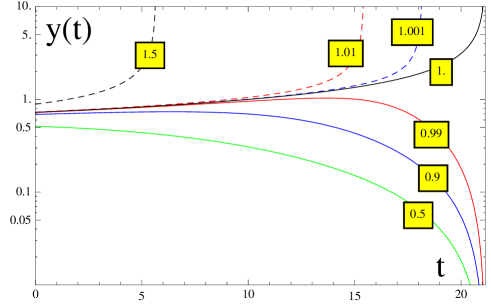
Thus F0=25[yc2/y2(0)1]subscript𝐹025delimited-[]superscriptsubscript𝑦𝑐2superscript𝑦201F_{0}=25[y_{c}^{2}/y^{2}(0)-1]. Since ΛLP(y)superscriptsubscriptΛLP𝑦\Lambda_{\rm LP}^{(y)} is exponentially suppressed compared to ΛLP(g2)superscriptsubscriptΛLPsubscript𝑔2\Lambda_{\rm LP}^{(g_{2})}, a small derivation of F0subscript𝐹0F_{0} from zero will lead to a dramatically smaller ΛLP(y)superscriptsubscriptΛLP𝑦\Lambda_{\rm LP}^{(y)}, as shown in Fig. 3, where the labels on the lines are values of y(0)𝑦0y(0) in unit of ycsubscript𝑦𝑐y_{c} and y(0)>yc𝑦0subscript𝑦𝑐y(0)>y_{c} corresponds to F0<0subscript𝐹00F_{0}<0. In other words, in order to retain a high ΛLP(y)superscriptsubscriptΛLP𝑦\Lambda_{\rm LP}^{(y)}, y(0)𝑦0y(0) must be extremely close to ±ycplus-or-minussubscript𝑦𝑐\pm y_{c}. This raises a fine-tuning problem.

Unfortunately, this kind of fine-tuning is robust in any case. In the case of F0>0subscript𝐹00F_{0}>0, y(t)𝑦𝑡y(t) no longer has a Landau pole but instead become asymptotic free as g2(t)subscript𝑔2𝑡g_{2}(t) approaches its Landau pole. Due to the large power 48/b25.148subscript𝑏25.148/b_{2}\approx 5.1, y(t)𝑦𝑡y(t) will quickly run to zero once the first term of the denominator in Eq. (54) dominates. We demonstrate this behavior for several y(0)𝑦0y(0) values in Fig. 3, where y(0)<yc𝑦0subscript𝑦𝑐y(0)<y_{c} corresponds to F0>0subscript𝐹00F_{0}>0. One can clearly see that y(0)𝑦0y(0) must be also sufficiently close to the critical value ycsubscript𝑦𝑐y_{c}, otherwise the Yukawa effect becomes negligible soon and the LP scales of λ2subscript𝜆2\lambda_{2} and λ4subscript𝜆4\lambda_{4} cannot be pushed up. Therefore, this case is not supposed to be better than the previous case. But it has an advantage that λ2subscript𝜆2\lambda_{2} and λ4subscript𝜆4\lambda_{4} are positive near their Landau poles. By contrast, in the F0<0subscript𝐹00F_{0}<0 case they run to large negative values near the Landau pole of y(t)𝑦𝑡y(t). We can see these features in Fig. 4. We leave an analytical understanding of the Landau poles of λ2subscript𝜆2\lambda_{2} and λ4subscript𝜆4\lambda_{4} in the next subsection.

Refer to caption
Figure 3: Running of y(t)𝑦𝑡y(t) for different choices of y(0)𝑦0y(0), which is the labels on the lines in unit of ycsubscript𝑦𝑐y_{c}. The LP scale of g2subscript𝑔2g_{2} is at the maximum of the t𝑡t-axis. We have chosen M35=105.5subscript𝑀35superscript105.5M_{35}=10^{5.5} GeV, but the curves are not sensitive to this value.

From this analysis we can learn how to choose values of M35subscript𝑀35M_{35} that can lead to the highest LP scales. It should be chosen to guarantee a negative βλ2(0)𝒪(0.01)similar-tosubscript𝛽subscript𝜆20𝒪0.01\beta_{\lambda_{2}}(0)\sim-\mathcal{O}(0.01) such that the most intractable coupling λ2subscript𝜆2\lambda_{2} is tamed. Bear in mind that since y(0)𝑦0y(0) has been almost fixed around 0.7 by the condition F00subscript𝐹00F_{0}\approx 0, there is a strong upper bound on M35subscript𝑀35M_{35}. In terms of our numerical investigation, the highest M35subscript𝑀35M_{35} is larger than the septuplet threshold ΛΛ\Lambda by about (typically slightly less than) 2 orders of magnitude. For instance, for mDM=22subscript𝑚DM22m_{\rm DM}=22 TeV, it is found that M35105.7subscript𝑀35superscript105.7M_{35}\approx 10^{5.7} GeV is required and the resulting maximal Landau pole scale is ΛLP1013subscriptΛLPsuperscript1013\Lambda_{\rm LP}\approx 10^{13} GeV if we tolerate y(0)=1.001yc𝑦01.001subscript𝑦𝑐y(0)=1.001y_{c}; If we only tolerate y(0)=1.01yc𝑦01.01subscript𝑦𝑐y(0)=1.01y_{c}, the maximal Landau pole is ΛLP1012subscriptΛLPsuperscript1012\Lambda_{\rm LP}\approx 10^{12} GeV with M35106.1subscript𝑀35superscript106.1M_{35}\approx 10^{6.1} GeV. We show the running in these two cases in Fig 4. For comparison, we also plot two cases with F0>0subscript𝐹00F_{0}>0: y(0)=0.99yc𝑦00.99subscript𝑦𝑐y(0)=0.99y_{c} with M35=105.5subscript𝑀35superscript105.5M_{35}=10^{5.5} GeV and ΛLP1.7×1011subscriptΛLP1.7superscript1011\Lambda_{\rm LP}\approx 1.7\times 10^{11} GeV; y(0)=0.999yc𝑦00.999subscript𝑦𝑐y(0)=0.999y_{c} with M35=105.6subscript𝑀35superscript105.6M_{35}=10^{5.6} GeV and ΛLP9.6×1011subscriptΛLP9.6superscript1011\Lambda_{\rm LP}\approx 9.6\times 10^{11} GeV.

Refer to caption
Refer to caption
Figure 4: RGE running of couplings in four cases. Top left: y(0)=1.001yc𝑦01.001subscript𝑦𝑐y(0)=1.001y_{c} with M35=105.7subscript𝑀35superscript105.7M_{35}=10^{5.7} GeV; Top right: y(0)=1.01yc𝑦01.01subscript𝑦𝑐y(0)=1.01y_{c} with M35=106.1subscript𝑀35superscript106.1M_{35}=10^{6.1} GeV; Bottom left: y(0)=0.999yc𝑦00.999subscript𝑦𝑐y(0)=0.999y_{c} with M35=105.6subscript𝑀35superscript105.6M_{35}=10^{5.6} GeV; Bottom right: y(0)=0.99yc𝑦00.99subscript𝑦𝑐y(0)=0.99y_{c} with M35=105.5subscript𝑀35superscript105.5M_{35}=10^{5.5} GeV.

3.2.3 Constraints from perturbativity and VS in the F0=0subscript𝐹00F_{0}=0 case

As a demonstration of the impacts of perturbativity and as well VS on the model, here we assume the ideal limit for F0subscript𝐹0F_{0}, i.e., it is exactly zero and then one can obtain the highest LP scale. For the given septuplet MDM mass 25 TeV, it means that we have to fine-tune the initial y(0)=0.7286422𝑦00.7286422y(0)=0.7286422.

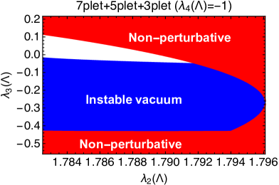
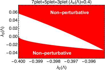
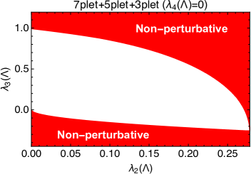
We survey 3 slices of the parameter space corresponding to λ4(Λ)=0.4subscript𝜆4Λ0.4\lambda_{4}(\Lambda)=0.4, 00, 11-1 as input, and evolve the couplings to a cutoff scale of 1014superscript101410^{14} GeV, just a little bit below the highest LP scale, and then impose the VS and perturbativity conditions to give constraints. Here the perturbativity conditions mean that the absolute value of any coupling cannot exceed 4π4𝜋4\pi. We assume M35=105.5subscript𝑀35superscript105.5M_{35}=10^{5.5} GeV and the results are shown in Fig. 5, where the blue (red) regions are excluded by the VS (perturbativity) conditions, while the white regions can fulfill both the conditions. These plots have the following features.
Refer to caption
Refer to caption
Refer to caption
Figure 5: Regions excluded by the VS (blue) and perturbativity (red) conditions in the λ2(Λ)subscript𝜆2Λ\lambda_{2}(\Lambda)-λ3(Λ)subscript𝜆3Λ\lambda_{3}(\Lambda) plane for the 7-3-5 model. The top-left (top-right) panel corresponds to λ4(Λ)=0.4(0)subscript𝜆4Λ0.40\lambda_{4}(\Lambda)=0.4~{}(0), while the bottom panel corresponds to λ4(Λ)=1subscript𝜆4Λ1\lambda_{4}(\Lambda)=-1.
  • When λ4(Λ)=0.4subscript𝜆4Λ0.4\lambda_{4}(\Lambda)=0.4, the acceptable range of λ3(Λ)subscript𝜆3Λ\lambda_{3}(\Lambda) that fulfill the two conditions is 0.034λ3(Λ)0.057less-than-or-similar-to0.034subscript𝜆3Λless-than-or-similar-to0.057-0.034\lesssim\lambda_{3}(\Lambda)\lesssim 0.057. On the other hand, λ2(Λ)subscript𝜆2Λ\lambda_{2}(\Lambda) is bounded as 0.4λ2(Λ)0.3950.4subscript𝜆2Λless-than-or-similar-to0.395-0.4\leq\lambda_{2}(\Lambda)\lesssim-0.395, which is very narrow. 0.40.40.4 is almost the upper bound on λ4(Λ)subscript𝜆4Λ\lambda_{4}(\Lambda). If λ4(Λ)subscript𝜆4Λ\lambda_{4}(\Lambda) has a larger value, it will grow too fast and cannot keep perturbative up to the cutoff scale.

  • When λ4(Λ)=0subscript𝜆4Λ0\lambda_{4}(\Lambda)=0, the region survived in the λ2(Λ)subscript𝜆2Λ\lambda_{2}(\Lambda)-λ3(Λ)subscript𝜆3Λ\lambda_{3}(\Lambda) plane is maximized. The acceptable range of λ3(Λ)subscript𝜆3Λ\lambda_{3}(\Lambda) is 0.247λ3(Λ)0.995less-than-or-similar-to0.247subscript𝜆3Λless-than-or-similar-to0.995-0.247\lesssim\lambda_{3}(\Lambda)\lesssim 0.995, which is denoted by the green band in the m0subscript𝑚0m_{0}-λ3subscript𝜆3\lambda_{3} plane in Fig. 1. On the other hand, the acceptable range of λ2(Λ)subscript𝜆2Λ\lambda_{2}(\Lambda) is enlarged as 0λ2(Λ)0.2780subscript𝜆2Λ0.2780\leq\lambda_{2}(\Lambda)\leq 0.278. Notice that the whole perturbative region satisfies the VS conditions when λ4(Λ)0subscript𝜆4Λ0\lambda_{4}(\Lambda)\geq 0.

  • When λ4(Λ)=1subscript𝜆4Λ1\lambda_{4}(\Lambda)=-1, the range of 0.047<λ3(Λ)<0.1160.047subscript𝜆3Λ0.116-0.047<\lambda_{3}(\Lambda)<0.116 is acceptable, and λ2(Λ)subscript𝜆2Λ\lambda_{2}(\Lambda) is bounded by the two conditions as 1.783λ2(Λ)1.7921.783subscript𝜆2Λ1.7921.783\leq\lambda_{2}(\Lambda)\leq 1.792, which are the maximal values that λ2(Λ)subscript𝜆2Λ\lambda_{2}(\Lambda) can be in the 7-3-5 model. If λ4(Λ)subscript𝜆4Λ\lambda_{4}(\Lambda) becomes smaller, the vacuum instability region will enlarge and leave no more acceptable region. Therefore, 11-1 is basically the lower bound on λ4(Λ)subscript𝜆4Λ\lambda_{4}(\Lambda).

In order to further understand these results, we present an analytical analysis in §3.3.1. The existence of perturbative and vacuum stable parameter regions relies on the fact that the solutions to quartic coupling RGEs could finally converge to a simple pattern in high energy scales. They are all asymptotically proportional to g22(μ)superscriptsubscript𝑔22𝜇g_{2}^{2}(\mu) and fortunately these asymptotic solutions trivially satisfy the VS conditions (23) or (24). Note that for λ4(Λ)<0subscript𝜆4Λ0\lambda_{4}(\Lambda)<0 there are some regions satisfying the perturbativity conditions but excluded by the VS conditions. Even so, this is not conflict with the above statement, because these vacuum instability regions appear before the quartic couplings converge to their asymptotic solutions.

3.2.4 Towards the Planck scale: relaxing the septuplet mass

One of the main merits of the MDM model is that it predicts a unique mass for thermally produced DM particles via the observed relic abundance. But we may give it up and turn to other production mechanisms rather than the conventional freeze-out mechanism, e.g., freeze-in much lighter MDM [34]. Then, the MDM particle mass can be relaxed. For pushing up the LP scale, a much heavier MDM particle is favored. One may worry about the correct MDM relic density because heavier MDM could not quickly annihilate and thus would overclose the Universe. However, if MDM is very heavy, for instance, at PeV or even higher scales, it is reasonable to conjecture that MDM is not abundantly produced, provided that the reheating temperature is even lower than the mass scale of the MDM particle. Thus one may utilize some nonthermal ways to produce the correct relic abundance. A detailed study is beyond the scope of this paper, and we refer to some relevant studies [35, 36].

Let us consider an example with m0=108subscript𝑚0superscript108m_{0}=10^{8} GeV. We find that M35subscript𝑀35M_{35} should be chosen lower than 109.5superscript109.510^{9.5} GeV to prevent disastrous growing behaviors of the quartic couplings. Now the LP scale can be higher than 1015superscript101510^{15} GeV and we should take into account the second generation triplet. Thus the running of g2subscript𝑔2g_{2} obtains an extra correction and becomes faster. The highest LP scale, which is actually ΛLP(g2)superscriptsubscriptΛLPsubscript𝑔2\Lambda_{\mathrm{LP}}^{(g_{2})}, can be determined by

0=α21(ΛLP(g2))=α21(mZ)b2SM2πlnΛmZb2sep2πlnΛ1Λb2(1)2πlnΛ2Λ1b2(2)2πlnΛLP(g2)Λ1,0superscriptsubscript𝛼21superscriptsubscriptΛLPsubscript𝑔2superscriptsubscript𝛼21subscript𝑚𝑍superscriptsubscript𝑏2SM2𝜋Λsubscript𝑚𝑍superscriptsubscript𝑏2sep2𝜋subscriptΛ1Λsuperscriptsubscript𝑏212𝜋subscriptΛ2subscriptΛ1superscriptsubscript𝑏222𝜋superscriptsubscriptΛLPsubscript𝑔2subscriptΛ10=\alpha_{2}^{-1}(\Lambda_{\mathrm{LP}}^{(g_{2})})=\alpha_{2}^{-1}(m_{Z})-\frac{b_{2}^{\mathrm{SM}}}{2\pi}\ln\frac{\Lambda}{m_{Z}}-\frac{b_{2}^{\mathrm{sep}}}{2\pi}\ln\frac{\Lambda_{1}}{\Lambda}-\frac{b_{2}^{(1)}}{2\pi}\ln\frac{\Lambda_{2}}{\Lambda_{1}}-\frac{b_{2}^{\mathrm{(2)}}}{2\pi}\ln\frac{\Lambda_{\mathrm{LP}}^{(g_{2})}}{\Lambda_{1}}, (58)

where b2(1)=19/2superscriptsubscript𝑏21192b_{2}^{(1)}=19/2 and b2(2)=65/6superscriptsubscript𝑏22656b_{2}^{(2)}=65/6. Λ1subscriptΛ1\Lambda_{1} (Λ2subscriptΛ2\Lambda_{2}) corresponds to the threshold scale of the first (second) generation triplet. The numerical result is ΛLP(g2)1021similar-to-or-equalssuperscriptsubscriptΛLPsubscript𝑔2superscript1021\Lambda_{\mathrm{LP}}^{(g_{2})}\simeq 10^{21} GeV, which is higher than the Planck scale. Then even in the F00subscript𝐹00{F_{0}}\neq 0 case for y(2)(Λ2)subscript𝑦2subscriptΛ2y_{(2)}(\Lambda_{2}) (the Yukawa coupling for the second generation triplet), the model is still possible to remain perturbative up to the Planck scale.

3.3 Analytical treatments

3.3.1 F0=0subscript𝐹00F_{0}=0

In the special case of F0=0subscript𝐹00F_{0}=0, the evolution of y(t)𝑦𝑡y(t) exactly follows that of g2(t)subscript𝑔2𝑡g_{2}(t), and we can reach the maximal LP scale ΛLP(g2)subscriptsuperscriptΛsubscript𝑔2LP\Lambda^{(g_{2})}_{\rm LP}. Although there is no particular theoretical motivation, it would be illustrative to investigate such an ideal case.

If F0=0subscript𝐹00{F_{0}}=0, from Eq. (54) one gets a simple solution y2(t)=(24+b2)g22(t)/25superscript𝑦2𝑡24subscript𝑏2superscriptsubscript𝑔22𝑡25y^{2}(t)=(24+b_{2})g_{2}^{2}(t)/25. Substitute y2(t)superscript𝑦2𝑡y^{2}(t) into the beta functions of λisubscript𝜆𝑖{\lambda_{i}} and λ𝜆\lambda and neglect the subdominant contributions from ytsubscript𝑦𝑡y_{t} and g1subscript𝑔1g_{1}, we obtain the following RGEs:

dλ2dt𝑑subscript𝜆2𝑑superscript𝑡\displaystyle\frac{d\lambda_{2}}{dt^{\prime}} =\displaystyle= 30λ22+452λ42+51λ2λ44525g22λ21212031250g24+2λ32,30superscriptsubscript𝜆22452superscriptsubscript𝜆4251subscript𝜆2subscript𝜆44525superscriptsubscript𝑔22subscript𝜆21212031250superscriptsubscript𝑔242superscriptsubscript𝜆32\displaystyle 30\lambda_{2}^{2}+\frac{45}{2}\lambda_{4}^{2}+51\lambda_{2}\lambda_{4}-\frac{452}{5}g_{2}^{2}\lambda_{2}-\frac{121203}{1250}g_{2}^{4}+2\lambda_{3}^{2}, (59)
dλ4dt𝑑subscript𝜆4𝑑superscript𝑡\displaystyle\frac{d\lambda_{4}}{dt^{\prime}} =\displaystyle= 72264625g244525g22λ4+2558λ42+24λ2λ4,72264625superscriptsubscript𝑔244525superscriptsubscript𝑔22subscript𝜆42558superscriptsubscript𝜆4224subscript𝜆2subscript𝜆4\displaystyle\frac{72264}{625}g_{2}^{4}-\frac{452}{5}g_{2}^{2}\lambda_{4}+\frac{255}{8}\lambda_{4}^{2}+24\lambda_{2}\lambda_{4}, (60)
dλ3dt𝑑subscript𝜆3𝑑superscript𝑡\displaystyle\frac{d\lambda_{3}}{dt^{\prime}} =\displaystyle= 36g24+λ3[49710g22+18λ2+4λ3+512λ4+12λ],36superscriptsubscript𝑔24subscript𝜆3delimited-[]49710superscriptsubscript𝑔2218subscript𝜆24subscript𝜆3512subscript𝜆412𝜆\displaystyle 36g_{2}^{4}+\lambda_{3}\left[-\frac{497}{10}g_{2}^{2}+18\lambda_{2}+4\lambda_{3}+\frac{51}{2}\lambda_{4}+12\lambda\right], (61)
dλdt𝑑𝜆𝑑superscript𝑡\displaystyle\frac{d\lambda}{dt^{\prime}} =\displaystyle= 24λ2+98g249λg22+72λ32.24superscript𝜆298superscriptsubscript𝑔249𝜆superscriptsubscript𝑔2272superscriptsubscript𝜆32\displaystyle 24\lambda^{2}+\frac{9}{8}g_{2}^{4}-9\lambda g_{2}^{2}+\frac{7}{2}\lambda_{3}^{2}. (62)

We have rescaled t=t/16π2superscript𝑡𝑡16superscript𝜋2t^{\prime}=t/16\pi^{2} to drop the annoying factor 16π216superscript𝜋216\pi^{2} for simplicity.

It is interesting to notice that these differential equations admit a particular solution where all couplings follow the running of g22(t)superscriptsubscript𝑔22superscript𝑡g_{2}^{2}(t^{\prime}) 999Here the key points are dg2/dtg23proportional-to𝑑subscript𝑔2𝑑superscript𝑡superscriptsubscript𝑔23dg_{2}/dt^{\prime}\propto g_{2}^{3} and the RGEs essentially only involve scalar quartic couplings. In this sense, such solutions are generic for the scalar system with gauge interactions.:

λ2(t)=a1g22(t),λ4(t)=a2g22(t),λ3(t)=a3g22(t),λ(t)=a4g22(t),formulae-sequencesubscript𝜆2superscript𝑡subscript𝑎1superscriptsubscript𝑔22superscript𝑡formulae-sequencesubscript𝜆4superscript𝑡subscript𝑎2superscriptsubscript𝑔22superscript𝑡formulae-sequencesubscript𝜆3superscript𝑡subscript𝑎3superscriptsubscript𝑔22superscript𝑡𝜆superscript𝑡subscript𝑎4superscriptsubscript𝑔22superscript𝑡\displaystyle\lambda_{2}(t^{\prime})=a_{1}g_{2}^{2}(t^{\prime}),~{}\lambda_{4}(t^{\prime})=a_{2}g_{2}^{2}(t^{\prime}),~{}\lambda_{3}(t^{\prime})=a_{3}g_{2}^{2}(t^{\prime}),~{}\lambda(t^{\prime})=a_{4}g_{2}^{2}(t^{\prime}), (63)

where all aisubscript𝑎𝑖a_{i} are constant. Substitute them into Eqs. (59)–(62), and these differential equations become algebraic equations:

2b2a12subscript𝑏2subscript𝑎1\displaystyle 2b_{2}a_{1} =\displaystyle= 30a12+452a22+51a1a24525a11212031250+2a32,30superscriptsubscript𝑎12452superscriptsubscript𝑎2251subscript𝑎1subscript𝑎24525subscript𝑎112120312502superscriptsubscript𝑎32\displaystyle 30a_{1}^{2}+\frac{45}{2}a_{2}^{2}+51a_{1}a_{2}-\frac{452}{5}a_{1}-\frac{121203}{1250}+2a_{3}^{2}, (64)
2b2a22subscript𝑏2subscript𝑎2\displaystyle 2b_{2}a_{2} =\displaystyle= 722646254525a2+2558a22+24a1a2,722646254525subscript𝑎22558superscriptsubscript𝑎2224subscript𝑎1subscript𝑎2\displaystyle\frac{72264}{625}-\frac{452}{5}a_{2}+\frac{255}{8}a_{2}^{2}+24a_{1}a_{2}, (65)
2b2a32subscript𝑏2subscript𝑎3\displaystyle 2b_{2}a_{3} =\displaystyle= 36+a3[49710+18a1+512a2+4a3+12a4],36subscript𝑎3delimited-[]4971018subscript𝑎1512subscript𝑎24subscript𝑎312subscript𝑎4\displaystyle 36+a_{3}[-\frac{497}{10}+18a_{1}+\frac{51}{2}a_{2}+4a_{3}+12a_{4}], (66)
2b2a42subscript𝑏2subscript𝑎4\displaystyle 2b_{2}a_{4} =\displaystyle= 24a42+989a4+72a32.24superscriptsubscript𝑎42989subscript𝑎472superscriptsubscript𝑎32\displaystyle 24a_{4}^{2}+\frac{9}{8}-9a_{4}+\frac{7}{2}a_{3}^{2}. (67)

There are two sets of solutions,

(a1,a2,a3,a4)subscript𝑎1subscript𝑎2subscript𝑎3subscript𝑎4\displaystyle(a_{1},a_{2},a_{3},a_{4}) =\displaystyle= (0.826831,1.33252,1.05752,0.944318),0.8268311.332521.057520.944318\displaystyle(-0.826831,1.33252,1.05752,0.944318), (68)
(a1,a2,a3,a4)subscript𝑎1subscript𝑎2subscript𝑎3subscript𝑎4\displaystyle(a_{1},a_{2},a_{3},a_{4}) =\displaystyle= (0.839066,1.32379,0.795673,0.134918).0.8390661.323790.7956730.134918\displaystyle(-0.839066,1.32379,0.795673,0.134918). (69)

Both of them satisfy the VS conditions. The second solution, which gives a small coefficient of λ𝜆\lambda, is closer to the exact numerical result and thus will be used.

In the above treatment we do not refer to initial conditions, so it is not a surprise that they are only suitable for describing the evolution of couplings at sufficiently high energy scales, where the influence of initial conditions has been almost erased. This is closely related to the fact that g2(t)subscript𝑔2superscript𝑡g_{2}(t^{\prime}) steadily increases towards high energy scales after the septuplet is involved to make b2>0subscript𝑏20b_{2}>0. To visualize this behavior, we demonstrate a comparison between the solutions from exact numerical calculation and from the approximate analytical solutions in Fig. 6. We can see that although some parameters are far away from the analytical solutions at the beginning, they all converge to these solutions at high energy scales.
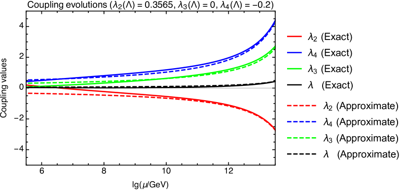
Refer to caption
Figure 6: Evolution of λ2subscript𝜆2\lambda_{2}, λ3subscript𝜆3\lambda_{3}, λ4subscript𝜆4\lambda_{4}, and λ𝜆\lambda in the 7-3-5 model for M35=105.5subscript𝑀35superscript105.5M_{35}=10^{5.5} GeV. The solid lines are the exact numerical solutions, while the dashed lines represent the approximate analytical solutions based on the assumption (63).

3.3.2 F0>0subscript𝐹00F_{0}>0

When F0>0subscript𝐹00{F_{0}}>0, the Landau pole of y𝑦y no longer exists. Instead, y𝑦y becomes a non-monotonic function of the energy scale μ𝜇\mu. It increases in the interval

M35μ<M35exp{8π2b2g22(0)[1(24F025b2)b2/(24+b2)]}subscript𝑀35𝜇subscript𝑀358superscript𝜋2subscript𝑏2superscriptsubscript𝑔220delimited-[]1superscript24subscript𝐹025subscript𝑏2subscript𝑏224subscript𝑏2\displaystyle M_{35}\leq\mu<M_{35}\exp\left\{\frac{8\pi^{2}}{b_{2}g_{2}^{2}(0)}\left[1-\left(\frac{24F_{0}}{25b_{2}}\right)^{b_{2}/(24+b_{2})}\right]\right\} (70)

and decreases in the interval

M35exp{8π2b2g22(0)[1(24F025b2)b224+b2]}μ<ΛLP(g2).subscript𝑀358superscript𝜋2subscript𝑏2superscriptsubscript𝑔220delimited-[]1superscript24subscript𝐹025subscript𝑏2subscript𝑏224subscript𝑏2𝜇superscriptsubscriptΛLPsubscript𝑔2\displaystyle M_{35}\exp\left\{\frac{8\pi^{2}}{b_{2}g_{2}^{2}(0)}\left[1-\left(\frac{24F_{0}}{25b_{2}}\right)^{\frac{b_{2}}{24+b_{2}}}\right]\right\}\leq\mu<\Lambda_{\mathrm{LP}}^{(g_{2})}. (71)

In the latter interval, y2superscript𝑦2y^{2} behaves as

24+b2F0(g2(t)g2(t0))48/b2g22(t0)24subscript𝑏2subscript𝐹0superscriptsubscript𝑔2superscript𝑡subscript𝑔2subscriptsuperscript𝑡048subscript𝑏2superscriptsubscript𝑔22subscriptsuperscript𝑡0\frac{24+b_{2}}{{F_{0}}}\left(\frac{g_{2}(t^{\prime})}{g_{2}(t^{\prime}_{0})}\right)^{-48/b_{2}}g_{2}^{2}(t^{\prime}_{0})

when g22g22(t0)much-greater-thansuperscriptsubscript𝑔22superscriptsubscript𝑔22subscriptsuperscript𝑡0g_{2}^{2}\gg g_{2}^{2}(t^{\prime}_{0}). It decrease very quickly and finally goes to zero. Then the 7-3-5 model essentially turns back to the SM+septuplet model at high energy scales. As we known, λ2subscript𝜆2\lambda_{2} and λ4subscript𝜆4\lambda_{4} will grow faster than g22superscriptsubscript𝑔22g_{2}^{2} and reach their Landau poles before ΛLP(g2)superscriptsubscriptΛLPsubscript𝑔2\Lambda_{\mathrm{LP}}^{(g_{2})}. To illustrate this more concretely, we will solve the RGEs at high energy scales. The equations are

d(g22)dt𝑑superscriptsubscript𝑔22𝑑superscript𝑡\displaystyle\frac{d(g_{2}^{2})}{dt^{\prime}} =\displaystyle= 2b2g24withb2=192,2subscript𝑏2superscriptsubscript𝑔24withsubscript𝑏2192\displaystyle 2b_{2}g_{2}^{4}~{}~{}\text{with}~{}~{}b_{2}=\frac{19}{2}, (72)
dλ2dt𝑑subscript𝜆2𝑑superscript𝑡\displaystyle\frac{d\lambda_{2}}{dt^{\prime}} =\displaystyle= 30λ22+452λ42+51λ2λ4144g22λ2,30superscriptsubscript𝜆22452superscriptsubscript𝜆4251subscript𝜆2subscript𝜆4144superscriptsubscript𝑔22subscript𝜆2\displaystyle 30\lambda_{2}^{2}+\frac{45}{2}\lambda_{4}^{2}+51\lambda_{2}\lambda_{4}-144g_{2}^{2}\lambda_{2}, (73)
dλ4dt𝑑subscript𝜆4𝑑superscript𝑡\displaystyle\frac{d\lambda_{4}}{dt^{\prime}} =\displaystyle= 288g24+2558λ42+24λ2λ4144g22λ4.288superscriptsubscript𝑔242558superscriptsubscript𝜆4224subscript𝜆2subscript𝜆4144superscriptsubscript𝑔22subscript𝜆4\displaystyle 288g_{2}^{4}+\frac{255}{8}\lambda_{4}^{2}+24\lambda_{2}\lambda_{4}-144g_{2}^{2}\lambda_{4}. (74)

We have neglected the 2λ322superscriptsubscript𝜆322\lambda_{3}^{2} term in Eq (73) but it would not affect the result a lot.

The things we would like to do is similar to the treatment in Ref. [17], but we include the running effect of g2subscript𝑔2g_{2} rather than treat g2subscript𝑔2g_{2} as constant. We assume that

λ2(t)=f1(t)g22(t),λ4(t)=f2(t)g22(t),formulae-sequencesubscript𝜆2superscript𝑡subscript𝑓1superscript𝑡superscriptsubscript𝑔22superscript𝑡subscript𝜆4superscript𝑡subscript𝑓2superscript𝑡superscriptsubscript𝑔22superscript𝑡\displaystyle\lambda_{2}(t^{\prime})=f_{1}(t^{\prime})g_{2}^{2}(t^{\prime}),~{}\lambda_{4}(t^{\prime})=f_{2}(t^{\prime})g_{2}^{2}(t^{\prime}), (75)

where f1,2(t)subscript𝑓12superscript𝑡f_{1,2}(t^{\prime}) are some functions of tsuperscript𝑡t^{\prime}. Substitute them into Eqs. (73)–(74), and we find

df1dG=30f12+452f22+51f1f2(144+2b2)f1,𝑑subscript𝑓1𝑑𝐺30superscriptsubscript𝑓12452superscriptsubscript𝑓2251subscript𝑓1subscript𝑓21442subscript𝑏2subscript𝑓1\displaystyle\frac{df_{1}}{dG}=30f_{1}^{2}+\frac{45}{2}f_{2}^{2}+51f_{1}f_{2}-(144+2b_{2})f_{1}, (76)
df2dG=288+2558f22+24f1f2(144+2b2)f2.𝑑subscript𝑓2𝑑𝐺2882558superscriptsubscript𝑓2224subscript𝑓1subscript𝑓21442subscript𝑏2subscript𝑓2\displaystyle\frac{df_{2}}{dG}=288+\frac{255}{8}f_{2}^{2}+24f_{1}f_{2}-(144+2b_{2})f_{2}. (77)

where dG=g22(t)dt𝑑𝐺superscriptsubscript𝑔22superscript𝑡𝑑superscript𝑡dG=g_{2}^{2}(t^{\prime})dt^{\prime}. The function G𝐺G can be easily obtained by integration and the result is

G(t)=1b2ln(g2(t)g2(t0)).𝐺superscript𝑡1subscript𝑏2subscript𝑔2superscript𝑡subscript𝑔2subscriptsuperscript𝑡0\displaystyle G(t^{\prime})=\frac{1}{b_{2}}\ln\left(\frac{g_{2}(t^{\prime})}{g_{2}(t^{\prime}_{0})}\right). (78)

The right hand side of Eq. (76) does not contain a constant, but the right hand side of Eq. (77) does.

We treat these equations in a way similar to what was did in Ref. [17]. Firstly, redefine f2subscript𝑓2f_{2} to remove the 24f1f224subscript𝑓1subscript𝑓224f_{1}f_{2} term. This can be done by linearly combining f1subscript𝑓1f_{1} and f2subscript𝑓2f_{2} as F=f1+ηf2𝐹subscript𝑓1𝜂subscript𝑓2F=f_{1}+\eta f_{2} with η=(17+7968)/641.66046𝜂177968641.66046\eta=(17+\sqrt{7968})/64\approx 1.66046. Then the equation of F𝐹F is

dFdG=c0c1F+c2F2+cf12,𝑑𝐹𝑑𝐺subscript𝑐0subscript𝑐1𝐹subscript𝑐2superscript𝐹2superscript𝑐superscriptsubscript𝑓12\frac{dF}{dG}=c_{0}-c_{1}F+c_{2}F^{2}+c^{\prime}f_{1}^{2}, (79)

where

c0subscript𝑐0\displaystyle c_{0} =\displaystyle= 288η478.212,c1=144+2b2=163,formulae-sequence288𝜂478.212subscript𝑐11442subscript𝑏2163\displaystyle 288\eta\approx 478.212,~{}c_{1}=144+2b_{2}=163, (80)
c2subscript𝑐2\displaystyle c_{2} =\displaystyle= 12(153+7969)7969+1727.3572,c=30c22.64278.formulae-sequence12153796979691727.3572superscript𝑐30subscript𝑐22.64278\displaystyle\frac{12(153+\sqrt{7969})}{\sqrt{7969}+17}\approx 27.3572,~{}c^{\prime}=30-c_{2}\approx 2.64278. (81)

The effect of cf12superscript𝑐superscriptsubscript𝑓12c^{\prime}f_{1}^{2} in Eq. (79) can be neglected because csuperscript𝑐c^{\prime} is small, and we can analytically solve the equation. The solution is

F(t)=c12c2+d^tan{c2d^G(t)+tan1[1d^(F(t0)c12c2)]},𝐹superscript𝑡subscript𝑐12subscript𝑐2^𝑑subscript𝑐2^𝑑𝐺superscript𝑡superscript11^𝑑𝐹subscriptsuperscript𝑡0subscript𝑐12subscript𝑐2F(t^{\prime})=\frac{c_{1}}{2c_{2}}+\hat{d}\tan\left\{c_{2}\hat{d}G(t^{\prime})+\tan^{-1}\left[\frac{1}{\hat{d}}\left(F(t^{\prime}_{0})-\frac{c_{1}}{2c_{2}}\right)\right]\right\}, (82)

with

d^=c0c2c124c222.93346.^𝑑subscript𝑐0subscript𝑐2superscriptsubscript𝑐124superscriptsubscript𝑐222.93346\hat{d}=\sqrt{\frac{c_{0}}{c_{2}}-\frac{c_{1}^{2}}{4c_{2}^{2}}}\approx 2.93346. (83)

Here t0subscriptsuperscript𝑡0t^{\prime}_{0} is chosen to correspond to a scale Λ0subscriptΛ0\Lambda_{0} where y(t0)𝑦subscriptsuperscript𝑡0y(t^{\prime}_{0}) is small compared to g2(t0)subscript𝑔2subscriptsuperscript𝑡0g_{2}(t^{\prime}_{0}). We can see that F(t)𝐹superscript𝑡F(t^{\prime}) diverges when

c2d^G(t)+tan1[1d^(F(t0)c12c2)]=π2.subscript𝑐2^𝑑𝐺superscript𝑡superscript11^𝑑𝐹subscriptsuperscript𝑡0subscript𝑐12subscript𝑐2𝜋2c_{2}\hat{d}G(t^{\prime})+\tan^{-1}\left[\frac{1}{\hat{d}}\left(F(t^{\prime}_{0})-\frac{c_{1}}{2c_{2}}\right)\right]=\frac{\pi}{2}.

It means for any initial value of F(t0)𝐹subscriptsuperscript𝑡0F(t^{\prime}_{0}), there always exists a Landau pole of F(t)𝐹superscript𝑡F(t^{\prime}) with a finite value of G(t)𝐺superscript𝑡G(t^{\prime}). This LP scale is

ΛLP(F)superscriptsubscriptΛLP𝐹\displaystyle\Lambda_{\mathrm{LP}}^{(F)} =\displaystyle= Λ0exp{8π2b2g22(t0)[1exp(b2πc2d^[12πtan1(F(t0)d^c12c2d^)])]}subscriptΛ08superscript𝜋2subscript𝑏2superscriptsubscript𝑔22subscript𝑡0delimited-[]1subscript𝑏2𝜋subscript𝑐2^𝑑delimited-[]12𝜋superscript1𝐹subscriptsuperscript𝑡0^𝑑subscript𝑐12subscript𝑐2^𝑑\displaystyle\Lambda_{0}\exp\left\{\frac{8\pi^{2}}{b_{2}g_{2}^{2}(t_{0})}\left[1-\exp\left(-\frac{b_{2}\pi}{c_{2}\hat{d}}\left[1-\frac{2}{\pi}\tan^{-1}\left(\frac{F(t^{\prime}_{0})}{\hat{d}}-\frac{c_{1}}{2c_{2}\hat{d}}\right)\right]\right)\right]\right\} (84)
=\displaystyle= ΛLP(g2)exp[8π2b2g22(t0)exp(b2πc2d^[12πtan1(F(t0)d^c12c2d^)])].superscriptsubscriptΛLPsubscript𝑔28superscript𝜋2subscript𝑏2superscriptsubscript𝑔22subscriptsuperscript𝑡0subscript𝑏2𝜋subscript𝑐2^𝑑delimited-[]12𝜋superscript1𝐹subscriptsuperscript𝑡0^𝑑subscript𝑐12subscript𝑐2^𝑑\displaystyle\Lambda_{\mathrm{LP}}^{(g_{2})}\exp\left[-\frac{8\pi^{2}}{b_{2}g_{2}^{2}(t^{\prime}_{0})}\exp\left(-\frac{b_{2}\pi}{c_{2}\hat{d}}\left[1-\frac{2}{\pi}\tan^{-1}\left(\frac{F(t^{\prime}_{0})}{\hat{d}}-\frac{c_{1}}{2c_{2}\hat{d}}\right)\right]\right)\right].

If we choose the range of y(0)𝑦0y(0) satisfying 25yc2/26y2(0)<yc225superscriptsubscript𝑦𝑐226superscript𝑦20superscriptsubscript𝑦𝑐225y_{c}^{2}/26\leq y^{2}(0)<y_{c}^{2} to make 0<F010subscript𝐹010<{F_{0}}\leq 1, we can assume that y𝑦y is small enough to be ignored in the running when the ratio

ξy2(t0)(24+b2)g22(t0)/25=[1+F025(g22(t0)g22(tf))(24+b2)/b2]1𝜉superscript𝑦2subscriptsuperscript𝑡024subscript𝑏2superscriptsubscript𝑔22subscriptsuperscript𝑡025superscriptdelimited-[]1subscript𝐹025superscriptsuperscriptsubscript𝑔22subscriptsuperscript𝑡0superscriptsubscript𝑔22subscriptsuperscript𝑡𝑓24subscript𝑏2subscript𝑏21\xi\equiv\frac{y^{2}(t^{\prime}_{0})}{(24+b_{2})g_{2}^{2}(t^{\prime}_{0})/25}=\left[1+\frac{{F_{0}}}{25}\left(\frac{g_{2}^{2}(t^{\prime}_{0})}{g_{2}^{2}(t^{\prime}_{f})}\right)^{(24+b_{2})/b_{2}}\right]^{-1}

is small enough. This will fix the value of g2(t0)subscript𝑔2subscriptsuperscript𝑡0g_{2}(t^{\prime}_{0}) by

1g22(t0)=1g22(0)[ξF025(1ξ)]b2/(24+b2).1superscriptsubscript𝑔22subscriptsuperscript𝑡01superscriptsubscript𝑔220superscriptdelimited-[]𝜉subscript𝐹0251𝜉subscript𝑏224subscript𝑏2\frac{1}{g_{2}^{2}(t^{\prime}_{0})}=\frac{1}{g_{2}^{2}(0)}\left[\frac{{\xi F_{0}}}{25(1-\xi)}\right]^{b_{2}/(24+b_{2})}. (85)

Notice that from the scale M35subscript𝑀35M_{35} to the scale Λ0subscriptΛ0\Lambda_{0}, the function of y(t)𝑦𝑡y(t) can be approximated by that in the F0=0subscript𝐹00{F_{0}}=0 limit. This means that in this scale range, the approximate solutions of λisubscript𝜆𝑖\lambda_{i} and λ𝜆\lambda to Eqs. (63) work well if Λ0subscriptΛ0\Lambda_{0} is high enough. Then we can estimate F(t0)𝐹subscriptsuperscript𝑡0F(t^{\prime}_{0}) by a1+ηa21.359subscript𝑎1𝜂subscript𝑎21.359a_{1}+\eta a_{2}\approx 1.359, and the LP scale is

ΛLP(F)superscriptsubscriptΛLP𝐹\displaystyle\Lambda_{\mathrm{LP}}^{(F)} \displaystyle\approx ΛLP(g2)exp[8π2b2g22(0)(ξF025(1ξ))b2/(24+b2)\displaystyle\Lambda_{\mathrm{LP}}^{(g_{2})}\exp\Bigg{[}-\frac{8\pi^{2}}{b_{2}g_{2}^{2}(0)}\left(\frac{{\xi F_{0}}}{25(1-\xi)}\right)^{b_{2}/(24+b_{2})} (86)
×exp(b2πc2d^[12πtan1(a1+ηa2c1/(2c2)d^)])].\displaystyle\qquad\qquad\qquad\times\exp\left(-\frac{b_{2}\pi}{c_{2}\hat{d}}\left[1-\frac{2}{\pi}\tan^{-1}\left(\frac{a_{1}+\eta a_{2}-c_{1}/(2c_{2})}{\hat{d}}\right)\right]\right)\Bigg{]}.\qquad

For F01subscript𝐹01F_{0}\leq 1, ξ=0.895𝜉0.895\xi=0.895 leads to an agreement with the full numerical calculation. We show the ratio ΛLP(g2)/ΛLP(F)superscriptsubscriptΛLPsubscript𝑔2superscriptsubscriptΛLP𝐹\Lambda_{\mathrm{LP}}^{(g_{2})}/\Lambda_{\mathrm{LP}}^{(F)} as a function of F0subscript𝐹0F_{0} in Fig. 7. We can see that for F0=1subscript𝐹01F_{0}=1, the LP scale of F𝐹F is smaller than ΛLP(g2)superscriptsubscriptΛLPsubscript𝑔2\Lambda_{\mathrm{LP}}^{(g_{2})} by 4 orders of magnitude. If one wants ΛLP(F)superscriptsubscriptΛLP𝐹\Lambda_{\mathrm{LP}}^{(F)} to be 101ΛLP(g2)similar-toabsentsuperscript101superscriptsubscriptΛLPsubscript𝑔2\sim 10^{-1}\Lambda_{\mathrm{LP}}^{(g_{2})}, F0subscript𝐹0F_{0} should be tuned to 0.002similar-toabsent0.002\sim 0.002, which is unnatural. For a larger F0subscript𝐹0{F_{0}}, ΛLP(F)superscriptsubscriptΛLP𝐹\Lambda_{\mathrm{LP}}^{(F)} is lower, because the 7-3-5 Yukawa coupling has smaller effect on the running of quartic couplings.

Refer to caption
Figure 7: The ratio ΛLP(g2)/ΛLP(F)superscriptsubscriptΛLPsubscript𝑔2superscriptsubscriptΛLP𝐹\Lambda_{\mathrm{LP}}^{(g_{2})}/\Lambda_{\mathrm{LP}}^{(F)} as a function of F0subscript𝐹0{F_{0}} in the range 0<F010subscript𝐹010<{F_{0}}\leq 1.

4 Conclusions and discussions

Perturbativity yields strong bounds on the MDM model, but most of the previous studies only consider the gauge couplings and conclude that the real scalar septuplet MDM model can keep perturbative up to the Planck scale. In this article we take into account the quartic self-interactions of the real scalar septuplet in the septuplet MDM model, and find that for an MDM particle mass of 10similar-toabsent10\sim 10 TeV the Landau poles of the quartic couplings appear around 108superscript10810^{8} GeV, which is consistent with the approximate analytical treatment in Ref. [17].

As an attempt to push up the LP scale, we propose an extension to the model with Yukawa interactions among the septuplet, an extra fermionic quintuplet, and one or two extra fermionic triplets. In principle, the Landau pole can be deferred to appear at 1014superscript101410^{14} GeV, but it is at the price of a serious fine-tuning of the initial condition of the new Yukawa coupling. We investigate the evolution of couplings up to a scale just a little bit below the highest possible LP scale, and use the VS and perturbativity conditions to constrain the quartic couplings. It is found that the Higgs portal coupling has an acceptable range of 0.25<λ3<10.25subscript𝜆31-0.25<\lambda_{3}<1. Moreover, if the MDM particle mass could be relaxed to 108similar-toabsentsuperscript108\sim 10^{8} GeV, which demands some nonthermal production mechanisms, we could push up the LP scale even beyond the Planck scale.

In a scalar MDM model with doublet, triplet, or quadruplet, the couplings can remain perturbative up to the Planck scale. On the other hand, when the MDM scalar multiplet lives in an SU(2)L𝑆𝑈subscript2𝐿SU(2)_{L} representation with a dimension higher than 5, the scalar MDM model would have Landau poles appearing before the Planck scale, due to the MDM framework, i.e., the MDM particle mass fixed by thermal freeze-out dynamics. As what we propose in this article, these models may be cured as well by introducing extra Yukawa couplings. We leave this possibility to a specific study [37].

Acknowledgments

This work is supported by the National Natural Science Foundation of China (NSFC) under Grant Nos. 11375277, 11410301005, and 11005163, the Fundamental Research Funds for the Central Universities, and the Sun Yat-Sen University Science Foundation.

References

  • [1] M. Cirelli, N. Fornengo and A. Strumia, Minimal dark matter, Nucl. Phys. B 753, 178 (2006) [hep-ph/0512090].
  • [2] M. Cirelli, A. Strumia and M. Tamburini, Cosmology and Astrophysics of Minimal Dark Matter, Nucl. Phys. B 787, 152 (2007) [arXiv:0706.4071 [hep-ph]].
  • [3] M. Cirelli and A. Strumia, Minimal Dark Matter: Model and results, New J. Phys.  11, 105005 (2009) [arXiv:0903.3381 [hep-ph]].
  • [4] T. Hambye, F.-S. Ling, L. Lopez Honorez and J. Rocher, Scalar Multiplet Dark Matter, JHEP 0907, 090 (2009) [Erratum-ibid.  1005, 066 (2010)] [arXiv:0903.4010 [hep-ph]].
  • [5] F. S. Ling, Heavy Scalar Dark Matter, arXiv:0905.4823 [hep-ph].
  • [6] K. Earl, K. Hartling, H. E. Logan and T. Pilkington, Constraining models with a large scalar multiplet, Phys. Rev. D 88, 015002 (2013) [arXiv:1303.1244 [hep-ph]].
  • [7] M. Cirelli, R. Franceschini and A. Strumia, Minimal Dark Matter predictions for galactic positrons, anti-protons, photons, Nucl. Phys. B 800, 204 (2008) [arXiv:0802.3378 [hep-ph]].
  • [8] M. Cirelli and A. Strumia, Minimal Dark Matter predictions and the PAMELA positron excess, PoS IDM 2008, 089 (2008) [arXiv:0808.3867 [astro-ph]].
  • [9] M. Cirelli, T. Hambye, P. Panci, F. Sala and M. Taoso, Gamma ray tests of Minimal Dark Matter, arXiv:1507.05519 [hep-ph].
  • [10] C. Garcia-Cely, A. Ibarra, A. S. Lamperstorfer and M. H. G. Tytgat, Gamma-rays from Heavy Minimal Dark Matter, arXiv:1507.05536 [hep-ph].
  • [11] M. R. Buckley, L. Randall and B. Shuve, LHC Searches for Non-Chiral Weakly Charged Multiplets, JHEP 1105, 097 (2011) [arXiv:0909.4549 [hep-ph]].
  • [12] Y. Cai, W. Chao and S. Yang, Scalar Septuplet Dark Matter and Enhanced hγγ𝛾𝛾h\rightarrow\gamma\gamma Decay Rate, JHEP 1212, 043 (2012) [arXiv:1208.3949 [hep-ph]].
  • [13] M. Cirelli, F. Sala and M. Taoso, Wino-like Minimal Dark Matter and future colliders, JHEP 1410, 033 (2014) [JHEP 1501, 041 (2015)] [arXiv:1407.7058 [hep-ph]].
  • [14] K. Harigaya, K. Ichikawa, A. Kundu, S. Matsumoto and S. Shirai, Indirect Probe of Electroweak-Interacting Particles at Future Lepton Colliders, JHEP 1509, 105 (2015) [arXiv:1504.03402 [hep-ph]].
  • [15] B. Ostdiek, Constraining the minimal dark matter fiveplet with LHC searches, arXiv:1506.03445 [hep-ph].
  • [16] L. Di Luzio, R. Gröber, J. F. Kamenik and M. Nardecchia, Accidental matter at the LHC, JHEP 1507, 074 (2015) [arXiv:1504.00359 [hep-ph]].
  • [17] Y. Hamada, K. Kawana and K. Tsumura, Landau pole in the Standard Model with weakly interacting scalar fields, Phys. Lett. B 747, 238 (2015) [arXiv:1505.01721 [hep-ph]].
  • [18] R. Foot, H. Lew, X. G. He and G. C. Joshi, Seesaw Neutrino Masses Induced by a Triplet of Leptons, Z. Phys. C 44, 441 (1989).
  • [19] P. A. R. Ade et al. [Planck Collaboration], Planck 2015 results. XIII. Cosmological parameters, arXiv:1502.01589 [astro-ph.CO].
  • [20] J. R. Ellis, A. Ferstl and K. A. Olive, Reevaluation of the elastic scattering of supersymmetric dark matter, Phys. Lett. B 481, 304 (2000) [hep-ph/0001005].
  • [21] D. S. Akerib et al. [LUX Collaboration], First results from the LUX dark matter experiment at the Sanford Underground Research Facility, Phys. Rev. Lett.  112, 091303 (2014) [arXiv:1310.8214 [astro-ph.CO]].
  • [22] M. Cirelli et al., PPPC 4 DM ID: A Poor Particle Physicist Cookbook for Dark Matter Indirect Detection, JCAP 1103, 051 (2011) [JCAP 1210, E01 (2012)] [arXiv:1012.4515 [hep-ph]].
  • [23] M. Ackermann et al. [Fermi-LAT Collaboration], Searching for Dark Matter Annihilation from Milky Way Dwarf Spheroidal Galaxies with Six Years of Fermi-LAT Data, arXiv:1503.02641 [astro-ph.HE].
  • [24] K. Kannike, Vacuum Stability Conditions From Copositivity Criteria, Eur. Phys. J. C 72, 2093 (2012) [arXiv:1205.3781 [hep-ph]].
  • [25] T. P. Cheng, E. Eichten and L. F. Li, Higgs Phenomena in Asymptotically Free Gauge Theories, Phys. Rev. D 9, 2259 (1974).
  • [26] F. Lyonnet, I. Schienbein, F. Staub and A. Wingerter, PyR@TE: Renormalization Group Equations for General Gauge Theories, Comput. Phys. Commun.  185, 1130 (2014) [arXiv:1309.7030 [hep-ph]].
  • [27] J. Beringer et al. [Particle Data Group Collaboration], Review of Particle Physics, Phys. Rev. D 86 (2012) 010001.
  • [28] T. Hambye and K. Riesselmann, Matching conditions and Higgs mass upper bounds revisited, Phys. Rev. D 55, 7255 (1997) [hep-ph/9610272].
  • [29] Y. Cai, X. G. He, M. Ramsey-Musolf and L. H. Tsai, Rν𝜈\nuMDM and Lepton Flavor Violation, JHEP 1112, 054 (2011) [arXiv:1108.0969 [hep-ph]].
  • [30] K. Kumericki, I. Picek and B. Radovcic, Critique of Fermionic Rν𝜈\nuMDM and its Scalar Variants, JHEP 1207, 039 (2012) [arXiv:1204.6597 [hep-ph]].
  • [31] P. Culjak, K. Kumericki and I. Picek, Scotogenic Rν𝜈\nuMDM at three-loop level, Phys. Lett. B 744, 237 (2015) [arXiv:1502.07887 [hep-ph]].
  • [32] E. Witten, An SU(2) Anomaly, Phys. Lett. B 117 (1982) 324.
  • [33] O. Bar, On Witten’s global anomaly for higher SU(2) representations, Nucl. Phys. B 650 (2003) 522 [hep-lat/0209098].
  • [34] M. Aoki, T. Toma and A. Vicente, Non-thermal Production of Minimal Dark Matter via Right-handed Neutrino Decay, arXiv:1507.01591 [hep-ph].
  • [35] D. J. H. Chung, E. W. Kolb and A. Riotto, Superheavy dark matter, Phys. Rev. D 59, 023501 (1999) [hep-ph/9802238].
  • [36] A. Falkowski and J. M. No, Non-thermal Dark Matter Production from the Electroweak Phase Transition: Multi-TeV WIMPs and ’Baby-Zillas’,’ JHEP 1302, 034 (2013) [arXiv:1211.5615 [hep-ph]].
  • [37] C. Cai, Z. M. Huang, Z. Kang, Z. H. Yu and H. H. Zhang, in preparation.