Optimal Fronthaul Compression for Synchronization in the Uplink of Cloud Radio Access Networks

Abstract

A key problem in the design of cloud radio access networks (CRANs) is that of devising effective baseband compression strategies for transmission on the fronthaul links connecting a remote radio head (RRH) to the managing central unit (CU). Most theoretical works on the subject implicitly assume that the RRHs, and hence the CU, are able to perfectly recover time synchronization from the baseband signals received in the uplink, and focus on the compression of the data fields. This paper instead dose not assume a priori synchronization of RRHs and CU, and considers the problem of fronthaul compression design at the RRHs with the aim of enhancing the performance of time and phase synchronization at the CU. The problem is tackled by analyzing the impact of the synchronization error on the performance of the link and by adopting information and estimation-theoretic performance metrics such as the rate-distortion function and the Cramer-Rao bound (CRB). The proposed algorithm is based on the Charnes-Cooper transformation and on the Difference of Convex (DC) approach, and is shown via numerical results to outperform conventional solutions.

I Introduction

As mobile operators are faced with increasingly demanding requirements in terms of data rates and operational costs, the novel architecture of cloud radio access networks (C-RANs) has emerged as a promising solution [1],[2]. In a C-RAN, the baseband processing of the base stations is migrated to a central unit (CU) in the “cloud", to which the base station, typically referred to an remote radio heads (RRHs), are connected via fronthaul links, which in turn may be realized via fiber optics, microwave or mmwave technologies. By simplifying the network edge and by centralizing baseband processing, the C-RAN architecture is expected to provide significant benefits in energy efficiency, load balancing, and interference management capabilities (see review in [2])

A key problem in C-RANs is that of devising effective baseband compression methods in order to cope with the limitation in the capacity of the fronthaul links. Most theoretical works on the subject implicitly assume perfect time synchronization and channel state

information (CSI) at the RRHs and the CU (see, e.g., [2][8]). However, on the one hand, this assumption violates the C-RAN paradigm that minimal baseband processing should be carried out at the BSs, and, on the other hand, the resulting design neglects the additional requirements on fronthaul processing at the RRHs that are imposed by synchronization and channel estimation. This limitation is alleviated by [5], which considers robust compression in the presence of imperfect CSI, and by papers [6][7], which study the impact of fronthaul compression on channel estimation. To the best of our knowledge, analysis that account for imperfect time synchronization are instead not available.

In this paper, we consider training-based synchronization for the uplink of a C-RAN cellular system. Specifically, we investigate the problem of optimal fronthaul compression of the training field with the aim of enhancing the performance of time and phase synchronization at the CU. To this end, the effect of the synchronization error on the signal to noise ratio (SNR) is analyzed by adopting the Cramer-Rao bound (CRB) as the performance criterion of interest and by accounting for compression via information theoretic tools. The resulting proposed algorithm is based on the Charnes-Cooper transformation [9] and the Difference of Convex (DC) approach [10]. Numerical results show that optimized fronthaul compression that targets enhanced synchronization performance outperforms conventional solution that do not account for the impact of synchronization errors. The rest of the paper is organized as follows. Sec. II introduce system model of uplink C-RAN cellular system. The analytic study of the performance and optimization are presented in Sec. III: the CRBs of time and phase offset estimation carried at CU is derived in Sec. III-A, and the analysis of impact of the synchronization error on the effective SNR in Sec. III-B, and the optimization of fronthaul compression in Sec. III-C. Finally, the performance is evaluated through simulations to present benefits of the proposed compression scheme in Sec. IV.

II System model

In this paper, we consider training-based synchronization for the uplink of a C-RAN cellular system. We specifically focus on the operation of a single cell, as illustrated in Fig. 1, and assume that, as in current cellular implementations, the MSs transmit over orthogonal time/frequency resources, so that we can focus on a single active MS in a given resource block. The MS transmits a frame consisting of a training and a data field. We further assume that the active MS and the RRH have a single antenna. The RRH is connected to a CU via a fronthaul link that can deliver $C$ bits per uplink sample to the CU. It is also assumed that the RRH is synchronized at the frame level so as to be able to distinguish between the training and data fields that compose each transmitted frame.

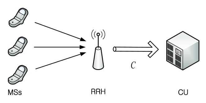
Figure 1: Uplink communication between a number of MSs and an RRH. The RRH is connected via a finite-capacity fronthaul link to a CU that performs baseband processing, including synchronization.

II-A Training Phase

Assuming a flat-fading channel, the signal received at the RRH during the training, or pilot, field, is given as

$$y_{p}(t) =Ae^{j\theta}\sum_{l=-L+1}^{N_{p}-1}x_{p}[l]g(t-lT-\tau)+z_{p}(t),\ t\in[0,N_{p}T),$$ (1)

where $A$ is a positive amplitude that accounts for the attenuation due to fading; $\theta$ is the phase offset, which models the effect of the channel and of the phase mismatch between the oscillators at the MS and at the RRH; $\tau$ accounts for the residual timing offset between MS and RRH; $T$ is the symbol period; $x_{p}[l]$ is the $l$th pilot symbol transmitted by the MS; $N_{p}$ is the number of pilot symbols; $g(t)$ is the pulse shape, which includes the effect of the transmit and receive filter and is assumed to be supported in the interval $[0,(L-1)T]$ for some integer $L>1$; and $z_{p}(t)$ is the complex additive white Gaussian noise with two-sided power spectral density $N_{0}$. We assume that the RRH is able to estimate the channel amplitude $A$, for instance, by means of automatic gain control in the presence of constant amplitude symbols. Instead, the time offset $\tau$ and phase offset $\theta$ need to be estimated from the received signal (1).

The training sequence is generated randomly such that the symbols $x_{p}[l]$ for $l=0,...,N_{p}-1$ are independent and distributed as $\mathcal{CN}(0,E_{x_{p}})$. The training sequence is known to the CU and the random generation is assumed here for the sake of simplifying the analysis in the spirit of Shannon’s random coding (see, e.g., [11]). We further assume that the pilot symbols are preceded by a cyclic prefix of duration equal to $(L-1)T$. This implies that $x_{p}[-l]=x_{p}[-l+N_{p}]$ for $1\leq l\leq L-1$. Alternatively, as it will be discussed, the analysis below holds as long as the number of training symbols $N_{p}$ is sufficiently larger than the support of the waveform $g(t)$ $L$.

In order to potentially enhance the performance of phase and time synchronization, we allow the receiver to oversample the received signal at the BS with a sampling period $T_{s}=T/F$, where $F$ is the oversampling factor. We assume for simplicity of analysis that a raised cosine pulse $g(t)$ with zero excess bandwidth (i.e., a sinc function) is used, so that the two-sided bandwidth is $B=1/T$. As a result, setting $F=1$, i.e., no oversampling, is an acceptable choice that leads to no spectral aliasing. However, as it will be seen in Sec IV, the selection $F>1$ may yield an improved performance. The resulting discrete-time signal $y_{p}(mT+nT_{s})$ can be expressed as the interleaving of the $F$ polyphase sequences $y^{n}_{p}[m]=y_{p}(mT+nT_{s})$, with $n=0,1,...,F-1$, see, e.g., [12]. Each sequence $y^{n}_{p}[m]$ can be in turn written as

$$y^{n}_{p}[m] =Ax_{p}[m]\circledast g_{\tau,\theta}^{n}[m]+z^{n}_{p}[m],\ \ m=0,...,N_{p}-1,$$ (2)

where we have defined $z^{n}_{p}[m]\triangleq z_{p}(mT+nT_{s})$, $g_{\tau,\theta}^{n}[m]\triangleq e^{j\theta}g(mT+nT_{s}-\tau)$, and $\circledast$ denotes the circular convolution. Assuming that the noise $z_{p}(t)$ is white over the bandwidth $[-1/{2T_{s}},1/{2T_{s}}]$, the discrete-time noise sequence $z^{n}_{p}[m]$ is an i.i.d. process with zero mean and power $N_{0}/T_{s}$.

Remark 1.

Due to receive-side filtering, the noise is more properly modelled as being bandlimited with the same bandwidth of the signal. In this case, the discrete-time noise is actually correlated across time for $F>1$. Here, following many related references (see, e.g., [13][14]), we instead make the simplifying assumption that the noise is white. This choice can be seen to lead to lower bounds on the actual system performance. $\Box$

II-B Data Phase

The signal received during the data field of a frame can be written, in an analogous fashion as (1), as

$$y_{d}(t) =Ae^{j\theta}\sum_{l=-L+1}^{N_{d}-1}x_{d}[l]g(t-lT-\tau)+z_{d}(t),\ t\in[0,N_{d}T),$$ (3)

where $x_{d}[l]$ is the $l$th data symbol transmitted by the MS, which is generated randomly in a constellation set $\Omega_{x}$ with zero mean and power $E_{x_{d}}$, and $N_{d}$ is the number of data symbols. The other parameters are defined as in (1). Moreover, as in (1), we assume that the symbol indexed as $l=-L+1,...,0$ amount to a cyclic prefix, or that $N_{p}$ is sufficiently larger than $L$. After sampling at baud rate for the data field, the discrete-time signal is given as

$$y_{d}[m] =Ae^{j\theta}\sum_{l=-L+1}^{N_{d}-1}x_{d}[l]g((m-l)T-\tau)+z_{d}[m],\ \ m=0,...,N_{d}-1,$$ (4)

where the discrete-time noise sequence $z_{d}[m]$ is an i.i.d. process with zero mean and power $N_{0}/T$. Note that oversampling could be adopted also for the data field by following the some model used for the training filed, but we do not further pursue this here in order to focus on training for synchronization.

II-C Fronthaul Compression

Following the C-RAN principle, compression is performed at the RRH in order to convey the baseband signal over the limited-capacity fronthaul link to the CU. For the training field, we assume the use of block quantizers that compress each $n$th polyphase sequence $y^{n}[m]$, with $n=0,...,F-1$, separately for transmission over the fronthaul link. Note that, while joint compression of these sequences generally leads to an improved compression efficiency, here we adopt separate compression both for its lower computation complexity and for its analytical tractability. Using the standard additive quantization noise model, the resulting compressed signal for each $n$th polyphase sequence can be written as

$$\hat{y}^{n}_{p}[m] =y^{n}_{p}[m]+q^{n}_{p}[m],\ \ \ m=0,...,N_{p}-1,$$ (5)

where $q^{n}_{p}[m]$ indicates the quantization noise. Noise $q^{n}_{p}[m]$ is assumed, for simplicity of analysis, to be complex Gaussian and generally correlated across the discrete-time index $m$. From the covering lemma of rate-distortion theory [11], vector quantization schemes can be designed such that the joint (empirical) distribution of the input and output of the quantizer satisfies (5), as long as the rate is sufficiently large (see, e.g., [11]). Furthermore, the relationship (5) can be in practice approximated by a high-dimensional dithered vector quantizers [15]. The practical relevance of the additive-noise quantization model for system design is further validated in Sec. IV by means of numerical results.

The covariance matrix $\textbf{K}_{\textbf{q}^{n}}$ of the vector $\textbf{q}^{n}_{p}=[q^{n}_{p}[0],...,q^{n}_{p}[N_{p}-1]]$ is taken to be circulant in order to facilitate its optimization in the frequency domain as discussed in the next section. Due to the separate quantization of the polyphase sequences, the quantization noise is independent across the index $n$.

Taking the Discrete Fourier Transform (DFT) of (5) leads to the frequency-domain signals

$$\hat{Y}^{n}_{p}[k] =AX_{p}[k]G^{n}_{\tau,\theta}[k]+Z^{n}_{p}[k]+Q^{n}_{p}[k],\ \ k=0,...,N_{p}-1,$$ (6)

where $X_{p}[k]$, $G^{n}_{\tau,\theta}[k]$, $Z^{n}_{p}[k]$, and $Q^{n}_{p}[k]$ are obtained by taking the DFT of the sequences $\{x_{p}[m]\}_{m=0}^{N_{p}-1}$, $\{g^{n}_{\tau,\theta}[m]\}_{m=0}^{N_{p}-1}$, $\{z^{n}_{p}[m]\}_{m=0}^{N_{p}-1}$, and $\{q^{n}_{p}[m]\}_{m=0}^{N_{p}-1}$, respectively. Due to the lack of spectral aliasing afforded by the chosen waveform and sampling frequency, we can write $G^{n}_{\tau,\theta}[k]=G^{n}[k]e^{-j(2\pi\frac{k}{N_{p}T_{s}}\tau-\theta)}$.

From the mentioned covering lemma [11] (see also [15]), the fronthaul rate required to convey the compressed signals $\hat{\textbf{y}}_{p}=[\hat{\textbf{y}}_{p}^{0},...,\hat{\textbf{y}}_{p}^{F-1}]$, where $\hat{\textbf{y}}_{p}^{n}=[\hat{y}^{n}_{p}[0],...,\hat{y}^{n}_{p}[N_{p}-1]]$, from the RRH to the CU is given by the mutual information $I(\textbf{y}_{p};\hat{\textbf{y}}_{p})$, with vector $\textbf{y}_{p}$ being similarly defined. However, the mutual information $I(\textbf{y}_{p};\hat{\textbf{y}}_{p})$ depends on the joint distribution of $\textbf{y}_{p}$ and $\hat{\textbf{y}}_{p}$ and hence on the timing offset $\tau$ and phase offset $\theta$, which are not known at the RRH. Therefore, the necessary rate of a worst-case estimate is $R_{p}=\sup_{\tau,\theta}I(\textbf{y}_{p};\hat{\textbf{y}}_{p})$. It can be easily calculated that the mutual information is given by

$$I(\textbf{y}_{p};\hat{\textbf{y}}_{p})=\sum^{F-1}_{n=0}\log_{2}\frac{|\textbf{K}_{\textbf{y}^{n}_{p}}+\textbf{K}_{\textbf{q}^{n}_{p}}|}{|\textbf{K}_{\textbf{q}^{n}_{p}}|},$$ (7)

where $\textbf{y}^{n}_{p}=[y^{n}_{p}[0],...,y^{n}_{p}[N_{p}-1]]$. Since the covariance matrix of the quantization noise $\textbf{K}_{\textbf{q}^{n}_{p}}$ is assumed to be circulant, by leveraging Szeg$\ddot{\textrm{o}}$ theorem [16], we can write (7) as

$$I(\textbf{y}_{p};\hat{\textbf{y}}_{p})=\sum_{n=0}^{F-1}\sum_{k=0}^{N_{p}-1}\log_{2}\left(1+\frac{E_{x_{p}}A^{2}|G^{n}[k]|^{2}+N_{0}/T_{s}}{S_{Q^{n}_{p}}[k]}\right),$$ (8)

where $S_{Q^{n}_{p}}[k]$, for $k=0,...,N_{p}-1$, indicate the eigenvalues of the matrix $\textbf{K}_{\textbf{q}^{n}_{p}}$. We will refer to $S_{Q^{n}_{p}}[k]$ as the power spectral density (PSD) of the quantization noise $q^{n}_{p}[m]$. We observe that (8) does not depend on $\theta$ and $\tau$. Therefore, the required fronthaul rate $R_{p}$ is given by the right-hand side of (8). We will therefore impose the fronthaul capacity constraint as

$$I(\textbf{y}_{p};\hat{\textbf{y}}_{p})\leq N_{p}C,$$ (9)

where $I(\textbf{y}_{p};\hat{\textbf{y}}_{p})$ is given in (8).

The compressed data signal during the data field, similar to (5), can be written as

$$\hat{y}_{d}[m] =y_{d}[m]+q_{d}[m],\ \ m=0,...,N_{d}-1.$$ (10)

where $q_{d}[m]$ indicates the quantization noise, which is assumed to be white Gaussian random variable with zero mean and variance $\sigma^{2}_{q_{d}}$. We observe that an optimized correlation for the quantization noise on the data phase could also be designed, similar to [5], but we leave this aspect to future work in order to concentrate on training for synchronization. Furthermore, following the discussion above, the fronthaul rate required to convey the compressed data signal $\hat{\textbf{y}}_{d}=[\hat{y}_{d}[0],...,\hat{y}_{d}[N_{d}-1]]$, from the RRH to the CU is given by $R_{d}=\sup_{\tau,\theta}I(\textbf{y}_{d};\hat{\textbf{y}}_{d})$, with vector $\textbf{y}_{d}$ being similarly defined, with

$$I(\textbf{y}_{d};\hat{\textbf{y}}_{d}) =\log_{2}\frac{|\textbf{K}_{\textbf{y}_{d}}+\textbf{K}_{\textbf{q}_{d}}|}{|\textbf{K}_{\textbf{q}_{d}}|},$$ (11a)

$$=\sum_{i=0}^{N_{d}-1}\log_{2}\left(1+\frac{E_{x_{d}}A^{2}|G[i]|^{2}+N_{0}}{\sigma^{2}_{q_{d}}}\right),$$ (11b)

where (11b) follows from Szeg$\ddot{\textrm{o}}$ theorem as in (8) and the fronthaul capacity constraint of the data phase is given as

$$I(\textbf{y}_{d};\hat{\textbf{y}}_{d})\leq N_{d}C.$$ (12)

III Analysis and Optimization

In this section, we analyze the performance of the C-RAN system introduced above by accounting for the impact of imperfect synchronization, with the aim of enabling the optimization of fronthual quantization. We will first discuss the performance of time and phase synchronization at the CU in Section III-A. Then, we study the impact of synchronization errors on the SNR in Section III-B. Finally, we investigate the optimization of fronthual compression in Section III-C.

III-A CRBs for Time and Phase Offset Estimation

The CU estimates the time and phase offsets based on the compressed pilot signals $\hat{\textbf{y}}_{p}$, producing the estimates $\hat{\tau}(\hat{\textbf{y}}_{p},\textbf{x}_{p})$ and $\hat{\theta}(\hat{\textbf{y}}_{p},\textbf{x}_{p})$. The mean squared errors (MSEs) of these estimates can be bounded by the corresponding CRBs i.e., by the inequalities $E_{\hat{\textbf{{y}}}_{p},\textbf{x}_{p}}[(\hat{\tau}(\hat{\textbf{y}}_{p},\textbf{x}_{p})-\tau)^{2}]\geq\textrm{CRB}_{\tau}$ and $E_{\hat{\textbf{{y}}}_{p},\textbf{x}_{p}}[(\hat{\theta}(\hat{\textbf{y}}_{p},\textbf{x}_{p})-\theta)^{2}]\geq\textrm{CRB}_{\theta}$. Note that the mentioned estimates depend on both the training sequence $\textbf{x}_{p}$ and the compressed received signal $\hat{\textbf{y}}_{p}$, and that the squared error is averaged over the joint distribution of $\textbf{x}_{p}$ and $\hat{\textbf{y}}_{p}$. To evaluate the CRBs, we assume that the relationship (5)-(6) is satisfied for the given vector quantizer. This is done for the sake of tractability and is motivated by the covering lemma and by the results in [15] as discussed in the previous section. The CRBs are given, respectively, as

$$\textrm{CRB}_{\tau} =\left(\left(\frac{2\pi}{N_{p}T_{s}}\right)^{2}\sum_{n=0}^{F-1}\sum_{k=0}^{N_{p}-1}\frac{E_{x_{p}}A^{2}k^{2}|G^{n}[k]|^{2}}{\frac{N_{0}}{T_{s}}+S_{Q^{n}_{p}}[k]}\right)^{-1},$$ (13)

and

$$\textrm{CRB}_{\theta} =\left(\sum_{n=0}^{F-1}\sum_{k=0}^{N_{p}-1}\frac{E_{x_{p}}|A|^{2}|G^{n}[k]|^{2}}{\frac{N_{0}}{T_{s}}+S_{Q^{n}_{p}}[k]}\right)^{-1}.$$ (14)

Given (5)-(6), the derivation of (13)-(14) follows from standard arguments, see, e.g., [17]. Note that the bounds (13) and (14) do not depend on the phase $\theta$ and delay $\tau$.

III-B Impact of the Synchronization Error on the SNR

Having estimated the time and phase offsets $\hat{\tau}$ and $\hat{\theta}$, the CU compensates for these offsets the received signal (15), obtaining the discrete-time signal

$$y_{d}[m] =Ae^{j\Delta\theta}\sum_{l=-L+1}^{N_{d}-1}x_{d}[l]g((m-l)T+\Delta\tau)+z_{d}[m],\ \ m=0,...,N_{d}-1,$$ (15)

where $\Delta\tau=\hat{\tau}(\hat{\textbf{y}},\textbf{x})-\tau$ and $\Delta\theta=\hat{\theta}(\hat{\textbf{y}},\textbf{x})-\theta$ are the synchronization errors for timing and phase, respectively. We note that compensation of the time offset requires interpolation, which is possible given the lack of spectral aliasing. Moreover, under the mentioned assumption on the zero excess bandwidth waveform $g(t)$, the statistics of the (white Gaussian) noise terms are unchanged by interpolation.

To account for the impact of the synchronization errors $\Delta\tau$ and $\Delta\theta$, we follow the approach in [18], whereby the sinc waveform $g(t)$ is approximated by retaining only two sidelobes on either side. Under this approximation, we can express (15) as

$$y_{d}[m]=Ax_{d}[m]g(\Delta\tau)+z_{s}[m]+z_{isi}[m]+z_{d}[m],$$ (16)

where the terms in (16) are detailed below. First, the term $z_{s}[m]=Ax_{d}[m]g(\Delta\tau)(e^{j\Delta\theta}-1)$ indicates additional noise caused by the estimation error of phase offset $\Delta\theta$. The term $z_{isi}[m]$ instead accounts for inter-symbol interference caused by the time synchronization error and is given as

$$z_{isi}[m]=Ae^{j\Delta\theta}\sum_{l=m-3,l\neq m}^{l=m+3}x_{d}[l]g((l-m)T+\Delta\tau).$$ (17)

In order to evaluate the power of the noise terms $z_{s}[m]$ and $z_{isi}[m]$, we make the simplifying assumption that the estimation errors $\Delta\tau$ and $\Delta\theta$ are uniform distributed on $[-\frac{\Delta\tau_{\textrm{max}}}{2},\frac{\Delta\tau_{\textrm{max}}}{2}]$ and on $[-\frac{\Delta\theta_{\textrm{max}}}{2},\frac{\Delta\theta_{\textrm{max}}}{2}]$, respectively. We observe that this approximation is expected to be increasingly accurate in the regime of small synchronization errors. Moreover, we approximate $\Delta\tau_{\textrm{max}}$ and $\Delta\theta_{\textrm{max}}$ by means of the $\textrm{CRB}_{\tau}$ (13) and $\textrm{CRB}_{\theta}$ (14), respectively, by imposing the equalities $E[\Delta\tau^{2}]=\textrm{CRB}_{\tau}$ and $E[\Delta\theta^{2}]=\textrm{CRB}_{\theta}$, which yields $\Delta\tau_{\textrm{max}}=\sqrt{12\textrm{CRB}_{\tau}}$ and $\Delta\theta_{\textrm{max}}=\sqrt{12\textrm{CRB}_{\theta}}$. Finally, we adopt the piecewise linear approximation of the raised cosine pulse $g(t)$ proposed in [18], whereby pulse $g(t)$ can be written as

$$g((l-m)T+\Delta\tau)\approx\ a_{l}\times\frac{\Delta\tau}{T},$$ (18a)

where $$a_{l}=a_{l}^{+}\ \ \textrm{if}\ \Delta\tau>0$$ (18b)

and $$a_{l}=a_{l}^{-}\ \ \textrm{if}\ \Delta\tau<0,$$ (18c)

for $l\neq m$ and

$$g(\Delta\tau)\approx\left(1-\eta\frac{|\Delta\tau|}{T}\right),$$ (19)

where we have defined $\eta=\frac{2T}{\Delta\tau_{\textrm{max}}}(1-g(\Delta\tau_{\textrm{max}}/2T))$ and the values of $a_{l}^{+}$ and $a_{l}^{-}$ are listed in Table I, in which we have $c_{1}=\frac{2T}{\Delta\tau_{\textrm{max}}}g(1-\frac{\Delta\tau_{\textrm{max}}}{2T})$, $c_{2}=\frac{2T}{\Delta\tau_{\textrm{max}}}|g(1+\frac{\Delta\tau_{\textrm{max}}}{2T})|$, $c_{3}=\frac{2T}{\Delta\tau_{\textrm{max}}}|g(2-\frac{\Delta\tau_{\textrm{max}}}{2T})|$, $c_{4}=\frac{2T}{\Delta\tau_{\textrm{max}}}g(2+\frac{\Delta\tau_{\textrm{max}}}{2T})$, and $c_{5}=\frac{2T}{\Delta\tau_{\textrm{max}}}g(3-\frac{\Delta\tau_{\textrm{max}}}{2T})$ [18].

TABLE I: Coefficients in the piecewise linear approximation of the raised cosine pulse

$l$	$m-3$	$m-2$	$m-1$	$m+1$	$m+2$	$m+3$
$a^{+}_{l}$	$0$	$c_{4}$	$-c_{2}$	$c_{1}$	$-c_{3}$	$c_{5}$
$a^{-}_{l}$	$-c_{5}$	$c_{3}$	$-c_{1}$	$c_{2}$	$-c_{4}$	$0$

To evaluate the effect of the synchronization error on the performance, we now calculate an effective signal to noise ratio that accounts for the presence of the estimation error for time and phase offsets. By using the approximations discussed above, the following approximations are derived in the Appendix. The power of the desired signal $s_{d}[m]=Ax_{d}[m]g(\Delta\tau)$ in (16) is approximated as

$$\textbf{E}_{\Delta\tau,x_{d}}[|s_{d}[m]|^{2}] \approx A^{2}E_{x_{d}}\left(1-\frac{\eta}{2T}\sqrt{12\textrm{CRB}_{\tau}}\right),$$ (20)

where $\textbf{E}_{a}[f(a)]$ denote the expectation of parameter $a$ of function $f(a)$; the power of $z_{s}[m]$ in (16) is similarly approximated as

$$\textbf{E}_{\Delta\tau,\Delta\theta,x_{d}}[|z_{s}[m]|^{2}] \approx A^{2}E_{x_{d}}\textrm{CRB}_{\theta}\left(1-\frac{\eta}{2T}\sqrt{12\textrm{CRB}_{\tau}}\right),$$ (21)

and the power of $z_{isi}[m]$ in (17) as

$$\textbf{E}_{\Delta\tau,\mathbf{\bar{x}}_{d}}[|z_{isi}[m]|^{2}] \approx\frac{A^{2}E_{x_{d}}\bar{a}}{T^{2}}\textrm{CRB}_{\tau},$$ (22)

where $\bar{a}=\Sigma^{l=m+3}_{l=m-3,l\neq m}|a_{l}|^{2}$ and $\mathbf{\bar{x}}_{d}=[x_{d}[m-3]\ x_{d}[m-2]\ x_{d}[m-1]\ x_{d}[m+1]\ x_{d}[m+2]\ x_{d}[m+3]]^{T}$.

Using (20), (21), and (22), we obtain the approximate effective SNR expression

$$\textrm{SNR}_{\textrm{eff}} \approx\frac{A^{2}E_{x_{d}}\left(1-\frac{\eta}{2T}\sqrt{12\textrm{CRB}_{\tau}}\right)}{A^{2}E_{x_{d}}\textrm{CRB}_{\theta}\left(1-\frac{\eta}{2T}\sqrt{12\textrm{CRB}_{\tau}}\right)+\frac{A^{2}E_{x_{d}}\bar{a}}{T^{2}}\textrm{CRB}_{\tau}+\sigma^{2}_{z_{d}}+\sigma^{2}_{q_{d}}}$$ (23a)

$$\approx\frac{A^{2}E_{x_{d}}}{A^{2}E_{x_{d}}\textrm{CRB}_{\theta}+\frac{A^{2}E_{x_{d}}\bar{a}}{T^{2}}\textrm{CRB}_{\tau}+\sigma^{2}_{z_{d}}+\sigma^{2}_{q_{d}}},$$ (23b)

where, for analytical tractability, we made the further approximation $1-\frac{\eta}{2T}\sqrt{12\textrm{CRB}_{\tau}}\approx 1$. We observe that the expression (23b) captures the effect of time and phase errors by means of additional noise terms in the denominator of the effective SNR. We remark that the approximations made in deriving (23b) will be validated in the numerical results by evaluating the performance of proposed optimization schemes for fronthaul compression that are based on (23b) and discussed next.

III-C Optimization of Fronthaul Compression

In the proposed design, we wish to maximize the effective SNR (23b) under the constraints (9) and (12) on the fronthaul capacity, over the statistics of the quantization noises, namely over the PSDs ${S_{Q^{n}_{p}}[k]}$ corresponding to the quantization of the training field and over the variance of the quantization noise $\sigma^{2}_{q_{d}}$ for the data field. Accordingly, we have following optimization problem:

$$\underset{\{S_{Q^{n}_{p}}[k]\},\sigma^{2}_{q_{d}}}{\textrm{maximize}}\ \ \ \textrm{SNR}_{\textrm{eff}}$$ (24a)

s.t. $$\sum_{n=0}^{F-1}\sum_{k=0}^{N_{p}-1}\log_{2}\left(1+\frac{E_{x_{p}}A^{2}|G^{n}[k]|^{2}+\frac{N_{0}}{T_{s}}}{S_{Q^{n}_{p}}[k]}\right)\leq N_{p}C,$$ (24b)

$$\sum_{i=0}^{(N-N_{p})-1}\log_{2}\left(1+\frac{E_{x_{d}}A^{2}|G[i]|^{2}+N_{0}}{\sigma^{2}_{q_{d}}}\right)\leq(N-N_{p})C,$$ (24c)

$$S_{Q^{n}}[k]\geq 0,\ \ \ n=0,...,F-1,\ k=0,...,N_{p}-1,$$ (24d)

$$\sigma^{2}_{q_{d}}\geq 0,N_{p}\geq 0,$$ (24e)

where constraints (24b) and (24c) correspond to (9) and (12), respectively.

Towards solving problem (24), we first observe that the variance $\sigma^{2}_{q_{d}}$ can be obtained, without loss of optimality, by imposing the equality in constraint (24c). This is because $\textrm{SNR}_{eff}$ is monotonically decreasing with respect to $\sigma^{2}_{q_{d}}$ while the left-hand side of (24) is monotonically decreasing in $\sigma^{2}_{q_{d}}$. We then have the following equivalent problem

$$\underset{S_{Q^{n}_{p}}[k]}{\textrm{minimize}}\ \ \ A^{2}E_{x_{d}}\textrm{CRB}_{\theta}+\frac{A^{2}E_{x_{d}}\bar{a}}{T^{2}}\textrm{CRB}_{\tau}$$ (25a)

s.t. $$\sum_{n=0}^{F-1}\sum_{k=0}^{N_{p}-1}\log_{2}\left(1+\frac{E_{x_{p}}A^{2}|G^{n}[k]|^{2}+\frac{N_{0}}{T_{s}}}{S_{Q^{n}_{p}}[k]}\right)\leq N_{p}C,$$ (25b)

$$S_{Q^{n}}[k]\geq 0,\ \ n=0,...,F-1,\ k=0,...,N_{p}-1,$$ (25c)

where the objective function (25a) can be rewritten, using (13) and (14), as

$$\frac{A^{2}E_{x_{d}}}{\sum_{n=0}^{F-1}\sum_{k=0}^{N_{p}-1}\frac{E_{x_{p}}A^{2}|G^{n}[k]|^{2}}{\frac{N_{0}}{T_{s}}+S_{Q^{n}_{p}}[k]}}+\frac{A^{2}E_{x_{d}}\bar{a}/T^{2}}{\left(\frac{2\pi}{N_{p}T_{s}}\right)^{2}\sum_{n=0}^{F-1}\sum_{k=0}^{N_{p}-1}\frac{E_{x_{p}}A^{2}k^{2}|G^{n}[k]|^{2}}{\frac{N_{0}}{T_{s}}+S_{Q^{n}_{p}}[k]}}.$$ (26)

To tackle the optimization problem (25), we first define the auxiliary variables $u_{n,k}\triangleq(S_{Q^{n}}[k])^{-1}$, $a_{n,k}\triangleq\left(2\pi/(N_{p}T_{s})\right)^{2}k^{2}$ $E_{x_{p}}|A|^{2}|G^{n}[k]|^{2}$, and $b_{n,k}\triangleq E_{x_{p}}|A|^{2}|G^{n}[k]|^{2}$, and then use the Charnes-Cooper transformation [9], i.e., we set $v_{n,k}=(1+(N_{0}/T_{s})u_{n,k})^{-1}$, yielding the equivalent objective function

$$\frac{A^{2}E_{x_{d}}}{\sum_{n=0}^{F-1}\sum_{k=0}^{N_{p}-1}\frac{a_{n,k}}{N_{0}/T_{s}}(1-v_{n,k})}+\frac{A^{2}E_{x_{d}}\bar{a}/T^{2}}{\sum_{n=0}^{F-1}\sum_{k=0}^{N_{p}-1}\frac{b_{n,k}}{N_{0}/T_{s}}(1-v_{n,k})}.$$ (27)

Algorithm 1 DC algorithm for problem (25)

1:Initialization: $i=0$ and $v_{n,k}^{(0)}=1$ for $n=0,...,F-1$, $k=0,...,N_{p}-1$

2:Obtain $\{v_{n,k}^{(i+1)}\}_{n,k}$ as a solution of the following convex problem:

$$\underset{v_{n,k}}{\textrm{minimize}}\ \ \ \eqref{f_ob}$$

s.t. $$\sum_{n=0}^{F-1}\sum_{k=0}^{N_{p}-1}(e_{n,k}^{(i)}v_{n,k}+f_{n,k}^{(i)}-\log_{2}((N_{0}/T_{s})v_{n,k})\leq N_{p}C,$$

$$0\leq v_{n,k}\leq 1,\ \ \forall\ n,k$$ (28)

3:Set $i=i+1$

4:If a convergence criterion is satisfied, stop; otherwise, go to step 2. Return the obtained solution $v_{n,k}^{(i)}$ for $n=0,...,F-1$, $k=0,1,...,N_{p}-1$.

The objective function (27) is convex with respect to the variables $v_{n,k}$ since denominator of each term is an affine function of $v_{n,k}$, and the function $1/g(x)$ is convex if $g(x)$ is concave and positive. However, the constraint (25b) is still not convex in the variables $v_{n,k}$ for $n=0,...,F-1$, $k=0,...,N_{p}-1$. Nevertheless, it can be expressed as the sum of a concave and of a convex function, i.e.,

$$\sum_{n=0}^{F-1}\sum_{k=0}^{N_{p}-1}\Big{(}\log_{2}\big{(}-b_{n,k}v_{n,k}+b_{n,k}+N_{0}/T_{s}\big{)}-\log_{2}\big{(}(N_{0}/T_{s})v_{n,k}\big{)}\Big{)}\leq N_{p}C.$$ (29)

Therefore, the Difference of Convex (DC) approach [10] can be leveraged to obtain an iterative optimization algorithm. This is done by linearizing the concave part of (29) at the current iterate $v_{n,k}^{(i)}$, where $i$ is the index of the current iteration, obtaining the locally tight convex upper bound

$$\log_{2}(-b_{n,k}v_{n,k}+b_{n,k}+N_{0}/T_{s})\leq e_{n,k}^{(i)}v_{n,k}+f_{n,k}^{(i)},$$ (30)

where $e_{n,k}^{(i)}=-b_{n,k}/(\ln(2)(N_{0}/T_{s}+b_{n,k}-b_{n,k}v_{n,k}^{(i)}))$ and $f_{n,k}^{(i)}=\log_{2}(-b_{n,k}v_{n,k}^{(i)}+b_{n,k}+N_{0}/T_{s})-e_{n,k}^{(i)}v_{n,k}^{(i)}$.

The DC algorithm performs successive optimizations of the convex problem obtained by substituting the right-hand side of (30) for the concave part in (29) until convergence. Given the known properties of the DC algorithm [10], the proposed approach, summarized in Algorithm 1, provides a feasible solution at every iteration and converges to a local minimum of problem (25). Moreover, since it only requires the solution of convex problems, the algorithm has a polynomial complexity per iteration.

IV Numerical Results

In this section, we present numerical results to give insight into optimal fronthaul compression for synchronization and to validate the analysis presented in the previous sections. Throughout, we set $A=0.7$ and the SNR during training phase and SNR during data phase are defined as $\textrm{SNR}_{p}=E_{x_{p}}/(N_{0}/T_{s})$ and $\textrm{SNR}_{d}=E_{x_{d}}/(N_{0}/T)$, respectively.

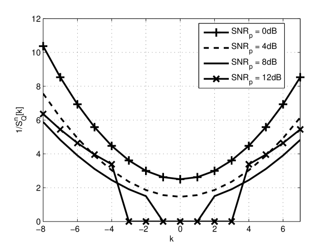
Figure 2: Inverse of the PSD of the quantization noise obtained from Algorithm 1 versus the frequency index $k$ with $C=3$ bits/sample, $F=2$, $A=0.7$, $N=100$ and $N_{p}=16$.

Fig. 2 shows the inverse of the PSD of the quantization noise $1/S_{Q^{n}_{p}}[k]$ obtained from Algorithm 1 for various values of $\textrm{SNR}_{p}$ with $C=3$ bits/sample, $N=100$, $N_{p}=16$, and $F=2$. Note that the frequency axis ranges from $-N_{p}/2$ to $N_{p}/2-1$ rather than in the interval $[0,N_{p}-1]$ for convenience of illustration. Moreover, we emphasize that $1/S_{Q^{n}_{p}}[k]$is a measure of the accuracy of quantization at frequency $k$ with $k=-N_{p}/2,...,N_{p}/2-1$, so that a larger $1/S_{Q^{n}_{p}}[k]$ implies a more refined quantization. We first observe that the optimized solution prescribes a more accurate quantization at higher frequencies, since these convey more information on the time delay, as per the CRB (13), while all frequencies contribute in equal manner to the estimate of the phase offset as per (14). Moreover, as $\textrm{SNR}_{p}$ increases, it is seen that lower frequencies tend to be neglected by the quantizer in the sense that, for such frequencies, we have $1/S_{Q^{n}_{p}}[k]=0$, and hence the signals on these frequencies are not compressed and not transmitted to the CU.

In order to validate the advantage of the proposed design, we now consider the synchronization performance under a conventional least-square joint phase and timing estimator operating on the compressed signal $\hat{Y}^{n}[k],n=0,...,F-1,k=0,...,N_{p}-1$. The estimator is given as

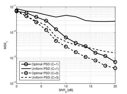
(a) $F=1$, MSE of timing offset

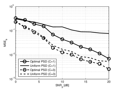
(b) $F=1$, MSE of phase offset

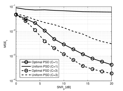
(c) $F=2$, MSE of timing offset

(d) $F=2$, MSE of phase offset

Figure 3: MSE for joint phase and timing estimation (31) versus the $\textrm{SNR}_{p}$ with $A=0.7$, $N=100$ and $N_{p}=16$.

$$(\hat{\theta},\hat{\tau})=\arg\min_{\tilde{\theta},\tilde{\tau}}\Phi(\tilde{\theta},\tilde{\tau}),$$ (31)

with $\Phi(\tilde{\theta},\tilde{\tau})=\sum_{n,k}|r^{n}_{k}-r^{n}_{k}(\tilde{\theta},\tilde{\tau})|^{2}$ where $r^{n}_{k}=\arg(\hat{Y}^{n}[k]X^{*}[k])/{2\pi}$ and $r^{n}_{k}(\tilde{\theta},\tilde{\tau})=\tilde{\theta}-k/N_{p}(n+\tilde{\tau})$. We evaluate the performance of the estimator (31) in terms of MSEs of time and phase offsets by considering the quantization noise with both the optimized PSD obtained from Algorithm 1 and a white PSD that is constant across all frequencies and is selected to satisfy the from the constraint (24b). The white-PSD compression scheme is considered as reference as it does not attempt to optimize quantization with the aim of enhancing synchronization.

Fig. 3(a) and Fig. 3(b) illustrate the MSE of the timing and phase offset estimates, respectively, as a function of $\textrm{SNR}_{p}$ for $C=1$ bits/sample and $C=3$ bits/sample with $F=1$, $A=0.7$, $N=100$, and $N_{p}=16$. In addition, we plot the MSE of the timing and phase offset estimates in case of $F=2$ in Fig. 3(c) and Fig. 3(d), respectively, under the same parameters. We observe that the proposed scheme significantly outperforms the conventional white-PSD strategy, and that the gain of the proposed scheme is more pronounced for larger SNR values. This is because as the SNR grows, the impact of the quantization noise becomes more relevant compared to the channel noise. Furthermore, a larger oversampling factor $F$ is seem to yield an improved performance only for the proposed optimization scheme and not with the conventional white-PSD scheme. This is because in the latter case, the performance benefits of a larger number of observation are offset by the increased fronthaul overhead, which leads to a more pronounced quantization noise.

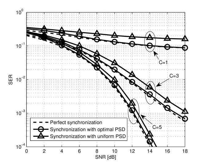
Figure 4: SER with uncoded BPSK transmission versus SNR with joint phase and timing estimation (31), $F=2$, $A=0.7$, $N=100$ and $N_{p}=16$.

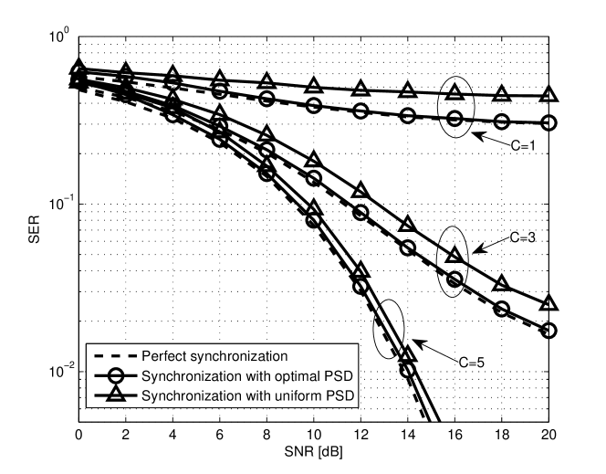
Figure 5: SER with uncoded QPSK transmission versus SNR with joint phase and timing estimation (31),$F=2$, $A=0.7$, $N=100$ and $N_{p}=16$.

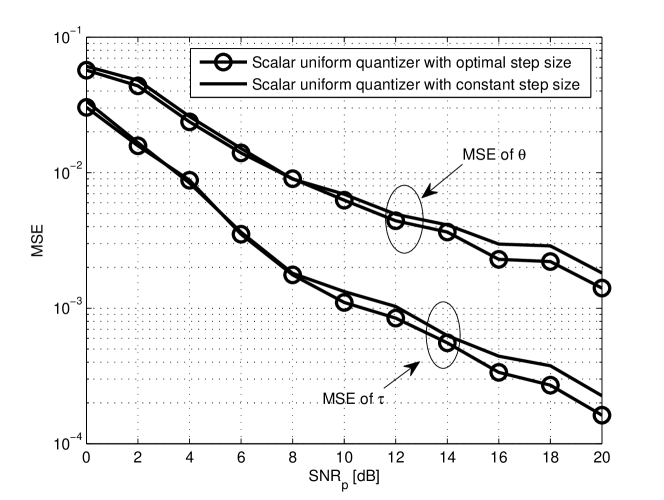
Figure 6: MSE of joint phase and timing estimation versus $\textrm{SNR}_{p}$ in the presence of scalar fronthaul quantization and joint phase and timing estimation (31) with $F=2$, $C=3$, $A=0.7$, $N=100$ and $N_{p}=16$.

Adopting the same estimator for time and phase offset, the system performance in terms of uncoded SER during the data phase is shown in Fig. 4 and Fig. 5 for BPSK and QPSK modulation, respectively, versus the SNR for both training and data fields, i.e., $\textrm{SNR}=\textrm{SNR}_{p}=\textrm{SNR}_{d}$, with $F=2$, $A=0.7$, $N=100$ and $N_{p}=16$. Simulation results with perfect synchronization are also presented for reference. We note that, consistently with the results in Fig. 5, the proposed method is observed to outperform the conventional white-PSD scheme more significantly as the SNR increases and as the fronthaul capacity $C$ decreases. For instance, it is seen in Fig. 5 that the proposed approach has a gain of about 0.5 dB for $C=5$ bits/sample, of about 2 dB for $C=3$ bits/sample, and of about 10 dB for $C=1$ bits/sample at sufficiently large SNR.

Finally, we elaborate on the performance of actual quantization by adopting a standard scalar uniform quantizer, instead of the additive quantization model considered so far. In particular, we choose the step size $\Delta[k]$ of the quantizer used for frequency $k$ based on the optimal PSD $S_{q}[k]$ obtained from Algorithm 1 by using the relationship $S_{q}[k]=\frac{|\Delta[k]|^{2}}{12}$. This relationship is justified by fact that, at high resolution, the quantization noise is approximately uniformly distributed. As reference, we also consider the performance of a uniform quantizer in which step size is same for all frequencies $k$, i.e., $\Delta[k]=\Delta$, with the same dynamic range as for the optimized quantizer. Fig. 6 presents the MSE of the timing and phase offset estimates versus $\textrm{SNR}_{p}$ with $F=2$, $C=3$, $A=0.7$, $N=100$ and $N_{p}=16$. We observe that the proposed scheme outperforms the conventional uniform quantizer, with a gain of about 2 dB in the high SNR regime.

V Conclusions

This paper tackles the problem of optimal fronthaul compression with the aim of enhancing the effective SNR in the presence of time and phase synchronization errors at the CU. The proposed algorithm optimizes the PSD of quantization noise at the RRHs by using the Charnes-Cooper transformation and the DC approach, and is shown to outperform the conventional solution that assumes an equal quantizer at all frequencies. Numerical results validate the analysis by evaluating the performance of the proposed design under practical synchronization algorithms and with scalar quantization. An interesting direction for future research is the consideration of frequency-selective channels and of frequency synchronization.

In this Appendix, we compute the powers of the desired signal $s_{d}[m]$ and of the interference terms $z_{s}[m]$ and of $z_{isi}[m]$ as defined in Section III-B. The power of the desired signal is approximated, using (19), as

$$\textbf{E}_{\Delta\tau,x_{d}}[|s_{d}[m]|^{2}] \approx A^{2}\textbf{E}_{\Delta\tau,x_{d}}\left[|x_{d}[m]|^{2}\left(1-\frac{\eta}{T}|\Delta\tau|\right)^{2}\right]$$ (32a)

$$=A^{2}E_{x_{d}}\left(1-\frac{2\eta}{T}\textbf{E}[|\Delta\tau|]+\frac{\eta^{2}}{T^{2}}\textbf{E}[|\Delta\tau|^{2}]\right)$$ (32b)

$$=A^{2}E_{x_{d}}\left(1-\frac{\eta\Delta\tau_{\textrm{max}}}{2T}+\frac{\eta^{2}}{T^{2}}\frac{\Delta\tau_{\textrm{max}}^{2}}{12}\right)$$ (32c)

$$\approx A^{2}E_{x_{d}}\left(1-\frac{\eta\Delta\tau_{\textrm{max}}}{2T}\right)$$ (32d)

$$\approx A^{2}E_{x_{d}}\left(1-\frac{\eta}{2T}\sqrt{12\textrm{CRB}_{\tau}}\right),$$ (32e)

where in (32c) we used the assumption $\Delta\tau\sim\emph{U}[-\frac{\Delta\tau_{\textrm{max}}}{2},\frac{\Delta\tau_{\textrm{max}}}{2}]$, which implies $\textbf{E}[|\Delta\tau|]=\frac{\Delta\tau_{\textrm{max}}}{4}$ and $\textbf{E}[|\Delta\tau|^{2}]=\frac{\Delta\tau_{\textrm{max}}^{2}}{12}$; (32d) follows by removing higher-order terms in $\Delta\tau_{\textrm{max}}$ under the assumption that $\Delta\tau_{\textrm{max}}$ is small enough; and (32e) is a consequence of the approximation $\textbf{E}[\Delta\tau^{2}]=\frac{\Delta\tau_{\textrm{max}}^{2}}{12}\approx\textrm{CRB}_{\tau}$.

The power of $z_{s}[m]$ is similarly approximated, using (19), as

$$\textbf{E}_{\Delta\tau,\Delta\theta,x_{d}}[|z_{s}[m]|^{2}] \approx A^{2}\textbf{E}_{\Delta\tau,\Delta\theta,x_{d}}\left[|x_{d}[m]|^{2}|e^{-j\Delta\theta}-1|^{2}\left(1-\frac{\eta}{T}|\Delta\tau|\right)^{2}\right]$$ (33a)

$$=A^{2}E_{x_{d}}\textbf{E}_{\Delta\tau,\Delta\theta}\left[|e^{-j\Delta\theta}-1|^{2}\left(1-\frac{2\eta}{T}|\Delta\tau|+\frac{\eta^{2}}{T^{2}}|\Delta\tau|^{2}\right)\right]$$ (33b)

$$\approx A^{2}E_{x_{d}}\textrm{CRB}_{\theta}\left(1-\frac{2\eta}{T}\textbf{E}_{\Delta\tau}[|\Delta\tau|]+\frac{\eta^{2}}{T^{2}}\textbf{E}_{\Delta\tau}[|\Delta\tau|^{2}]\right)$$ (33c)

$$\approx A^{2}E_{x_{d}}\textrm{CRB}_{\theta}\left(1-\frac{\eta}{2T}\sqrt{12\textrm{CRB}_{\tau}}\right),$$ (33d)

where the approximation in (33b) follows as

$$\textbf{E}_{\Delta\theta}[|e^{-j\Delta\theta}-1|^{2}] =2-2\textbf{E}_{\Delta\theta}[\cos(\Delta\theta)]$$ (34a)

$$=2-2\left(\frac{\sin(\Delta\theta_{\textrm{max}}/2)}{\Delta\theta_{\textrm{max}}/2}\right)$$ (34b)

$$\approx 2-2\left(1-\frac{(\Delta\theta_{\textrm{max}}/2)^{2}}{3!}\right)$$ (34c)

$$=\frac{\Delta\phi^{2}}{12}$$ (34d)

$$\approx\textrm{CRB}_{\theta},$$ (34e)

where (34c) follows from the Taylor series of the sinc function up to the second order, and (34e) is a consequence of the approximation $E[\Delta\theta^{2}]=\frac{\Delta\theta_{\textrm{max}}^{2}}{12}\approx\textrm{CRB}_{\theta}$.

Finally, using (18a), the power of $z_{isi}[m]$ is approximated as

$$E_{\Delta\tau,\mathbf{\bar{x}}_{d}}[|z_{isi}[m]|^{2}] \approx\frac{A^{2}}{T^{2}}E_{\Delta\tau,\mathbf{\bar{x}}_{d}}\left[|\textbf{a}^{T}\mathbf{\bar{x}}_{d}|^{2}\Delta\tau^{2}\right]$$ (35a)

$$=\frac{A^{2}E_{x_{d}}\bar{a}}{T^{2}}E_{\Delta\tau}[\Delta\tau^{2}]$$ (35b)

$$\approx\frac{A^{2}E_{x_{d}}\bar{a}}{T^{2}}\textrm{CRB}_{\tau}.$$ (35c)

References

- [1] “C-RAN: The road towards green RAN," China Mobile Res. Inst., Beijing, China, Oct, 2011, White Paper, ver. 2.5.
- [2] A. Checko, H. L. Christiansen, Y. Yan, L. Scolari, G. Kardaras, M. S. Berger, and L. Dittmann, “Cloud RAN for mobile networks: A technology overview," IEEE Commun. Surveys and Tutorials, vol. 17, no. 1, pp. 405-426, Dec. 2012.
- [3] A. del Coso and S. Simoens, “Distributed compression for MIMO coordinated networks with a backhaul constraint," IEEE Trans. Wireless Comm., vol. 8, no. 9, pp. 4698-4709, Sep. 2009.
- [4] L. Zhou and W. Yu, “Uplink multicell processing with limited backhaul via per-base-station successive interference cancellation," IEEE Jour. Select. Areas in Comm., vol. 31, no. 10, pp. 1981-1993, Oct. 2013.
- [5] S.-H. Park, O. Simeone, O. Sahin, and S. Shamai, “Robust and efficient distributed compression for cloud radio access networks," IEEE Trans. Veh. Techn., vol. 62, no. 2, pp. 692-703, Feb. 2013.
- [6] J. Hoydis, M. Kobayashi, and M. Debbah, “Optimal channel training in uplink network MIMO systems," IEEE Trans. Sig. Proc., vol. 59, no. 6, pp. 2824-2833, Jun. 2011.
- [7] J. Kang, O. Simeone, J. Kang, and S. Shamai, “Joint signal and channel state information compression for the backhaul of uplink network MIMO systems," IEEE Trans. on Wireless Comm., vol. 13, no. 3, pp. 1555-1567, Mar. 2014.
- [8] S.-H. Park, O. Simeone, O. Sahin, and S. Shamai, “Fronthaul compression for cloud radio access networks: signal processing advances inspired by network information theory," IEEE Signal Processing Magazine, vol. 31, no. 6, pp. 69-79, Nov. 2014.
- [9] A. Charnes and W. W. Cooper, “Programming with linear fractional functionals," Naval Research Logistics Quarterly, vol. 9, issue 3-4, pp. 181-186, Dec. 1962.
- [10] R. Horst, N. V. Thoai, “DC Programming: Overview," Journal of Optimization Theory and Applications, vol. 103, no. 1, pp. 1-43, Oct. 1999.
- [11] A. El Gamal and Y. Kim, Network information theory, Cambridge University Press, 2012.
- [12] Y. Chen, Y. C. Eldar, and A. J. Goldsmith, “Shannon meets Nyquist: Capacity of sampled Gaussian channels," IEEE Trans. on Inf. Theory, vol. 69, no. 8, pp. 4889-4914, Aug. 2013.
- [13] L. Tong, G. Xu, B. Hassibi, and T. Kailath, “Blind channel identification based on second-order statistics: A frequency-domain approach," IEEE Trans. on Inf. Theory, vol. 41, no. 1, pp. 329-334, Jan. 1995.
- [14] S. Gault, W. Hachem, and P. Ciblat, “Cramer-Rao bounds for data-aided sampling clock offset and channel estimation," in Proc. IEEE ICASSP, vol. 4, pp. iv-1029-32, May 2004.
- [15] R. Zamir and M. Feder, “On lattice quantization noise," IEEE Trans. on Inf. Theory, vol. 42, no. 4, pp. 1152-1159, Jul. 1996.
- [16] R. M. Gray, Toeplitz and Circulant Matrices: A review, Now Publishers Inc, 2006.
- [17] F. Gini, R. Reggiannini, and U. Mengali, “The modified Cramer-Rao bound in vector parameter estimation," IEEE Trans. on Comm., vol. 46, no. 1, pp. 52-60, Jan. 1998.
- [18] S. Jagannathan, H. Aghajan, A. Goldsmith, “The effect of time synchronization errors on the performance of cooperative MISO systems," in Proc. IEEE GLOBECOM 2004, pp. 102-107, Nov. 2004.