Abstract

Non-geometric flux-scaling vacua provide promising starting points to realize axion monodromy inflation via the F-term scalar potential. We show that these vacua can be uplifted to Minkowski and de Sitter by adding an $\overline{{\rm D}3}$-brane or a D-term containing geometric and non-geometric fluxes. These uplifted non-supersymmetric models are analyzed with respect to their potential to realize axion monodromy inflation self-consistently. Admitting rational values of the fluxes, we construct examples with the required hierarchy of mass scales.

1 Introduction

Motivated by realizing single field F-term axion monodromy inflation [1, 2, 3], while taking closed string moduli stabilization into account, a scheme of high scale supersymmetry breaking was proposed in [4]. The inflaton was an axion receiving a (flattened) polynomial potential from a tree-level background flux, thus achieving large field inflation with an observable tensor-to-scalar ratio and an inflationary scale of the order of the GUT scale and with an inflaton mass of order $10^{13}\,{\rm GeV}$. It is worth to emphasize that, after its inception in [5, 6, 7, 8], the stringy realization of axion monodromy inflation has become an active area of research (see e.g. [9, 10] for reviews). Just to mention a few developments, in [11] the axion responsible for inflation was identified with a deformation modulus of a ${\rm D}7$-brane, whereas in [12, 13] the axion was related to the $B$-field from the NS-NS sector integrated over a non-contractible internal two cycle. In [14] non-geometric fluxes were included in the effective theory identifying the Kähler modulus with the inflaton. Other scenarios realize axion inflation in warped resolved conifolds [15], which suffers from a too small string scale for a large axion decay constant [16]. The case of chaotic inflation with axionic-like fields considering the backreaction of the heaviest moduli has been worked out in [17]. Another attempt to embed chaotic inflation is [18] where the axion was identified with either a Wilson line or the position modulus of a ${\rm D}$-brane containing the MSSM. In the framework of F-theory [19], an axion-like field serves as inflaton for natural inflation. Special points in the moduli space for which the complex structure moduli can drive axion monodromy inflation were investigated in [20].

Since for single field inflation, the inflaton should be the lightest scalar field, all the other moduli should better acquire their masses already at tree-level. For type IIB orientifold compactifications on Calabi-Yau (CY) three-folds this means in particular that all closed string moduli, namely the axio-dilaton as well as the complex structure and Kähler moduli, should be stabilized by geometric and non-geometric fluxes. Closed string moduli stabilization with solely fluxes was discussed in [4] while its application to axion inflation was further elucidated in [21].

One of the main results of [4] is that by turning on $n+1$ fluxes for $n$ moduli, the resulting F-term scalar potential admits so-called scaling type non-supersymmetric AdS minima with the desired properties. Here scaling type means that the values of the moduli in the minimum, as well as all the mass scales, are determined by ratios of products of fluxes, thus allowing for parametric control of these quantities. This is important in order to argue for the self-consistency of the moduli stabilization scheme, i.e. that eventually the moduli are stabilized in their perturbative regime and that, e.g. the moduli masses are separated from the string and Kaluza-Klein scales.

Conceptually, the induced F-term scalar potential is related to the one of $N=2$ gauged supergravity by an orientifold projection breaking $N=2$ down to $N=1$ [22]. Recently, it was explicitly shown in [23] that the same potential also arises by appropriate dimensional reduction of double field theory on a CY three-fold equipped with fluxes. In fact, it turns out that the latter also includes a D-term potential that emerges when there are abelian gauge fields present coming from the dimensional reduction of the R-R four-form on an orientifold even three-cycle of the CY [24].

It is important to note that, throughout the work [4], it was assumed that the flux-scaling AdS vacua could be uplifted to Minkowski or to de Sitter vacua, for instance by introducing an $\overline{{\rm D}3}$-brane as in the KKLT scenario [25]. As a fairly new and significant development, it has been recently pointed out that this often employed $\overline{{\rm D}3}$-brane uplift mechanism can be described within supergravity by a nilpotent superfield [26, 27, 28] and the vacua are argued to be metastable[29]. However, in [4], for one concrete example it was shown that a naive uplift of flux-scaling AdS vacua by introducing an $\overline{{\rm D}3}$-brane in a warped throat does not work. Indeed, by increasing the warp factor, the minimum got destabilized before the cosmological constant vanished. However, for string theory to provide a reliable description of inflation, it has to explain the cosmological constant in a self-consistent compactification.

In the past years, potential realizations of dS vacua in string theory have been intensively studied from different perspectives [25, 30, 31, 32, 33, 34, 35, 36, 37, 38, 39]. Both analytical and numerical approaches have been followed to construct metastable dS vacua. Moreover, as a useful guide, no-go theorems have been derived in the context of the type II [40, 41, 42, 43, 44, 45, 46, 47, 48] and heterotic [49, 50, 51] superstrings.

One of the loopholes of these no-go theorems is the restriction of the fluxes to those visible in supergravity. However, by arguments based on T-duality [52, 53] and the developments in generalized geometry and double field theory [54, 55, 56, 57, 58] it has become clear that there might also exist so-called non-geometric fluxes. For instance, the $STU$-models [59, 60, 61, 62, 63] were analyzed in much detail for realizations of dS vacua via the introduction of T- and S-dual non-geometric fluxes.

Since the question of uplifting is clearly a very important unsettled issue in the flux-scaling scenario, it is the purpose of this paper to investigate this problem more closely. First, for the $\overline{{\rm D}3}$-brane case we will find that adding the tension of this brane to the flux induced F-term potential can lead to new flux-scaling solutions that are of Minkowski/de Sitter type. Second, as mentioned above, for $h^{21}_{+}>0$ there is an additional positive semi-definite D-term contribution to the scalar potential [24, 23] that in principle could also help with increasing the cosmological constant at the minimum. We will show that this alternative also works. Let us emphasize that these are not continuous uplifts of initial AdS minima, but just new minima lying on a different branch in the landscape.

As mentioned, the motivation for moduli stabilization in the flux-scaling scheme was the stringy realization of axion monodromy inflation. Therefore, having now two possible ways of uplifting available, we also revisit the problem of realizing axion monodromy inflation. We still find that for integer quantized fluxes, it is persistently difficult to obtain all mass scales in the right order, namely

$$\begin{split}M_{\rm s}>M_{\rm KK}>M_{\rm inf}>M_{\rm mod}>H_{\rm inf}>M_{\rm\theta}\,,\end{split}$$

where $\theta$ denotes the inflaton. However, it is known that the perturbative corrections to the prepotential of the complex structure moduli lead to a redefinition of the fluxes so that some of them become rational numbers. Phenomenologically scanning over such rational values, we identify a model in which the above hierarchy is indeed fulfilled.

This paper is organized as follows: In section 2 we briefly review type IIB orientifolds on Calabi-Yau three-folds with various geometric and non-geometric fluxes turned on. In the main section 3 we present examples of uplifted flux-scaling vacua. We discuss one model with an $\overline{{\rm D}3}$-brane uplift and another with a D-term uplift. We also show that by changing the warp factor for the former example, one can interpolate between AdS and dS vacua. In section 4 we analyze the realization of axion monodromy inflation in the model with D-term-uplift.

2 The flux-scaling scenario

In this section, we first review the salient features of the moduli stabilization scheme introduced in [4]. For more details of this construction we refer the reader to the original literature.

The starting point are orientifolds of the type IIB superstring compactified on Calabi-Yau three-folds with non-vanishing (non-)geometric fluxes turned on. Such models have indeed been investigated before [64, 65, 66, 67, 68]. The orientifold projection is $\Omega_{\rm P}(-1)^{F_{L}}\sigma$ where $\sigma$ acts such that there are ${\rm O}7$- and ${\rm O}3$-planes. For vanishing fluxes, the massless spectrum comprises $h^{1,1}_{+}$ complexified Kähler moduli $T_{\alpha}$, $h^{1,1}_{-}$ purely axionic moduli $G^{a}$, $h^{2,1}_{-}$ complex structure moduli $U^{i}$ and $h^{2,1}_{+}$ abelian gauge fields $A_{j}$ resulting from the dimensional reduction of the R-R four-form $C_{4}$ on three-cycles of the CY [69]. In addition the dilaton and the R-R 0-form give the chiral axio-dilaton, defined as $S=e^{-\phi}-iC_{0}$ in our conventions.

The various fluxes appear in a twisted differential acting on $p$-forms. This differential contains the constant fluxes $H$, $F$, $Q$ and $R$, and is given by

$$\begin{split}\mathcal{D}=d-H\wedge\>-F\circ\>-Q\bullet\>-R\,\llcorner\,,\end{split}$$ (2.1)

where the operators entering in (2.1) act as

$$\begin{split}\begin{array}[]{l@{\hspace{7pt}}c@{\hspace{12pt}}lcl}H\,\wedge\hfil\hskip 7.0&:\hfil\hskip 12.0&\mbox{$p$-form}&\to&\mbox{$(p+3)$-form}\,,\\ F\,\circ\hfil\hskip 7.0&:\hfil\hskip 12.0&\mbox{$p$-form}&\to&\mbox{$(p+1)$-form}\,,\\ Q\,\bullet\hfil\hskip 7.0&:\hfil\hskip 12.0&\mbox{$p$-form}&\to&\mbox{$(p-1)$-form}\,,\\ R\,\llcorner\hfil\hskip 7.0&:\hfil\hskip 12.0&\mbox{$p$-form}&\to&\mbox{$(p-3)$-form}\,.\end{array}\end{split}$$ (2.2)

For the different forms in a CY three-fold this action can be specified by [66]

$$\begin{split}\begin{array}[]{lcl@{\hspace{1.5pt}}l@{\hspace{40pt}}lcr@{\hspace{1.5pt}}l}\mathcal{D}\alpha_{\Lambda}&=&q_{\Lambda}{}^{A}\omega_{A}\hfil\hskip&+\,f_{\Lambda\hskip 1.0ptA}\tilde{\omega}^{A}\,,\hfil\hskip 40.&\mathcal{D}\beta^{\Lambda}&=&\tilde{q}^{\Lambda\hskip 1.0ptA}\omega_{A}\hskip&+\,\tilde{f}^{\Lambda}{}_{A}\tilde{\omega}^{A}\,,\\[8.0pt] \mathcal{D}\omega_{A}&=&-\tilde{f}^{\Lambda}{}_{A}\alpha_{\Lambda}\hfil\hskip&+\,f_{\Lambda A}\beta^{\Lambda}\,,\hfil\hskip 40.&\mathcal{D}\tilde{\omega}^{A}&=&\tilde{q}^{\Lambda\hskip 1.0ptA}\alpha_{\Lambda}\hskip&-\,q_{\Lambda}{}^{A}\beta^{\Lambda}\,.\end{array}\end{split}$$ (2.3)

with $\Lambda=0,\ldots,h^{2,1}$ and $A=0,\ldots,h^{1,1}$. For the $H$- and $R$-flux we further use the conventions

$$\begin{split}\begin{array}[]{lcl@{\hspace{70pt}}lcl}f_{\Lambda\hskip 1.0pt0}&=&r_{\Lambda}\,,\hfil\hskip 70.&\tilde{f}^{\Lambda}{}_{0}&=&\tilde{r}^{\Lambda}\,,\\[5.0pt] q_{\Lambda}{}^{0}&=&h_{\Lambda}\,,\hfil\hskip 70.&\tilde{q}^{\Lambda\hskip 1.0pt0}&=&\tilde{h}^{\Lambda}\,.\end{array}\end{split}$$ (2.4)

We also define $\tilde{\omega}^{0}=1$, and $\omega_{0}=\sqrt{g}\hskip 1.0ptd^{6}x/{\mathcal{V}}_{\mathcal{M}}$, where ${\mathcal{V}}_{\mathcal{M}}=\int_{\mathcal{M}}\sqrt{g}\hskip 1.0ptd^{6}x$ is the volume of the CY three-fold ${\mathcal{M}}$.

Imposing the nilpotency condition of the form $\mathcal{D}^{2}=0$ leads to Bianchi identities for the fluxes. In this way we obtain

$$\begin{split}\begin{array}[]{lcl@{\hspace{50pt}}lcl}0&=&\tilde{q}^{\Lambda\hskip 1.0ptA}\tilde{f}^{\Sigma}{}_{A}-\tilde{f}^{\Lambda}{}_{A}\tilde{q}^{\Sigma\hskip 1.0ptA}\,,\hfil\hskip 50.&0&=&q_{\Lambda}{}^{A}f_{\Sigma\hskip 1.0ptA}-f_{\Lambda\hskip 1.0ptA}q_{\Sigma}{}^{A}\,,\\[7.0pt] 0&=&q_{\Lambda}{}^{A}\tilde{f}^{\Sigma}{}_{A}-f_{\Lambda\hskip 1.0ptA}\tilde{q}^{\Sigma\hskip 1.0ptA}\,,\hfil\hskip 50.&0&=&\tilde{f}^{\Lambda}{}_{A}q_{\Lambda}{}^{B}-f_{\Lambda\hskip 1.0ptA}\tilde{q}^{\Lambda\hskip 1.0ptB}\,.\\[7.0pt] 0&=&\tilde{f}^{\Lambda}{}_{A}f_{\Lambda\hskip 1.0ptB}-f_{\Lambda\hskip 1.0ptA}\tilde{f}^{\Lambda}{}_{B}\,,\hfil\hskip 50.&0&=&\tilde{q}^{\Lambda\hskip 1.0ptA}q_{\Lambda}{}^{B}-q_{\Lambda}{}^{A}\tilde{q}^{\Lambda\hskip 1.0ptB}\,.\end{array}\end{split}$$ (2.5)

Implementing the orientifold projection, the invariant fluxes are

$$\begin{split}\begin{array}[]{l@{\hspace{6pt}}c@{\hspace{18pt}}llll}{\mathfrak{F}}\hfil\hskip 6.0&:\hfil\hskip 18.0&&&{\mathfrak{f}}_{\lambda}\,,&\tilde{\mathfrak{f}}^{\lambda}\,,\\ H\hfil\hskip 6.0&:\hfil\hskip 18.0&&&h_{\lambda}\,,&\tilde{h}^{\lambda}\,,\\ F\hfil\hskip 6.0&:\hfil\hskip 18.0&f_{\hat{\lambda}\,\alpha}\,,&\tilde{f}^{\hat{\lambda}}{}_{\alpha}\,,&f_{\lambda\,a}\,,&\tilde{f}^{\lambda}{}_{a}\,,\\ Q\hfil\hskip 6.0&:\hfil\hskip 18.0&q_{\hat{\lambda}}{}^{a}\,,&\tilde{q}^{\hat{\lambda}\,a}\,,&q_{\lambda}{}^{\alpha}\,,&\tilde{q}^{\lambda\,\alpha}\,,\\ R\hfil\hskip 6.0&:\hfil\hskip 18.0&r_{\hat{\lambda}}\,,&\tilde{r}^{\hat{\lambda}}\,.\end{array}\end{split}$$ (2.6)

where $\lambda=0,\ldots,h^{21}_{-}$, $\hat{\lambda}=1,\ldots,h^{21}_{+}$, $\alpha=1,\ldots,h_{+}^{1,1}$ and $a=1,\ldots,h_{-}^{1,1}$. Note that in [4], the construction was restricted to the case $h^{21}_{+}=0$, whereas here we also consider $h^{21}_{+}>0$. In fact, as shown in [23], the fluxes with index $\lambda$ contribute to an F-term scalar potential whereas the fluxes with index $\hat{\lambda}$ contribute to a positive definite D-term potential.

For moduli stabilization, we allow all orientifold even fluxes, only subject to the Bianchi identities. The superpotential generating the F-term potential takes the form [65, 66]

$$\begin{split}W=\int_{\mathcal{M}}\Bigl{[}\,\mathfrak{F}+\mathcal{D}\hskip 1.0pt\Phi^{\rm ev}_{\rm c}\Bigr{]}_{3}\wedge\Omega\,\end{split}$$ (2.7)

with the complex multiform $\Phi^{\rm ev}_{\rm c}=i\hskip 1.0ptS-i\hskip 1.0ptG^{a}\omega_{a}-i\hskip 1.0ptT_{\alpha}\hskip 1.0pt\tilde{\omega}^{\alpha}$. Using (2.3) the superpotential can be further evaluated as

$$\begin{split}W=&-\bigl{(}{\mathfrak{f}}_{\lambda}X^{\lambda}-\tilde{\mathfrak{f}}^{\lambda}F_{\lambda}\bigr{)}+i\hskip 1.0ptS\big{(}h_{\lambda}X^{\lambda}-\tilde{h}^{\lambda}F_{\lambda}\bigr{)}\\[4.0pt] &+i\hskip 1.0ptG^{a}\bigl{(}f_{\lambda}{}_{a}X^{\lambda}-\tilde{f}^{\lambda}{}_{a}F_{\lambda}\bigr{)}-i\hskip 1.0ptT_{\alpha}\bigl{(}q_{\lambda}{}^{\alpha}X^{\lambda}-\tilde{q}^{\lambda}{}^{\alpha}F_{\lambda}\bigr{)}\,.\end{split}$$ (2.8)

where the periods $X^{\lambda},F_{\lambda}$ of the holomorphic 3-form $\Omega$ are computed from the tree-level cubic prepotential ${F}={1\over 6}d_{ijk}X^{i}X^{j}X^{k}/X^{0}$ of the CY three-fold. Specifically, $\Omega$ has the expansion $\Omega=X^{\lambda}\alpha_{\lambda}-F_{\lambda}\beta^{\lambda}$.

The tree-level Kähler potential in the large complex structure limit can be expressed as [69]

$$\begin{split}K=-\log\left(-i\int_{\mathcal{M}}\Omega\wedge\overline{\Omega}\right)-\log\bigl{(}S+\overline{S}\bigr{)}-2\log{\cal V}\,.\end{split}$$ (2.9)

Here ${\mathcal{V}}=\frac{1}{6}\kappa_{\alpha\beta\gamma}t^{\alpha}t^{\beta}t^{\gamma}$ denotes the volume of the CY three-fold in Einstein frame. For future reference we also record the expansions of the Kähler and NS-NS 2-forms, respectively $J=e^{\phi/2}t^{\alpha}\omega_{\alpha}$ and $B_{2}=b^{a}\omega_{a}$.

In [23], it was explicitly shown that the F-term scalar potential

$$\begin{split}V_{F}=\frac{M_{\text{Pl}}^{4}}{4\pi}\,\,e^{K}\Bigl{(}K^{I\overline{J}}D_{I}WD_{\overline{J}}\overline{W}-3\hskip 1.0pt\bigl{|}W\bigr{|}^{2}\Bigr{)}\,,\end{split}$$ (2.10)

resulting from the Kähler potential and superpotential reviewed above, is related to the one obtained via dimensional reduction of double field theory on a Calabi-Yau three-fold with (non-)geometric fluxes. Moreover, the potential is related to $N=2$ gauged supergravity [22]. More concretely, taking the orientifold projection the latter scalar potential splits into three pieces

$$\begin{split}V=V_{F}+V_{D}+V^{\rm NS}_{\rm tad}\end{split}$$ (2.11)

where $V_{F}$ is precisely the F-term scalar potential (2.10). $V^{\rm NS}_{\rm tad}$ is the NS-NS tadpole that will be cancelled against the tension of the branes and orientifold planes, once R-R tadpole cancellation is taken into account. $V_{D}$ is an additional D-term potential

$$\begin{split}V_{D}&=-\frac{M^{4}_{\rm Pl}}{2}\,\Bigl{[}({\rm Im}\,\mathcal{N})^{-1}\Bigr{]}^{\hat{\lambda}\hat{\sigma}}\hskip 1.0ptD_{\hat{\lambda}}\hskip 1.0ptD_{\hat{\sigma}}\\[4.0pt] \end{split}$$ (2.12)

that results from the abelian gauge fields for $h^{2,1}_{+}>0$. Adjusting the results in [23] to the present conventions, the D-terms $D_{\hat{\lambda}}$ in Einstein frame are given by

$$\begin{split}D_{\hat{\lambda}}=\frac{1}{{\mathcal{V}}}\left[-r_{\hat{\lambda}}\,\big{(}e^{\phi}{\cal V}-\tfrac{1}{2}\hskip 1.0pt\kappa_{\alpha ab}\hskip 1.0ptt^{\alpha}b^{a}b^{b}\Big{)}-q_{\hat{\lambda}}{}^{a}\,\kappa_{a\alpha b}\hskip 1.0ptt^{\alpha}b^{b}+f_{{\hat{\lambda}}\alpha}\,t^{\alpha}\right].\end{split}$$ (2.13)

We have set $\tilde{r}^{{\hat{\lambda}}}=\tilde{q}^{{\hat{\lambda}}a}=\tilde{f}^{{\hat{\lambda}}}{}_{\alpha}=0$.

In [4], assuming $h^{21}_{+}=0$, the F-term scalar potential $V_{F}$ was investigated in detail, and particular attention was paid to so-called scaling type minima, in which $W$ contained only $n+1$ terms for a model with $n$ superfields. This ansatz led to solutions where the fixed moduli, as well as the resulting moduli mass scales, could be expressed as simple quotients of fluxes. This allowed to gain parametric control over certain mass scales which was important for the realization of F-term axion monodromy inflation. All scaling vacua of this type were stable non-supersymmetric AdS minima, for which the existence of an uplift to Minkowski/de Sitter was just assumed. However, for a simple concrete model it was shown that a simple uplift à la KKLT does not really work, as the additional $\overline{{\rm D}3}$-brane contribution to the scalar potential destabilized the vacuum. In the following section, we will show that for concrete simple examples Minkowski/de Sitter minima exist featuring also the nice scaling type behavior.

Non-geometric S-dual $P$-form fluxes

After adding the non-geometric $Q$-fluxes, the superpotential (2.8) is no longer covariant under S-duality transformations. It has been proposed that this covariance can be restored by including non-geometric $P$-fluxes, which transform together with the $Q$-fluxes as a doublet of the $SL(2,\mathbb{Z})$ duality group [70]. Similar to the $Q$-flux, the $P$-flux is defined as a map

$$\begin{split}P\bullet\;:\;p{\rm-form}\rightarrow(p-1){\rm-form}\,,\end{split}$$ (2.14)

and the action of $P$ on the symplectic basis is specified by

$$\begin{split}\begin{array}[]{lcl@{\hspace{70pt}}lcl}-P\bullet\alpha_{\Lambda}&=&p_{\Lambda}^{A}\,,\hfil\hskip 70.&-P\bullet\beta^{\Lambda}&=&\tilde{p}^{\Lambda A}\omega_{A}\,,\\[5.0pt] -P\bullet\omega_{A}&=&0\,,\hfil\hskip 70.&-P\bullet\tilde{\omega}^{A}&=&-p^{\Lambda A}\alpha_{\Lambda}+p_{\Lambda}^{A}\beta^{\Lambda}\,.\\ \end{array}\end{split}$$ (2.15)

The extended superpotential is derived requiring that it transforms properly under S-duality. Taking also into account the geometric moduli $G^{a}$ it is given by [4]

$$\begin{split}W^{\prime}=\int_{\mathcal{M}}\big{[}\mathfrak{F}+\mathcal{D}\Phi_{\rm c}^{\rm ev}+T_{\alpha}S\left(P\bullet\tilde{\omega}^{\alpha}\right)+\frac{1}{2}\kappa_{\alpha bc}G^{b}G^{c}\left(P\bullet\tilde{\omega}^{\alpha}\right)\big{]}_{3}\wedge\Omega_{3}\,,\end{split}$$ (2.16)

which after integrations yields

$$\begin{split}W^{\prime}=W+\left(ST_{\alpha}+\frac{1}{2}\kappa_{\alpha bc}G^{b}G^{c}\right)\left(p_{\lambda}^{\alpha}X^{\lambda}-\tilde{p}^{\lambda\alpha}F_{\lambda}\right)\,,\end{split}$$ (2.17)

where $W$ is shown in (2.8).

In this paper we will restrict attention to examples with $h^{1,1}_{-}=0$ so that the geometric $G^{a}$ moduli contribution to the scalar potential is absent. The Bianchi identities in this case were discussed in [70]. For our purposes we can take a pragmatic approach and notice that in general the only non-trivial constraint with NS-NS and $Q$-fluxes comes from the last equation of (2.5) and is just

$$\begin{split}\tilde{q}^{\Lambda A}\,h_{\Lambda}-q_{\Lambda}^{A}\,\tilde{h}^{\Lambda}=0\,.\end{split}$$ (2.18)

Performing an S-duality transformation then leads to the generalized Bianchi identity

$$\begin{split}\tilde{p}^{\Lambda A}\,\mathfrak{f}_{\Lambda}-p_{\Lambda}^{A}\,\tilde{\mathfrak{f}}^{\Lambda}=0\,.\end{split}$$ (2.19)

Here we have used that both $(P,Q)$ and $(\mathfrak{F},H)$ fluxes transform as an $SL(2,\mathbb{Z})$ doublet.

Mass Scales

Before turning to the uplift analysis in the next sections let us state our conventions and notation for the different mass scales. For the Planck mass we take $M_{\rm Pl}\sim 2.435\cdot 10^{18}$ GeV, and for the string mass $M_{\rm s}=(\alpha^{\prime})^{1/2}$. In terms of $M_{\rm Pl}$, the string and Kaluza-Klein scales are given by

$$\begin{split}M_{\rm s}=\frac{\sqrt{\pi}M_{\rm{Pl}}}{s^{\frac{1}{4}}\mathcal{V}^{\frac{1}{2}}},\quad M_{\rm KK}=\frac{M_{\rm Pl}}{\sqrt{4\pi}\mathcal{V}^{\frac{1}{4}}}\,,\end{split}$$ (2.20)

where $s=e^{-\phi}$ and $\mathcal{V}$ is the volume of the Calabi-Yau manifold in Einstein frame in string units. The moduli masses are determined by the eigenvalues of the canonically normalized mass matrix, which is defined as

$$\begin{split}(M^{2})^{i}_{j}=K^{ik}V_{kj}\,,\end{split}$$ (2.21)

where $V_{ij}=\frac{1}{2}\partial_{i}\partial_{j}V$. Finally, the gravitino mass reads

$$\begin{split}M_{3/2}^{2}=e^{K_{0}}|W_{0}|^{2}\frac{M_{\rm Pl}^{2}}{4\pi}\end{split}$$ (2.22)

where $K_{0}$ and $W_{0}$ stand for the Kähler and superpotential evaluated at the minima.

3 Uplifting to de Sitter

In this section we investigate whether, by adding additional positive definite contributions to the F-term scalar potential, one can directly find scaling type, non-supersymmetric metastable minima that are of de Sitter or Minkowski type.

Recall that in the KKLT [25] or LARGE volume scenario [71, 72], one starts with an AdS minimum and adds the contributions of an $\overline{{\rm D}3}$-brane in a warped throat. By varying the coefficient of this contribution, i.e. the warp factor, one can continuously shift the cosmological constant in the minimum from the negative AdS value to positive dS values. In the first part of this section we analyze (in a concrete example) the effect of adding an $\overline{{\rm D}3}$-brane to the F-term flux-induced potential.

In (2.11) we have recalled that for $h^{2,1}_{+}>0$ the scalar potential receives an additional positive definite D-term contribution (2.12). Thus, it is tempting to try to uplift an AdS minimum by also turning on the fluxes contributing to this D-term. We will analyze this question in the second part of this section.

3.1 Uplift via $\overline{{\rm D}3}$-brane

The common mechanism to uplift AdS vacua preserving stability is to introduce an $\overline{{\rm D}3}$-brane at a warped throat [25, 73]. This generates a contribution to the scalar potential of the form

$$\begin{split}V_{\rm up}=\frac{A}{\mathcal{V}^{4\over 3}}\,{M^{4}_{\rm Pl}\over 4\pi}\,,\end{split}$$ (3.1)

with $A$ a positive constant depending on the warp factor in the throat. Let us now consider a concrete example showing what will happen with a scaling type minimum after including the $\overline{{\rm D}3}$-brane contribution to the scalar potential.

A stable AdS minimum

Consider a CY manifold with $h^{11}_{+}=1$, $h^{11}_{-}=0$, $h^{21}_{-}=1$ and $h^{21}_{+}=0$. Therefore, the total scalar potential after tadpole cancellation is given just by the F-term. The tree-level Kähler potential reads

$$\begin{split}K=-\log(S+\overline{S})-3\log(T+\overline{T})-3\log(U+\overline{U})\,,\end{split}$$ (3.2)

and the defining superpotential is given by

$$\begin{split}W=-ifU+ih_{0}S-3ihSU^{2}-iqT\,.\end{split}$$ (3.3)

According to (2.8), $\mathfrak{f}_{1}=f$, $\tilde{h}^{1}=-h$ and $q_{0}{}^{1}=q$. In the following we will also denote $S=s+ic$, $T=\tau+i\rho$ and $U=v+iu$.

In absence of the $\overline{{\rm D}3}$-brane there is a completely stable supersymmetric AdS vacuum of scaling type. The axionic moduli are fixed at $\rho=c=u=0$ , whereas the saxions are fixed at

$$\begin{split}s=-\frac{5^{1/2}}{4}\frac{f}{\left(hh_{0}\right)^{1/2}}\,,\quad v=\frac{5^{1/2}}{3}\left(\frac{h_{0}}{h}\right)^{1/2},\quad\tau=-\frac{5^{1/2}f}{2q}\left(\frac{h_{0}}{h}\right)^{1/2}\,.\end{split}$$ (3.4)

To be in the physical regime we choose fluxes such that

$$\begin{split}f<0\,,\qquad h_{0}>0\,,\qquad h>0\,,\qquad q>0\,.\end{split}$$ (3.5)

To stay consistently in the perturbative regime, one can choose $|f|\gg 1$ and all other fluxes ${\mathcal{O}}(1)$. The value of the scalar potential at the minimum is given by

$$\begin{split}V_{0}=-\frac{9}{5^{5/2}\,4}\frac{q^{3}h^{5/2}}{f^{2}h_{0}^{3/2}}\,\frac{M_{\rm Pl}^{4}}{4\pi}\,.\end{split}$$ (3.6)

The normalized moduli masses are found to be

$$\begin{split}M^{2}_{\rm mod}=\mu_{i}\frac{q^{3}h^{5/2}}{f^{2}h_{0}^{3/2}}\,\frac{M_{\rm Pl}^{2}}{4\pi}\,,\end{split}$$ (3.7)

with coefficients

$$\begin{split}\mu_{i}=\{0.4039,0.2414,0.1208;0.5699,0.1341,0.0442\}\,.\end{split}$$ (3.8)

The first three entries are saxionic while the last three are axionic. Thus, the lightest state is axionic.

Uplift to a Minkowski minimum

Now, we add the uplift term in (3.1) for an $\overline{{\rm D}3}$-brane in the throat. Searching directly for a stable Minkowski minimum with the axions kept at the origin, one finds one, in which the saxions are shifted to

$$\begin{split}s=\frac{1}{3^{3/4}}\frac{f}{\left(hh_{0}\right)^{1/2}}\,,\quad v=\frac{1}{3^{1/4}}\left(\frac{h_{0}}{h}\right)^{1/2},\quad\tau=\frac{f}{3^{1/4}q}\left(\frac{h_{0}}{h}\right)^{1/2}\,.\end{split}$$ (3.9)

The warp dependent parameter $A$ is determined to be

$$\begin{split}A=\frac{3^{1/4}}{2}\frac{qh^{3/2}}{h_{0}^{1/2}}\,.\end{split}$$ (3.10)

Clearly to have positive saxion vacuum expectation values in the minimum, the fluxes can be chosen in the regime

$$\begin{split}f>0\,,\qquad h_{0}>0\,,\qquad h>0\,,\qquad q>0\,.\end{split}$$ (3.11)

As a consequence, one gets $A>0$, as it should be. Since the sign of $f$ is different from the supersymmetric AdS minimum, it is clear that this Minkowski vacuum is not literally a continuous uplift of the former, but constitutes a new non-supersymmetric, still scaling type, Minkowski vacuum.

After the uplift, the normalized masses have the same flux dependence (3.7) as in the AdS vacuum, though the numerical coefficients change to

$$\begin{split}\mu_{i}=\{0.8034,0.4868,0.03942;1.5559,0.2116,0.0811\}\,.\end{split}$$ (3.12)

Observe that now the lightest state is a linear combination of saxions.

Utilizing the expressions given at the end of section 2, let us compute the other relevant mass scales. The gravitino mass has the same scaling behavior as (3.7) with coefficient $\mu_{3/2}=0.3135$. Moreover, the Kaluza-Klein and string scales are given by

$$\begin{split}M_{\rm s}^{2}=\frac{3^{3/4}\pi}{2^{3/2}}\frac{q^{3/2}h}{f^{2}h_{0}^{1/2}}M_{\rm Pl}^{2},\qquad M_{\rm KK}^{2}=\frac{3^{1/2}}{16\pi}\frac{q^{2}h}{f^{2}h_{0}}M_{\rm Pl}^{2}\,\end{split}$$ (3.13)

so that the relevant ratios are determined as

$$\begin{split}\frac{M_{\rm KK}^{2}}{M_{\rm s}^{2}}=\frac{1}{2^{5/2}3^{1/4}\pi^{2}}\left(\frac{q}{h_{0}}\right)^{1/2}\!\!\!,\qquad\frac{M^{2}_{{\rm mod},i}}{M^{2}_{\rm KK}}=\frac{2^{2}\mu_{i}}{3^{1/2}}\frac{qh^{3/2}}{h_{0}^{1/2}}.\end{split}$$ (3.14)

Therefore, taking $h,q\sim{\mathcal{O}}(1)$ and $h_{0}\sim f\gg 1$ we get that parametrically the moduli are in their perturbative regime and that parametrically one can achieve the mass hierarchy $M_{\rm s}\,\begin{matrix}\gtrsim\\[-8.5359pt] {}_{p}\end{matrix}\,M_{\rm KK}\,\begin{matrix}\gtrsim\\[-8.5359pt] {}_{p}\end{matrix}\,M_{\rm mod}$, which is important for self-consistency of our approach. Notice that for $h_{0}\gg 1$ we also obtain $A\ll 1$.

Another characteristic feature of this model is that the fluxes do not contribute to the ${\rm D}7$-brane tadpole whereas

$$\begin{split}N_{{\rm D}3}=f\hskip 1.0pth\,.\end{split}$$ (3.15)

Notice that, while in the supersymmetric AdS vacuum $N_{{\rm D}3}<0$, in the Minkowski minimum $N_{{\rm D}3}>0$. Increasing $f$ clearly gives a larger flux tadpole.

This example shows that adding an $\overline{{\rm D}3}$-brane to the fluxed CY manifold the scalar potential admits new stable scaling type Minkowski vacua. Such vacua could serve as the starting point for the realization of F-term axion monodromy inflation along the lines proposed in [74, 21, 4].

Uplift to a de Sitter minimum

By choosing the parameter $A$ in the $\overline{{\rm D}3}$-brane potential larger than (3.10), one expects to also get a de Sitter vacuum. Let us analyze this in an expansion in $\Lambda=V_{0}$, i.e. the value of the scalar potential in the minimum. Indeed changing the value of $A$, in the minimum, the axions are kept at the origin while the saxions shift to

$$\begin{split}s&=\frac{1}{3^{3/4}}\frac{f}{\left(hh_{0}\right)^{1/2}}+\frac{2^{4}\cdot 7}{3^{5/2}}\frac{f^{3}h_{0}}{q^{3}h^{3}}\Lambda+\mathcal{O}(\Lambda^{2})\,,\\ v&=\frac{1}{3^{1/4}}\left(\frac{h_{0}}{h}\right)^{1/2}-\frac{2^{4}}{3^{2}}\frac{f^{2}h_{0}^{2}}{q^{3}h^{3}}\Lambda+\mathcal{O}(\Lambda^{2})\,,\\ \tau&=\frac{f}{3^{1/4}q}\left(\frac{h_{0}}{h}\right)^{1/2}+\frac{2^{4}\cdot 13}{3^{2}}\frac{f^{3}h_{0}^{2}}{q^{4}h^{3}}\Lambda+\mathcal{O}(\Lambda^{2})\,.\end{split}$$ (3.16)

The parameter $A$ is determined to be

$$\begin{split}A=\frac{3^{1/4}}{2}\frac{qh^{3/2}}{h_{0}^{1/2}}+\frac{2^{2}}{3^{1/2}}\frac{f^{2}h_{0}}{q^{2}h}\Lambda+\mathcal{O}(\Lambda^{2})\,.\end{split}$$ (3.17)

In figure 1 we display the form of the potential for a choice of parameters leading to a de Sitter minimum. Even though, for simplicity, only the dependence on a single variable (here $\tau$) is shown, the plot shows the expected behavior that is also familiar from KKLT. In particular, the dS minimum is only metastable as the potential goes to zero for large $\tau$.

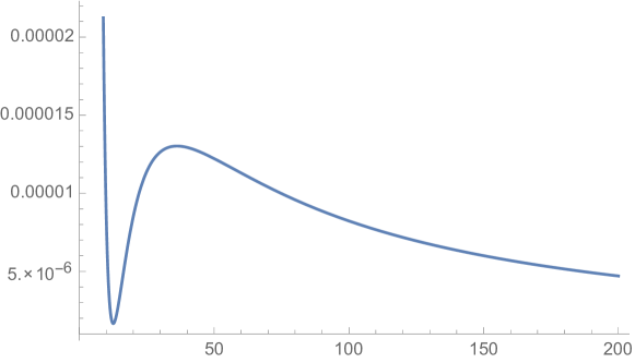
Figure 1: The scalar potential $V(\tau)$ in units of ${M_{\text{Pl}}^{4}\over 4\pi}$ for $\{s,v\}$ and the axions in their minimum. The fluxes are $h_{0}=10$, $h=q=1$, $f=5$ and $A$ is chosen to give a de Sitter minimum.

The upshot is that for small $|\Lambda|$ one can continuously interpolate from an AdS to a dS minimum. At certain critical values of $|\Lambda|$ the vevs for the saxions in (3.16) can become negative and therefore unphysical. The normalized masses also get corrected at linear order in $\Lambda$

$$\begin{split}M^{2}_{\rm mod}=\left(\mu_{i}\frac{q^{3}h^{5/2}}{f^{2}h_{0}^{3/2}}-\tilde{\mu}_{i}\Lambda+\mathcal{O}(\Lambda^{2})\right)\,\frac{M_{\rm Pl}^{2}}{4\pi}\,,\end{split}$$ (3.18)

with coefficients

$$\begin{split}\mu_{i}=\{0.8034,0.4868,0.03942;1.5559,0.2116,0.0811\}\,,\end{split}$$ (3.19)

and

$$\begin{split}\tilde{\mu}_{i}=\{46.5221,34.4038,6.1852;125.614,6.5749,3.6748\}\,.\end{split}$$ (3.20)

Note that the linear contribution of a positive cosmological constant decreases the mass of all the moduli. Thus, for too large $\Lambda$, we expect the appearance of tachyonic states. The Kaluza-Klein and string scale also receive corrections so that the relevant ratios become

$$\begin{split}\frac{M_{\rm KK}^{2}}{M_{\rm s}^{2}}&=\frac{1}{2^{5/2}3^{1/4}\pi^{2}}\left(\frac{q}{h_{0}}\right)^{1/2}-\frac{2^{3/2}}{3\pi^{2}}\frac{f^{2}h_{0}}{q^{5/2}h^{5/2}}\Lambda+\mathcal{O}(\Lambda^{2})\,,\\ \frac{M^{2}_{\rm mod,i}}{M^{2}_{\rm KK}}&=\frac{2^{2}}{3^{1/2}}\mu_{i}\frac{qh^{3/2}}{h_{0}^{1/2}}+\frac{2^{2}}{3^{3}}\left(2^{5}\cdot 13\cdot 3^{3/4}\mu_{i}+3^{5/2}\tilde{\mu}_{i}\right)\frac{f^{2}h_{0}}{q^{2}h}\Lambda+\mathcal{O}(\Lambda^{2}).\end{split}$$ (3.21)

Thus we conclude that the scaling behavior for all quantities is corrected at subleading order in $\Lambda$.

3.2 D-term uplift

In this section we investigate a second possibility for uplift, namely by taking the naturally appearing D-terms (2.12) into account. These positive semi-definite contributions do only depend on the saxionic modes and therefore do not change the axion stabilization. For concreteness, we consider a model with Hodge numbers $h^{2,1}_{+}=1$, $h^{2,1}_{-}=1$, $h^{1,1}_{+}=1$ and $h^{1,1}_{-}=0$. The derivation of the explicit form of the corresponding D-term potential is presented in some detail in Appendix A. The final result is

$$\begin{split}V_{D}=\frac{\delta}{v\tau^{2}}\left(g-\frac{r\hskip 1.0pt\tau}{3\hskip 1.0pts}\right)^{\!\!2}\,,\end{split}$$ (3.22)

where $r=f_{\hat{1}\,0}$, $g=f_{\hat{1}\,1}$, and $\delta$ is an unphysical positive constant which can be absorbed in a redefinition of the fluxes. The superpotential leading to an additional F-term potential $V_{F}$ is chosen to be

$$\begin{split}W=i\mathfrak{f}U+i\tilde{\mathfrak{f}}U^{3}-i{h}S+i{q}T\,,\end{split}$$ (3.23)

where we redefined $\mathfrak{f}_{1}=-\mathfrak{f}$, $\tilde{\mathfrak{f}}^{0}=\tilde{\mathfrak{f}}$, ${h}_{0}=-{h}$ and ${q}_{0}{}^{1}=-{q}$. After imposing the Bianchi identities (A.9), the D-term becomes

$$\begin{split}V_{D}=\frac{\delta g^{2}}{\tau^{2}v}\left(1+\frac{{q}}{3{h}}\frac{\tau}{s}\right)^{\!2}\,.\end{split}$$ (3.24)

The total scalar potential $V=V_{F}+V_{D}$, by a suitable choice of $\delta$, admits a tachyon-free (stable) Minkowski minimum with axions fixed at

$$\begin{split}Re:\Theta={q}\rho-{h}c=0,\quad u=0\,,\end{split}$$ (3.25)

and saxions at

$$\begin{split}s=\gamma_{1}\frac{{\mathfrak{f}}^{3/2}}{h\tilde{\mathfrak{f}}^{1/2}},\quad\tau=\gamma_{2}\frac{{\mathfrak{f}}^{3/2}}{{q}\tilde{\mathfrak{f}}^{1/2}},\quad v=\gamma_{3}\left(\frac{\mathfrak{f}}{\tilde{\mathfrak{f}}}\right)^{1/2}\,,\end{split}$$ (3.26)

while the constant $\delta$ is given by

$$\begin{split}\delta g^{2}=\gamma_{4}\frac{h{q}\hskip 1.0pt\tilde{\mathfrak{f}}}{{\mathfrak{f}}}\,.\end{split}$$ (3.27)

The numerical coefficients above are

$$\begin{split}\gamma_{i}=\{0.1545,1.5761,1.0318,0.0044\}\,.\end{split}$$ (3.28)

We can stay in the physical region, and have $\delta>0$, by choosing $\mathfrak{f},\tilde{\mathfrak{f}},{h},{q}>0$. The saxions are fixed in their perturbative regime for $\mathfrak{f}\gg\tilde{\mathfrak{f}}$ and $\tilde{\mathfrak{f}},h,q$ of order one. The normalized masses are given by

$$\begin{split}M_{\rm mod,i}^{2}=\mu_{i}\frac{h{q}^{3}\,\tilde{\mathfrak{f}}^{5/2}}{\mathfrak{f}^{9/2}}\frac{M_{\rm Pl}^{2}}{4\pi}\,,\end{split}$$ (3.29)

with prefactors

$$\begin{split}\mu_{i}=\{0.6986,0.0152,0.1318;0.2594,0.0524,0\}\,.\end{split}$$ (3.30)

Therefore, as expected there is one massless axion and the next lightest state is a saxion. The KK and string scales are given by

$$\begin{split}M^{2}_{\rm s}=1.428\frac{h^{1/2}\,q^{3/2}\,\tilde{\mathfrak{f}}}{\mathfrak{f}^{3}}M_{\rm Pl}^{2},\quad M^{2}_{\rm KK}=0.008\frac{{q}^{2}\,\tilde{\mathfrak{f}}}{{\mathfrak{f}}^{3}}M_{\rm Pl}^{2}\,.\end{split}$$ (3.31)

The ratio of the KK and string scale is

$$\begin{split}\frac{M^{2}_{\rm s}}{M^{2}_{\rm KK}}=178\frac{{h}^{1/2}}{{q}^{1/2}}\,,\qquad\frac{M^{2}_{\rm KK}}{M^{2}_{\rm mod}}={0.1\over\mu_{i}}{1\over hq}\frac{\mathfrak{f}^{3/2}}{\tilde{\mathfrak{f}}^{3/2}}\,.\end{split}$$ (3.32)

We can guarantee that $M_{\rm s}>M_{\rm KK}$ for $h>q$ and $M_{\rm KK}>M_{\rm mod}$ for $\mathfrak{f}\gg\tilde{\mathfrak{f}}$. Therefore, in the perturbative regime the KK scale is parametrically heavier than the moduli mass scale. Since we have in addition one massless axion, this model is a good starting point for realizing F-term axion monodromy inflation.

4 Axion monodromy inflation

In this section we study the inflaton potentials resulting from the Minkowski models obtained by including the D-term generated by non-geometric fluxes. One important difference to the analysis in [4, 21] is that now the uplift to zero or positive cosmological constant is not done by hand. Recall that to guarantee the consistency of the effective field theory approach as well as to realize a model of single field inflation, one has to stabilize the moduli such that the following hierarchy of mass scales is realized

$$\begin{split}M_{\rm s}>M_{\rm KK}>M_{\rm inf}>M_{\rm mod}>H_{\rm inf}>M_{\rm\theta}\,,\end{split}$$ (4.1)

where $H_{\rm inf}$ is the Hubble scale during inflation and $M_{\rm inf}=V^{1\over 4}_{\rm inf}$ the mass scale of inflation. Assuming a constant uplift, it was demonstrated in [4], how difficult it is to obtain such a hierarchy.

4.1 Effective field theory approach

For the model in section 3.2 with the D-term uplift, we have one unstabilized and therefore massless axion. According to [4, 21] we can try to generate a parametrically small mass for this axion by turning on additional fluxes and scale the former fluxes by a parameter $\lambda$. A good candidate for the extra flux is a $P$-flux [70] so that we now take the extended superpotential

$$\begin{split}W=\lambda W_{0}-ip\,S\,T\,U\,,\end{split}$$ (4.2)

where $W_{0}$ is given in (3.23). Note that the full set of fluxes in $W$ is not constrained by Bianchi identities. The new superpotential generates an F-term scalar potential in which the former terms scale with $\lambda^{2}$. In the large $\lambda$ limit we would like to get the old minimum. To this end we scale the D-term potential as

$$\begin{split}V_{D}=\lambda^{2}\frac{(\delta_{0}+\Delta\delta)g^{2}}{\tau^{2}v}\left(1+\frac{{q}}{3{h}}\frac{\tau}{s}\right)^{\!2}\,.\end{split}$$ (4.3)

Here we have split $\delta$ into $\delta_{0}$ given by the former value (3.27) plus a correction term $\Delta\delta$ needed to guarantee a Minkowski minimum also after including the $P$-flux.

We will assume that $\lambda$ is large and work in a $1/\lambda$ expansion. The leading order contribution to the shift in the uplift parameter turns out to be

$$\begin{split}\Delta\delta\sim-{p\,\mathfrak{f}\over\lambda\,g^{2}}\,.\end{split}$$ (4.4)

Assuming $\lambda$ sufficiently large we can also integrate out the heavy moduli and derive an effective potential for the former massless axion which is the orthogonal combination to $\Theta$ in (3.25). Since at the minimum $\Theta=0$ we can take this axion to be $\theta=c$. Integrating out the heavy moduli we obtain the effective quartic potential

$$\begin{split}V_{\rm eff}=B_{1}\,\theta^{2}+B_{2}\,\theta^{4}\end{split}$$ (4.5)

with

$$\begin{split}B_{1}\sim{\lambda\,p\,h^{2}\,q^{2}\,\tilde{\mathfrak{f}}^{5/2}\over\mathfrak{f}^{11/2}}\,,\qquad B_{2}\sim{p^{2}\,h^{3}\,q\,\tilde{\mathfrak{f}}^{5/2}\over\,\mathfrak{f}^{13/2}}\,.\end{split}$$ (4.6)

For sufficiently large $\lambda$, one can ensure that the quadratic term is dominant for say $\theta$ of ${\mathcal{O}}(10)$, as needed for large field inflation.

After canonical normalization, we can compute the mass of the inflaton. For the ratios of mass scales we find

$$\begin{split}{M^{2}_{\rm KK}\over M^{2}_{\rm mod}}\sim{\mathfrak{f}^{3/2}\over\lambda^{2}\,h\,q\,\tilde{\mathfrak{f}}^{3/2}}\,,\qquad{M^{2}_{\rm mod}\over M^{2}_{\theta}}\sim{\lambda\,h\,q\,\tilde{\mathfrak{f}}\over p\,\mathfrak{f}^{2}}\,.\end{split}$$ (4.7)

Indeed, for large $\lambda$ the inflaton mass becomes parametrically lighter than the mass of all the other moduli, which however are in danger of becoming heavier than the KK scale. Taking the product of the two mass ratios one gets

$$\begin{split}{M^{2}_{\rm KK}\over M^{2}_{\rm mod}}\,{M^{2}_{\rm mod}\over M^{2}_{\theta}}\sim{1\over\lambda\,p\,\mathfrak{f}^{1/2}\,\tilde{\mathfrak{f}}^{1/2}\,.}\end{split}$$ (4.8)

Clearly, as long as all these fluxes are positive integers and $\lambda$ large, it is in principle impossible to have both mass ratios larger than one, as desired. Note that this problem was already encountered in [4].

One potential loophole in this no-go result is the assumption that all fluxes are integer quantized. In fact, as also realized in [74], the prepotential for the complex structure moduli in the large complex structure limit is subject to perturbative and non-perturbative corrections, which take the general form (see for instance [75]) 

$$\begin{split}\widetilde{F}=F+\frac{1}{2}\hskip 1.0pta_{ij}X^{i}X^{j}+b_{i}X^{i}X^{0}+\frac{1}{2}\hskip 1.0pti\hskip 1.0pt\gamma\bigl{(}X^{0}\bigr{)}^{2}+F_{\rm inst.}\,,\end{split}$$ (4.9)

with the usual cubic term ${F}={1\over 6}d_{ijk}X^{i}X^{j}X^{k}/X^{0}$. Here, the constants $a_{ij}$ and $b_{i}$ are rational numbers, while $\gamma$ is real. From the point of view of the mirror dual threefold $\hat{M}$, they are determined as

$$\begin{split}a_{ij}&=-\frac{1}{2}\int_{\hat{M}}\hat{\omega}_{i}\wedge\hat{\omega}_{j}\wedge\hat{\omega}_{j}\,,\quad b_{i}=\frac{1}{24}\int_{M}c_{2}(\hat{M})\wedge\hat{\omega}_{i},\quad{\rm mod}\ \mathbb{Z}\\ i\,\gamma&=\frac{1}{(2\pi i)^{3}}\chi(\hat{M})\zeta(3)\,,\end{split}$$ (4.10)

with the second Chern class $c_{2}(\hat{M})$, the Euler number of the internal space $\chi(\hat{M})$ and a basis of harmonic $(1,1)$-forms $\hat{\omega}_{i}$. These constants can be smaller than one, but not arbitrarily small. Note that when evaluating the superpotential (2.8), the corrections $a_{ij}$ and $b_{i}$ can be incorporated by the following shifts in the fluxes $g_{\Lambda}\in\{\mathfrak{f}_{\Lambda},f_{\Lambda a},q_{\Lambda}{}^{\alpha}\}$

$$\begin{split}g_{0}=g_{0}-b_{i}\hskip 1.0pt\tilde{g}^{i}\,,\qquad g_{i}=g_{i}-a_{ij}\hskip 1.0pt\tilde{g}^{j}-b_{i}\hskip 1.0pt\tilde{g}^{0}\,.\end{split}$$ (4.11)

Recall that the purely imaginary contribution $i\hskip 1.0pt\gamma$ corresponds to $\alpha^{\prime}$-corrections to the Kähler potential for the Kähler moduli in a mirror-dual setting. In the large complex-structure regime we are employing here, these corrections can be neglected. Similarly, in this regime also the non-perturbative corrections $F_{\rm inst.}$ are negligible. To summarize, the polynomial corrections to the prepotential can be incorporated by a rational shift in the fluxes. This at least motivates the numerical approach to be adopted in the following section .

4.2 Numerical analysis of inflation

Instead of pursuing an effective approach, as in the previous subsection, we now follow an exact, though numerical, approach to analyze the same model. In practice we choose initial (phenomenologically motivated) values of the fluxes, compute the exact scalar potentials in terms of all moduli fields and then look numerically for stable Minkowski minima. We are particularly interested in determining whether there exists a choice of (rational) fluxes so that we can concretely realize the hierarchy of mass scales shown in (1). In figure 2 we display, for a certain choice of fluxes, the behavior of some relevant mass ratios as the scaling parameter $\lambda$ is varied.

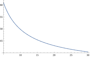
a) b)

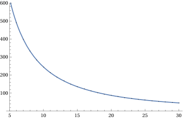
Figure 2: Ratio of relevant mass scales for a) string scale over Kaluza-Klein scale and b) the Kaluza-Klein scale over the heaviest modulus. Fluxes are chosen rational with values $h=1/220$, $\tilde{\mathfrak{f}}=1/1810$, $\mathfrak{f}=6/49$, $q=1/8$, $g=1/10$ and $p=1/10000$.

From figure 2 we conclude that for all values of $\lambda$ the KK and string mass are separated by a factor of $\mathcal{O}(10)$. Moreover, the heaviest moduli mass is lower than the KK scale by a factor of $\mathcal{O}(10^{2})$ for small $\lambda$ whereas even for values of $\lambda\sim 30$, the heaviest moduli mass is lower than the KK scale by a factor of $\mathcal{O}(10)$. Thus, we have control over these scales with hierarchy

$$\begin{split}M_{\rm Pl}>M_{\rm s}>M_{\rm KK}>M_{\rm mod}\,.\end{split}$$ (4.12)

The axions are fixed at

$$\begin{split}\Theta=\theta=u=0\,,\end{split}$$ (4.13)

whereas the saxions vary with $\lambda$ as shown in figure 3 for the same fluxes as in figure 2

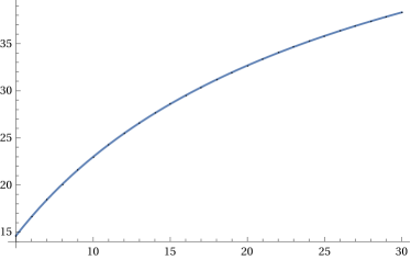
a) b)

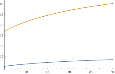
Figure 3: Vev’s of the saxionic moduli for a) $s$ and b) $\tau$ and $v$.

We observe that as $\lambda$ increases the saxionic vevs increase so that we can trust the perturbative expansion for all $\lambda$. Let us mention that for $\lambda<5$ tachyons appear in the spectrum that are not shown in figure 2. Finally, for all $\lambda$ the lightest state is related to the axion $c$ and its mass is smaller than the next heavier state by a factor of $\mathcal{O}(10^{2})$. In the following will consider $c$ as the inflaton candidate.

Next, for the values of fluxes shown above and choosing $\lambda=10$, we consider the backreaction effect [76] of the slowly rolling light axion $\theta=c$. The main task is to solve the extremum conditions $\partial_{i}V=0$ to obtain the saxions as functions of $\theta$. Due to the complexity of the scalar potential we can only perform a numerical analysis. Fixing all the heavy moduli at the minimum, the effective scalar potential turns out to be

$$\begin{split}V_{\rm eff}(\theta)\approx B_{1}\,\theta^{2}+B_{2}\,\theta^{4}\,,\end{split}$$ (4.14)

where $B\cdot 10^{14}=\{2.8711,6.8314\cdot 10^{-6}\}$. Thus, the quartic term is suppressed by a factor of $\mathcal{O}(10^{-6})$, and the effective scalar potential for sufficiently small $\theta$ has a quadratic behavior. To have a Minkowski vacuum it must be $\delta\cdot 10^{7}=6.0647$. Figure 4 shows the scalar potential including the backreaction, together with the effective scalar potential given in (4.14). From figure 4, we observe that near $c=0$ both potentials match, while the backreaction modifies the shape of the scalar potential for larger values of the inflaton $\theta$, producing a plateau-like behavior.

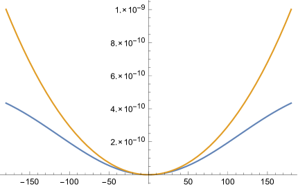
Figure 4: Backreacted (blue line) and quadratic potential in units $\frac{M_{\rm Pl}^{4}}{4\pi}$ given by eq. (4.14) for $h=1/220$, $\tilde{\mathfrak{f}}=1/1810$, $\mathfrak{f}=6/49$, $q=1/8$, $g=1/10$, $p=1/10000$ and $\lambda=10$.

In order to compute the cosmological quantities $n_{s}$, $\epsilon$, $\eta$ and $N_{e}$, we first calculate the slow-roll parameters $\epsilon$ and $\eta$ as in [21]. Recall that for the Lagrangian ${\mathcal{L}}=\frac{1}{2}f(\theta)^{2}(\partial\theta)^{2}+V(\theta)$ the slow-roll parameters are given by

$$\epsilon =\frac{1}{2f}\left(\frac{\partial V}{V}\right)^{2}\,,\qquad\eta=\frac{\partial^{2}V}{fV}-\frac{\partial f\partial V}{2f^{2}V}.$$ (4.15)

The end of inflation is determined by the point on the moduli space in which the slow-roll conditions are violated, i.e. $\epsilon\sim 1$. The starting point for the inflationary trajectory is chosen in such a way that $n_{s}=0.9667\pm 0.004$ [77]. The e-foldings as well as the tensor-to-scalar ratio are then derived from

$$\begin{split}r=16\epsilon_{*},\quad N_{e}=\int_{\theta_{\rm end}}^{\theta^{*}}d\theta\frac{fV}{\partial V}\,,\end{split}$$ (4.16)

evaluated at the pivot scale $\theta^{*}$.

The value of the amplitude of the scalar power spectrum reported experimentally is $\mathcal{P}=(2.142\pm 0.049)\cdot 10^{-9}$, and it is determined from the Hubble scale and $\epsilon$ at the pivot scale by

$$\begin{split}\mathcal{P}\sim\frac{H^{2}_{\rm inf}}{8\pi^{2}\epsilon_{*}M_{\rm Pl}^{2}}\,.\end{split}$$ (4.17)

From this expression one derives the Hubble scale during inflation. For the choice of fluxes mentioned above, we get the inflationary parameters in table 1.

Parameter	Value
$\Delta c$	$93\,M_{\rm Pl}$
$N_{e}$	$61$
$r$	$0.0980$
$n_{s}$	$0.9667$
$\mathcal{P}$	$2.14\cdot 10^{-9}$
$M_{\rm s}$	$1.04\cdot 10^{17}\,$GeV
$M_{\rm KK}$	$1.49\cdot 10^{16}\,$GeV
$M_{\rm inf}$	$4.89\cdot 10^{15}\,$GeV
$M_{\rm mod}$	$\{11.99,4.81,2.38,6.81,2.47\}\cdot 10^{14}\,$GeV
$H_{\rm inf}$	$7.82\cdot 10^{13}\,$GeV
$M_{\theta}$	$1.70\cdot 10^{13}\,$GeV

Table 1: Summary of inflationary parameters for $\lambda=10$.

Thus, for $9.44<\theta<104$ one collects $60$-efoldings for the reported spectral index $n_{s}$. From table 1 we obtain the hierarchy of mass scales

$$\begin{split}M_{\rm Pl}>M_{\rm s}>M_{\rm KK}>M_{\rm inf}>M_{\rm mod}>H_{\rm inf}>M_{\theta}\,\end{split}$$ (4.18)

with all individual scales showing the expected value. The value for the tensor-to-scalar ratio lies on the boundary of being ruled out experimentally and is a bit smaller than the value for quadratic inflation. For the same model, in Appendix B we consider a different value of $\lambda$ leading to a lower value of $r$.

This numerical example shows that by allowing rational values of the fluxes, in particular those smaller than one, it is in principle possible to freeze all moduli such that the above desired hierarchy of mass scales is realized. Of course for a concrete Calabi-Yau manifold the parameters for the polynomial terms in the prepotential (4.9) are fixed and therefore the admissible fluxes are more constrained than assumed in our phenomenological study. In particular, non-vanishing fluxes could not be smaller than $|1/24|$ and the flux $\tilde{\mathfrak{f}}$ according to (4.11) would still be an integer.

5 Conclusions

The previous work [4] proposed a scheme of high scale moduli stabilization, designed to realize axion monodromy inflation. All minima discussed there were of AdS type and thus had a negative cosmological constant. The main aim of this paper was to build more realistic models by identifying working uplift mechanisms. We considered two possible energy sources contributing a positive semi-definite term to the scalar potential, namely an $\overline{{\rm D}3}$-brane or a D-term induced by geometric and non-geometric fluxes for non-zero $h^{2,1}_{+}$. Both approaches did not uplift initial flux-scaling minima, but rather led to new de Sitter and Minkowski minima still of flux-scaling type.

We explored to what extent the uplifted models could serve as starting points for the realization of axion monodromy inflation with a parametrically controlled hierarchy of induced mass scales. As in the previous study, we found that the required hierarchy among the KK scale, the moduli mass scale and the axion mass scale was not achieved as long as we insisted on integer fluxes. Recalling that the perturbative corrections to the prepotential of the complex structure moduli effectively lead to a redefinition of the fluxes, we performed a numerical model search admitting also rational values of all fluxes. In this way we pinpointed two examples where all the desired properties could be fulfilled.

This last result should be considered as an interesting observation. Clearly, we are still far from a fully fledged string theory model. A concrete Calabi-Yau manifold with an orientifold projection has not been specified. Moreover, it has not been established conclusively that the considered vacua of four-dimensional gauged supergravity do uplift to full solutions of ten-dimensional string theory.

Acknowledgments: We would like to thank M. Fuchs and A. Guarino for valuable comments. We are specially grateful to E. Plauschinn for very useful discussions and a careful reading of appendix A. A.F. thanks the Max-Planck-Institut für Physik as well as the Ludwig-Maximillians-Universität for hospitality and support during the early stages of this work. The research of C.D. is supported by CONACyT through Assistantship No. 237801. C.D. also wants to thank the Max-Planck-Institut für Physik for its kind hospitality.

Appendix A D-term potential from $h^{2,1}_{+}$ vector multiplets

As we have seen in section 3.2, the D-term potential (2.12) can be used to uplift the cosmological constant to zero. In this appendix we will discuss the form of this D-term in some detail.

We focus on the case $h^{2,1}_{+}=1$, and $h^{2,1}_{-}=1$. To simplify we also take $h^{1,1}_{+}=1$ and $h^{1,1}_{-}=0$. In the notation of section 2 we turn on the fluxes

$$\begin{split}f_{\hat{1}\,0}=r\,,\qquad f_{\hat{1}\,1}=g\,\end{split}$$ (A.1)

whereas $\tilde{f}_{\hat{1}\,0}=0$ and $\tilde{f}_{\hat{1}\,1}=0$. The D-term potential is then given by

$$\begin{split}V_{D}=-\frac{M^{4}_{\rm Pl}}{2}\hskip 1.0pt\frac{D_{\hat{1}}^{2}}{{\rm Im}\,\mathcal{N}}\,,\end{split}$$ (A.2)

where $\mathcal{N}={\mathcal{N}}_{\hat{1}\hat{1}}$ will be determined shortly, and $D_{\hat{1}}$ reads

$$\begin{split}D_{\hat{1}}=\frac{gt}{\mathcal{V}}-re^{\phi}=\frac{3}{\tau}\left(g-\frac{r\tau}{3s}\right)\,.\end{split}$$ (A.3)

Here we have used ${\mathcal{V}}=\frac{1}{6}\kappa t^{3}$, $T+\overline{T}=\kappa t^{2}=2\tau$, and $s=e^{-\phi}$.

Let us now compute the remaining ingredient ${\rm Im}\,\mathcal{N}$. As explained in [69], when properties of the orientifold projection are taken into account, the relation between the relevant period matrix elements and the prepotential reduces to

$$\begin{split}{\mathcal{N}}_{\hat{\lambda}\hat{\sigma}}=\overline{F}_{\hat{\lambda}\hat{\sigma}}\,.\end{split}$$ (A.4)

In the right hand side the complex structure deformations associated to $h^{2,1}_{+}$ are set to zero. Working in the large complex structure limit the prepotential in our case can be expressed as

$$\begin{split}F=\frac{1}{X^{0}}\left(d_{111}X^{3}+3d_{1\hat{1}\hat{1}}XZ^{2}\right)\,,\end{split}$$ (A.5)

where $X=X^{1}$ and $Z=X^{\hat{1}}$. The form of the cubic prepotential follows imposing that under the orientifold involution $X$ and $X^{0}$ are even, whereas $Z$ is odd. The complex structure parameter associated to $h^{2,1}_{-}=1$ is defined as

$$\begin{split}U=-i\frac{X}{X^{0}}=v+iu\,.\end{split}$$ (A.6)

We then find

$$\begin{split}{\rm Im}\,\mathcal{N}=-3d_{1\hat{1}\hat{1}}\left(U+\overline{U}\right)=-6d_{1\hat{1}\hat{1}}\hskip 1.0ptv\,.\end{split}$$ (A.7)

Recall also that the Kähler potential for the complex structure sector is given by $K_{\rm cs}=-\log\left(-i\int_{\mathcal{X}}\Omega\wedge\overline{\Omega}\right)$. In our model we obtain $K_{\rm cs}=-3\log\left(U+\overline{U}\right)$, setting $X^{0}=1$ and $d_{111}=1$. Thus, in physical regime $v>0$. Now, since the D-term potential (A.2) must be positive definite, ${\rm Im}\,\mathcal{N}<0$. Therefore, $d_{1\hat{1}\hat{1}}>0$.

Substituting various preceding results in (A.2) gives the D-term potential

$$\begin{split}V_{D}=\frac{\delta}{v\tau^{2}}\left(g-\frac{r\hskip 1.0pt\tau}{3\hskip 1.0pts}\right)^{\!\!2}\,,\end{split}$$ (A.8)

where $\delta$ is a positive constant. Observe that this potential depends on all the saxions in the model. The fluxes entering in $V_{D}$ are related to the action of the twisted differential ${\mathcal{D}}$ on the even $(2,1)$ forms. Such fluxes do not enter at all in the superpotential $W$ that determines the F-term potential. However, there are Bianchi identities that mix $r_{\hat{\lambda}}$ and $f_{\hat{\lambda}\alpha}$ with NS-NS and $Q$-fluxes that might appear in $W$. In the model at hand the mixed BI constraints are

$$\begin{split}r\,\tilde{h}^{\lambda}+g\,{\tilde{q}}^{\lambda\,1}=0\,,\qquad r\,h_{\lambda}+g\,q_{\lambda}{}^{1}=0\,,\end{split}$$ (A.9)

for $\lambda=0,1$.

Appendix B A second example of axion inflation

Let us consider the same model as in section 4 but choose the limit case with $\lambda=5$. Recall that for $\lambda<5$, tachyons appears on the spectrum. As in the previous case, the lightest state is axionic and related to $\theta=c$.

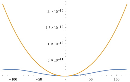
Figure 5: Backreacted (blue line) and quadratic potential in units $\frac{M_{\rm Pl}^{4}}{4\pi}$ given by eq. (4.14) for $h=1/220$, $\tilde{\mathfrak{f}}=1/1810$, $\mathfrak{f}=6/49$, $q=1/8$, $g=1/10$, $p=1/10000$ and $\lambda=5$.

For this limit situation we have, as shown in figure 2, a greater separation between the KK scale and the string scale, while the vev’s for the moduli are kept in the perturbative regime. The effective scalar potential for $\lambda=5$ has the form (4.14) with coefficients $B\cdot 10^{14}=\{1.3607,1.2675\cdot 10^{-5}\}$, so that it effectively behaves as a quadratic potential near the origin (see figure 5). In this case a Minkowski vacuum is obtained taking $\delta\cdot 10^{7}=4.2004$.

As expected, for lower values of $\lambda$ the flattening effect of the backreaction becomes more important. In table 2 we display the relevant cosmological parameters for $\lambda=5$. We find a similar pattern as in the model presented in section 4.2, but now the number of e-foldings is fairly large, while the tensor-to-scalar ratio is almost as low as for the Starobinsky model. That by decreasing $\lambda$ the model changes from quadratic to plateau-like inflation has also been observed in [21].

Parameter	Value
$\Delta c$	$86$ $M_{\rm Pl}$
$N_{e}$	$125$
$r$	$0.007$
$n_{s}$	$0.9667$
$\mathcal{P}$	$2.14\cdot 10^{-9}\,$
$M_{\rm s}$	$1.37\cdot 10^{17}\,$GeV
$M_{\rm KK}$	$1.76\cdot 10^{16}\,$GeV
$M_{\rm inf}$	$2.74\cdot 10^{15}\,$GeV
$M_{\rm mod}$	$\{7.91,3.11,1.65;6.68,2.12\}\cdot 10^{14}\,$GeV
$H_{\rm inf}$	$2.08\cdot 10^{13}\,$GeV
$M_{\theta}$	$4.69\cdot 10^{12}\,$GeV

Table 2: Summary of inflationary parameters for $\lambda=5$.

References

- [1] F. Marchesano, G. Shiu, and A. M. Uranga, “F-term Axion Monodromy Inflation,” JHEP 09 (2014) 184, 1404.3040.
- [2] A. Hebecker, S. C. Kraus, and L. T. Witkowski, “D7-Brane Chaotic Inflation,” Phys. Lett. B737 (2014) 16–22, 1404.3711.
- [3] R. Blumenhagen and E. Plauschinn, “Towards Universal Axion Inflation and Reheating in String Theory,” Phys. Lett. B736 (2014) 482–487, 1404.3542.
- [4] R. Blumenhagen, A. Font, M. Fuchs, D. Herschmann, E. Plauschinn, Y. Sekiguchi, and F. Wolf, “A Flux-Scaling Scenario for High-Scale Moduli Stabilization in String Theory,” Nucl. Phys. B897 (2015) 500–554, 1503.07634.
- [5] N. Kaloper and L. Sorbo, “A Natural Framework for Chaotic Inflation,” Phys.Rev.Lett. 102 (2009) 121301, 0811.1989.
- [6] N. Kaloper, A. Lawrence, and L. Sorbo, “An Ignoble Approach to Large Field Inflation,” JCAP 1103 (2011) 023, 1101.0026.
- [7] E. Silverstein and A. Westphal, “Monodromy in the CMB: Gravity Waves and String Inflation,” Phys.Rev. D78 (2008) 106003, 0803.3085.
- [8] L. McAllister, E. Silverstein, and A. Westphal, “Gravity Waves and Linear Inflation from Axion Monodromy,” Phys.Rev. D82 (2010) 046003, 0808.0706.
- [9] D. Baumann and L. McAllister, Inflation and String Theory. Cambridge University Press, 2015.
- [10] A. Westphal, “String cosmology ??? Large-field inflation in string theory,” Int. J. Mod. Phys. A30 (2015), no. 09, 1530024, 1409.5350.
- [11] M. Arends, A. Hebecker, K. Heimpel, S. C. Kraus, D. Lüst, C. Mayrhofer, C. Schick, and T. Weigand, “D7-Brane Moduli Space in Axion Monodromy and Fluxbrane Inflation,” Fortsch. Phys. 62 (2014) 647–702, 1405.0283.
- [12] L. McAllister, E. Silverstein, A. Westphal, and T. Wrase, “The Powers of Monodromy,” JHEP 09 (2014) 123, 1405.3652.
- [13] S. Franco, D. Galloni, A. Retolaza, and A. Uranga, “On axion monodromy inflation in warped throats,” JHEP 02 (2015) 086, 1405.7044.
- [14] F. Hassler, D. Lüst, and S. Massai, “On Inflation and de Sitter in Non-Geometric String Backgrounds,” 1405.2325.
- [15] Z. Kenton and S. Thomas, “D-brane Potentials in the Warped Resolved Conifold and Natural Inflation,” JHEP 02 (2015) 127, 1409.1221.
- [16] K. Kooner, S. Parameswaran, and I. Zavala, “Warping the Weak Gravity Conjecture,” 1509.07049.
- [17] W. Buchmüller, E. Dudas, L. Heurtier, A. Westphal, C. Wieck, and M. W. Winkler, “Challenges for Large-Field Inflation and Moduli Stabilization,” JHEP 04 (2015) 058, 1501.05812.
- [18] L. E. Ibáñez and I. Valenzuela, “The inflaton as an MSSM Higgs and open string modulus monodromy inflation,” Phys. Lett. B736 (2014) 226–230, 1404.5235.
- [19] T. W. Grimm, “Axion Inflation in F-theory,” Phys. Lett. B739 (2014) 201–208, 1404.4268.
- [20] I. García-Etxebarria, T. W. Grimm, and I. Valenzuela, “Special Points of Inflation in Flux Compactifications,” Nucl. Phys. B899 (2015) 414–443, 1412.5537.
- [21] R. Blumenhagen, A. Font, M. Fuchs, D. Herschmann, and E. Plauschinn, “Towards Axionic Starobinsky-like Inflation in String Theory,” Phys. Lett. B746 (2015) 217–222, 1503.01607.
- [22] R. D’Auria, S. Ferrara, and M. Trigiante, “On the supergravity formulation of mirror symmetry in generalized Calabi-Yau manifolds,” Nucl.Phys. B780 (2007) 28–39, hep-th/0701247.
- [23] R. Blumenhagen, A. Font, and E. Plauschinn, “Relating Double Field Theory to the Scalar Potential of N=2 Gauged Supergravity,” 1507.08059.
- [24] D. Robbins and T. Wrase, “D-terms from generalized NS-NS fluxes in type II,” JHEP 12 (2007) 058, 0709.2186.
- [25] S. Kachru, R. Kallosh, A. D. Linde, and S. P. Trivedi, “De Sitter vacua in string theory,” Phys.Rev. D68 (2003) 046005, hep-th/0301240.
- [26] R. Kallosh and T. Wrase, “Emergence of Spontaneously Broken Supersymmetry on an Anti-D3-Brane in KKLT dS Vacua,” JHEP 12 (2014) 117, 1411.1121.
- [27] E. A. Bergshoeff, K. Dasgupta, R. Kallosh, A. Van Proeyen, and T. Wrase, “ and dS,” JHEP 05 (2015) 058, 1502.07627.
- [28] R. Kallosh, F. Quevedo, and A. M. Uranga, “String Theory Realizations of the Nilpotent Goldstino,” 1507.07556.
- [29] J. Polchinski, “Brane/antibrane dynamics and KKLT stability,” 1509.05710.
- [30] A. Achucarro, B. de Carlos, J. A. Casas, and L. Doplicher, “De Sitter vacua from uplifting D-terms in effective supergravities from realistic strings,” JHEP 06 (2006) 014, hep-th/0601190.
- [31] J. Gray, Y.-H. He, A. Ilderton, and A. Lukas, “STRINGVACUA: A Mathematica Package for Studying Vacuum Configurations in String Phenomenology,” Comput. Phys. Commun. 180 (2009) 107–119, 0801.1508.
- [32] S. Krippendorf and F. Quevedo, “Metastable SUSY Breaking, de Sitter Moduli Stabilisation and Kahler Moduli Inflation,” JHEP 11 (2009) 039, 0901.0683.
- [33] U. Danielsson and G. Dibitetto, “On the distribution of stable de Sitter vacua,” JHEP 03 (2013) 018, 1212.4984.
- [34] J. Blåbäck, U. Danielsson, and G. Dibitetto, “Fully stable dS vacua from generalised fluxes,” JHEP 08 (2013) 054, 1301.7073.
- [35] C. Damian, L. R. Diaz-Barron, O. Loaiza-Brito, and M. Sabido, “Slow-Roll Inflation in Non-geometric Flux Compactification,” JHEP 06 (2013) 109, 1302.0529.
- [36] C. Damian and O. Loaiza-Brito, “More stable de Sitter vacua from S-dual nongeometric fluxes,” Phys. Rev. D88 (2013), no. 4, 046008, 1304.0792.
- [37] R. Kallosh, A. Linde, B. Vercnocke, and T. Wrase, “Analytic Classes of Metastable de Sitter Vacua,” JHEP 10 (2014) 11, 1406.4866.
- [38] M. Rummel and Y. Sumitomo, “De Sitter Vacua from a D-term Generated Racetrack Uplift,” JHEP 01 (2015) 015, 1407.7580.
- [39] J. Blåbäck, U. H. Danielsson, G. Dibitetto, and S. C. Vargas, “Universal dS vacua in STU-models,” 1505.04283.
- [40] M. P. Hertzberg, S. Kachru, W. Taylor, and M. Tegmark, “Inflationary Constraints on Type IIA String Theory,” JHEP 12 (2007) 095, 0711.2512.
- [41] S. S. Haque, G. Shiu, B. Underwood, and T. Van Riet, “Minimal simple de Sitter solutions,” Phys. Rev. D79 (2009) 086005, 0810.5328.
- [42] R. Flauger, S. Paban, D. Robbins, and T. Wrase, “Searching for slow-roll moduli inflation in massive type IIA supergravity with metric fluxes,” Phys. Rev. D79 (2009) 086011, 0812.3886.
- [43] U. H. Danielsson, S. S. Haque, G. Shiu, and T. Van Riet, “Towards Classical de Sitter Solutions in String Theory,” JHEP 09 (2009) 114, 0907.2041.
- [44] B. de Carlos, A. Guarino, and J. M. Moreno, “Flux moduli stabilisation, Supergravity algebras and no-go theorems,” JHEP 1001 (2010) 012, 0907.5580.
- [45] C. Caviezel, T. Wrase, and M. Zagermann, “Moduli Stabilization and Cosmology of Type IIB on SU(2)-Structure Orientifolds,” JHEP 04 (2010) 011, 0912.3287.
- [46] T. Wrase and M. Zagermann, “On Classical de Sitter Vacua in String Theory,” Fortsch. Phys. 58 (2010) 906–910, 1003.0029.
- [47] G. Shiu and Y. Sumitomo, “Stability Constraints on Classical de Sitter Vacua,” JHEP 09 (2011) 052, 1107.2925.
- [48] A. Borghese, D. Roest, and I. Zavala, “A Geometric bound on F-term inflation,” JHEP 09 (2012) 021, 1203.2909.
- [49] S. R. Green, E. J. Martinec, C. Quigley, and S. Sethi, “Constraints on String Cosmology,” Class. Quant. Grav. 29 (2012) 075006, 1110.0545.
- [50] F. F. Gautason, D. Junghans, and M. Zagermann, “On Cosmological Constants from alpha’-Corrections,” JHEP 06 (2012) 029, 1204.0807.
- [51] D. Kutasov, T. Maxfield, I. Melnikov, and S. Sethi, “Constraining de Sitter Space in String Theory,” Phys. Rev. Lett. 115 (2015), no. 7, 071305, 1504.00056.
- [52] J. Shelton, W. Taylor, and B. Wecht, “Nongeometric flux compactifications,” JHEP 0510 (2005) 085, hep-th/0508133.
- [53] J. Shelton, W. Taylor, and B. Wecht, “Generalized Flux Vacua,” JHEP 0702 (2007) 095, hep-th/0607015.
- [54] G. Aldazabal, D. Marqués, and C. Núñez, “Double Field Theory: A Pedagogical Review,” Class.Quant.Grav. 30 (2013) 163001, 1305.1907.
- [55] D. S. Berman and D. C. Thompson, “Duality Symmetric String and M-Theory,” Phys.Rept. 566 (2014) 1–60, 1306.2643.
- [56] D. Andriot, M. Larfors, D. Lüst, and P. Patalong, “A ten-dimensional action for non-geometric fluxes,” JHEP 09 (2011) 134, 1106.4015.
- [57] D. Geissbuhler, D. Marqués, C. Núñez, and V. Penas, “Exploring Double Field Theory,” JHEP 1306 (2013) 101, 1304.1472.
- [58] R. Blumenhagen, X. Gao, D. Herschmann, and P. Shukla, “Dimensional Oxidation of Non-geometric Fluxes in Type II Orientifolds,” JHEP 1310 (2013) 201, 1306.2761.
- [59] A. Font, A. Guarino, and J. M. Moreno, “Algebras and non-geometric flux vacua,” JHEP 12 (2008) 050, 0809.3748.
- [60] A. Guarino and G. J. Weatherill, “Non-geometric flux vacua, S-duality and algebraic geometry,” JHEP 0902 (2009) 042, 0811.2190.
- [61] B. de Carlos, A. Guarino, and J. M. Moreno, “Complete classification of Minkowski vacua in generalised flux models,” JHEP 02 (2010) 076, 0911.2876.
- [62] G. Aldazabal, D. Marqués, C. Núñez, and J. A. Rosabal, “On Type IIB moduli stabilization and N = 4, 8 supergravities,” Nucl.Phys. B849 (2011) 80–111, 1101.5954.
- [63] G. Dibitetto, A. Guarino, and D. Roest, “Charting the landscape of N=4 flux compactifications,” JHEP 1103 (2011) 137, 1102.0239.
- [64] M. Graña, J. Louis, and D. Waldram, “Hitchin functionals in N=2 supergravity,” JHEP 0601 (2006) 008, hep-th/0505264.
- [65] I. Benmachiche and T. W. Grimm, “Generalized N=1 orientifold compactifications and the Hitchin functionals,” Nucl.Phys. B748 (2006) 200–252, hep-th/0602241.
- [66] M. Graña, J. Louis, and D. Waldram, “SU(3) x SU(3) compactification and mirror duals of magnetic fluxes,” JHEP 0704 (2007) 101, hep-th/0612237.
- [67] A. Micu, E. Palti, and G. Tasinato, “Towards Minkowski Vacua in Type II String Compactifications,” JHEP 0703 (2007) 104, hep-th/0701173.
- [68] E. Palti, “Low Energy Supersymmetry from Non-Geometry,” JHEP 0710 (2007) 011, 0707.1595.
- [69] T. W. Grimm and J. Louis, “The Effective action of N = 1 Calabi-Yau orientifolds,” Nucl.Phys. B699 (2004) 387–426, hep-th/0403067.
- [70] G. Aldazabal, P. G. Camara, A. Font, and L. Ibáñez, “More dual fluxes and moduli fixing,” JHEP 0605 (2006) 070, hep-th/0602089.
- [71] V. Balasubramanian, P. Berglund, J. P. Conlon, and F. Quevedo, “Systematics of moduli stabilisation in Calabi-Yau flux compactifications,” JHEP 0503 (2005) 007, hep-th/0502058.
- [72] J. P. Conlon, F. Quevedo, and K. Suruliz, “Large-volume flux compactifications: Moduli spectrum and D3/D7 soft supersymmetry breaking,” JHEP 08 (2005) 007, hep-th/0505076.
- [73] S. Kachru, R. Kallosh, A. D. Linde, J. M. Maldacena, L. P. McAllister, and S. P. Trivedi, “Towards inflation in string theory,” JCAP 0310 (2003) 013, hep-th/0308055.
- [74] R. Blumenhagen, D. Herschmann, and E. Plauschinn, “The Challenge of Realizing F-term Axion Monodromy Inflation in String Theory,” JHEP 01 (2015) 007, 1409.7075.
- [75] S. Hosono, A. Klemm, and S. Theisen, “Lectures on mirror symmetry,” hep-th/9403096. [Lect. Notes Phys.436,235(1994)].
- [76] X. Dong, B. Horn, E. Silverstein, and A. Westphal, “Simple exercises to flatten your potential,” Phys.Rev. D84 (2011) 026011, 1011.4521.
- [77] Planck Collaboration Collaboration, P. Ade et al., “Planck 2015. XX. Constraints on inflation,” 1502.02114.