Quantifying the UV continuum slopes of galaxies to $z\sim 10$ using deep Hubble+Spitzer/IRAC observations

Abstract

Measurements of the $UV$-continuum slopes $\beta$ provide valuable information on the physical properties of galaxies forming in the early universe, probing the dust reddening, age, metal content, and even the escape fraction. While constraints on these slopes generally become more challenging at higher redshifts as the UV continuum shifts out of the Hubble Space Telescope bands (particularly at $z>7$), such a characterisation actually becomes abruptly easier for galaxies in the redshift window $z=9.5-10.5$ due to the Spitzer/IRAC 3.6$\mu$m-band probing the rest-UV continuum and the long wavelength baseline between this Spitzer band and the Hubble H_f160w band. Higher S/N constraints on $\beta$ are possible at $z\sim 10$ than at $z=8$. Here we take advantage of this opportunity and five recently discovered bright $z=9.5-10.5$ galaxies to present the first measurements of the mean $\beta$ for a multi-object sample of galaxy candidates at $z\sim 10$. We find the measured $\beta_{\rm obs}$’s of these candidates are $-2.1\pm 0.3\pm 0.2$ (random and systematic), only slightly bluer than the measured $\beta$’s ($\beta_{\rm obs}\approx-1.7$) at $3.5<z<7.5$ for galaxies of similar luminosities. Small increases in the stellar ages, metallicities, and dust content of the galaxy population from $z\sim 10$ to $z\sim 7$ could easily explain the apparent evolution in $\beta$.

1 Introduction

Thanks to extremely sensitive near-infrared (NIR) imaging obtained using Wide Field Camera 3 (WFC3) on the Hubble Space Telescope it is now possible to routinely identify galaxies  at very high redshift ($z>6$: e.g., Oesch et al. 2010; Bunker et al. 2010; Wilkins et al. 2010; Wilkins et al. 2011a; Bouwens et al. 2011b; Finkelstein et al. 2010, 2012; Oesch et al. 2012; McLure et al. 2013; Schmidt et al. 2014) with the first samples now being identified at $z\sim 10$ and beyond, less than 500 Myr after the Big Bang (Bouwens et al. 2011a; Zheng et al. 2012; Ellis et al. 2013; Oesch et al. 2013, 2014, 2015b; Zitrin et al. 2014; Ishigaki et al. 2015; Bouwens et al. 2015b).

One area of significant interest in the study of distant galaxies regards their spectral characteristics. At very early times, we might expect galaxies to potentially have very different SEDs than at latter times. In particular, one would expect galaxies to be bluer in terms of their rest-frame UV colours and UV-optical breaks, both due to a younger stellar population (Wilkins et al. 2013a) and a lower dust content (e.g., Wilkins et al. 2011b; Bouwens et al. 2009, 2012; Finkelstein et al. 2012). In fact, there has been some evidence for bluer UV colours at high redshift (Lehnert & Bremer 2003; Papovich et al. 2004; Stanway et al. 2005; Bouwens et al. 2006, 2009, 2012, 2014a; Wilkins et al. 2011b; Finkelstein et al. 2012; Kurczynski et al. 2014) though the strength of the evolution at the highest redshifts has been subject to some debate (Dunlop et al. 2012; Robertson et al. 2013). Evolution in the size of the Balmer break is less easily inferred (Stark et al. 2009; Gonzalez et al. 2010; McLure et al. 2011) largely due to the presence of strong nebular emission lines (Shim et al. 2011; Schaerer & de Barros 2010; Wilkins et al. 2013b), but now seems clear from $z\sim 6$ to $z\sim 2$ (Stark et al. 2013; Gonzalez et al. 2014; Schaerer & de Barros 2013; Labbé et al. 2013; Smit et al. 2014; Salmon et al. 2015).

The spectral characteristics of galaxies at $z\sim 8$ and $z\sim 8.5$ have also been explored (Bouwens et al. 2010, 2013; Finkelstein et al. 2010, 2012; Dunlop et al. 2013), but are more difficult to robustly quantify due to the limited leverage in wavelength available for constraining these slopes and corrections required to remove the impact of the IGM absoprtion (Bouwens et al. 2014a). This is particularly true for $UV$-continuum slope determinations at $z\sim 8.5$-9.5. Given the challenges in deriving the spectral characteristics of galaxies at $z\sim 8.5$-9.5, it may seem that further advances may need to wait until the James Webb Space Telescope (JWST).

Fortunately, as we will show, we can make immediate progress on this issue by taking advantage of the deep IRAC observations available for galaxy samples at $z\sim 10$ from the Spitzer Space Telescope. Over the redshift interval $z\sim 9.5$-10.5, the Hubble $H$-band band and the IRAC $3.6\mu$m band fall in the $UV$-continuum. The wavelength leverage is sufficient between these bands that one can plausibly quantify the UV-continuum slopes of galaxies more accurately at $z\sim 10$ than is possible at $z\sim 8$ and especially at $z\sim 8.5$-9, as we demonstrate in §2.2 of this paper.

Opportunities to use $z\sim 10$ samples to perform such studies now exist thanks to the deep near-IR data available from Hubble in the Cosmic Assembly Near-Infrared Deep Extragalactic Survey (CANDELS, Grogin et al. 2011; Koekemoer et al. 2011), Hubble Ultra-Deep Field 2009/2012 programs (Bouwens et al. 2011; Koekemoer et al. 2013; Ellis et al. 2013), and Cluster Lensing and Supernovae survey with Hubble (CLASH: Postman et al. 2012) programs. The samples range from particularly faint sources over the HUDF/XDF (Ellis et al. 2013; Oesch et al. 2013) and the Frontier Fields (Zitrin et al. 2014) to brighter sources located over CANDELS (Oesch et al. 2014) and CLASH (e.g. Zheng et al. 2012, Coe et al. 2013, and  Zitrin et al. 2014).

Particularly valuable for probing the spectral characteristics of galaxies in the early universe are those $z\sim 10$ candidates that are intrinsically bright or lensed, since those sources have sufficient S/N with IRAC that one can use them to quantify the mean $UV$-continuum slope of galaxies at very early times. To date, five such galaxies have been identified in the magnitude range 26-27 mag from the CANDELS fields (Oesch et al. 2014) and behind lensing clusters (Zheng et al. 2012).

In this paper, we make use of these 5 particularly bright $z\sim 10$ candidates to derive, for the first time, the mean $UV$-continuum slope $\beta$ at $z\sim 10$ for a multi-object sample. We compare the observed properties with predictions from recent cosmological galaxy formation simulations to provide some context. Such simulations are valuable given that the $UV$-continuum slopes and $UV$-optical colours can be affected by a complex mixture of different factors including the joint distribution of stellar masses, ages, metallicities, and the escape fraction – which makes it difficult to interpret the observations in terms of a single variable (Bouwens et al. 2010; Wilkins et al. 2011).

This paper is organised as follows: in Section 2 we describe recent observations of candidate $z\sim 10$ star forming galaxies. In Section 3 we interpret observations of these systems in the context of dust emission. Finally, in Section 4 we present our conclusions. Throughout this work magnitudes are calculated using the $AB$ system (Oke & Gunn 1983). In calculating absolute magnitudes we assume a $\Omega_{M}=0.3$, $\Omega_{\Lambda}=0.7$, $h=0.7$ cosmology.

2 Observations of the UV-continuum slope

2.1 Data and Sample Selection

This paper is based on the bright $z\sim 10$ galaxy sample selected over the GOODS fields from Oesch et al. (2014) as well the $z\sim 9.6$ CLASH source behind MACS1149 identified in Zheng et al. (2012). For details on the datasets, we refer the reader to the discovery papers. We summarise the photometry of these sources in Table 1.

In brief, the candidates from Oesch et al. (2014) were identified using the complete Hubble dataset from the CANDELS survey (Grogin et al. 2011, Koekemoer et al. 2011) in addition to ancillary Advanced Camera for Surveys (ACS) data mostly from the GOODS survey. The central area of the GOODS-South and North fields represent the CANDELS Deep survey, which reach to H${}_{f160w}=27.8$ mag ($5\sigma$), while the outer regions are covered with slightly shallower data H${}_{f160w}=27.1$ mag. Galaxy candidates at $z\sim 10$ were identified based on the spectral break shortward of Lyman-$\alpha$ resulting in a red color of $($J${}_{f125w}-$H${}_{f160w})>1.2$ and complete non-detection in all shorter wavelength filters. While Oesch et al. (2014) also selected $z\sim 9$ galaxies with a weaker continuum break, here we restrict our analysis to the redder color selection resulting in galaxies with $z_{phot}\ga 9.5$.

Here we make use of a redetermination of the IRAC photometry for the four sources in the Oesch et al. (2014) sample. For these measurements, we take advantage of new reductions of the Spitzer/IRAC 3.6 $\mu$m and 4.5 $\mu$m imaging data over the GOODS fields from Labbe et al. (2015). These reductions include all data from the original GOODS, the Spitzer Extended Deep Survey (SEDS: Ashby et al. 2013), the IRAC Ultra Deep Field (IUDF: Labbé et al. 2015), and S-CANDELS (Ashby et al. 2015) programs. The average 5$\sigma$ depths of the IRAC data within 1″ radius apertures are 27.0 and 26.7 mag in the two channels, respectively.

Our measurements again make use of the mophongo software (Labbé et al. 2006, 2010, 2013) to model and subtract the flux from neighboring sources, but include significantly improved PSF modeling. Our derived PSFs account for the orientation of all exposures that contribute to our IRAC reductions. Our rederived IRAC fluxes are completely consistent within the errors with those given in Oesch et al. (2014). Three of the four $z\sim 10$ galaxy candidates from Oesch et al. (2014) are significantly detected ($>4.5\sigma$) in these data in at least one filter. In particular, the brightest source GN-z10-1 with a photometric redshift of $z_{phot}=10.2\pm 0.4$ is robustly detected in the 3.6 $\mu$m channel at $\sim 7\sigma$, allowing for an individual estimate a UV-continuum slope for this source.

Equally important for robust measurements of the $H_{160}-[3.6]$ colors are accurate measurements of the total $H_{160}$-band flux. Our determination of the total $H_{160}$-band flux is as described in Oesch et al. (2014) and includes all the light inside an elliptical aperture extending to 2.5 Kron (1980) radii. The measured flux inside the utilized Kron aperture is corrected to total (typically a $\sim$0.2 mag correction) based on the expected light outside this aperture (Dressel et al. 2012).

As a correction to total is performed for both the HST $H_{160}$-band photometry and for the Spitzer/IRAC photometry, colors derived from HST to Spitzer/IRAC should not suffer from significant biases. Nevertheless, it was worthwhile to verify that this was the case by applying the HST-to-Spitzer PSF-correction kernel to the HST data (derived from mophongo) and then measuring total magnitudes from the HST data in the same way as the Spitzer/IRAC data. Given the relatively small number of $z\sim 10$ candidates in our sample and their limited S/N after convolving with the IRAC PSF correction kernel, we perform this test on a sample of bright ($H_{160,AB}<25$) $z\sim 4$ galaxies from the Bouwens et al. (2015a) catalogs. We found that the total magnitudes we recover by applying this procedure to the HST observations of these $z\sim 4$ sources were consistent to $<0.1$ mag in the median with that derived using our primary method.

To probe intrinsically fainter galaxies while maintaining a sufficiently high signal-to-noise, we can take advantage of sources which are lensed by foreground galaxies (or clusters of galaxies). Several $z\sim 10$ candidates have now been discovered in cluster searches (Zheng et al. 2012; Coe et al. 2013; Zitrin et al. 2014), with more likely to be identified in the near future as a result of the ongoing Hubble Frontier Fields observations.

Of the three currently known $z\sim 10$ candidates we concentrate on MACS1149-JD (Zheng et al. 2012). The object presented by Zitrin et al. (2014) does not currently have sufficiently deep IRAC imaging to provide anything other than a weak upper limit on the rest-frame UV-continuum slope. The object presented by Coe et al. (2013) has a photometric redshift of $z\sim 10.7$, at which redshift the $H_{160}$-band flux could be affected by the position of the Lyman-$\alpha$ break within the $H_{160}$ band and/or Lyman-$\alpha$ line emission.

MACS1149-JD was identified in a search of 12 CLASH clusters and has strong detections in both the JH_f140w and H_f160w bands with weaker detections in both Y_f105w and J_f125w and non-detections in several optical bands. Photometric redshift fitting of the sources photometry suggests it is $z\sim 9.6$. Zheng et al. (2012) presented Spitzer/IRAC photometry of MACS1149-JD ([3.6]$<160\,{\rm nJy},\,1\sigma$) based on observations taken under Program ID 60034 (PI: Egami). We augment these observations with Frontier Fields observations and archival data taken as part of the Spitzer UltRa Faint SUrvey Program (Surfs’Up, Bradač et al. 2014) and measure a [3.6] flux of $175\pm 44$ nJy (see Bouwens et al. 2014b). This is consistent with that reported by both Zheng et al. (2012) ($<160\,{\rm nJy},\,1\sigma$) and Bradač et al. (2014) ($190\pm 87\,{\rm nJy}$).

Table 1: Photometry and derived properties for the $z\sim 10$ sources, and the bright stack, considered in this work.

	$z$	$M_{1500}$	Hf160w/nJy	[3.6]/nJy	H${}_{f160w}-$[3.6]	$\beta_{\rm obs}$	$A_{1500,{\rm C00}}$	$A_{1500,{\rm SMC}}$
							(assumes $\beta_{\rm int}=-2.54$)7
GN-z10-11,2	$10.2$	$-21.6$	$152\pm 10$	$136\pm 29$	$-0.1\pm 0.2$	$-2.1\pm 0.3$	$0.9\pm 0.6$	$0.5\pm 0.3$
GN-z10-21,2	$9.8$	$-20.7$	$68\pm 9$	$45\pm 26$	$-0.5\pm 0.6$	$-2.5\pm 0.7$	$0.1\pm 1.6$	$0.1\pm 0.9$
GN-z10-31,2	$9.5$	$-20.6$	$73\pm 8$	$59\pm 24$	$-0.2\pm 0.5$	$-2.3\pm 0.5$	$0.6\pm 1.1$	$0.3\pm 0.6$
GS-z10-11,2	$9.9$	$-20.6$	$66\pm 9$	$71\pm 27$	$0.1\pm 0.4$	$-1.9\pm 0.5$	$1.4\pm 1.1$	$0.8\pm 0.6$
MACS1149-JD14	$9.6$	$-19.4$4	$190\pm 13.3$5	$177\pm 44$	$-0.1\pm 0.3$	$-2.1\pm 0.3$	$1.0\pm 0.7$	$0.6\pm 0.4$
STACK	-	-	-	-	$-0.1\pm 0.2$6	$-2.1\pm 0.3$6	$0.9\pm 0.6$	$0.5\pm 0.3$

¹ Oesch et al. (2014). ² included in stack. ³ Zheng et al. (2012), Bouwens et al. (2014b). ⁴ MACS1149-JD is gravitationally lensed by a foreground cluster, we determine the un-lensed absolute magnitude using the best-fit magnification of $14.5$. ⁵ We independently measure the [3.6] flux for MACS1149-JD using the Frontier Fields Spitzer/IRAC observations combined with observations taken as part of the Spitzer UltRa Faint SUrvey Program (SURFSUP, Bradač et al. 2014) and Program ID 60034 (PI: Egami). Our flux measurements are consistent with those reported by both Zheng et al. (2012) ($<160\,{\rm nJy},\,1\sigma$) and Bradač et al. (2014) ($190\pm 87\,{\rm nJy}$). ⁶ The uncertainty on the mean increases to $\pm 0.3$, if we assume there is significant intrinsic scatter in the $\beta$ distribution as observed at $z\sim 4$-5 (Bouwens et al. 2009, 2012; Castellano et al. 2012; Rogers et al. 2014: see §2.2). ⁷ The intrinsic $UV$-continuum slope predicted in dynamical simulation at $z\sim 10$ assuming $f_{\rm esc}=0$ (§3).

2.1.1 Bright Stack

The uncertainties on the $UV$-continuum slopes of individual sources is large enough that it is useful to consider constraints for the average $z\sim 10$ source from the Oesch et al. (2014) bright sample. We therefore stack the photometry of the 4 $z\sim 10$ candidates presented in Oesch et al. (2014). The H${}_{f160w}-$[3.6] colour of the stack is $-0.1\pm 0.2$. If we stack only GN-z10-1 and GN-z10-2 (i.e. excluding sources without JH_f140w detections) we find H${}_{f160w}-$[3.6]$=-0.2\pm 0.2$.

2.2 Measuring the UV continuum slope

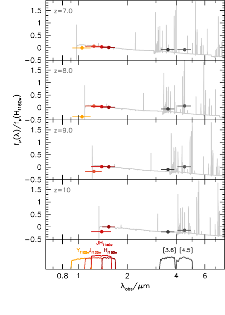
Figure 1: Relative observed near-IR photometry of a model star-forming galaxy at $z\in\{7,8,9,10\}$ highlighting the bands available to measure the rest-frame UV-continuum slope. At $z>9.6$, the Spitzer/IRAC [3.6] band can be combined with the H_f160w band to measure the UV continuum slope over a large wavelength baseline, minimising its uncertainty. At $z\sim 8$ only the JH_f140w and H_f160w bands are uncontaminated by the Lyman-$\gamma$ break providing only a small wavelength baseline and leaving the uncertainty on the observed UV continuum slope very large.

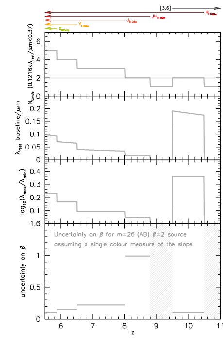
Figure 2: Top panel - The number of Hubble/WFC3 (Y_f098m, J_f125w, JH_f140w, and H_f160w) and Spitzer/IRAC ([3.6]) bands probing the rest frame $1216<\lambda_{\rm rest}/{\rm\AA}<3700$ UV continuum as a function of redshift. Second panel - The rest-frame UV wavelength baseline accessible by Hubble/WFC3 and Spitzer/IRAC observations as a function of redshift. Third panel - The ratio of the mean wavelength of the bluest and reddest filters to probe the rest-frame UV continuum. The arrows at the top denote the redshift range over which an individual band probes the rest-frame $1216<\lambda_{\rm rest}/{\rm\AA}<3700$ UV continuum. Bottom panel - The expected uncertainty on the measurement of $\beta$ as a function of redshift. This assumes a $\beta=-2$, $m=26$ source, for which $\beta$ is measured from the colour providing the longest usable wavelength baseline.

For $z>7$ galaxies, observations of the rest-frame UV continuum are typically limited to just 3 WFC3/IR bands uncontaminated by the Lyman-$\alpha$ break (i.e., $J_{f125w}$, $JH_{f140w}$, and $H_{f160w}$), and therefore suitable to measure the UV continuum slope $\beta$. This is demonstrated, in Figure 1, for sources at $z\in\{7,8,9,10\}$.

When only two bands are utilised for $UV$-continuum slope estimates, the relationship between the observed colour and UV continuum slope can simply be written as:

$$\beta=p\times(m_{1}-m_{2})_{\rm AB}-2,$$ (1)

where $(m_{1}-m_{2})_{\rm AB}$ is the observed colour assuming the AB magnitude system and $p$ is a value sensitive to the choice of bands. The value $p$ is approximately related to the ratio of the effective wavelengths ($\lambda_{1}$, $\lambda_{2}$) of the filters used to probe the slope, i.e.,

$$p^{-1}=2.5\cdot\log_{10}(\lambda_{1}/\lambda_{2}).$$ (2)

The value of $\log_{10}(\lambda_{1}/\lambda_{2})$ and the rest-frame UV wavelength baseline ($\lambda_{2}-\lambda_{1}$) accessible by Hubble/WFC3 and Spitzer/IRAC observations as a function of redshift are shown in Figure 2.

This accessible wavelength baseline is important as the uncertainty on $\beta$ will also scale with $p$. For example, at $z\sim 8$ where we only have observations using the JH_f140w and H_f160w bands, the value of $p$ using these bands is approximately $9.0$ (Bouwens et al. 2014a). A typical error on $m_{1}$ and $m_{2}$ of $0.1$ then translates into a large uncertainty on $\beta$ ($\approx 9.0\cdot\sqrt{0.1^{2}+0.1^{2}}\approx 1.3$). At $z>9.5$ the Spitzer/IRAC [3.6]-band probes the UV continuum, which, when combined with H_f160w-band observations, provides an especially extended wavelength baseline. The end result is a particularly small value for $p$ ($\approx 1.1$) and thus small uncertainty on $\beta$. This long wavelength baseline compensates for the lower sensitivity of observations with Spitzer/IRAC [3.6], allowing the the UV continuum to be estimated much more robustly than at $z\sim 8$ and on a par with $z\sim 6-8$ for the same observed apparent magnitude. This is demonstrated in the bottom panel of Figure 2.

The observed values of the UV-continuum slope $\beta$ for the $z\sim 10$ candidates (and the stack) are listed in Table 1 and shown in Figure 3. For the brightest candidate (GN-z10-1) we find $\beta_{\rm obs}=-2.1\pm 0.2$ while for the bright stack (see §2.1.1) we find $\beta_{\rm obs}=-2.1\pm 0.3$. If we stack only those sources which have $JH_{140}$-band observations (providing a second WFC3/IR filter where the $z\sim 10$ candidates are detected), i.e., GN-z10-1 and GN-z10-2, we find $\beta_{\rm obs}=-2.2\pm 0.3$.

While the formal random error on the mean $\beta$ is 0.2, at lower redshifts the $\beta$ distribution for luminous galaxies appears to show a significant intrinsic scatter of $\sigma_{\beta}\sim 0.35$ (Bouwens et al. 2009, 2012; Castellano et al. 2012; Rogers et al. 2014). Assuming a similar scatter at $z\sim 10$ translates to a slightly larger random error on the mean $\beta$ of 0.3.

2.2.1 Selection Biases

It is useful to consider briefly whether our mean $\beta$ results could be biased because of the selection criteria that were applied in searching for $z\sim 10$ galaxies. Such issues became an important aspect of the debate regarding $UV$-continuum slopes at $z\sim 7$ (e.g., Wilkins et al. 2012; Dunlop et al. 2012; Bouwens et al. 2012, 2014a), and it is important that we ensure that such issues do not become important again.

In identifying bright $z\sim 9$-10 candidates over CANDELS GOODS-S and GOODS-N, Oesch et al. (2014) did not consider sources with particularly red H${}_{f160w}-$[4.5]$>2$ colors redward of the Lyman break. Although the H${}_{f160w}-$[4.5] colour, unlike the H${}_{f160w}-$[3.6] colour, does not directly probe the UV continuum slope, they are correlated and noise in the two colors is not independent.. A colour of H${}_{f160w}-[4.5]\sim 2$ corresponds to $\beta\approx-0.1$. Given that all of our candidates have measured colors of $\beta<-1.8$ with small uncertainties, it is unlikely that a $\beta<-0.1$ selection will have an important impact on the mean $\beta$ measured for the sample, since the limit is $>3\sigma$ away from the mean $\beta$ observed and $3\sigma$ away from the mean $\beta$ assuming no evolution from $z\sim 5$-7.

It is encouraging that Bouwens et al. (2015a) selected exactly the same $z\sim 10$ candidates as Oesch et al. (2014), utilizing a slightly modified criteria (H${}_{f160w}-$[3.6]$<1.6$: corresponding to $\beta<-0.2$). This further confirms that the Oesch et al. (2014) sample of bright sources is not affected by strong $\beta$-dependent selection biases.

2.3 Possible Evolution in the observed UV-continuum slope

In the previous section, we presented the first determination of the mean $UV$-continuum slope $\beta$ for a multi-object sample at $z\sim 10$. Previously, UV continuum slopes for similarly luminous galaxies could only be determined up to $z\sim 8$ (Finkelstein et al. 2012).

With these new measurements in hand, it is interesting to look for evidence of evolution in the mean $\beta$ of galaxies versus redshift. Figure 4 presents the current measurements and compares it against previous measurements at $z\sim 4$-7 from Bouwens et al. (2014a) and Rogers et al. (2014).

As is evident from Figure 4, the observed UV continuum slopes of individual galaxies at $z\sim 10$ are found to be much bluer ($\Delta\beta\approx 0.4$) than those at $z\sim 4$-7. These new results are interesting, as they suggest either a gradual evolution in $\beta$ towards bluer colors or no evolution over a wide redshift baseline.

The comparison of measurements at $z=4$-7 with $z\sim 10$ is not necessarily straightforward as the $UV$-continuum slope is measured over very different wavelength baselines which may introduce a systematic bias. This is explored in more detail in Appendix A where we conclude that this is unlikely to be an important factor in this case, but could be as large as $\Delta\beta\sim 0.2$. If we allow for potential $\sim$10% systematics in our HST - IRAC color measurements (possible if the total magnitudes we estimate from the HST or Spitzer/IRAC data are not quite identical), the total systematic error relevant to the inferred evolution in $\beta$ could be as large as $\sim 0.22$.

Accounting for both random and systematic errors, we find the observed $\beta$ for luminous galaxies at $z\sim 10$ is only $1\sigma$ bluer than at $z\sim 7$. Therefore, our results are consistent with either a mild reddening of the $UV$-continuum slopes with cosmic time or no evolution at all.

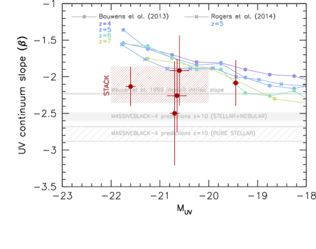
Figure 3: Mean value of the UV-continuum slope as a function of absolute rest-frame UV magnitude for candidate high-redshift ($z=4-10$) star forming galaxies (Bouwens et al. 2014; Rogers et al. 2014). The thin horizontal line denotes the intrinsic slope implicit in the empirical Meurer et al. (1999) relation and the two horizontal bands show the range of intrinsic slopes expected from the MassiveBlack-II hydrodynamical simulation at $z\sim 10$ assuming both $f_{\rm esc}=1$ (pure stellar) and $f_{\rm esc}=0$. It is important to note that at lower redshift the MassiveBlack-II simulation predicts significantly bluer intrinsic slopes (see Wilkins et al. 2013a).

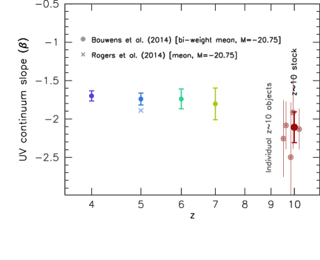
Figure 4: The observed UV continuum slope as a function of redshift for candidate high-redshift ($z=4-10$) star forming galaxies. Results at $z=4-7$ are based on the bi-weight mean of galaxies with $M_{1500}\approx-20.75$ from Bouwens et al. (2014a).

3 Inferred Dust Attenuation

3.1 Relating the observed UV continuum slope to dust attenuation

The presence of dust causes the observed UV continuum slope to redden relative to the intrinsic slope. The relationship between between the observed slope $\beta_{\,\rm obs}$ and the attenuation $A_{\lambda}$ can be written as (e.g. Meurer et al. 1999, Wilkins et al. 2013a),

$$A_{\lambda}=D_{\lambda}\times[\beta_{\,\rm obs}-\beta_{\,\rm int}],$$ (3)

where $\beta_{\rm int}$ is the intrinsic UV continuum slope, $\beta_{\rm obs}$ is the observed slope, and $D_{\lambda}$ ($={\rm d}A_{\lambda}/{\rm d}\beta$) describes the change in the attenuation as a function of the change in $\beta$, and is sensitive to the choice of attenuation/extinction curve. The intrinsic UV continuum slope is sensitive to a range of properties, including the star formation and metal enrichment histories, and the ionising photon escape fraction (see §3.2, and Wilkins et al. 2012, Wilkins et al. 2013a).

Both $\beta_{\rm int}$ and $D_{\lambda}$ can be constrained empirically (e.g. Meurer et al. 1999, Heinis et al. 2013) using a combination of rest-frame UV and far-IR observations of a sample of galaxies. $D_{\lambda}$ can be determined for any attenuation curve which extends over the rest-frame UV, and thus doesn’t necessarily require far-IR observations to be constrained.

3.2 The intrinsic UV continuum slope

Empirical constraints on $\beta_{\rm int}$ are, at present, due to the lack of sufficiently deep far-IR/sub-mm observations, limited to low-intermediate redshift (e.g. Heinis et al. 2013). The value of $\beta_{\rm int}$ at low/intermediate redshift is unlikely to reflect that at very-high redshift as $\beta_{\rm int}$ is sensitive to both the age and metallicity of the stellar population, both of which are expected to decrease in typical star forming galaxies to high-redshift (e.g. Wilkins et al. 2013a).

The sensitivity of the intrinsic UV-continuum slope $\beta_{\rm int}$ to various properties, including the joint distribution of stellar masses, ages, and metallicities (themselves determined the recent star formation and metal enrichment histories, and initial mass function) and the presence of nebular continuum, and to a lesser extent, line emission is discussed in Wilkins et al. (2012) and Wilkins et al. (2013a). We demonstrate this sensitivity in Figure 5 utilising the Pegase.2 stellar population synthesis code (Fioc & Rocca-Volmerange 1997, 1999). We determine the H${}_{f160w}-$[3.6] colour (our proxy for the UV continuum slope at $z\sim 10$) as a function of the duration of previous constant star formation, for two stellar metallicities, and also assuming $f_{\rm esc}=0$ and $f_{\rm esc}=1$ (i.e. a pure stellar continuum). Increasing the metallicity, the strength of nebular emission (i.e. decreasing the escape fraction $f_{\rm esc}$), and the duration of previous star formation all result in the intrinsic UV continuum slope becoming redder.

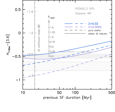
Figure 5: The sensitivity of the H_f160w-[3.6] colour (our proxy for the UV continuum slope) to the duration of previous (constant) star formation. The blue and purple lines show the result for $Z=0.02$ and $Z=0.0004$ respectively, while the solid and dashed lines show the result assuming $f_{\rm esc}=0$ (i.e. including nebular continuum and line emission) and $f_{\rm esc}=1$ (i.e. pure stellar emission) respectively. The solid and hatched horizontal bands show the predictions from the MassiveBlack-II simulations assuming $f_{\rm esc}=0$ and $f_{\rm esc}=1$ respectively.

3.2.1 Sensitivity to the candidate redshift

In addition to the physical properties outlined above the UV continuum slope inferred from observations will also be sensitive to the redshift of the source. This is demonstrated in Figure 6 where the predicted intrinsic H${}_{f160w}-$[3.6] colour (our proxy for the observed UV-continuum slope) of a stellar population that has been forming stars constantly for 50 Myr is shown as a function of redshift. Three different nebular emission scenarios are shown: (i) $f_{\rm esc}=1$ (i.e. pure stellar), (ii) $f_{\rm esc}=0$, and (iii) $f_{\rm esc}=1$ but with Lyman-$\alpha$ suppressed. In all three cases, in the interval $z=9.6-10.4$, the observed colour exhibits virtually no variation. At $z<9.6$ various strong emission lines, beginning with [OII]$\lambda 3727{\rm\AA}$, enter the Spitzer/IRAC [3.6]-band resulting in generally redder colours.

At $z>10.4$ the H_f160w-band filter overlaps with the wavelength of rest-frame Lyman-$\alpha$. Assuming no Lyman-$\alpha$ emerges (scenario iii) this results in the observed H_f160w-band encompassing the Lyman-$\alpha$ break resulting in a decreased flux, and consequently redder H${}_{f160w}-$[3.6] colours. If strong Lyman-$\alpha$ emerges the H${}_{f160w}-$[3.6] colour would rapidly become very blue before gradually becoming redder. Spectroscopic follow-up of $z\ga 6.5$ galaxies strongly points towards very little Ly$\alpha$ emission in $z\ga 10.4$ galaxies (e.g., Stark et al. 2010; Ono et al. 2012; Schenker et al. 2012; Pentericci et al. 2011; Caruana et al. 2012; Treu et al. 2013; Finkelstein et al. 2013; Oesch et al. 2015a: but see also Zitrin et al. 2015).

3.2.2 Simulation Predictions for the Intrinsic Slope

While empirical constraints on the intrinsic slope $\beta_{\rm int}$ exist they are only available at low-redshift, and are therefore unlikely to be representative of the very-high redshift Universe. We then also employ predictions from galaxy formation models for the intrinsic slope and spectral energy distribution. Specifically, we utilise predictions from the MassiveBlack and MassiveBlack-II hydro-dynamical simulations (see Khandai et al. 2015 for a general description of the simulations, and Wilkins et al. 2013a for predictions of the intrinsic UV continuum slope). At $z=10$ these simulations predict a median intrinsic slope of $\beta_{\rm int}\approx-2.54$ (assuming $f_{\rm esc}=0$) and $\beta_{\rm int}\approx-2.78$ for a pure stellar SED. In both cases the Pegase.2 SPS model is assumed, however other commonly used models models produce similar results (Wilkins et al. 2013ab).

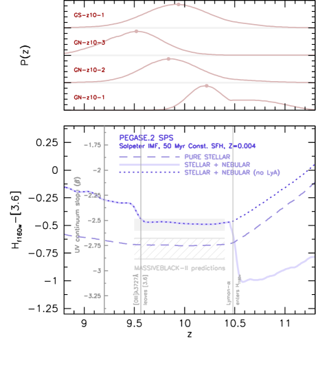
Figure 6: lower-panel The sensitivity of the H_f160w-[3.6] colour (our proxy for the UV continuum slope) to the redshift for a stellar population which has been constantly forming stars for 50 Myr (with $Z=0.004$, i.e. $\approx 1/5\,Z_{\odot}$). The three lines show the result of different nebular emission scenarios: (dashed) $f_{\rm esc}=1$ (i.e. pure stellar), (solid) $f_{\rm esc}=0$, and (dotted) $f_{\rm esc}=1$ but with Lyman-$\alpha$ suppressed. The predictions from MassiveBlack-II are shown by the shaded horizontal bands. upper-panel The redshift probability distributions of the 4 bright $z\sim 10$ candidates.

3.3 Inferred Dust Attenuation

By combining the observed UV continuum slope $\beta_{\rm obs}$ with a choice of intrinsic slope $\beta_{\rm int}$ and dust curve we can infer the level of dust attenuation using Equation 3. We do this both utilising the empirical Meurer relation and by assuming the intrinsic slope predicted by the MassiveBlack-II simulation combined with various attenuation/extinction curves.

In Figure 7 we first show the inferred UV attenuation assuming the empirical Meurer et al. (1999) relation. The combination of very blue observed colours and the $\beta\approx-2.23$ intrinsic slope implicit in the Meurer relation result in individual objects having best fit attenuations formally consistent with $A_{1500}=0$. The attenuation inferred from the bright stack is $A_{1500}=0.3\pm 0.5$.

Figure 8 is similar but instead shows the attenuation when we assume the intrinsic slope predicted by the MassiveBlack-II simulation (assuming $f_{\rm esc}=0.0$) along with both the Calzetti et al. (2000) and SMC (from Pei et al. 1992) dust curves. In this case all of the individual observations as well of the stack yield positive values of $A_{1500}$. If instead a higher escape fraction is assumed (which would make the intrinsic slope bluer) the inferred attenuation increases by between $0.25-0.5$ mags, depending on the choice of attenuation/extinction curve.

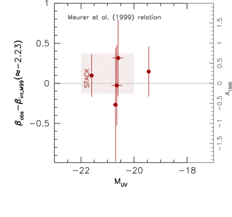
Figure 7: The inferred rest-frame UV attenuation $A_{1500}$ (right-hand axes) assuming the Meurer et al. (1999) relation.

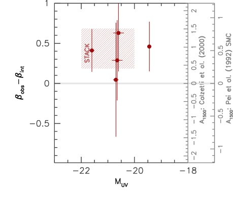
Figure 8: The inferred rest-frame UV attenuation $A_{1500}$ (right-hand axes) assuming the intrinsic slope predicted by MassiveBlack along with the Calzetti et al. (2000) starburst and Pei et al. (1992) SMC dust curves.

3.3.1 Evolution of dust attenuation

We now focus on the evolution of the rest-frame UV attenuation from $z\sim 10$ to $z=4-7$. In Figure 9 we compare our predictions for the UV attenuation at $z\sim 10$ to those at $z=4-7$ applying the same methodology - using both the Meurer et al. 1999 relation and by combining predictions of the intrinsic slope with the Calzetti et al. (2000) dust curve. Assuming a constant intrinsic slopes hints at a significant increase in the UV attenuation from $z\sim 10$ to $z\sim 7$ followed by little evolution between $z=7$ and $z=4$. Utilising the intrinsic slopes predicted by MassiveBlack (which vary with redshift) weakens this evolution.

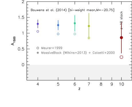
Figure 9: The evolution of the rest-frame UV attenuation $A_{1500}$ inferred from observations of the UV continuum slope in bright $z\in\{4,5,6,7,10\}$ star forming galaxies. Both the attenuation calculated using the Meurer et al. (1999) relation and combining the Calzetti et al. (2000) attenuation curve with the MassiveBlack predictions are shown.

4 Conclusions

Here we make use of the deep Hubble and Spitzer observations available over 5 particularly bright $z\sim 10$ candidates (Oesch et al. 2014; Zheng et al. 2012) to provide a first characterization of the mean UV-continuum slope for a multi-object sample of galaxies at $z\sim 10$.

We find:

• Combining Hubble and Spitzer we have measured the mean UV continuum slope of star formation galaxy candidates at $z\sim 10$. We find a mean $\beta$ of $-2.1\pm 0.3\pm 0.2$. We allow for up to a $0.2$ error in this measurement due to systematic errors that may derive from the wavelength baseline used to derive $\beta$ (Appendix A) or from small systematics in the photometry. The average observed UV continuum slope of a stack of bright $z\sim 10$ sources is only bluer than those at $z<8$ ($\beta_{\rm obs}\approx-1.7$) by $1\sigma$. These measurements are more robust than those at $z\sim 8$ due to the wide wavelength baseline provided by the combination of the Hubble/WFC3 H_f160w-band and Spitzer/IRAC [3.6]-band. The only previous measurement of $\beta$ at $z\sim 10$ was by Oesch et al. (2014) for the most luminous $z\sim 10$ galaxy in their selection.
  

• These slopes are redder than the intrinsic slope predicted by galaxy formation models, suggesting the existence of some dust attenuation, even at $z\approx 10$. For the brightest candidate, GN-z10-1 (Oesch et al. 2014), we infer a rest-frame UV attenuation of $\approx 0.9$ assuming the Calzetti et al. (2000) attenuation curve ($\approx 0.5$ assuming an SMC extinction law), while for the stack of bright candidates we find $0.9\pm 0.4$ assuming the Calzetti et al. (2000) law ($0.6\pm 0.2$ assuming an SMC extinction law).
  

4.1 Acknowledgements

We acknowledge useful conversations with Dan Coe on this topic, who has been attempting similar measurements on his triply imaged $z\sim 11$ candidate. SMW acknowledges support from the Science and Technology Facilities Council. IL acknowledges support from the European Research Council grant HIGHZ no. 227749 and the Netherlands Organisation for Scientific Research Spinoza grant. The Dark Cosmology Centre is funded by the Danish National Research Foundation.

Appendix A The effect of the wavelength baseline on the measured UV continuum slope

The UV continua of real stellar populations, though well approximated by, does not perfectly follow a power law. This effectively leaves the power law slope $\beta$ inferred from observations sensitive to the wavelength baseline of the observations.

In Figure 10 we demonstrate the difference between the UV continuum slope measured at $z=7$ using the $J_{f125w}-H_{f160w}$ colour and that measured at $z=10$ using the $H_{f160w}-$[3.6] colour for different durations of previous constant star formation and stellar metallicities. With the exception of very young durations of star formation the offset between the measured values of $\beta$ is fairly constant with star formation duration. However, the offset is strongly affected by the stellar metallicity. For example, for stellar metallicities of $Z=0.02$ there is a significant deviation between the two measures of $\beta$ with $\Delta\beta\approx 0.2$ suggesting that a much bluer value of $\beta$ would be measured at $z=10$ compared to $z=7$. However, for metallicities $Z=0.004-0.008$, which are expected to be typical of star forming galaxies at $Z=0.004-0.008$ (Wilkins et al., in-prep) this effect becomes small ($|\Delta\beta|<0.05$), though reverses at very-low metallicity.

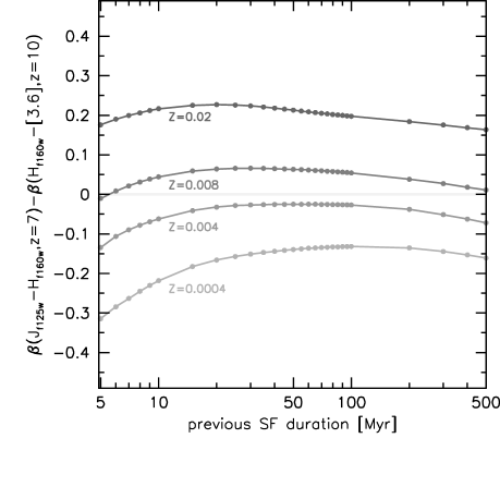
Figure 10: The difference between the UV continuum slope measured at $z=7$ using the $J_{f125w}-H_{f160w}$ colour and that measured at $z=10$ using the $H_{f160w}-$[3.6] colour as a function of the previous duration of (constant) star formation for 4 different metallicities ($Z\in\{0.0004,0.004,0.008,0.02\}$.

References

- [Ashby et al.(2013)] Ashby, M. L. N., Stanford, S. A., Brodwin, M., et al. 2013, ApJS, 209, 22
- [Ashby et al.(2015)] Ashby, M. L. N., Willner, S. P., Fazio, G. G., et al. 2015, ApJS, in press.
- [Bouwens et al.(2013)] Bouwens, R. J., Illingworth, G. D., Oesch, P. A., et al. 2014a, ApJ, 793, 115
- [Bouwens et al.(2012)] Bouwens, R. J., Bradley, L., Zitrin, A., et al. 2014b, ApJ, 795, 126
- [Bouwens et al.(2014)] Bouwens, R. J., Illingworth, G. D., Oesch, P. A., et al. 2015, ApJ, 803, 34
- [Bouwens et al.(2013)] Bouwens, R. J., Oesch, P. A., Illingworth, G. D., et al. 2013a, ApJ, 765, L16
- [Bouwens et al.(2015)] Bouwens, R. J., Oesch, P. A., Labbe, I., et al. 2015b, arXiv:1506.01035
- [Bouwens et al.(2012)] Bouwens, R. J., Illingworth, G. D., Oesch, P. A., et al. 2012, ApJ, 754, 83
- [Bouwens et al.(2011)] Bouwens, R. J., Illingworth, G. D., Oesch, P. A., et al. 2011b, ApJ, 737, 90
- [Bouwens et al.(2011)] Bouwens, R. J., Illingworth, G. D., Labbe, I., et al. 2011a, Nat, 469, 504
- [Bouwens et al.(2010)] Bouwens, R. J., Illingworth, G. D., Oesch, P. A., et al. 2010, ApJ, 709, L133
- [Bouwens et al.(2009)] Bouwens, R. J., Illingworth, G. D., Franx, M., et al. 2009, ApJ, 705, 936
- [Bouwens et al.(2008)] Bouwens, R. J., Illingworth, G. D., Franx, M., & Ford, H. 2008, ApJ, 686, 230
- [Bouwens et al.(2007)] Bouwens, R. J., Illingworth, G. D., Franx, M., & Ford, H. 2007, ApJ, 670, 928
- [Bouwens et al. 2006] Bouwens R. J. Illingworth G. D. Blakeslee J. P.; Franx M., 2006, ApJ, 653, 53
- [Bunker et al.(2010)] Bunker, A. J., Wilkins, S., Ellis, R. S., et al. 2010, MNRAS, 409, 855
- [Bradač et al.(2014)] Bradač, M., Ryan, R., Casertano, S., et al. 2014, ApJ, 785, 108
- [Brammer et al.(2013)] Brammer, G. B., van Dokkum, P. G., Illingworth, G. D., et al. 2013, ApJ, 765, L2
- [Calzetti et al.(2000)] Calzetti, D., Armus, L., Bohlin, R. C., et al. 2000, ApJ, 533, 682
- [Caruana et al.(2012)] Caruana, J., Bunker, A. J., Wilkins, S. M., et al. 2012, MNRAS, 427, 3055
- [Casey et al.(2014)] Casey, C. M., Narayanan, D., & Cooray, A. 2014, Phys. Rep., 541, 45
- [Coe et al.(2013)] Coe, D., Zitrin, A., Carrasco, M., et al. 2013, ApJ, 762, 32
- [da Cunha et al.(2013)] da Cunha, E., Groves, B., Walter, F., et al. 2013, ApJ, 766, 13
- [Dressel et al. (2012)] Dressel, L., et al. 2012. “Wide Field Camera 3 Instrument Handbook, Version 5.0” (Baltimore: STScI)
- [Dunlop et al.(2013)] Dunlop, J. S., Rogers, A. B., McLure, R. J., et al. 2013, MNRAS, 432, 3520
- [Dunlop et al.(2012)] Dunlop, J. S., McLure, R. J., Robertson, B. E., et al. 2012, MNRAS, 420, 901
- [Ellis et al.(2013)] Ellis, R. S., McLure, R. J., Dunlop, J. S., et al. 2013, ApJ, 763, L7
- [Finkelstein et al.(2012)] Finkelstein, S. L., Papovich, C., Salmon, B., et al. 2012, ApJ, 756, 164
- [Finkelstein et al.(2010)] Finkelstein, S. L., Papovich, C., Giavalisco, M., et al. 2010, ApJ, 719, 1250
- [Finkelstein et al.(2013)] Finkelstein, S. L., Papovich, C., Dickinson, M., et al. 2013, Nat, 502, 524
- [Fioc & Rocca-Volmerange(1999)] Fioc, M., & Rocca-Volmerange, B. 1999, arXiv:astro-ph/9912179
- [Fioc & Rocca-Volmerange(1997)] Fioc, M., and Rocca-Volmerange, B. 1997, A&A, 326, 950
- [González et al.(2014)] González, V., Bouwens, R., Illingworth, G., et al. 2014, ApJ, 781, 34
- [González et al.(2010)] González, V., Labbé, I., Bouwens, R. J., et al. 2010, ApJ, 713, 115
- [Grogin et al.(2011)] Grogin, N. A., Kocevski, D. D., Faber, S. M., et al. 2011, ApJS, 197, 35
- [Hathi et al.(2013)] Hathi, N. P., Cohen, S. H., Ryan, R. E., Jr., et al. 2013, ApJ, 765, 88
- [Heinis et al.(2013)] Heinis, S., Buat, V., Béthermin, M., et al. 2013, MNRAS, 429, 1113
- [Illingworth et al.(2013)] Illingworth, G. D., Magee, D., Oesch, P. A., et al. 2013, ApJS, 209, 6
- [Ishigaki et al.(2015)] Ishigaki, M., Kawamata, R., Ouchi, M., et al. 2015, ApJ, 799, 12
- [Khandai et al.(2015)] Khandai, N., Di Matteo, T., Croft, R., et al. 2015, MNRAS, 450, 1349
- [Koekemoer et al.(2013)] Koekemoer, A. M., Ellis, R. S., McLure, R. J., et al. 2013, ApJS, 209, 3
- [Koekemoer et al.(2011)] Koekemoer, A. M., Faber, S. M., Ferguson, H. C., et al. 2011, ApJS, 197, 36
- [Kron (1980)] Kron, R. G. 1980, ApJS, 43, 305
- [Kurczynski et al.(2014)] Kurczynski, P., Gawiser, E., Rafelski, M., et al. 2014, ApJ, 793, L5
- [Labbé et al.(2006)] Labbé, I., Bouwens, R., Illingworth, G. D., & Franx, M. 2006, ApJ, 649, L67
- [Labbé et al.(2010)] Labbé, I., et al. 2010, ApJ, 708, L26
- [Labbé et al.(2013)] Labbé, I., Oesch, P. A., Bouwens, R. J., et al. 2013, ApJ, 777, L19
- [Labbe et al.(2015)] Labbe, I., Oesch, P. A., Illingworth, G. D., et al. 2015, ApJS, in press, arXiv:1507.08313
- [Lehnert & Bremer(2003)] Lehnert, M. D., & Bremer, M. 2003, ApJ, 593, 630
- [McLure et al.(2013)] McLure, R. J., Dunlop, J. S., Bowler, R. A. A., et al. 2013, MNRAS, 432, 2696
- [McLure et al.(2011)] McLure, R. J., Dunlop, J. S., de Ravel, L., et al. 2011, MNRAS, 418, 2074
- [Meurer et al.(1999)] Meurer, G. R., Heckman, T. M., & Calzetti, D. 1999, ApJ, 521, 64
- [Oesch et al.(2010)] Oesch, P. A., Bouwens, R. J., Illingworth, G. D., et al. 2010, ApJ, 709, L16
- [Oesch et al.(2012)] Oesch, P. A., Bouwens, R. J., Illingworth, G. D., et al. 2012, ApJ, 759, 135
- [Oesch et al.(2013)] Oesch, P. A., Bouwens, R. J., Illingworth, G. D., et al. 2013, ApJ, 773, 75
- [Oesch et al.(2014)] Oesch, P. A., Bouwens, R. J., Illingworth, G. D., et al. 2014, ApJ, 786, 108
- [Oesch et al.(2015)] Oesch, P. A., van Dokkum, P. G., Illingworth, G. D., et al. 2015a, ApJ, 804, L30
- [Oesch et al.(2015)] Oesch, P. A., Bouwens, R. J., Illingworth, G. D., et al. 2015b, ApJ, 808, 104
- [Oke & Gunn 1983] Oke J. B., Gunn J. E., 1983, ApJ, 266, 713
- [Ono et al.(2012)] Ono, Y., Ouchi, M., Mobasher, B., et al. 2012, ApJ, 744, 83
- [Papovich et al.(2004)] Papovich, C., Dickinson, M., Ferguson, H. C., et al. 2004, ApJ, 600, L111
- [Pei(1992)] Pei, Y. C. 1992, ApJ, 395, 130
- [Pentericci et al.(2011)] Pentericci, L., Fontana, A., Vanzella, E., et al. 2011, ApJ, 743, 132
- [Postman et al.(2012)] Postman, M., Coe, D., Benítez, N., et al. 2012, ApJS, 199, 25
- [Reddy et al.(2010)] Reddy, N. A., Erb, D. K., Pettini, M., Steidel, C. C., & Shapley, A. E. 2010, ApJ, 712, 1070
- [Robertson et al.(2013)] Robertson, B. E., Furlanetto, S. R., Schneider, E., et al. 2013, ApJ, 768, 71
- [Rogers et al.(2014)] Rogers, A. B., McLure, R. J., Dunlop, J. S., et al. 2014, MNRAS, 440, 3714
- [Salmon et al.(2014)] Salmon, B., Papovich, C., Finkelstein, S. L., et al. 2015, ApJ, 799, 183
- [Salpeter 1955] Salpeter E. E., 1955, ApJ, 121, 161
- [Schaerer et al.(2013)] Schaerer, D., de Barros, S., & Sklias, P. 2013, A&A, 549, A4
- [Schaerer & de Barros(2010)] Schaerer, D., & de Barros, S. 2010, A&A, 515, A73
- [Schenker et al.(2012)] Schenker, M. A., Stark, D. P., Ellis, R. S., et al. 2012, ApJ, 744, 179
- [Schmidt et al.(2014)] Schmidt, K. B., Treu, T., Trenti, M., et al. 2014, ApJ, 786, 57
- [Shim et al.(2011)] Shim, H., Chary, R.-R., Dickinson, M., et al. 2011, ApJ, 738, 69
- [Smit et al.(2014)] Smit, R., Bouwens, R. J., Labbé, I., et al. 2014, ApJ, 784, 58
- [Spitler et al.(2014)] Spitler, L. R., Straatman, C. M. S., Labbé, I., et al. 2014, ApJ, 787, L36
- [Stanway, McMahon & Bunker 2005] Stanway E. R., McMahon R. G., Bunker A. J., 2005, MNRAS, 359, 1184
- [Stark et al.(2010)] Stark, D. P., Ellis, R. S., Chiu, K., Ouchi, M., & Bunker, A. 2010, MNRAS, 408, 1628
- [Stark et al.(2013)] Stark, D. P., Schenker, M. A., Ellis, R., et al. 2013, ApJ, 763, 129
- [Stark et al.(2009)] Stark, D. P., Ellis, R. S., Bunker, A., et al. 2009, ApJ, 697, 1493
- [Symeonidis et al.(2013)] Symeonidis, M., Vaccari, M., Berta, S., et al. 2013, MNRAS, 431, 2317
- [Treu et al.(2013)] Treu, T., Schmidt, K. B., Trenti, M., Bradley, L. D., & Stiavelli, M. 2013, ApJ, 775, LL29
- [Wilkins et al.(2013)] Wilkins, S. M., Coulton, W., Caruana, J., et al. 2013b, MNRAS, 435, 2885
- [Wilkins et al.(2013)] Wilkins, S. M., Bunker, A., Coulton, W., et al. 2013a, MNRAS, 430, 2885
- [Wilkins et al.(2012)] Wilkins, S. M., Gonzalez-Perez, V., Lacey, C. G., & Baugh, C. M. 2012, MNRAS, 424, 1522
- [Wilkins et al.(2011)] Wilkins, S. M., Bunker, A. J., Stanway, E., Lorenzoni, S., & Caruana, J. 2011b, MNRAS, 417, 717
- [Wilkins et al.(2011)] Wilkins, S. M., Bunker, A. J., Lorenzoni, S., & Caruana, J. 2011a, MNRAS, 411, 23
- [Wilkins et al.(2010)] Wilkins, S. M., Bunker, A. J., Ellis, R. S., et al. 2010, MNRAS, 403, 938
- [Zheng et al.(2012)] Zheng, W., Postman, M., Zitrin, A., et al. 2012, Nat, 489, 406
- [Zitrin et al.(2014)] Zitrin, A., Zheng, W., Broadhurst, T., et al. 2014, ApJ, 793, L12
- [Zitrin et al.(2015)] Zitrin, A., Labbe, I., Belli, S., et al. 2015, ApJ, submitted, arXiv:1507.02679