Adaptive model reduction for nonsmooth discrete element simulation

Abstract

A method for adaptive model order reduction for nonsmooth discrete element simulation is developed and analysed in numerical experiments. Regions of the granular media that collectively move as rigid bodies are substituted with rigid bodies of the corresponding shape and mass distribution. The method also support particles merging with articulated multibody systems. A model approximation error is defined and used to derive conditions for when and where to apply reduction and refinement back into particles and smaller rigid bodies. Three methods for refinement are proposed and tested: prediction from contact events, trial solutions computed in the background and using split sensors. The computational performance can be increased by 5 - 50 times for model reduction level between 70 - 95 %.

1 Introduction

Simulation of granular matter is important for increased understanding of the nature of granular media and as an engineering tool for design, control and optimization of processing and transportation systems [1]. With the discrete element method (DEM) the material is modeled as a system of contacting rigid bodies, referred to as particles in this text. This provides detailed information about force structures and particle kinematics on a microscopic level. DEM accurately capture many of the characteristic phenomena of granular media - for instance jamming, dilatancy, emergence of strong force chains, strain localization, avalanches and size-segregation upon fluidization - that are difficult or even impossible to model with continuum based methods. The required computational time increase with the number of bodies and this limit the practical use of DEM for exhaustive simulation studies of large-scale systems and large parameter spaces. One strategy to remedy this is to increase the computational performance by use of parallel algorithms and dedicated hardware. Another strategy is the use of implicit integration with large time-step using the nonsmooth DEM (NDEM) [2], also known as the contact dynamics method [3, 4], where velocities may be time-discontinuous and impulses can propagate instantly through the system.

A third strategy, that is pursued in the paper, is to reduce the computational complexity by identifying regions in the granular media where the particles may be substituted by approximate models with less degrees of freedom.

1.1 Previous work

Model order reduction is well established and widely used for reducing the computational complexity in solid and fluid mechanics, dynamical systems and control theory [6, 5]. In multibody dynamics, it is often used for reducing the degrees of freedom of flexible bodies [7] while the number of multibodies are preserved. There are few examples that resemble model order reduction for the discrete element method. Glössmann [8] applied the Karhunen-Loéve transform to clusters of discrete elements that show dynamic coherence to reduce the order of generalized coordinates. In the combined finite-discrete element method (FDEM) each body is represented as a discrete element that is also discretized by a finite element method [9]. The bodies may deform, fracture and fragment indefinitely into smaller elements based on the internal stresses. An inversion of this is the hierarchical multiscale modeling of granular media discretized by a coarse mesh of finite elements in combination with assemblies of fine grained discrete elements for numerical computation of the local constitutive law for the finite element computations [10, 11]. A two-scale and two-method approach for modeling granular materials is presented in [12], where DEM is used for domains of large and discontinuous deformations and as an elastoplastic solid using FEM in continuous domains. Automatic simplification algorithms of articulated multibody systems have been developed and shown to increase computational performance by two orders in magnitude on large-scale linkage systems [13, 14]. Dynamic formation of both rigid aggregates (clumped particles) and elastic aggregates (clustered particles), are supported by several discrete element codes and is used for modeling grains in brittle rock [15].

1.2 Outline of the idea and the challenges

The idea is to identify regions of the granular media that collectively move as rigid bodies and substitute each of these regions with rigid aggregates of the corresponding shape and mass distribution. Particles and rigid aggregates may also merge with rigid bodies or kinematic geometries that do not represent granular media, for instance the particles in an excavator bucket may merge with the bucket into one single rigid body. The aggregated rigid bodies still contribute to the system dynamics but require only a few degrees of freedom. When merged material is disturbed, by a change in external forces or boundary contacts, it may split into smaller constituents that are either rigid aggregates of fewer particles or single particles.

The complexity of systems with granular media in the solid state is thus largely reduced and the computational performance increase correspondingly while the macroscopic dynamics may be preserved. For granular media in the gaseous or liquid state, on the other hand, a model reduction into rigid aggregates will cause significant errors. This paper is limited to model reduction into rigid bodies. The extension to elastoplastic bodies can be imagined but is beyond the current scope. The ultimate goal is to achieve optimal trade-off between: maximum system reduction; minimum errors on the macroscopic dynamics; minimum computational overhead.

The main challenge is to predict when and where merged material should be refined, or split. Most real systems are in a combination of the three states of granular media: solid, fluid and gas [16]. If the split conditions are too restrictive, or the merge condition too progressive, the bulk properties become wrong. This may appear as incorrect angle of repose, artificial resistance to compression and shearing forces and erroneous rheology in the fluid state. If the split conditions are too permissive, or the merge conditions too strict, most particle will remain free and the there is no computational gain. Also, the computational overhead of model reduction must be small in comparison to the computational time for the fully resolved system.

The idea is illustrated in Fig. 1 with an excavator digging in a bed of granular material. Only a finite domain of the material around the bucket is displaced and need to be simulated dynamically. The remaining part is static and contribute merely with supporting contact pressure. When the bucket is filled and starts to lift, most material co-move rigidly with the bucket. If the purpose of the simulation is to compute the dynamics of the excavator and the load forces in the mechanism, the material and the bucket can be approximated by a single rigid body. When the bucket accelerates or rotate slowly the force distribution in the granular material change and it might start to flow. Several methods for predicting splitting of the rigid aggregates are proposed and tested in numerical experiments. The method are based either on contact events or estimating force distribution or particle motion by computations in the background.

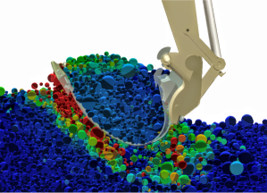
Figure 1: Illustration of model reduction in an excavation scenario simulated without model reduction. The particles are color coded by velocity from blue (stationary) to red. Most particles in the bed are in relative rest and would be well described by a single rigid body. The particles in the excavator bucket may be aggregated with the bucket into a single rigid body. The main challenge is to predict when and where the merged material should split.

2 Particles, rigid aggregate and multibodies

This section is devoted to the mathematical representation of contacting particles and rigid bodies as multibody systems with nonsmooth dynamics and kinematic constraints.

2.1 Global system variables

The variables for particles, rigid aggregates and other rigid bodies are components of the global system variables that we denote $\textbf{x},\textbf{v},\bm{f}$ and M and refer to as generalized position, velocity, force and mass although they are concatenations of linear and rotational degrees of freedom. Quaternions are used for representing orientations. The matrix dimension of the global quantities are $\dim(\textbf{x})=7N_{\text{b}}$, $\dim(\textbf{v})=\dim(\textbf{f})=6N_{\text{b}}$, $\dim(\textbf{M})=6N_{\text{b}}\times 6N_{\text{b}}$, where ${N}_{\text{b}}$ is the total number of bodies.

2.2 Nonsmooth multibody dynamics

The following equations of motion for nonsmooth multibody dynamics are assumed:

$$\textbf{M}\dot{\textbf{v}}+\dot{\textbf{M}}\textbf{v} = {\textbf{f}}_{\text{ext}}+{\textbf{G}}_{\text{n}}^{\text{T}}{\bm{\lambda}}_{\text{n}}+{\textbf{G}}_{\text{t}}^{\text{T}}{\bm{\lambda}}_{\text{t}}+{\textbf{G}}_{\text{r}}^{\text{T}}{\bm{\lambda}}_{\text{r}}+{\textbf{G}}_{\text{j}}^{\text{T}}{\bm{\lambda}}_{\text{j}},$$ (1)

$$0\leq{\varepsilon}_{\text{n}}{\bm{\lambda}}_{\text{n}}+{\textbf{g}}_{\text{n}}+{\tau}_{\text{n}}{\textbf{G}}_{\text{n}}\textbf{v} \perp {\bm{\lambda}}_{\text{n}}\geq 0,$$ (2)

$${\gamma}_{\text{t}}{\bm{\lambda}}_{\text{t}}+{\textbf{G}}_{\text{t}}\textbf{v} = 0,\ \ |{\bm{\lambda}}_{\text{t}}^{(\alpha)}|\leq{\mu}_{\text{t}}|\textbf{G}_{\text{n}}^{(\alpha){\text{T}}}{\lambda}_{\text{n}}^{(\alpha)}|,$$ (3)

$${\gamma}_{\text{r}}{\bm{\lambda}}_{\text{r}}+{\textbf{G}}_{\text{r}}\textbf{v} = 0,\ \ |{\bm{\lambda}}_{\text{r}}^{(\alpha)}|\leq{\mu}_{\text{r}}r|\textbf{G}_{\text{n}}^{(\alpha){\text{T}}}{\lambda}_{\text{n}}^{(\alpha)}|,$$ (4)

$${\varepsilon}_{\text{j}}{\bm{\lambda}}_{\text{j}}+{\eta}_{\text{j}}{\textbf{g}}_{\text{j}}+{\tau}_{\text{j}}{\textbf{G}}_{\text{j}}\textbf{v} = 0.$$ (5)

The first equation is the Newton-Euler equation of motion for rigid bodies with external (smooth) forces ${\textbf{f}}_{\text{ext}}$ and constraint force ${\textbf{G}}_{\text{}}^{\text{T}}\bm{\lambda}$ with Lagrange multiplier $\bm{\lambda}$ and Jacobian G, divided into normal (n), tangential (t), rolling (r) and articulated and possibly motorized joints (j). Details are found in the Appendix. Equations (2)-(3) are the Signorini-Coulomb conditions with constraint regularization and stabilization terms ${\varepsilon}_{\text{n}}$, ${\tau}_{\text{n}}$ and ${\gamma}_{\text{t}}$. With ${\varepsilon}_{\text{n}}={\tau}_{\text{n}}=0$, Eq. (2) state that bodies should be separated or have zero overlap, ${\textbf{g}}_{\text{n}}(\textbf{x})\geq 0$, and if so the normal force should be non-cohesive, ${\bm{\lambda}}_{\text{n}}\geq 0$. With ${\gamma}_{\text{t}}=0$, Eq. (3) state that contacts should have zero relative slide velocity, ${\textbf{G}}_{\text{t}}\textbf{v}=0$, provided that the friction force remain bounded by the Coulomb friction law with friction coefficient ${\mu}_{\text{t}}$. Eq. (4) similarly constrains relative rotation of contacting bodies provided the constraint torque do not exceed the rolling resistance law with rolling resistance coefficient ${\mu}_{\text{r}}$ and radius $r$. The constraint force, ${\textbf{G}}_{\text{j}}^{\text{T}}{\bm{\lambda}}_{\text{j}}$, arise for articulated rigid bodies jointed with kinematic links and motors represented with the generic constraint equation (5). With ${\varepsilon}_{\text{j}},{\tau}_{\text{j}}=0$ and ${\eta}_{\text{j}}=1$, it become an ideal holonomic constraint $\textbf{g}(\textbf{x})=0$. For $\varepsilon,\eta=0$ and $\tau=1$, it become an ideal Pfaffian constraint $\textbf{G}\dot{\textbf{x}}=0$. With $\varepsilon,\eta,\tau\neq 0$ it can represent a generic constraint with compliance and damping. The set of equations (1)-(5) may thus model granular materials strongly coupled with mechatronic systems, e.g., vehicles, robots and mechanical processing units.

The Lagrange multiplier become an auxiliary variable to solve for in addition to position and velocity. The regularization and stabilization terms, $\varepsilon$ and $\gamma$, introduce compliance and dissipation in motion orthogonal to the constraint manifold. In the absence of the inequality and complementarity conditions, the regularized constraints may be viewed as Legendre transforms of a potential and Rayleigh dissipation function of the form $U_{\varepsilon}(\textbf{x})=\tfrac{1}{2\varepsilon}\textbf{g}^{T}\textbf{g}$ and $\mathcal{R}_{\gamma}(\textbf{x},\textbf{v})=\tfrac{1}{2\gamma}(\textbf{G}\textbf{v})^{T}(\textbf{G}\textbf{v})$ [17, 18]. This enable modeling of arbitrarily stiff elastic and viscous interactions in terms of constraint forces with direct mapping between the regularization and stabilization terms to physical material parameters. This is applied to map the stiffness and damping terms from the nonlinear Hertz contact law, or linear spring and dashpot, from conventional (smooth) discrete element method to the constraint based and nonsmooth discrete element method. The detailed constraints, Jacobians and parameters are found in Ref. [19] and summarized in Appendix A together with the numerical integration scheme used in this paper.

The dynamics is allowed to be nonsmooth which means that velocities may change discontinuously in time. Impacts and frictional stick-slip transitions may thus be considered as instantaneous events and propagate immediately through the entire system by an impulse transfer altering the velocities from $\textbf{v}_{-}$ to $\textbf{v}_{+}$. The contacts are divided into impacts and continuous contacts, depending on the magnitude of the incoming relative normal velocities ${\textbf{G}}_{\text{n}}\textbf{v}_{-}$. The impulse transfer through the system should satisfy the Newton impact law, ${\textbf{G}}_{\text{n}}^{(n)}\textbf{v}_{+}=-e{\textbf{G}}_{\text{n}}^{(n)}\textbf{v}_{-}$, with coefficient of restitution $e$ for the impacts $(n)$, as well as preserve all remaining constraints $(m)$ on velocity level, $\textbf{G}^{(m)}\textbf{v}_{+}=0$.

2.3 Particles

Each elementary granule is referred to as a particle and is modeled as a rigid body with solid geometry. A particle is either free or part of a rigid aggregate of particles. Each free particle is represented by a dynamic discrete element obeying the equation of motions in Sec. 2.2 and may interact with other particles and rigid aggregate bodies via contacts. Each particle that is part of a rigid aggregate is a kinematic discrete element that co-move rigidly with the aggregate body. No forces are applied to aggregated particles. For simplicity, particles are assumed spherical but can easily be extended to more general geometric shapes. Reference to a specific particle is made by latin indices, e.g., $a,b,\ldots=1,2,\ldots,N_{\text{p}}$, and we use square brackets to emphasize particle index. We use the notations $\vec{\bm{x}}_{[a]},\vec{\bm{v}}_{[a]},\vec{\bm{f}}_{[a]}$, $m_{[a]}$ and $d_{[a]}$ for position, translational velocity, force, mass and diameter, and $\vec{\bm{e}}_{[a]},\vec{\bm{\omega}}_{[a]},\vec{\bm{\tau}}_{[a]}$ and $\bm{I}_{[a]}$, for orientation, angular velocity, torque and inertia tensor. Spatial components of a vector or matrix is indexed by $\alpha,\beta=1,2,3$ referring to the $x,y,z$ axes in a global Cartesian coordinate system, e.g., $x^{[a]}_{\alpha}$ and $I_{\alpha\beta}$. We concatenate these variables into a particle’s generalized position, velocity, force and mass, denoted $\textbf{x}_{[a]},\textbf{v}_{[a]},\textbf{f}_{[a]}$ and $\textbf{M}_{[a]}$, with $\textbf{v}_{[a]}=(\vec{\bm{v}}_{[a]}^{\text{T}},\vec{\bm{\omega}}_{[a]}^{\text{T}})^{\text{T}}$ etc. and $\textbf{M}_{[a]}=\text{diag}(m_{[a]}\bm{1}_{3\times 3},\bm{I}_{[a]})$.

2.4 Rigid aggregates

A rigid aggregate, or just aggregate, is a rigid body that represent an aggregate of particles co-moving as a single rigid body. The rigidity is an assumed collective result of the contact forces creating a jammed state although no such internal forces are modeled or computed explicitly. The variables of rigid aggregates are represented with similar notations as for particles, e.g., $\textbf{x}_{[A]}$ and $\textbf{M}_{[A]}$, but with capital latin indices $A,B,\ldots=1,2,\ldots,{N}_{\text{a}}$. The set of particles that constitute an aggregate $A$ is denoted $\mathcal{N}_{A}$. The relation between the dynamic variables of the aggregate and the particles are illustrated in Fig. 2 and computed as follows:

$$m_{[A]} = \sum_{a\in\mathcal{N}_{A}}m_{[a]},$$ (6)

$$\vec{\bm{x}}_{[A]} = m_{[A]}^{-1}\sum_{a\in\mathcal{N}_{A}}m_{[a]}\vec{\bm{x}}_{[a]},$$ (7)

$$\vec{\bm{v}}_{[A]} = m_{[A]}^{-1}\sum_{a\in\mathcal{N}_{A}}m_{[a]}\vec{\bm{v}}_{[a]},$$ (8)

$$I^{[A]}_{\alpha\beta} = \sum_{a\in\mathcal{N}_{A}}m_{[a]}\left(|\vec{\bm{r}}_{[aA]}|^{2}\delta_{\alpha\beta}-r^{[aA]}_{\alpha}r^{[aA]}_{\beta}\right),$$ (9)

$$\vec{\bm{\omega}}_{[A]} = \bm{I}^{-1}_{[A]}\sum_{a\in\mathcal{N}_{A}}m_{[a]}\vec{\bm{r}}_{[aA]}\times\vec{\bm{v}}_{[aA]},$$ (10)

where $\vec{\bm{r}}_{[aA]}=\vec{\bm{x}}_{[a]}-\vec{\bm{x}}_{[A]}$ and $\vec{\bm{v}}_{[aA]}=\vec{\bm{v}}_{[a]}-\vec{\bm{v}}_{[A]}$. The kinematics of the aggregated particles $a\in\mathcal{N}_{A}$ is

$$\vec{\bm{x}}_{[a]} = \vec{\bm{x}}_{[A]}+\vec{\bm{r}}_{[aA]},$$ (11)

$$\vec{\bm{v}}_{[a]} = \vec{\bm{v}}_{[A]}+\vec{\bm{\omega}}_{[A]}\times\vec{\bm{r}}_{[aA]},$$ (12)

$$\vec{\bm{\omega}}_{[a]} = \vec{\bm{\omega}}_{[A]}.$$ (13)

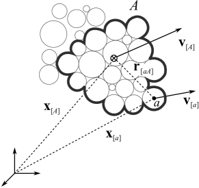
Figure 2: Illustration of a rigid aggregate of contacting particles and some free particles.

2.5 Multibodies

By elementary rigid bodies it is meant bodies that represent other than granular bodies, e.g., part of an articulated multibody. Elementary rigid bodies are also included in model reduction and may form reduced aggregates with both elementary rigid bodies and particles. But the additional complexity of merge and split conditions in articulated system is not covered here. For convenience elementary rigid bodies are represented with the same notation as used for aggregates, that is, capital index in square brackets $[A]$.

2.6 Contacts

The set of contacts is denoted ${\mathcal{N}}_{\text{c}}$. Integer $n=1,2,\ldots,{N}_{\text{c}}$ is used for contact index and this is emphasized by round brackets, e.g., $g^{(n)}$. The gap function $\delta(\textbf{x})$ measure the magnitude of overlap between two contacting bodies. Contact forces and velocities are sometimes decomposed in the directions of contact normal, $\vec{\textbf{n}}$ and tangents, $\vec{\mathbf{t}}_{1}$ and $\vec{\mathbf{t}}_{2}$. The relative velocity at a contact $n$ between a particle $a$ and a rigid body $A$ can thus be written $\vec{\bm{u}}^{(n)}=\vec{\bm{v}_{[a]}}+\vec{\bm{\omega}}_{[a]}\times\vec{\bm{d}}^{(n)}_{[a]}-\vec{\bm{v}}_{[A]}-\vec{\bm{\omega}}_{[A]}\times\vec{\bm{d}}^{(n)}_{[A]}$, where $\vec{\bm{d}}^{(n)}_{[a]}$ is the position of the contact point relative to $\vec{\bm{x}}_{[a]}$ and $\vec{\bm{d}}^{(n)}_{[A]}$ relative to $\vec{\bm{x}}_{[A]}$.

3 Adaptive model order reduction

Let the following equations represent the full system of particles and elementary rigid bodies coupled with constraints

$$\textbf{M}\ddot{\textbf{x}}+\dot{\textbf{M}}\dot{\textbf{x}} = {\textbf{f}}_{\text{ext}}+\textbf{G}^{\text{T}}\bm{\lambda},$$ (14)

$$\varepsilon\bm{\lambda}+\eta\textbf{g}(\textbf{x})+\tau\textbf{G}\dot{\textbf{x}} = 0,$$ (15)

having solution $\textbf{x}\in\mathbb{R}^{n}$ and $\bm{\lambda}\in\mathbb{R}^{m}$. The constraint equation (15) represent the collection of both position and velocity constraints and it is assumed to be appended with additional inequalities and complementarity conditions for the multiplier. The full system, (14)-(15), is approximated with a reduced system $\tilde{\textbf{x}}\in\mathbb{R}^{\tilde{n}}$ and $\tilde{\bm{\lambda}}\in\mathbb{R}^{\tilde{m}}$ with less degrees of freedom $\tilde{n}<n$ and $\tilde{m}<m$. The reduced system belong to a subspace of the full system. We define the model order reduction level as $h=1-\tilde{n}/n$. When $h\to 1$ the system is maximally reduced to one single rigid body and when $h=0$ it is fully resolved in all free particles. The approximate relation between the reduced and full system is expressed using subspace transformation matrices $\textbf{P}\in\mathbb{R}^{n\times\tilde{n}}$ and $\textbf{Q}\in\mathbb{R}^{m\times\tilde{m}}$ such that

x $$\approx \textbf{P}\tilde{\textbf{x}},$$ (16)

$$\bm{\lambda} \approx \textbf{Q}\tilde{\bm{\lambda}}.$$ (17)

Given a rigid aggregate, the transformation matrix P is easily constructed from the rigid transformations in Eq. (11), that relate the positions of the aggregated particles relative to the aggregate centre. In a rigid aggregate the inter-particle constraints are redundant. The transformation matrix Q eliminate the redundant equations when a rigid aggregate is substituted for a collection of particles. The reduced multibody system become

$$\tilde{\textbf{M}}\ddot{\tilde{\textbf{x}}} = {\tilde{\textbf{f}}}_{\text{e}}+\tilde{\textbf{G}}^{\text{T}}\tilde{\bm{\lambda}},$$ (18)

$$\varepsilon\tilde{\bm{\lambda}}+\eta\tilde{\textbf{g}}(\tilde{\textbf{x}})+\tau\tilde{\textbf{G}}\dot{\tilde{\textbf{x}}} = 0$$ (19)

with $\tilde{\textbf{M}}=\textbf{P}\textbf{M}\textbf{P}^{T}$, ${\tilde{\textbf{f}}}_{\text{e}}=\textbf{P}{\textbf{f}}_{\text{ext}}-\dot{\tilde{\textbf{M}}}\dot{\tilde{\textbf{x}}}$, $\tilde{\textbf{G}}=\textbf{Q}^{T}\textbf{G}\textbf{P}$, $\tilde{\bf{\lambda}}=\textbf{Q}\bm{\lambda}$, $\tilde{\textbf{g}}=\textbf{Q}\textbf{g}$. Note that $\dot{\tilde{\textbf{M}}}\dot{\tilde{\textbf{x}}}$ is included as an explicit force in ${\tilde{\textbf{f}}}_{\text{e}}$ as is common and often referred to as the gyroscopic force. If the complexity of the reduced system is much smaller than the original, $\tilde{n}\ll n$ and $\tilde{m}\ll m$, the computational efficiency can increase dramatically.

The reduced system can, however, expected to deviate more or less from the original system. The model reduction may be applied adaptively to keep the approximation error below a specified error tolerance. The approximation error is defined

$$\mathcal{E}(t)=\textbf{x}(t)-\textbf{P}\tilde{\textbf{x}}(t)$$ (20)

and can be decomposed in two orthogonal terms $\mathcal{E}(t)=\mathcal{E}_{\perp}(t)+\mathcal{E}_{\parallel}(t)$, where

$$\mathcal{E}_{\perp}(t) = \left[\textbf{1}-\textbf{P}\textbf{P}^{T}\right]\textbf{x}(t),$$ (21)

$$\mathcal{E}_{\parallel}(t) = \textbf{P}\left[\textbf{P}^{T}\textbf{x}(t)-\tilde{\textbf{x}}(t).\right]$$ (22)

The orthogonal error, $\mathcal{E}_{\perp}$, arise when the trajectory of the full system is not strictly within the subspace of the projection and do not move entirely like a single rigid body. The error parallel to the projection, $\mathcal{E}_{\parallel}$, means that the motion of the reduced system behave different from the original system although they represent equivalent rigid systems, if $\mathcal{E}_{\perp}=0$. The parallel error can only be computed a posteriori. This may be practically infeasible as it requires solving both the full and reduced system and involve explicit projections between the spaces. The orthogonal error, on the other hand, can be estimated a priori. By substituting Eq. (15) into (14) and multiplying by $\textbf{P}_{\perp}\equiv\textbf{1}-\textbf{P}\textbf{P}^{T}$ one obtain an evolution equation for the orthogonal approximation error

$$\ddot{\mathcal{E}}_{\perp}=\text{\@text@baccent{$\tm{M}$}}^{-1}\left[\text{\@text@baccent{$\tm{f}$}}_{\text{e}}-\frac{\eta}{\varepsilon}\text{\@text@baccent{$\tm{G}$}}^{T}\textbf{g}-\frac{\tau}{\varepsilon}\text{\@text@baccent{$\tm{G}$}}^{T}\text{\@text@baccent{$\tm{G}$}}\dot{\text{\@text@baccent{$\tm{x}$}}}\right]$$ (23)

where $\text{\@text@baccent{$\tm{M}$}}=\textbf{P}_{\perp}\textbf{M}\textbf{P}_{\perp}^{T}$, $\text{\@text@baccent{$\tm{f}$}}_{\text{e}}=\textbf{P}_{\perp}\textbf{f}_{\text{ext}}-\dot{\text{\@text@baccent{$\tm{M}$}}}\dot{\text{\@text@baccent{$\tm{x}$}}}$ and $\text{\@text@baccent{$\tm{G}$}}=\textbf{G}\textbf{P}_{\perp}$. The rigid aggregate is a good approximation only if the error is small. When the error is large, or growing rapidly, the reduced approximation should not be applied. When particles co-move rigidly, the third term vanishes, $\text{\@text@baccent{$\tm{G}$}}\dot{\text{\@text@baccent{$\tm{x}$}}}=0$, since the relative contact velocity is zero. The first and second term cancel when force balance occur in the subspace, $\text{\@text@baccent{$\tm{f}$}}_{\text{e}}=\tfrac{\eta}{\varepsilon}\text{\@text@baccent{$\tm{G}$}}^{T}\textbf{g}$. This is equivalent to zero relative acceleration in the contact points, $\text{\@text@baccent{$\tm{G}$}}\ddot{\text{\@text@baccent{$\tm{x}$}}}=0$. Observe that $\text{\@text@baccent{$\tm{M}$}}^{-1}\text{\@text@baccent{$\tm{f}$}}_{\text{e}}=0$ in the case of uniform gravity, since this cause no relative acceleration. We thus identify the following conditions for a rigid aggregate to be a good approximation

$$-\bm{\xi}_{v}^{-}<\text{\@text@baccent{$\tm{G}$}}^{(n)}\dot{\text{\@text@baccent{$\tm{x}$}}}<\bm{\xi}_{v}^{+}$$ (24)

and

$$\frac{\left|\text{\@text@baccent{$\tm{f}$}}_{\text{e}[a]}-\frac{\eta}{\varepsilon}\text{\@text@baccent{$\tm{G}$}}^{T}_{[a]}\textbf{g}\right|}{\left|\text{\@text@baccent{$\tm{f}$}}_{\text{e}[a]}\right|+\left|\frac{\eta}{\varepsilon}\text{\@text@baccent{$\tm{G}$}}^{T}_{[a]}\textbf{g}\right|}\leq\xi_{f}$$ (25)

for each contact $n$ and particle $a$ of the aggregate with upper and lower thresholds for relative contact velocity $\xi_{v}^{\pm}$ and force balance bound $\xi_{f}$. The inequalities in Eq. (24) should be understood component wise for normal, tangent and rolling. The conditions (24) and (25) provide a starting point for adaptive model order reduction and refinement by merging and splitting particles into and from rigid aggregates. Identifying wether particles should merge is a simple examination of Eq. (24) and (25). Predicting if and which particle should split is non-trivial since it requires some form of estimation of the unknown dynamics of the fully resolved system.

An algorithm for numerical simulation of nonsmooth multibody systems of the form of Eqs. (1)-(5) and with adaptive model reduction is given in Algorithm 1. The algorithm is based on the SPOOK stepper [18] using fix timestep, $\Delta t$, and involve solving a mixed complementarity problem (MCP) with matrix H, vector b and regularization and stabilization matrices $\bm{\Sigma}$ and $\bm{\Upsilon}$ that are found in the Appendix. A popular choice of MCP solver for NDEM is the projected Gauss-Seidel (PGS) method, which is also listed in the Appendix. It should be straightforward to modify the algorithm to other time-integration schemes and solver methods for nonsmooth dynamical systems. The test for model reduction is done directly after the continuous MCP solve when the new velocities are known. If this instead is placed after the position update, some contacts that fulfil condition (24) may be lost due to infinitesimal geometric separation. This would make the model reduction unnecessarily sensitive to solver truncation errors. Particles with contacts that fulfil the test are merged. The test for model refinement is done after contact detection and before solving the impact stage MCP. This way the rigid aggregates can be split before the impact impulses are computed and transferred. Otherwise the granular matter will behave overly rigid. The merge and split processes are described in more detail below as well as a number of methods for predicting model refinement.

Algorithm 1 main_algorithm

1:define constants and parameters

2:initialil state: $(\textbf{x}_{0},\textbf{v}_{0})$

3:for $i=0,1,2,\ldots,t/\Delta t-1$ do $\triangleright$ time-stepping

4:     $[\textbf{g},{\mathcal{N}}_{\text{c}}]=\texttt{contact\_detection}(\textbf{x}_{i},\textbf{v}_{i})$

5:     $[\textbf{G},\bm{\Sigma},\bm{\Upsilon}]=\texttt{compute\_contact\_data}(\textbf{x}_{i},\textbf{v}_{i},{\mathcal{N}}_{\text{c}})$

6:     $\texttt{split}(\textbf{x}_{i},\textbf{v}_{i},\textbf{g},\textbf{G},{\mathcal{N}}_{\text{c}})$ $\triangleright$ model refinement

7:     $\textbf{H}=\texttt{compute\_H}(\textbf{M},\textbf{G},\bm{\Sigma})$

8:     $\textbf{b}^{-}=\texttt{compute\_b\_}(\textbf{G},\textbf{v}_{i},e)$

9:     $[\textbf{v}^{+}_{i},\bm{\lambda}^{+}_{i}]=\texttt{mcp}(\textbf{H},\textbf{b}^{-})$ $\triangleright$ impact stage MCP

10:     $\textbf{b}=\texttt{compute\_b}(\textbf{g},\textbf{G},\textbf{v}^{+}_{i},{\textbf{f}}_{\text{ext}},\bm{\Upsilon})$

11:     $[\textbf{v}_{i+1},\bm{\lambda}_{i+1}]=\texttt{mcp}(\textbf{H},\textbf{b})$ $\triangleright$ continuous stage MCP

12:     $\textbf{v}_{i+1}=\texttt{co-move}(\textbf{x}_{i},\textbf{v}_{i+1})$ $\triangleright$ update aggregate particles

13:     $\texttt{merge}(\textbf{x}_{i},\textbf{v}_{i},\textbf{g},\textbf{G},{\mathcal{N}}_{\text{c}})$ $\triangleright$ model reduction

14:     $\textbf{x}_{i+1}=\textbf{x}_{i}+\Delta t\textbf{v}_{i+1}$ $\triangleright$ position update

15:end for

3.1 Merge

The model reduction test consist of traversing the contact network ${\mathcal{N}}_{\text{c}}$ and testing the condition for rigid motion in Eq. (24). The condition is divided into

$$\textbf{G}^{(n)}_{\text{n}[aA]}\textbf{v} \in [-\xi^{\text{i-mrg}}_{\text{n}v},\xi^{\text{s-mrg}}_{\text{n}v}],$$ (26)

$$\textbf{G}^{(t)}_{\text{t}[aA]}\textbf{v} \in [-\xi^{\text{mrg}}_{\text{t}v},\xi^{\text{mrg}}_{\text{t}v}],$$ (27)

$$\textbf{G}^{(r)}_{\text{r}[aA]}\textbf{v} \in [-\xi^{\text{mrg}}_{\text{r}v},\xi^{\text{mrg}}_{\text{r}v}],$$ (28)

where we separate between incident and separating normal velocity thresholds, $\xi^{\text{i-mrg}}_{\text{n}v}$ and $\xi^{\text{s-mrg}}_{\text{n}v}$, and use symmetric tangential and rolling velocity thresholds $\xi^{\text{mrg}}_{\text{t}v}$ and $\xi^{\text{mrg}}_{\text{r}v}$. The test result in a set of disconnected networks representing rigidly co-moving bodies. Each such network is merged into rigid aggregates. Both particles and elementary rigid bodies are allowed to merge into aggregates. All bodies that are merged into an aggregate body are changed from being a dynamic body to a kinematic body co-moving with the new aggregate body. The aggregate variables $m_{[A]},\vec{\textbf{x}}_{[A]},\vec{\textbf{v}}_{[A]},\vec{\textbf{I}}_{[A]},\vec{\bm{\omega}}_{[A]}$ are computed by Eq. (6)-(10). The total mass and momentum is preserved when bodies are merged. The merge procedure is illustrated in Fig. 3. It should be emphasized that the contact network need not a force network, which would require solving Eq. (1)-(5), but merely a connectivity network, and is automatically produced by the contact detection algorithm.

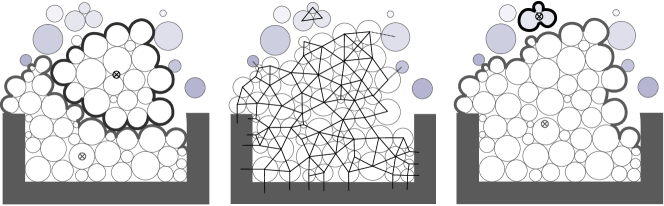
Figure 3: Illustration the merge procedure: detection of contacts involving two aggregates and 11 free particles (left), identification of two disconnected networks fulfilling the merge conditions (middle), creating two new aggregates (right). The colour intensity codes velocity.

3.2 Split

There are a number of ways to predict if and how the reduced model should be refined by splitting the rigid aggregates into smaller aggregates and free particles. One strategy is to rely on contact events, that is, trigger splitting by impacts and separations. Another strategy is to do a fast trial solve in the background, using a more resolved model, and decide splitting from the outcome. A third, more heuristic approach, is to add split sensors in the system. The placement of the sensors can be made automatic, after a posteriori analysis of previous simulations of the same or similar system, or manually, based on experience or perspicacity. The split methods can also be used in combination with each other. The different methods, illustrated in Fig. 4, are outlined in further detail below and tested in numerical experiments. Observe that the split process does not affect on the total mass or momentum.

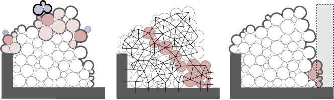
Figure 4: Illustration of different split methods: contact split (left), trial solve split (middle) and sensor split (right). Blue particles have impacting or separating contacts. Red particles are aggregate particles that are to be split from the aggregate. The dashed grey box represent a split sensor.

The process of splitting an aggregate is the same irrespective of the method used for the prediction. The split particles are made dynamic and the new aggregates are determined and created as in the merge process, by analysing the contact network after removing the split particles and applying Eq. (6)-(10).

3.2.1 Contact split

Contacts are either impacting, continuous or separating depending on the sign and magnitude of the relative velocity. For each contact $n\in{\mathcal{N}}_{\text{c}}$, between particle $a$ and aggregate $A$, the following conditions for normal, tangential and rolling motion are tested

$$\textbf{G}^{(n)}_{\text{n}[aA]}\textbf{v} \notin [-\xi^{\text{i-c}}_{\text{n}v},\xi^{\text{s-c}}_{\text{n}v}],$$ (29)

$$\textbf{G}^{(n)}_{\text{t}[aA]}\textbf{v} \notin [-\xi^{\text{c}}_{\text{t}v},\xi^{\text{c}}_{\text{t}v}],$$ (30)

$$\textbf{G}^{(n)}_{\text{r}[aA]}\textbf{v} \notin [-\xi^{\text{c}}_{\text{r}v},\xi^{\text{c}}_{\text{r}v}],$$ (31)

with impact split threshold denoted with i-c and separation split threshold with s-c. If either of the relative contact velocities are found to be outside the valid domain, the aggregate is refined by splitting off particles at the contact node $n$. The split may be applied to some split depth ${N}_{\text{c-spl}}\in\mathbb{N}$ along the contact network from the impact (or separation) node in order to capture shock propagation phenomena. Observe that the split action is merely a redefinition of which particles are free and which are kinematically bound to aggregate bodies. This does not immediately alter the position or velocity of any particle. The split is then proceeded with solving the impact stage MCP and the continuous stage MCP, see Algorithm 1. There is therefore no risk, other than unnecessary computations, of splitting too many particles. These will be merged back with the aggregate if the merge condition is fulfilled after solving the impact and continuous MCP. The numerical experiments presented in this paper is limited to splitting aggregate particles that are triggered by impact or separation directly and their contact neighbours, i.e., ${N}_{\text{c-spl}}=2$. Impacts between two aggregates are treated the same way.

3.2.2 Trial solve split

A trial solver is run in the background to estimate the dynamics of the full system. The background system state is initialized by projecting the reduced sub-space system back to the full resolution space of Eq. (11)-(13). The purpose of the background solve is not to do precise integration of the particle positions and velocities but to provide sufficient estimate for if and how to split rigid aggregates. Assuming that the state of the reduced system from previous timestep was a good approximation of the full system it is conjectured that doing a PGS solve of the full system MCP with low number of iterations $N_{\text{it}}^{\text{tr}}$ will suffice for this, although the error of such a simulation would increase rapidly over time. Other alternatives can be imagined, e.g., doing the background computation using other solvers or on a partially resolved system. The background trial solution is tested for the following conditions for relative velocity of each contact $n\in{\mathcal{N}}_{\text{c}}$

$$\textbf{G}^{(n)}_{\text{n}[aA]}\textbf{v} \notin [-\xi^{\text{i-tr}}_{\text{n}v},\xi^{\text{s-tr}}_{\text{n}v}],$$ (32)

$$\textbf{G}^{(n)}_{\text{t}[aA]}\textbf{v} \notin [-\xi^{\text{tr}}_{\text{t}v},\xi^{\text{tr}}_{\text{t}v}],$$ (33)

$$\textbf{G}^{(n)}_{\text{r}[aA]}\textbf{v} \notin [-\xi^{\text{tr}}_{\text{r}v},\xi^{\text{tr}}_{\text{r}v}],$$ (34)

and the following conditions for force and torque balance are tested separately for each aggregated particle $a$

$$\frac{|\vec{\textbf{f}}_{\text{e}[a]}-\textbf{G}^{T}_{f[a]}\bm{\lambda}|}{|\vec{\textbf{f}}_{\text{e}[a]}|+|\textbf{G}^{T}_{f[a]}\bm{\lambda}|} < \xi^{\text{tr}}_{f},$$ (35)

$$\frac{|\vec{\bm{\tau}}_{\text{e}[a]}-\textbf{G}^{T}_{\tau[a]}\bm{\lambda}|}{|\vec{\bm{\tau}}_{\text{e}[a]}|+|\textbf{G}^{T}_{\tau[a]}\lambda|} < \xi^{\text{tr}}_{\tau}.$$ (36)

where $\textbf{G}^{T}_{f[a]}\bm{\lambda}$ and $\textbf{G}^{T}_{\tau[a]}\bm{\lambda}$ are the force and torque components of the sum of generalized contact forces acting on particle $a$, $\textbf{G}^{T}_{[a]}\bm{\lambda}=\sum_{b\in\mathcal{N}_{\text{c}}^{a}}\textbf{G}^{T}_{[ab]}\bm{\lambda}$. The Jacobians are the blocks for linear and rotational degrees of freedom $\textbf{G}^{T}_{[a]}=[\textbf{G}^{T}_{f[a]},\textbf{G}^{T}_{\tau[a]}]$. Observe that $\bm{\lambda}$ has replaced $\tfrac{\eta}{\varepsilon}\textbf{g}$ in the force balance condition (25). This is a stronger test as it can detect also acceleration due to impulse force propagation through the system that has not yet resulted in relative contact velocity or particle displacements. The particles that are indicated by the tests are eliminated from the aggregate body and activated as a dynamic particle. In the numerical implementation a small perturbation is added to the denominators to avoid numerical round-off errors.

3.2.3 Sensor split

The split sensor is simply a geometrical shape that triggers model refinement of aggregate bodies that overlap with the sensor geometry. The splitting is applied only to the aggregate particles that overlap the sensor. Observe that the sensors are physically transparent and do not produce any contact forces. Split sensors is a useful tool for when it can be anticipated where model refinement is required without doing a background trial solve. The sensor must be given a size, shape and position, either manually or automated based on data from simulations, models or experiments.

4 Numerical experiments

The described method for adaptive model order reduction is investigated in numerical experiments. The test systems are a conveyor with a continuous formation of a pile on one end and discharge at the other end, a granular collapse and granular flow in a slowly rotating drum. The granular dynamics from using model reduction is compared with reference simulations run in full resolution. The achieved model order reduction level, $h(t)=1-\tilde{N}_{\text{p}}(t)/N_{\text{p}}$, is monitored. The tests are selected to represent different types of flow and transitions between static and dynamic states. Model reduction can be expected to work well for the formation of piles where the dynamics mainly occur in the surface layers. For granular discharge and collapse there is high risk of approximation errors by to predict when and where the aggregate should split and flow. In a slowly rotating drum the granular flow separate in one zone of rapid flow (shear zone) on top of a plug zone that co-rotate with the drum. The plug zone does not rotate as an ideal rigid body, however, but has a small shear creep [20] that may render model reduction into rigid aggregates problematic. The simulations are made using the simulation software AgX Dynamics [21] with a prototype implementation of the adaptive model reduction algorithms in Lua scripts [22]. The prototype implementation is not optimized for speed and memory and the tests are therefore limited to relatively small systems ranging between ${N}_{\text{p}}=4-90\cdot 10^{3}$ particles. The model and NDEM simulation parameters are listed in Table 1 and the adaptive model order reduction parameters in Table 2. A linear contact model is used, with normal stiffness ${k}_{\text{n}}$, and may easily be replaced by the nonlinear Hertz contact law. Mono-sized spherical particles are used, except in the granular collapse where bi-disperse spheres are used. Gravity acceleration is $9.81$ m/s². Videos from simulations are available as supplementary material at http://umit.cs.umu.se/modelreduction/.

Table 1: Model and NDEM parameters

$d$	$13,10$ mm
$\rho$	$3700$ kg/m3
${k}_{\text{n}}$	$3$ kN/m
$e$	$0.18$
${\mu}_{\text{t}}$	$0.91$
${\mu}_{\text{r}}$	$0.32$
$\Delta t$	$5$ ms
${N}_{\text{p}}$	$4-90\cdot 10^{3}$
${N}_{\text{it}}$	$150$
$N_{\text{it}}^{\text{ref}}$	$150,500$

Table 2: Model order reduction parameters

parameter	value
$\xi_{\text{n}v}^{\text{i-mrg}}$	$2.5$ mm/s
$\xi_{\text{n}v}^{\text{s-mrg}}$	$2.5$ mm/s
$\xi_{\text{t}v}^{\text{mrg}}$	$2.5$ mm/s
$\xi_{\text{r}v}^{\text{mrg}}$	$0.5$ rad/s
$\xi_{\text{n}a}^{\text{i-mrg}}$	$5$ m/s2
$\xi_{\text{n}a}^{\text{s-mrg}}$	$5$ m/s2
$\xi_{\text{t}a}^{\text{mrg}}$	$5$ m/s2
$\xi_{\text{r}a}^{\text{mrg}}$	$\infty$ rad/s
${N}_{\text{c-spl}}$	$2$
$\xi^{\text{i-c}}_{\text{n}v}$	$0.15$ m/s
$\xi^{\text{s-c}}_{\text{n}v}$	$\infty$ m/s
$\xi^{\text{c}}_{\text{t}v}$	$0.15$ m/s
$\xi^{\text{c}}_{\text{r}v}$	$\infty$ rad/s
$N_{\text{it}}^{\text{tr}}$	$50,100$
$\xi^{\text{i-tr}}_{\text{n}v}$	$2.6$ m/s
$\xi^{\text{s-tr}}_{\text{n}v}$	$0.26$ m/s
$\xi^{\text{tr}}_{\text{t}v}$	$0.26$ m/s
$\xi^{\text{tr}}_{\text{r}v}$	$\infty$ rad/s
$\xi^{\text{tr}}_{f}$	$0.15,0.25$
$\xi^{\text{tr}}_{\tau}$	$\infty$

The pile formation is performed by emitting particles at a rate of $1000$ s^-1 from $0.1$ m above a planar conveyor surface moving with horizontal speed $0.1$ m/s. The emitter surface is $15d\times 4d$, in which the particle positions are chosen randomly. The particles quickly come to relative rest on the conveyor, forming an elongated pile, roughly $10d$ high and with static angle repose $\theta_{\text{conv}}$. The angle of repose is computed as the average inclination of the pile surface defined by the surface particles in the mid section of the conveyor, neglecting particles resting directly on the conveyor surface, see Fig. 5. The discharge take place on the end of the $50d$ long conveyor, where the material loose support and flow over the edge. The cross sectional flow distribution in the horizontal plane is measured $15d$ below the conveying surface and the geometric centre of the flow is computed, $({x}_{\text{c}},{y}_{\text{c}})$. The result is time averaged over $6$ s. The conveyor system involves $90\cdot 10^{3}$ particles when the conveyor is filled.

The granular collapse test is made with $4000$ particles emitted randomly from above into a frictionless cubic container with side length $15d$. The particles are left to comte to rest before model reduction is applied. One side-wall is raised quickly and the particles are left to collapse by the new and unstable force configuration. Since the side walls are frictionless the raising of the wall does not disturb the particles other than the change in the confining pressure. The granular collapse last for about $0.7$ s, after which the particle have come to rest in a semi-pile with well-defined angle of repose, ${\theta}_{\text{collapse}}$. The evolution of the angle of repose is tracked by estimating the motion of the plane defined by the particles on the top surface of the granular cube, discarding any particles that disconnect from the main contact network. Images from simulations are shown in Fig. 6.

The rotating drum has diameter $D=40d$, width $w=7d$ and is run with angular velocity $\Omega=0.5$ rad/s. The corresponding dimensionless Froude number is $\text{Fr}\equiv D\Omega^{2}/2g\approx 0.01$, which is in the dense rolling flow regime. The side walls are frictionless while the cylinder surface has the sama friction as between particles. A slow dense nearly stationary flow with ${N}_{\text{p}}=4864$ particles is established within one drum revolution without applying model reduction and starting from a regular particle distribution. An image from the simulations is shown in Fig. 7. The particles have bi-disperse size distribution $d_{1}=13$ mm and $d_{2}=10$ mm. The mass distribution and cross sectional flow velocity field are measured and the dynamic angle of repose, $\theta_{\text{drum}}$, is computed by tracking the a $D/2$ wide section of the surface around the drum centre. When using sensor split, the sensor is placed around the estimated lift height.

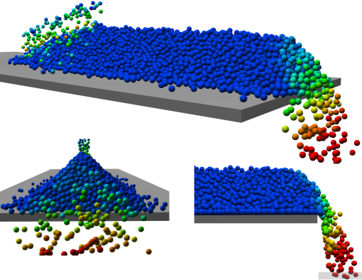
Figure 5: Simulation test for pile formation and discharge on the ends of a conveyor. The colour is coded by particle velocity relative to the conveyor speed and ranges from $0$ (blue) to $1.5$ m/s or above (red).

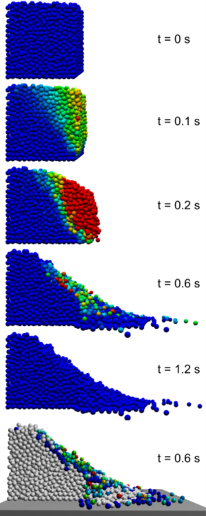
Figure 6: Image sequence from granular collapse. The colour is coded by particle velocity ranging from $0$ (blue) to $0.5$ m/s or above (red). The top five figures are reference simulation and the bottom figure uses model reduction with background trial solve split.

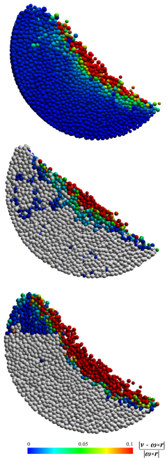
Figure 7: Image from drum flow simulation. The colour is coded by particle relative velocity to rigid co-motion with the drum, ranging from $0$ (blue) to $10\%$ or above (red). The top figure show the reference simulation, the middle one uses model reduction with background trial solve split and the bottom one contact event and sensor split.

5 Results

The simulation results are labeled either ref-500, ref-150, cs-150, tr-150-50-f or ctr-150-50-fv, where the first prefix refer to reference simulation or the method for model reduction, the first number is the number or PGS iterations and the second number is the number iterations in the background trial solver (tr) using force balance condition only (f) or in conjunction with velocity condition (fv). It was found that separation splitting was very sensitive to parameters and typically lead to either a propagation of splitting over the entire aggregates or not enough splitting. Therefore it is not applied, i.e., $\xi^{\text{s-c}}_{\text{n}v}=\infty$, and contact splitting need to be combined with either sensors (cs) or with trial splitting (ctr). The results are summarized in Table 3.

Table 3: Simulation results

	ref-500	ref-150	cs-150	tr-150-50-f	tr-150-50-fv
${\theta}_{\text{conv}}$	$41.5\pm 0.7^{\circ}$	$40.6\pm 0.5^{\circ}$	$40.3\pm 0.8^{\circ}$
$h_{\text{conv}}^{\text{mean}}$	$0$ %	$0$ %	$85$ %
${\theta}_{\text{collapse}}$	$36^{\circ}$	$30^{\circ}$		$38^{\circ}$	$34^{\circ}$
$h_{\text{collapse}}$	$0$ %	$0$ %		$50-100$ %	$50-100$ %
${\theta}_{\text{drum}}$	$44\pm 3^{\circ}$	$43\pm 2^{\circ}$	$49\pm 5^{\circ}$	$44\pm 3^{\circ}$	$45\pm 2^{\circ}$
$h_{\text{drum}}^{\text{mean}}$	$0$ %	$0$ %	$70\pm 10$ %	$40\pm 10$ %	$40\pm 10$ %

The resting angle of repose of the pile formed on the conveying surface is found to be $40.3\pm 0.8^{\circ}$ using contact splitting. This is in good agreement with the references $41.5\pm 0.7^{\circ}$ for ${N}_{\text{it}}=500$ and $40.6\pm 0.5^{\circ}$ for ${N}_{\text{it}}=150$. The discharge flow at the end of the conveyor is presented in Fig. 8. The cross-sectional flow distribution is very similar in the three simulations. The model order reduction level was steady around $h=85$ % during the simulation.

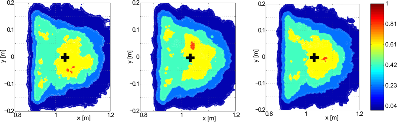
Figure 8: The discharge flow through a horizontal cross-section beneath the end of the conveyor. The contour plots show the accumulated particles distribution from the reference simulations ${N}_{\text{it}}=500$ (left), ${N}_{\text{it}}=150$ (right) and simulation with model reduction using contact and sensor splitting (right). The crosses mark the geometric centre of the particle distributions.

The distribution of particles after the granular collapse are displayed in Fig. 9. The positions are measured at time $t=2$ s. The angle of repose, ${\theta}_{\text{collapse}}$, of the ${N}_{\text{it}}=500$ reference pile is $36.2^{\circ}$, to be compared with $29.9^{\circ}$ for the ${N}_{\text{it}}=150$ reference and $37.5^{\circ}$ and $34^{\circ}$ for model reduction with background trial solve with force (f) and force and velocity (fv) split conditions, respectively.

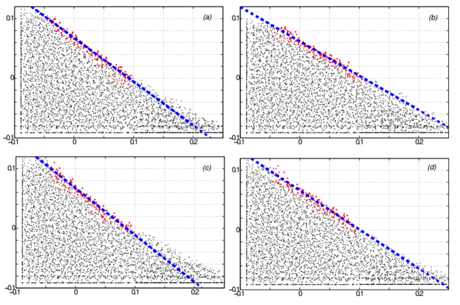
Figure 9: The final particle distribution in the granular collapse simulations: (a) ${N}_{\text{it}}=500$ reference; (b) ${N}_{\text{it}}=150$ reference; (c) model reduction tr-15-50-f; (d) model reduction tr-15-50-fv. The blue line indicate the angle of repose computed from the surface defined by the red particles.

The evolution of the inclination angle of the top surface of the collapsing cube is found in Fig. 10. The initial collapse is similar in all the simulations except the tr-150-50-f that evolve somewhat slower initially. The ${N}_{\text{it}}=150$ reference simulation reach as highest $34^{\circ}$ and then decrease gradually due to insufficient sliding and rolling resistance with that number of iterations. The model reduction simulation become rigid at its maximum angle and fail to resolve the final relaxation of the slope through small avalanches, that are present in the ${N}_{\text{it}}=500$ reference simulation. The combination of contact split and background trial split did not resolve this.

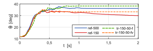
Figure 10: Evolution of the top surface angle during granular collapse.

The evolution of the model reduction level is found in Fig. 11. In the background trial solve split simulation the reduction level varies between $50$ and $100$ %. This is close to the theoretical maximum for the given thresholds, found by analysing the ${N}_{\text{it}}=500$ reference simulation.

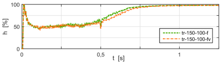
Figure 11: Model reduction level as function of time in granular collapse.

Sample states from model reduction of drum flow simulations are presented in Fig. 7. The evolution of the dynamic angle of repose is found in Fig. 12.

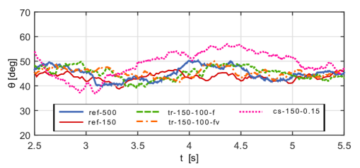
Figure 12: Evolution of the dynamic angle of repose in the rotating drum.

The time-averaged angle of repose for the reference ${N}_{\text{it}}=500$ is ${\theta}_{\text{drum}}=44\pm 3^{\circ}$. The background trial solve split method produces a flow with angle $44\pm 3^{\circ}$ while the contact plus sensor split methods produces a flow with angle $49\pm 5^{\circ}$ and with notable artefacts appearing as structures with angle much larger than the angle of repose and high lifting of material in the drum. This is also the reason for the bigger variation on the averaged angle of repose. No thresholds were found for the contact split method alone that showed any significant model reduction but did not produce large approximation errors (overly rigid). No thresholds were found for the contact split method alone that showed any significant model reduction but did not produce large approximation errors (overly rigid). The model reduction level over time is presented in Fig. 13. For the contact method plus sensor split method it varies between $50\--75$ %. The background trial solve split oscillate between $25$ and $50$%. No parameters were found that gave higher level of reduction without increase of artifacts in the dynamics.

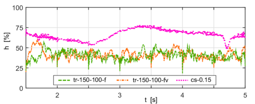
Figure 13: Model reduction level $h$ as function of time in the rotating drum.

6 Computational acceleration

The potential computational acceleration of using model order reduction in NDEM simulations is estimated and discussed in this section. The time required for simulating ${t}_{\text{real}}$ seconds of evolution is the product of the number of time steps and the computational time for each step

$${t}_{\text{comp}}=\frac{{t}_{\text{real}}}{\Delta t}\cdot\left[{t}_{\text{coll}}+{t}_{\text{mod}}+{t}_{\text{solve}}\right]$$ (37)

with time serially separated in collision detection, ${t}_{\text{coll}}$, model order reduction, ${t}_{\text{mod}}$ and solver time, ${t}_{\text{solve}}$. We define the computational speed-up from model order reduction as $S\equiv t^{0}_{\text{comp}}/{t}_{\text{comp}}(h)$, where $t^{0}_{\text{comp}}$ refer to a simulation of the fully resolved system without adaptive model reduction, while ${t}_{\text{comp}}(h)$ is the time for a simulation with model reduction level $h$. It is characteristic for NDEM simulations that ${t}_{\text{solve}}\gg{t}_{\text{coll}}$, e.g., 88% of the total time was reported in [23]. We therefore discard collision detection time from here on. When using PGS, the solve time can be estimated by ${t}_{\text{solve}}={K}_{\text{cpu}}\cdot{N}_{\text{c}}\cdot{N}_{\text{it}}/S_{\parallel}$, where ${K}_{\text{cpu}}$ is the computational time for doing a single contact constraint solve, ${N}_{\text{c}}\sim{n}_{\text{p}}{\tilde{N}}_{\text{p}}$ is the number of contact constraints assuming on average $2{n}_{\text{p}}$ contacts per particle, and $S_{\parallel}({N}_{\text{cpu}})$ is the parallel speed-up of ${N}_{\text{cpu}}$ cores. Given a spatial error tolerance, $\epsilon$, the required number of iterations scale with the number of particles as ${N}_{\text{it}}=c{\tilde{N}}_{\text{p}}^{\gamma}/\epsilon$ [19], for constant $c\approx 0.1$ and exponent $\gamma=1/{n}_{\text{D}}$ that depend on the whether the system is close to a linear column (${n}_{\text{D}}=1$) , 2D plane (${n}_{\text{D}}=2$) or a 3D volumetric system (${n}_{\text{D}}=3$). The solve time can thus be written

$${t}_{\text{solve}}(h)=c{K}_{\text{cpu}}\left[(1-h)N_{\text{p}}\right]^{1+\gamma}/\epsilon S_{\parallel}.$$ (38)

The computational overhead for doing merge and refinement using contact or sensor based splitting do not involve more than one pass through the contact network. The computational time can thus be estimated by ${t}_{\text{mod}}=\alpha{K}_{\text{cpu}}{n}_{\text{p}}{N}_{\text{p}}/S_{\parallel}$ for some constant $\alpha<1$, since the operations do not involve solving the local contact problem. This imply the following speed-up

$$S\approx\frac{1}{\alpha{N}_{\text{p}}^{-\gamma}+(1-h)^{1+\gamma}}.$$ (39)

Using background trial solve split for model reduction is more demanding. If a PGS background solve can be limited to fraction $\beta<1$ of the full system and run with a larger error tolerance, $\epsilon_{\text{mod}}>\epsilon$, the computational overhead can be estimated to ${t}_{\text{mod}}=c{K}_{\text{cpu}}\left[\beta N_{\text{p}}\right]^{1+\gamma}/\epsilon_{\text{mod}}S_{\parallel}$ and the speed-up become

$$S\approx\frac{1}{\beta^{1+\gamma}\cdot\epsilon/\epsilon_{\text{mod}}+(1-h)^{1+\gamma}}.$$ (40)

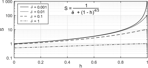
Figure 14: The computational speed-up depending on model reduction level and computational overhead.

The computational speed-up, depending on model reduction level $h$ and overhead factor $\delta=\alpha{N}_{\text{p}}^{-\gamma}$ or $\delta=\beta^{1+\gamma}\cdot\epsilon/\epsilon_{\text{mod}}$, is plotted in Fig. 14 for the case of 3D volumetric systems ($\gamma=1/3$). A significant speed-up of a factor $5$ can be achived even at the modest model reduction level $h=0.7$. The speed-up can reach up to $50$ at $h=0.95$ and overhead $\delta=0.01$. The potential speed-up is lost almost entirely if the computational overhead cannot be made lower than $\delta=0.1$. This should be easy to accomplish in the case of contact and sensor based splitting, especially for large systems where $\delta\propto{N}_{\text{p}}^{-\gamma}$. Achieving a significant speed-up from background trial solve split thus relies on $\beta^{1+\gamma}\cdot\epsilon/\epsilon_{\text{mod}}\lesssim 0.1$. This can be reached if it is sufficient to apply background solve on a fraction of $\beta=0.2$ of the full system or use a background error tolerance $\epsilon_{\text{mod}}=10\cdot\epsilon$. Combining the two possibilities, an overhead of about $0.1$ can be reached by $\beta=0.5$ and $\epsilon_{\text{mod}}=4\cdot\epsilon$. The prototype implementation do not scale sufficiently well for large systems to verify these estimates. To ease prototyping and experimentation with different algorithms and parameters for model order reduction these routines were implemented in a Lua scripting framework which lead to an unnecessary amount of data copying of states.

7 Conclusion and discussion

A method for adaptive model order reduction for nonsmooth discrete element simulation has been developed and analysed. In the reduced model rigid aggregate bodies are substituted for collections of contacting particles collectively moving as rigid bodies. Conditions for model reduction and refinement are derived from a model approximation error. The scaling analysis show that the computational performance may be increased by $5-50$ times for a model reduction level between $70-95$ % given that the computational overhead do not exceed the given scaling conditions. The method is highly applicable for granular systems with large regions in resting or rigidly co-moving state over long periods. It is less efficient and harder to parametrize for systems with sudden and frequent transitions between rigid to liquid or gaseous regime and it is directly inappropriate for systems dominated by shear motion. Furthermore, the presented method is fully compatible with rigid multibody dynamics and can support particles merging with articulated mechanisms, such as the excavator in Fig. 1.

A number of observations were made in the numerical experiments. When doing model refinement based on contact events, it is in general insufficient to split only particles that are impacted directly. The refinement typically need to propagate further into the contact network. The refinement depth $N^{\text{spl}}_{c}=2$ was used in the experiments. Refinement based on contact separation events was found to be particularly difficult to parametrize and was eventually not used at all. Small changes in the separation threshold easily altered the behaviour from non-responding to splitting propagating throughout the contact network. As an effect, contact event based refinement is not reliable for simulating quasi-stable configurations and gravity driven flow. In the absence of impacts, rigid aggregates remain rigid indefinitely. Split sensors can be used to remedy this when there is knowledge on where to place such sensors to guarantee refinement.

When using background trial solve it was found that the force balance condition alone give reliable prediction for model refinement. No improvement was found by adding torque balance or contact velocity conditions. Using background solve, velocity condition alone led to higher fluctuations in the model order reduction level than using both force and velocity conditions.

To increase the applicability of adaptive model order reduction for discrete element methods further, the reduced model need to be extended beyond rigid aggregates to elastic and shearing modes. The application of model order reduction to conventional smooth DEM is also an interesting question to address.

Appendix

A. Numerical integration of NDEM

The numerical time integration scheme is based on the SPOOK stepper [18] derived from discrete variational principle for the augmented system $(\textbf{x},\textbf{v},\bm{\lambda},\dot{\bm{\lambda}})$ and applying a semi-implicit discretization. The stepper is linearly stable and $\mathcal{O}(\Delta t^{2})$ accurate for constraint violations [18]. Stepping the system position and velocity, $(\textbf{x}_{i},\textbf{v}_{i})\to(\textbf{x}_{i+1},\textbf{v}_{i+1})$, from time $t_{i}$ to $t_{i+1}=t_{i}+\Delta t$ involve solving a mixed complementarity problem (MCP) [24]. For a NDEM system the MCP take the following form

$$\begin{array}[c]{c}\textbf{H}\textbf{z}+\textbf{b}=\textbf{w}_{l}-\textbf{w}_{u}\\ \mbox{\scriptsize$0\leq\textbf{z}-\textbf{l}\perp\textbf{w}_{l}\geq 0$ }\\ \mbox{\scriptsize$0\leq\textbf{u}-\textbf{z}\perp\textbf{w}_{u}\geq 0$ }\end{array}$$ (41)

where

$$\textbf{H}=\left[\begin{array}[c]{cccc}\textbf{M}&-{\textbf{G}}_{\text{n}}^{\text{T}}&-{\textbf{G}}_{\text{t}}^{\text{T}}&-{\textbf{G}}_{\text{r}}^{\text{T}}\\ {\textbf{G}}_{\text{n}}&{\bm{\Sigma}}_{\text{n}}&0&0\\ {\textbf{G}}_{\text{t}}&0&{\bm{\Sigma}}_{\text{t}}&0\\ {\textbf{G}}_{\text{r}}&0&0&{\bm{\Sigma}}_{\text{r}}\\ \end{array}\right],$$ (42)

$$\textbf{z}=\begin{bmatrix}{\textbf{v}_{i+1}}\\ \bm{\lambda}_{\text{n},i+1}\\ \bm{\lambda}_{\text{t},i+1}\\ \bm{\lambda}_{\text{r},i+1}\end{bmatrix},\ \ \textbf{b}=\begin{bmatrix}{-\textbf{M}\textbf{v}_{i}-\Delta t\textbf{M}^{-1}{\textbf{f}}_{\text{ext}}}\\ \tfrac{4}{\Delta t}{\bm{\Upsilon}}_{\text{n}}{\textbf{g}}_{\text{n}}-{\bm{\Upsilon}}_{\text{n}}{\textbf{G}}_{\text{n}}\textbf{v}_{i}\\ {0}\\ {0}\end{bmatrix},$$ (43)

and the solution vector z contains the new velocities and the Lagrange multipliers $\bm{\lambda}_{\text{n}}$, $\bm{\lambda}_{\text{t}}$ and $\bm{\lambda}_{\text{r}}$. For notational convenience, a factor $\Delta t$ has been absorbed in the multipliers such that the constraint force reads $\textbf{G}^{T}\bm{\lambda}/\Delta t$. The upper and lower limits, $u$ and $l$ in Eq. (41), follow from Signorini-Coulomb and rolling resistance law with the friction and rolling resistance coefficients ${\mu}_{\text{t}}$ and ${\mu}_{\text{r}}$. Since the limits depend on the solution this is a partially nonlinear complementarity problem. $w_{l}$ and $w_{u}$ are temporary slack variables. Each contact $n$ between body $a$ and $b$ add contributions to the constraint vector and normal, friction and rolling Jacobians according to

$$g_{(n)} = \vec{\textbf{n}}_{(n)}^{\text{T}}(\vec{\textbf{x}}_{[a]}+\vec{\textbf{d}}^{(n)}_{[a]}-\vec{\textbf{x}}_{[b]}-\vec{\textbf{d}}^{(n)}_{[b]})^{{e}_{\text{H}}}_{(\alpha)},$$

$$\textbf{G}_{\text{n}[a]}^{(n)} = {e}_{\text{H}}g^{{e}_{\text{H}}-1}_{(\alpha)}\left[\begin{array}[c]{cc}-\vec{\textbf{n}}_{(n)}^{{\text{T}}}&\ \ -(\vec{\textbf{d}}^{(n)}_{[a]}\times\vec{\textbf{n}}_{(n)})^{\text{T}}\end{array}\right],$$ (45)

$$\textbf{G}_{\text{n}[b]}^{(n)} = {e}_{\text{H}}g^{{e}_{\text{H}}-1}_{(\alpha)}\left[\begin{array}[c]{cc}\vec{\textbf{n}}_{(n)}^{{\text{T}}}&\ \ (\vec{\textbf{d}}^{(n)}_{[b]}\times\vec{\textbf{n}}_{(n)})^{\text{T}}\end{array}\right],$$ (47)

$$\textbf{G}_{\text{t}[a]}^{(n)} = \left[\begin{array}[c]{cc}-\vec{\textbf{t}}^{(n){\text{T}}}_{1}&\ \ -(\vec{\textbf{d}}^{(n)}_{[a]}\times\vec{\textbf{t}}^{(n)}_{1})^{\text{T}}\\ -\vec{\textbf{t}}^{(n){\text{T}}}_{2}&\ \ -(\vec{\textbf{d}}^{(n)}_{[a]}\times\vec{\textbf{t}}^{(n)}_{2})^{\text{T}}\end{array}\right],$$ (50)

$$\textbf{G}_{\text{t}[b]}^{(n)} = \left[\begin{array}[c]{cc}\vec{\textbf{t}}^{(n){\text{T}}}_{1}&\ \ (\vec{\textbf{d}}^{(n)}_{[b]}\times\vec{\textbf{t}}^{(n)}_{1})^{\text{T}}\\ \vec{\textbf{t}}^{(n){\text{T}}}_{2}&\ \ (\vec{\textbf{d}}^{(n)}_{[b]}\times\vec{\textbf{t}}^{(n)}_{2})^{\text{T}}\end{array}\right],$$ (53)

$$\textbf{G}_{\text{r}[a]}^{(n)} = \left[\begin{array}[c]{cccc}\mathbf{0}_{1\times 3}&\ \vec{\textbf{t}}^{(n){\text{T}}}_{1}&\ \ \mathbf{0}_{1\times 3}&-\vec{\textbf{t}}^{(n){\text{T}}}_{1}\\ \mathbf{0}_{1\times 3}&\ \vec{\textbf{t}}^{(n){\text{T}}}_{2}&\ \ \mathbf{0}_{1\times 3}&-\vec{\textbf{t}}^{(n){\text{T}}}_{2}\\ \mathbf{0}_{1\times 3}&\ \vec{\textbf{n}}^{(n){\text{T}}}&\ \ \mathbf{0}_{1\times 3}&-\vec{\textbf{n}}^{(n){\text{T}}}\\ \end{array}\right],$$ (57)

$$\textbf{G}_{\text{r}[b]}^{(n)} = \left[\begin{array}[c]{cccc}\mathbf{0}_{1\times 3}&\ \ -\vec{\textbf{t}}^{(n){\text{T}}}_{1}&\ \ \mathbf{0}_{1\times 3}&\vec{\textbf{t}}^{(n){\text{T}}}_{1}\\ \mathbf{0}_{1\times 3}&\ \ -\vec{\textbf{t}}^{(n){\text{T}}}_{2}&\ \ \mathbf{0}_{1\times 3}&\vec{\textbf{t}}^{(n){\text{T}}}_{2}\\ \mathbf{0}_{1\times 3}&\ \ -\textbf{n}^{(n){\text{T}}}&\ \ \mathbf{0}_{1\times 3}&\vec{\textbf{n}}^{(n){\text{T}}}\\ \end{array}\right],$$ (61)

where $\vec{\textbf{d}}^{(n)}_{[a]}$ and $\vec{\textbf{d}}^{(n)}_{[b]}$ are the positions of the contact point $n$ relative to the particle positions $\vec{\textbf{x}}_{[a]}$ and $\vec{\textbf{x}}_{[b]}$. The orthonormal contact normal and tangent vectors are $\vec{\textbf{n}}_{(n)}$, $\vec{\textbf{t}}_{(n)_{1}}$ and $\vec{\textbf{t}}_{(n)_{2}}$. For linear contact model ${e}_{\text{H}}=1$ and for the nonlinear Hertz-Mindlin model ${e}_{\text{H}}=5/4$. The diagonal matrices ${\bm{\Sigma}}_{\text{n}}$, ${\bm{\Sigma}}_{\text{t}}$ , ${\bm{\Sigma}}_{\text{r}}$ and ${\bm{\Upsilon}}_{\text{n}}$ contain the contact material parameters and are as follows

$${\bm{\Sigma}}_{\text{n}} = \frac{4}{\Delta t^{2}}\frac{{\varepsilon}_{\text{n}}}{1+4\tfrac{{\tau}_{\text{n}}}{\Delta t}}\bm{1}_{N_{c}\times N_{c}},$$

$${\bm{\Sigma}}_{\text{t}} = \frac{{\gamma}_{\text{t}}}{\Delta t}\bm{1}_{2N_{c}\times 2N_{c}},$$

$${\bm{\Sigma}}_{\text{r}} = \frac{{\gamma}_{\text{r}}}{\Delta t}\bm{1}_{3N_{c}\times 3N_{c}},$$ (62)

$${\bm{\Upsilon}}_{\text{n}} = \frac{1}{1+4\tfrac{{\tau}_{\text{n}}}{\Delta t}}\bm{1}_{N_{c}\times N_{c}}.$$

The MCP parameters map to DEM material parameters by ${\varepsilon}_{\text{n}}={e}_{\text{\tiny H}}/{k}_{\text{n}}$, ${\gamma}_{\text{n}}^{-1}={k}_{\text{n}}c/e^{2}_{\text{\tiny H}}$ and ${\tau}_{\text{n}}=\max({n}_{\text{s}}\Delta t,{\varepsilon}_{\text{n}}/{\gamma}_{\text{n}})$, with elastic stiffness coefficient ${k}_{\text{n}}$ and viscosity $c$. For the Hertz-Mindlin contact law, ${k}_{\text{n}}={e}_{\text{\tiny H}}E\sqrt{r^{*}}/3(1-\nu^{2})$ where $r^{*}=(r_{a}+r_{b})/r_{a}r_{b}$ is the effective radius, $E$ is the Young’s modulus and $\nu$ is the Poisson ratio. For small relative contact velocities the normal force approximates $\textbf{G}_{\text{n}}^{(n){\text{T}}}\bm{\lambda}_{\text{n}}^{(n)}\approx\varepsilon_{\text{n}}^{-1}\textbf{G}_{\text{n}}^{(n){\text{T}}}\textbf{g}_{\text{n}}^{(n)}=\pm{k}_{\text{n}}\left[{\textbf{g}}_{\text{n}}^{2{e}_{\text{\tiny H}}-1}+c{\textbf{g}}_{\text{n}}^{2({e}_{\text{\tiny H}}-1)}\dot{g}_{\text{n}}\right]\bm{n}$. High ingoing velocities are treated as impacts and this is done post facto. After stepping the velocities and positions an impact stage follows. This include solving a MCP similar to Eq. (41) but with the Newton impact law, ${\textbf{G}}_{\text{n}}^{(n)}\textbf{v}_{+}=-e{\textbf{G}}_{\text{n}}^{(n)}\textbf{v}_{-}$, replacing the normal constraints for the contacts with normal velocity larger than an impact velocity threshold ${v}_{\text{imp}}$. The remaining constraints are maintained by imposing $\textbf{G}^{(n)}\textbf{v}_{+}=0$. This can be expressed by a matrix multiplication ${\textbf{G}}_{\text{n}}\textbf{v}_{+}=-\textbf{E}{\textbf{G}}_{\text{n}}\textbf{v}_{-}$, where the diagonal matrix E values alternate between $e$ and $0$ for impacting and resting contacts, respectively. The MCP is solved using a projected Gauss-Seidel (PGS) algorithm, as described in Ref. [19]. The algorithm is listed in Algorithm 2. The NDEM method with PGS solver is implemented in the software AgX Dynamics [21]. In the present study ${\gamma}_{\text{t}}={\gamma}_{\text{r}}=10^{-6}$, ${n}_{\text{s}}=2$ was used and a linear contact model, ${e}_{\text{\tiny H}}=1$, for consistency with contacts between elementary rigid bodies and aggregate bodies, for which linear contact constraints are default in AgX.

Algorithm 2 PGS solver for the MCP

if impact stage then

     ${\textbf{b}}_{\text{n}}=\textbf{E}{\textbf{G}}_{\text{n}}\textbf{v}$

else if continuous stage then

     ${\textbf{b}}_{\text{n}}=(4/\Delta t){\bm{\Upsilon}}_{\text{n}}{\textbf{g}}_{\text{n}}-{\bm{\Upsilon}}_{\text{n}}{\textbf{G}}_{\text{n}}\textbf{v}$

     pre-step $\textbf{v}=\textbf{v}+\Delta t\textbf{M}^{-1}{\textbf{f}}_{\text{ext}}$

end if

$\textbf{q}=[-{\textbf{b}}_{\text{n}}^{T},0,0]^{T}$

for $k=1,\ldots,{N}_{\text{it}}$ and while criteria$(\textbf{r})$ do

     for each contact $n=0,1,\ldots,{N}_{\text{c}}-1$ do

         for each constraint $\alpha$ of contact $n$ do

              $\textbf{r}^{(n)}_{\alpha,k}=-\textbf{q}^{(n)}_{\alpha,k}+\textbf{G}^{(n)}_{\alpha}\textbf{v}$ $\triangleright$ residual

              $\bm{\lambda}^{(n)}_{\alpha,k}=\bm{\lambda}^{(n)}_{\alpha,k-1}+\textbf{D}^{-1}_{\alpha,(n)}\textbf{r}^{(n)}_{\alpha,k}$ $\triangleright$ multiplier

              $\bm{\lambda}^{(n)}_{\alpha,k}\leftarrow\text{proj}_{\mathcal{C}_{\mu}}(\bm{\lambda}^{(n)}_{k})$ $\triangleright$ project

              $\Delta\bm{\lambda}^{(n)}_{\alpha,k}=\bm{\lambda}^{(n)}_{\alpha,k}-\bm{\lambda}^{(n)}_{\alpha,k-1}$

              $\textbf{v}=\textbf{v}+\textbf{M}^{-1}\textbf{G}^{T}_{\alpha,(n)}\Delta\bm{\lambda}^{(n)}_{\alpha,k}$

         end for

     end for

end for

References

- [1] T. Pöschel, T. Schwager, Computational Granular Dynamics, Models and Algorithms, Springer-Verlag, 2005.
- [2] F. Radjai, V. Richefeu, Contact dynamics as a nonsmooth discrete element method, Mechanics of Materials 41 (6) (2009) 715–728.
- [3] J. J. Moreau, Numerical aspects of the sweeping process, Computer Methods in Applied Mechanics and Engineering 177 (1999) 329–349.
- [4] M. Jean, The non-smooth contact dynamics method, Computer Methods in Applied Mechanics and Engineering 177 (1999) 235–257.
- [5] A. Antoulas, Approximation of Large-Scale Dynamical Systems, Society for Industrial and Applied Mathematics (2005).
- [6] G. Kerschen, J-C. Golinval, A. Vakakis, L. Bergman, The Method of Proper Orthogonal Decomposition for Dynamical Characterization and Order Reduction of Mechanical Systems: An Overview, Nonlinear Dynamics 41(2005) 147–169.
- [7] C. Nowakowski, J. Fehr, M. Fischer, P. Eberhard, Model Order Reduction in Elastic Multibody Systems using the Floating Frame of Reference Formulation, In Proceedings MATHMOD 2012-7th Vienna International Conference on Mathematical Modelling, Vienna, Austria, (2012).
- [8] P. Glösmann, Reduction of discrete element models by Karhunen–Loève transform: a hybrid model approach, Computational Mechanics 45 (4) (2010) 375–385.
- [9] A. Munjiza, The Combined Finite-Discrete Element Method, Wiley, (2004).
- [10] C. Miehe∗, J. Dettmar and D. Zah, Homogenization and two-scale simulations of granular materials for different microstructural constraints, Int. J. Numer. Meth. Engng 83 (2010) 1206–-1236.
- [11] N. Guo, J. Zhao, A coupled FEM/DEM approach for hierarchical multiscale modelling of granular media, Int. J. Numer. Meth. Engng 99 (11) (2014) 789–818.
- [12] C. Wellmann, P. Wriggers, A two-scale model of granular materials, Computer Methods in Applied Mechanics and Engineering, 205-208 (2012), 46–58.
- [13] S. Redon, M. Lin, An Efficient, Error-Bounded Approximation Algorithm for Simulating Quasi-Statics of Complex Linkages, In Proceedings of ACM Symposium on Solid and Physical Modeling (2005).
- [14] S. Redon, N. Galoppo,M. Lin, Adaptive Dynamics of Articulated Bodies, In ACM Transactions on Graphics (SIGGRAPH 2005), 24 (3) (2015).
- [15] N. Cho, C. D. Martin, D. C. Sego, A clumped particle model for rock, International Journal of Rock Mechanics & Mining Sciences 44 (2007) 997–1010.
- [16] H. Jaeger, S. Nagel, R. Behringer, Granular solids, liquids, and gases, Rev. Mod. Phys. 68 (4) (1996) 1259–1273.
- [17] Bornemann F.,Schütte C. Homogenization of Hamiltonian systems with a strong constraining potential. Phys. D, 102(1-2):57–77, 1997.
- [18] C. Lacoursière, Regularized, stabilized, variational methods for multibodies, in: D. F. Peter Bunus, C. Führer (Eds.), The 48th Scandinavian Conference on Simulation and Modeling (SIMS 2007), Linköping University Electronic Press, 2007, pp. 40–48.
- [19] M. Servin, D. Wang, C. Lacoursière, K. Bodin, Examining the smooth and nonsmooth discrete element approach to granular matter, Int. J. Numer. Meth. Engng. 97 (2014) 878–902.
- [20] M. Renouf, D. Bonamy, F. Dubois, P. Alart, Numerical simulation of two-dimensional steady granular flows in rotating drum: On surface flow rheology, Phys. Fluids 17 (2005).
- [21] Algoryx Simulations, AgX Dynamics User Guide Version 2.12.1.0, December 2014.
- [22] Lua, http://www.lua.org, October 2015.
- [23] M. Renouf, F. Dubois P. Alart, A parallel version of the non smooth contact dynamics algorithm applied to the simulation of granular media, Journal of Computational and Applied Mathematics 168(1-2), 2004, pp. 375-–382.
- [24] K. G. Murty, Linear Complementarity, Linear and Nonlinear Programming, Helderman-Verlag, Heidelberg, 1988.