Violation of cosmic censorship in dynamical $p$-brane systems

Abstract

We study the cosmic censorship of dynamical $p$-brane systems in a $D$-dimensional background. This is the generalization of the analysis in the Einstein-Maxwell-dilaton theory, which was discussed by Horne and Horowitz [Phys. Rev. D 48, R5457 (1993)].We show that a timelike curvature singularity generically appears from an asymptotic region in the time evolution of the $p$-brane solution. Since we can set regular and smooth initial data in a dynamical M5-brane system in 11-dimensional supergravity, this implies a violation of cosmic censorship.

I Introduction

The dynamical $p$-brane solutions in gravity theory were introduced in Gibbons:2005rt ; Chen:2005jp ; Kodama:2005fz ; Kodama:2005cz ; Kodama:2006ay ; Binetruy:2007tu ; Binetruy:2008ev ; Maeda:2009tq ; Maeda:2009zi ; Gibbons:2009dr ; Maeda:2009ds ; Uzawa:2010zza ; Maeda:2010ja ; Minamitsuji:2010fp ; Maeda:2010aj ; Minamitsuji:2010kb ; Uzawa:2010zz ; Nozawa:2010zg ; Minamitsuji:2010uz ; Maeda:2011sh ; Minamitsuji:2011jt ; Maeda:2012xb ; Blaback:2012mu ; Minamitsuji:2012if ; Uzawa:2013koa ; Uzawa:2013msa ; Blaback:2013taa ; Uzawa:2014kka ; Uzawa:2014dra and have been widely used ever since. However, some aspects of the physical properties, such as curvature singularities and causal structure, have remained slightly unclear. In the present paper, we investigate the cosmic censorship conjecture, aiming to give simpler and more direct demonstrations of the $p$-brane dynamics near curvature singularities. Our work is the generalization of analysis for the cosmic censorship in Einstein-Maxwell-dilaton theory, which was given by Horne and Horowitz Horne:1993sy .

The singularities on spacetime that appear due to the existence of time dependence in Einstein-Maxwell theories were studied from several points of view in Kastor:1992nn ; Maki:1992tq . In Refs. Brill:1993tm ; Horne:1993sy , a violation of cosmic censorship Penrose:1964wq ; Penrose:1969pc has been discussed. The other completely consistent calculation for spacetime singularity in Einstein-Maxwell theories was performed in Maki:1994wc .

In Sec. II, we will review the dynamical $p$-brane solutions, which have dilaton coupling constants with the same value as static $p$-brane backgrounds Gibbons:2005rt ; Binetruy:2007tu ; Binetruy:2008ev ; Maeda:2009zi ; Minamitsuji:2010kb ; Minamitsuji:2010uz ; Uzawa:2014dra . This is a good illustration to describe $p$-branes in an expanding universe and also an important example to see the naked singularity of a particular type. These singularities also appear in a variety of D$p$-brane configurations of string theory.

We analyze the null geodesics in dynamical $p$-brane backgrounds and study the causal structure of a dynamical $p$-brane in detail to examine the cosmic censorship conjecture in Sec. III. We verify that the dynamical $p$-brane backgrounds generically possess a timelike curvature singularity whose location is far away from the origin of the $p$-brane. This implies a violation of cosmic censorship. For a vanishing or trivial dilaton such as the dynamical M-brane and D3-brane system in supergravity, the regular initial data evolve into a spacetime with a naked singularity. Then, we have a violation of cosmic censorship. We will see it for the dynamical M5-brane solution in the 11-dimensional supergravity.

We will discuss that the presence of a $p$-brane drastically changes the causal structure of the dynamical solution. In particular, it turns out that in the absence of any $p$-branes, the solution describes a collapsing Friedmann-Lemaître-Robertson-Walker (FLRW) universe with a final spacelike or null singularities. If only one single $p$-brane is added, these singularities are replaced by a timelike or a null one. Section IV is devoted to summary and discussion.

In Appendix A, we will review the explicit form of the components of Einstein equations. We will also give the global structure of a static $p$-brane in Appendix B. In Appendix C, we extend the analysis to include the ”massive brane”. We provide more details about the Killing symmetries of the solution in the presence of a massive brane background that are obtained in type IIA string theory.

II Dynamical brane backgrounds

In this section, we will review the dynamical brane systems in $D$ dimensions. We consider a $D$-dimensional theory which is composed of the metric $g_{MN}$, the scalar field $\phi$, and antisymmetric tensor field strength of rank $(p+2)$. The action in $D$ dimensions is given by

$$S=\frac{1}{2\kappa^{2}}\int\left[R\,\ast{\bf 1}_{D}-\frac{1}{2}\ast d\phi\wedge d\phi-\frac{1}{2}\frac{1}{\left(p+2\right)!}{\rm e}^{\epsilon c\phi}\ast F_{(p+2)}\,\wedge\,F_{\left(p+2\right)}\right],$$ (1)

where $R$ denotes the Ricci scalar with respect to the $D$-dimensional metric $g_{MN}$ , $\kappa^{2}$ is the $D$-dimensional gravitational constant, $\ast$ denotes the Hodge operator in the $D$-dimensional spacetime, and $F_{\left(p+2\right)}$ is $\left(p+2\right)$-form field strength, respectively. The constants $c$ , $\epsilon$ are defined by

$$c^{2} = 4-\frac{2(p+1)(D-p-3)}{D-2},$$ (2a)

$$\epsilon = \left\{\begin{array}[]{cc}+&{\rm if~{}the}~{}p-{\rm brane~{}is~{}electric}\\ -&~{}~{}~{}{\rm if~{}the}~{}p-{\rm brane~{}is~{}magnetic}\,,\end{array}\right.$$ (2d)

respectively. This is part of the low energy action from string theory in Einstein frame. The $(p+2)$-form field strength $F_{(p+2)}$ is written by the $\left(p+1\right)$-form gauge potential $A_{\left(p+1\right)}$, respectively:

$$F_{(p+2)}=dA_{(p+1)}\,.$$ (3)

The solution of dynamical $p$-brane is given by Binetruy:2007tu ; Binetruy:2008ev ; Maeda:2009zi ; Uzawa:2010zza ; Minamitsuji:2010kb ; Minamitsuji:2010uz ; Uzawa:2014dra

$$ds^{2} = h^{a}(x,y)\,\eta_{\mu\nu}({\rm X})dx^{\mu}dx^{\nu}+h^{b}(x,y)\,\delta_{ij}({\rm Y})dy^{i}dy^{j}\,,$$ (4a)

$${\rm e}^{\phi} = h^{\epsilon c/2}\,,$$ (4b)

$$F_{\left(p+2\right)} = d\left[h^{-1}(x,y)\right]\wedge\,dx^{0}\,\wedge\,dx^{1}\wedge\,\cdots\,\wedge\,dx^{p}\,,$$ (4c)

where $\eta_{\mu\nu}$ is the $(p+1)$-dimensional Minkowski metric, $\delta_{ij}$ is $(D-p-1)$-dimensional Euclidean metric, respectively, the parameters $a$, $b$ in the metric (4a) are given by

$$a=-\frac{D-p-3}{D-2}\,,~{}~{}~{}~{}~{}~{}~{}~{}~{}b=\frac{p+1}{D-2}\,.$$ (5)

The function $h(x,y)$ in the $D$-dimensional metric (4a) can be obtained explicitly as

$$h(x,y) = h_{0}(x)+h_{1}(y)\,,$$ (6a)

$$h_{0}(x) = c_{\mu}x^{\mu}+\bar{c}\,,$$ (6b)

$$h_{1}(y) = 1+\sum_{l}\frac{M_{l}}{|y^{i}-y^{i}_{l}|^{D-p-3}}\,,~{}~{}~{}~{}{\rm for}~{}~{}~{}D-p-3\neq 0\,,$$ (6c)

$$h_{1}(y) = 1+\sum_{l}M_{l}\ln|y^{i}-y^{i}_{l}|\,,~{}~{}~{}~{}{\rm for}~{}~{}~{}D-p-3=0\,,$$ (6d)

where $c_{\mu}$, $\bar{c}$, $M_{l}$ and $y^{i}_{l}$ are constant parameters.

There is a possibility of smearing out some dimensions of Y space. The function $h_{1}$ in (6c) can be expressed as Maeda:2012xb

$$h_{1}(y) = 1+\sum_{l}\frac{M_{l}}{|y^{i}-y^{i}_{l}|^{D-p-3-d_{\rm Y}}}\,,~{}~{}~{}~{}{\rm for}~{}~{}~{}d_{\rm Y}\neq D-p-3\,,$$ (7a)

$$h_{1}(y) = 1+\sum_{l}M_{l}\ln|y^{i}-y^{i}_{l}|\,,~{}~{}~{}~{}{\rm for}~{}~{}~{}d_{\rm Y}=D-p-3\,,$$ (7b)

where $d_{\rm Y}$ is the smeared dimensions in Y space.

III Geometry of the dynamical $p$-brane

Now we will study the spacetime structure of the dynamical $p$-brane backgrounds. The scalar curvature of the metric (4a) becomes

$$R=-\frac{c^{2}}{8}h^{-a}\eta^{\rho\sigma}\partial_{\rho}\ln h\partial_{\sigma}\ln h+\left[\frac{1}{8}\left(c^{2}-4\right)+b\right]h^{-b}\delta^{kl}\partial_{k}\ln h\partial_{l}\ln h\,,$$ (8)

where the function $h$ is given by (6). Since the Ricci scalar diverges at $h=0$, there are curvature singularities at these spacetime points. The singularity is timelike and its effects can propagate into the background spacetime. The naked singularity thus appears at $|y^{i}-y^{i}_{l}|\rightarrow\infty$ , and moves in toward $y^{i}\rightarrow y^{i}_{l}$ , in the $p$-brane background (4). Setting $h_{0}=c_{0}\,t$ , and $c_{0}<0$ , the region of regular spacetime eventually splits, and surrounds each of the $p$-branes separately as $t$ increases. These are the same results as in the background Brill:1993tm . For $p$-brane with $c\neq 0$, the Ricci scalar curvature also diverges at $y^{i}=y^{i}_{l}$ .

In this section, we discuss the behavior of geometrical structure near the curvature singularities. The dynamical $p$-brane backgrounds indeed have singularities at $y^{i}=y^{i}_{l}$ and $h=0$ if there is non-trivial dilaton. Although the former appears in the static $p$-brane solution as well as dynamical one, the latter is the singularities caused by the gravitational collapse in the dynamical $p$-brane background. First we comment about causal structure and a curvature singularity at $y^{i}=y^{i}_{l}$. The dynamical $p$-brane solutions in this paper describe extremal black holes where a non-spacelike singularity appears at each location of the dynamical $p$-branes, $y^{i}=y^{i}_{l}$. Although the singularity at $y^{i}=y^{i}_{l}$ is not hidden by an event horizon, this will be removed in the non-extremal solution Horne:1993sy , or string theory Johnson:1999qt ; Jarv:2000zv ; Peet:1999nh ; Johnson:2000ch ; Yamaguchi:2001yd . Hence, the curvature singularity at $y^{i}=y^{i}_{l}$ is not so physically significant because of the expectation of the singularity resolutions. In this paper, we will set the ”regular and smooth” initial data and focus on the behavior of curvature singularities at $h=0$ , even if the initial data at $y^{i}=y^{i}_{l}$ describes a singularity. Here, the ”regular and smooth” means that we can set an initial data describing smooth universe except for the location of the $p$-brane. The ”regular and smooth” initial data in the dynamical $p$-brane background (4a) evolves into a spacetime with a naked singularity.

If the dilaton is trivial or vanishing, we can find the horizon at $y^{i}=y^{i}_{l}$ for the dynamical brane solution Maeda:2009zi . For example, we obtain a black hole geometry for D3-brane, M-brane system in the ten-, or eleven-dimensional supergravity. Although the near horizon geometries of these black holes in the expanding universe are the same as the static solutions, the asymptotic structures are completely different, giving the FLRW universe with scale factors same as the universe filled by stiff matter Maeda:2009zi . In this case, we will be able to set a perfectly smooth initial data. When it evolves into a timelike curvature singularity, the cosmic censorship will be violated. We will see this issues in sec. III.1.

Let us study the null geodesic in order to discuss the property of the singularity in the dynamical $p$-brane background (6). We set the constant vector $c_{A}x^{A}=c_{1}x^{1}~{}(A=1\,,\cdots\,,p)$ after rotating the spatial part of worldvolume coordinates on $t=$constant surface. If we boost in the $x^{1}$-direction, then the function $h_{0}$ depends on the coordinate of (i) time ($|c_{1}|<|c_{0}|$), (ii) null ($|c_{1}|=|c_{0}|$), (iii) spatial part of worldvolume ($|c_{1}|>|c_{0}|$). In the following, we will discuss two cases (i) in sec. III.1 and (ii) in sec. III.2.

It is useful to comment about the Killing symmetries of the solution. It depends on $x^{\mu}$ and $y^{i}$ through the combination $h(x,y)=h_{0}(x)+h_{1}(y)$ . Since the Killing vectors $\xi^{\mu}~{}(\mu=0\,,\cdots\,,p)$ of the dynamical $p$-brane background satisfy $\xi^{\mu}c_{\mu}=0$ , there are only $p$ independent vectors for $\xi^{\mu}$ .

III.1 The singularities on time-dependent $p$-brane background

Now we discuss the causal structure of a dynamical $p$-brane background where the function $h_{0}$ depends only on the time. The solution can be expressed as

$$ds^{2}=h^{a}(t,r)\eta_{\mu\nu}({\rm X})dx^{\mu}dx^{\nu}+h^{b}(t,r)\delta_{ij}({\rm Y})dy^{i}dy^{j}\,,$$ (9a)

$$\delta_{ij}({\rm Y})dy^{i}dy^{j}=dr^{2}+r^{2}w_{mn}dz^{m}dz^{n}\,,$$ (9b)

$$h(t,r)=h_{0}(t)+h_{1}(r),~{}~{}~{}~{}~{}h_{0}(t)=c_{0}t+\bar{c}\,,~{}~{}~{}~{}~{}h_{1}(r)=\frac{M}{r^{D-p-3}}\,,$$ (9c)

where we assume $D-p-3>0$ , $d_{\rm Y}=0$ , $\eta_{\mu\nu}({\rm X})$ , $w_{mn}$ , are the metrics of $(p+1)$-dimensional Minkowski spacetime, $(D-p-2)$-dimensional sphere, respectively, $M$, $c_{0}$, $\bar{c}$ are constant parameters, and the constants $a$, $b$ are given by (5). Note that $\bar{c}$ can always be removed by shifting time as $t\rightarrow t-\bar{c}\,c_{0}^{-1}$ , up to the redefinition of $t$. So, we will set $\bar{c}=0$ henceforth. We discuss that future null geodesics arrive at the singularity in the finite affine parameter $s$. Now we consider the null geodesics with $\dot{z}^{m}=0$ , where a dot denotes the derivative with respect to an affine parameter. Then the geodesics in the $D$-dimensional spacetime (9a) have to obey

$$\dot{t}=\pm h^{1/2}\dot{r}\,,$$ (10)

where the $\pm$ denotes for future, past directed outgoing null geodesics, respectively. The geodesic equations for $t$ and $r$ give

$$\ddot{t}+\frac{1}{2}\left[\left(a+b\right)\partial_{t}\ln h\pm 2a\,h^{-1/2}\partial_{r}\ln h\right]\,\dot{t}^{2}=0\,,$$ (11a)

$$\ddot{r}+\frac{1}{2}\left[\left(a+b\right)\partial_{r}\ln h\pm 2b\,h^{1/2}\partial_{t}\ln h\right]\,\dot{r}^{2}=0\,.$$ (11b)

Since it is not easy to solve analytically, we first discuss the radial null geodesics without $p$-brane. It turns out that the collapsing universe (9) does not create any naked singularities.

When $M=0$, the metric (9) becomes

$$ds^{2}=\left(c_{0}\,t\right)^{a}\eta_{\mu\nu}({\rm X})dx^{\mu}dx^{\nu}+\left(c_{0}\,t\right)^{b}\left(dr^{2}+r^{2}w_{mn}dz^{m}dz^{n}\right)\,.$$ (12)

If we define a new coordinate

$$\left(\frac{\tau}{\tau_{0}}\right)=(c_{0}\,t)^{\frac{a+2}{2}}\,,~{}~{}~{}~{}~{}\tau_{0}=\frac{2}{c_{0}(a+2)}\,,$$ (13)

the metric now takes the form

$$ds^{2}=-d\tau^{2}+\left(\frac{\tau}{\tau_{0}}\right)^{\frac{2a}{a+2}}\delta_{AB}dx^{A}dx^{B}+\left(\frac{\tau}{\tau_{0}}\right)^{\frac{2b}{a+2}}\left(dr^{2}+r^{2}w_{mn}dz^{m}dz^{n}\right)\,,$$ (14)

where the metric $\delta_{AB}$ is the spatial part of the $p$-dimensional Minkowski metric $\eta_{\mu\nu}$ . Since this is simply a collapsing or an expanding FLRW universe, there is curvature singularity at $\tau=t=0$ .

We next consider the time evolution of universe near the singularity. The behavior of singularity can be analyzed by recalling that the solution of null geodesic equation for $M=0$ case.

From (11a), we find

$$\ddot{t}+\frac{a+b}{2t}\,\dot{t}^{2}=0\,,$$ (15)

where the parameter $a+b$ satisfies the inequality $a+b>-1$ because of $p\geq 0$ , $D\geq 4$ . Then we find

$$t(s)=\beta_{2}\left[(1+\beta)s+\beta_{1}\right]^{\frac{1}{1+\beta}}\,,$$ (16)

where $\beta_{i}~{}(i=1\,,2)$ denote constants, and $\beta$ is defined by

$$\beta=\frac{1}{2}\left(a+b\right)\,>-\frac{1}{2}\,.$$ (17)

By Eq. (16), the null geodesics hit the curvature singularity at $t=0$ in finite affine parameter. Hence, the background geometry is geodesically incomplete.

The solution of radial null geodesic equation can be also expressed as

$$r(s)=\pm\,b^{-1}\,\sqrt{\frac{\beta_{2}}{c_{0}}}\left(2\beta+1\right)\,\left[\left(1+\beta\right)s+\beta_{1}\right]^{\frac{1}{2(1+\beta)}}+r_{0}\,,$$ (18)

where $\beta_{i}~{}(i=1\,,2)$ is given in (16), $r_{0}$ is constant, and $\beta$ is defined by (17).

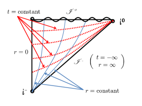
Figure 1: The Penrose diagram of the $D$-dimensional spacetime (9c) with $c_{0}=-1$ , $t\leq 0$ , $M=0$ , is depicted. The wavy line at $t=0$ is the spacelike singularity.

The Penrose diagram for the spacetime with $M=0$ is shown in Fig. 1. The angular coordinates on $S^{D-p-2}$ and also $p$-dimensional worldvolume coordinates have been suppressed. The spacetime is geodesically incomplete, since radial null geodesics reach singularities at a finite affine parameter value.

Although there is a curvature singularity at $t=0$ , the singularity in this solution is spacelike. One way to see this is to note that outgoing radial light rays satisfy (18), so that as $t\rightarrow 0$, $r$ approaches $r_{0}$ , as $1+\beta>0$ .

Finally we calculate the radial null geodesics numerically in a dynamical $p$-brane background with $M\neq 0$ and $c_{0}=-1$ . We show the motion of radial null geodesics for a 1-brane (Fig 2), 2-brane (Fig 3), 3-brane (Fig 4), and M5-brane (Fig 5), respectively. The left panels (a) in Figs. 2 - 5 show that past directed null geodesics reach the naked singularity in finite affine parameter. The ”nonsingular” initial data evolves into a timelike singularity. Since we can set a ”regular and smooth” initial data for the M5-brane, this leads to be a violation of cosmic censorship. On the other hand, we illustrate that past directed null geodesics can reach past null infinity in the right panels (b) in Figs. 2 - 5 .

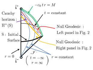
Figure 6: The Penrose diagram of the $D$-dimensional spacetime (9) with $M\neq 0$ , $c_{0}<0$ , $D-p-3=1$ is depicted in left panel. The right panel in this figure shows Penrose diagram for the solution (9) with $c_{0}<0$ , $D-p-3\geq 2$ . In both cases, the green line (double line) at $h=0$ is the timelike singularity. The dot-dash (purple) line shows the Cauchy horizon H⁺(S). In the domain $D^{+}$(S) which is inside of a Cauchy horizon H⁺(S), the null geodesics passing through the initial surface S evolves far into the past infinitely. We focus on the behavior of null geodesic near the double line. The naked singularity appears first at large $r$ as the time increases. The past directed null geodesics (red line or dotted line) corresponding to the left panel in Figs. 2, 3, 4, and 5 reach a singularity in finite affine parameter while another past directed null geodesics (orange line or bold line) corresponding to the right panel in Figs. 2, 3, 4, and 5 never hit the singularity. The difference between them comes from the initial data. We see that the asymptotic behavior of the null curves depends crucially on whether $r$ is inside or outside the Cauchy horizon. If the null curve is outside of the Cauchy horizon, the past directed radial null geodesics always reach the singularity. The dotted (red) line shows that the ”regular and smooth” initial data evolves into a timelike curvature singularity. For M-brane, we can set a perfectly smooth and regular initial data. Then, the null geodesics in the dynamical M-brane background hit a timelike curvature singularity at $h=0$ . This suggests a violation of cosmic censorship in the dynamical $p$-brane background.

The Penrose diagram for the entire spacetime with $M\neq 0$, is shown in Fig. 6. We depict two past directed null geodesics in Fig. 6. Although the red (dotted) curve hits the naked singularity in finite affine parameter, the orange (bold) line can avoid the singularity. One can note that there is a null hypersurface $r=r_{\rm h}(t)$ in the dynamical $p$-brane background. The null geodesics outside of it hit the timelike singularity while the past directed radial null geodesics inside of this hypersurface can reach past null infinity. There is a Cauchy horizon (dot-dash line) in the dynamical $p$-brane solution (9). In the domain $D^{+}$(S) which is inside of a Cauchy horizon H⁺(S), the null geodesics can pass through the initial surface S and evolves far into the past infinitely.

We will see that the $p$-brane background changes the causal structure of the dynamical solution without $p$-brane. When one adds a single $p$-brane, the spacelike singularity is replaced by a timelike one which is visible to observers in the spacetime. So this solution has a naked singularity. The naked singularity appears first at large $r$, and the null geodesic cannot be extended beyond $r=\left(-M/c_{0}\,t\right)^{1/D-p-3}$ .

The dynamical $p$-brane backgrounds in general have a curvature singularity at $r=0$ , if the dilaton is non-trivial. The near $p$-brane geometry is the same as the static one because $h(t,r)\rightarrow h_{1}(r)$ as $r\rightarrow 0$ . Then the geometry approaches the static solution. Although we expect that the singularity at $r=0$ can be resolved in string theory Johnson:1999qt ; Jarv:2000zv ; Peet:1999nh ; Johnson:2000ch ; Yamaguchi:2001yd , the timelike singularity at $h=0$ is still left. If the dynamical $p$-brane background has a horizon geometry, we can regard the present time-dependent solution as a black hole. In fact, we know that M-branes give black hole spacetimes in the static limit due to vanishing dilaton Maeda:2009zi . From the Eq. (8), the dynamical M-brane background becomes regular at $y^{i}=y^{i}_{l}$ because of the Ricci scalar for the M-brane being constant. Since the perfectly smooth and regular initial data in the far past evolves into a timelike curvature singularity at $h=0$, the cosmic censorship is violated in the M5-brane background.

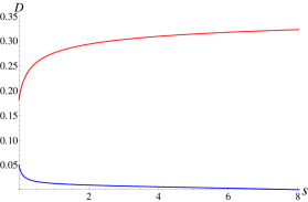
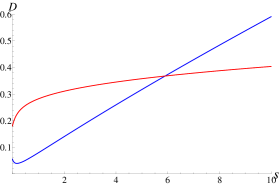
Figure 2: The radial null geodesic of 1-brane in the five-dimensional spacetime (9) is depicted. We have fixed $dt/ds|_{s=0}=-1$ , $c_{0}=-1$ , $M=1$ , in the solution (9). The red (dashed) and blue (solid) lines correspond to the radial null geodesic $r/10$ and function $h$, respectively. ”$D$” in the vertical axis indicates the value of $r/10$, or the function $h$, while ”$s$” in the horizontal axis denotes the affine parameter. If we set $r(s=0)=1.82$ and $t(s=0)=-c_{0}^{-1}M[r(s=0)]^{-1}$, the function $h$ settles down to zero in left panel. The past directed null geodesic hits the singularity. Then, the initially ”smooth and regular” data evolves into a timelike singularity. The right panel illustrates the case in which $r(s=0)$, $t(s=0)$ are given by $r(s=0)=1.8$, $t(s=0)=-c_{0}^{-1}M[r(s=0)]^{-1}$ , respectively. Since the null geodesic can extend to past null infinity, it never actually reaches the singularity.

Figure 3: We give the radial null geodesic of 2-brane in the six-dimensional spacetime (9). We have set $dt/ds|_{s=0}=-1$ , $c_{0}=-1$ , $M=1$ , in the solution (9). The red and blue curves show the behavior of radial null geodesic $r/10$ and function $h$, respectively. ”$D$” in the vertical axis indicates the value of $r/10$, or the function $h$, while ”$s$” in the horizontal axis denotes the affine parameter. The left panel illustrates the case in which the initial condition of $r$, $t$ are fixed by $r(s=0)=1.83$ , $t(s=0)=-c_{0}^{-1}M[r(s=0)]^{-1}$ , respectively. The geodesic hits a curvature singularity in finite affine parameter, and the spacetime is null geodesically incomplete. The ”regular and smooth” initial data becomes a timelike singularity as the time evolves. In the right panel, we set $r(s=0)=1.5$ , $t(s=0)=-c_{0}^{-1}M[r(s=0)]^{-1}$ . The null geodesic reaches past null infinity while it never hits the singularity.

Figure 4: We illustrate the motion of radial null geodesic for 3-brane in the seven-dimensional spacetime. In this plot, the parameters have been set to $dt/ds|_{s=0}=-1$ , $c_{0}=-1$ , $M=1$ , in the solution (9). We depict the dynamics of radial null geodesic $r/10$ (red line) and function $h$ (blue line), respectively. ”$D$” in the vertical axis indicates the value of $r/10$, or the function $h$, while ”$s$” in the horizontal axis denotes the affine parameter. The left panel shows that the function $h$ approaches zero for the present choice of parameters. Here the initial data $r(s=0)$ , $t(s=0)$ have been fixed by $r(s=0)=1.82$ , $t(s=0)=-c_{0}^{-1}M[r(s=0)]^{-1}$ , respectively. The ”nonsingular” initial conditions evolve into a naked singularity. A typical configuration for fixing $r(s=0)=1.5$ is also shown in right panel. The null geodesic never reaches the timelike singularity.

Figure 5: We illustrate the motion of radial null geodesic for M5-brane in the eleven-dimensional spacetime. The parameters have been set to $dt/ds|_{s=0}=-1$ , $c_{0}=-1$ , $M=1$ , in this plot. In the left panel, ”$D$” in the vertical axis indicates the value of $r/50$ for red line, or the function $h$ for blue line . In the left panel, ”$D$” in the vertical axis denotes the value of $r/10$ for red line, or the function $h$ for blue line. In both panels, ”$s$” in the horizontal axis shows the affine parameter. The left panel shows that the function $h$ goes to zero for the present choice of parameters. The parameters $r(s=0)$ and $t(s=0)$ have been set to $r(s=0)=1.88$ , $t(s=0)=-c_{0}^{-1}M[r(s=0)]^{-3}$ , respectively . One can note that the regular initial data evolves into a naked singularity. Then, this would allow one to find violations of cosmic censorship. On the other hand, we have set $r(s=0)=1.85$ , $t(s=0)=-c_{0}^{-1}M[r(s=0)]^{-3}$ , in right panel. In this case, the null geodesic never hits the timelike singularity.

III.2 The dynamical $p$-brane depending on the null coordinate

Here we discuss the radial null geodesics on the dynamical $p$-brane background whose metric are given by the null coordinates Binetruy:2007tu ; Maeda:2009tq :

$$ds^{2}=h^{a}(u,r)\left(-2du\,dv+\delta_{PQ}dx^{P}dx^{Q}\right)+h^{b}(u,r)\left(dr^{2}+r^{2}w_{mn}dz^{m}dz^{n}\right)\,,$$ (19a)

$$u=\frac{1}{\sqrt{2}}\left(t-x\right)\,,~{}~{}~{}~{}~{}~{}v=\frac{1}{\sqrt{2}}\left(t+x\right)\,,$$ (19b)

$$h(u,r)=h_{0}(u)+h_{1}(r),~{}~{}~{}~{}~{}h_{0}(u)=c_{0}u\,,~{}~{}~{}~{}~{}h_{1}(r)=\frac{M}{r^{D-p-3}}\,,$$ (19c)

where $\delta_{PQ}$ is the metric of $(p-1)$-dimensional Euclid space, and we assume $d_{\rm Y}=0$ . Since the geodesic is null, the geodesic equation yields

$$\dot{u}=fh^{-a}\,,~{}~{}~{}~{}\dot{v}=f^{-1}h^{b}\dot{r}^{2}\,,$$ (20a)

$$\ddot{r}=\frac{(a+b)(D-p-3)M}{2h}\frac{\dot{r}^{2}}{r^{D-p-2}}-b\,f\,c_{0}\,h^{-b}\,\dot{r}\,,$$ (20b)

where $f$ is constant. First we study the null geodesic without $p$-brane. The solution of geodesic equation with $M=0$ is given by

$$u(s) = \left[(1+a)\left(c_{0}^{-a}\,f\,s+u_{0}\right)\right]^{\frac{1}{1+a}},$$ (21a)

$$r(s) = r_{0}\ln\left|c_{0}^{-a}\,f\,s+u_{0}\right|+r_{1}\,,$$ (21b)

where $u_{0}$, $r_{0}$, $r_{1}$ are constants . If we set $r_{0}<0$ , the singularity in this background (19) is not spacelike but null, so that as $u\rightarrow 0$, $r\rightarrow\infty$ . Hence, observers do not lose causal contact as they approach the singularity. This is an important difference between the solution with $M=0$ , and standard FLRW universe with spacelike singularity.

Next we solve the radial null geodesic equation numerically in the dynamical $p$-brane background (19) in the case of $M\neq 0$ and $f\neq 0$ . The motion of radial null geodesics for 1-brane, 2-brane are shown in Figs. 7 and 8, respectively. The left panels (a) in Figs. 7 and 8 illustrate the past directed null geodesics reach the timelike singularity in finite affine parameter. We show that past directed null geodesics can reach past null infinity in the right panels (b) in Figs. 7 and 8. Although the evolution of the null geodesic depends on the initial data, the ”regular and smooth” initial data in the far past (19) evolves into a spacetime with a naked singularity.

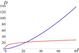
Figure 7: The radial null geodesic of 1-brane in the five-dimensional spacetime (19a) is depicted. We have fixed $dr/ds|_{s=0}=1$ , $c_{0}=-1$ , $f=-1/2$ , $M=1$ , in the solution (19). The red (dashed) and blue (solid) lines correspond to the radial null geodesic $r$ and function $h$, respectively. In the left panel, ”$D$” in the vertical axis indicates the value of $r$ for red line, or the function $10^{2}\,h$ for blue line . On the other hand, ”$D$” in the vertical axis gives the value of ${\rm e}^{r}$ for red line, or the function $h$ for blue line in the right panel. In both panels, ”$s$” in the horizontal axis denotes the affine parameter. If we set the initial value of radial coordinate and time $r(s=0)=1.95$ , $u(s=0)=-c_{0}^{-1}M[r(s=0)]^{-1}$ , a singularity appears at $s=0.104$ in left panel. The past directed null geodesic hits the timelike singularity. The ”smooth and regular” initial data evolves into a timelike singularity. The right panel shows the case in which $r(s=0)$ , $u(s=0)$ are given by $r(s=0)=1.7$ , $u(s=0)=-c_{0}^{-1}M[r(s=0)]^{-1}$ , respectively. The null geodesic can reach past null infinity.

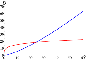
Figure 8: We give the radial null geodesic of 2-brane in the six-dimensional spacetime (19a). We have fixed $dr/ds|_{s=0}=1$ , $c_{0}=-1$ , $f=-1/2$ , $M=1$ , in the solution (19). The red (dashed) and blue (solid) lines correspond to the past directed radial null geodesic $r$ and function $h$, respectively. ”$D$” in the vertical axis shows the value of $r$ for red line, or the function $10^{2}\,h$ for blue line in the left panel. In the right panel, ”$D$” in the vertical axis indicates the value of ${\rm e}^{r}$ for red line, or the function $h$ for blue line. In both panels, ”$s$” in the horizontal axis denotes the affine parameter. The left panel shows the case in which the initial condition of $r$ , $u$ are fixed by $r(s=0)=1.99$ , $u(s=0)=-c_{0}^{-1}M[r(s=0)]^{-1}$ , respectively. Since the function $h$ eventually vanishes at $s=0.0176$ . the past directed radial null geodesic hits a timelike singularity. The ”regular and smooth” initial data evolves into a timelike curvature singularity. The right panel depicts the past directed radial null geodesic which does not reach the singularity. The initial value of $r$ , $u$ are fixed by $r(s=0)=1.70$ , $u(s=0)=-c_{0}^{-1}M[r(s=0)]^{-1}$ , respectively.

IV Discussions

In the present paper, we have discussed the causal structure and the behavior of the singularity in the dynamical $p$-brane background which can be viewed as a family of time dependent solutions to the Einstein-Maxwell-dilaton theory Horne:1993sy . This background gives an example to test cosmic censorship. The dynamical solution in this paper describes an arbitrary number of $p$-branes or extremal charged black holes in a expanding or contracting universe Maeda:2009zi . The spacetime collapses to a spacelike or null singularity without $p$-branes. However, the spacelike or null singularity turns into a naked one if we add a single $p$-brane. Hence, regular initial data in the far past evolves into a timelike curvature singularity even if there is only one $p$-brane. This implies that cosmic censorship fails for the dynamical $p$-brane background. These results are consistent with the analysis of Horne & Horowitz Horne:1993sy .

As we have said in section III, the dynamical $p$-brane backgrounds with non-trivial dilaton have singularities at $r=0$ and $h=0$ . In the $p$-brane solutions, the event horizon shrinks down to zero size in the extremal limit. Then there is singularity at $r=0$ in the $p$-brane backgrounds. These solutions describe an extremal black hole in the expanding or collapsing universe Maeda:2009zi ; Horne:1993sy . The singularities at $h=0$ in the solutions (9) and (19) are generated by the gravitational collapse. If we consider the $p$-brane solution which moves slightly away from the extremal limit, the spacelike surface $r=0$ will become a nonsingular horizon shielding a spacelike or null singularity inside. The slight change of the brane charge does not modify the solution asymptotically. Since the timelike singularity at large $r$ will be present, nonsingular initial data evolves into a naked singularity. This implies that cosmic censorship is violated in the non extremal $p$-brane background. However, in order to study whether cosmic censorship fails for this background, we have to construct the non-extremal dynamical $p$-brane solution.

If the background has the vanishing or trivial dilaton, there is dynamical brane solutions whose have event horizon at $r=0$ . Then, we can set smooth initial data evolving into a timelike curvature singularity. In this paper, we present that the cosmic censorship is violated for the dynamical M5-brane system in eleven-dimensional supergravity.

The cosmic censorship Penrose:1964wq ; Penrose:1969pc , which was supposed long times ago following the recognition of the special role of forming the singularity, is violated by the time-dependence of fields in the context of general relativity. However, in the region of the dynamical $p$-brane near the naked singularity, the curvature of the spacetime becomes very large. Then we have to indeed discuss this issue in the quantum theory of gravity, such as string theory. Moreover, the string loop correction will be important if observers approach the singularity on the basis of string theory. Hence, we can say very little at this time about the violation of the cosmic censorship in string theory unless higher order string $\alpha^{\prime}$ corrections in the solution is included.

Appendix

Appendix A Dynamical $p$-brane background

In this appendix, we work out the explicit form of the components of Einstein equations for a general metric which is compatible with the expected form of the sought for dynamical $p$-brane solutions.

For the $D$-dimensional action (1), the field equations are given by

$$R_{MN}=\frac{1}{2}\partial_{M}\phi\partial_{N}\phi$$

$$~{}~{}~{}~{}~{}~{}+\frac{1}{2}\frac{{\rm e}^{\epsilon c\phi}}{\left(p+2\right)!}\left[\left(p+2\right)F_{MA_{2}\cdots A_{\left(p+2\right)}}{F_{N}}^{A_{2}\cdots A_{\left(p+2\right)}}-\frac{p+1}{D-2}\,g_{MN}\,F^{2}_{\left(p+2\right)}\right],$$ (22a)

$${\triangle}\phi-\frac{1}{2}\frac{\epsilon c}{\left(p+2\right)!}{\rm e}^{\epsilon c\phi}F^{2}_{\left(p+2\right)}=0\,,$$ (22b)

$$d\left[{\rm e}^{\epsilon c\phi}\ast F_{\left(p+2\right)}\right]=0\,,$$ (22c)

where $R_{MN}$, ${\triangle}$ denote the Ricci tensor, Laplace operator with respect to the $D$-dimensional metric $g_{MN}$ , respectively and the constants $c$ , $\epsilon$ are defined by

$$c^{2} = N-\frac{2(p+1)(D-p-3)}{D-2},$$ (23a)

$$\epsilon = \left\{\begin{array}[]{cc}+&{\rm if~{}the}~{}p-{\rm brane~{}is~{}electric}\\ -&~{}~{}~{}{\rm if~{}the}~{}p-{\rm brane~{}is~{}magnetic}\,.\end{array}\right.$$ (23d)

Here $N$ is constant. We will consider general metrics with components depending on not only coordinates of transverse space to $p$-brane but also worldvolume ones. Hence, the time is not translational invariant. To begin with we do not impose any symmetry in $D$-dimensional spacetime. Then we consider a particular case in which we have indeed $(p+1)$-dimensional Minkowski spacetime and $(D-p-1)$-dimensional Euclidean space. The $D$-dimensional metric of dynamical $p$-brane is written in the general form

$$ds^{2}=h^{a}(x,y)q_{\mu\nu}({\rm X})dx^{\mu}dx^{\nu}+h^{b}(x,y)\gamma_{ij}({\rm Y})dy^{i}dy^{j}\,,$$ (24)

where $q_{\mu\nu}({\rm X})$ is the $(p+1)$-dimensional metric depending only on the $(p+1)$-dimensional coordinates $x^{\mu}$, $\gamma_{ij}({\rm Y})$ is the $(D-p-1)$-dimensional metric depending only on the $(D-p-1)$-dimensional coordinates $y^{i}$, and we assume that the parameters $a$, $b$ in the metric (4a) are given by

$$a=-\frac{4\left(D-p-3\right)}{N\left(D-2\right)},~{}~{}~{}~{}~{}~{}~{}~{}~{}b=\frac{4\left(p+1\right)}{N\left(D-2\right)}.$$ (25)

The dynamical $p$-brane solutions are characterized by function, $h$, depending on the $(D-p-1)$-dimensional coordinates $y^{i}$ transverse to the corresponding brane as well as the $(p+1)$-dimensional world-volume coordinate $x^{\mu}$ .

The expression for the field strength $F_{\left(p+2\right)}$, and scalar field $\phi$ is given by

$${\rm e}^{\phi} = h^{2\epsilon c/N}\,,$$ (26a)

$$F_{\left(p+2\right)} = \frac{2}{\sqrt{N}}\,d\left[h^{-1}(x,y)\right]\wedge\sqrt{-q}\,dx^{0}\,\wedge\,dx^{1}\wedge\,\cdots\,\wedge\,dx^{p}\,,$$ (26b)

where $q$ is the determinant of the metric $q_{\mu\nu}$ .

Let us first consider the gauge field Eq. (22c). Using the assumptions (24) and (26), we have

$$\partial_{\mu}\partial_{i}h=0\,,~{}~{}~{}~{}~{}~{}{\triangle}_{{\rm Y}}h=0\,,$$ (27)

where ${\triangle}_{{\rm Y}}$ is the Laplace operator constructed from the metric $\gamma_{ij}({\rm Y})$ .

From Eq. (27) , the function $h$ can be expressed as

$$h(x,y)=h_{0}(x)+h_{1}(y)\,,~{}~{}~{}~{}~{}~{}{\triangle}_{{\rm Y}}h_{1}=0\,.$$ (28)

Using the assumptions (24) and (26), the Einstein equations are reduced to

$$R_{\mu\nu}({\rm X})-\frac{4}{N}h^{-1}D_{\mu}D_{\nu}h_{0}+\frac{2}{N}\left(1-\frac{4}{N}\right)h^{-2}\partial_{\mu}h_{0}\partial_{\nu}h_{0}$$

$$~{}~{}~{}~{}-\frac{a}{2}h^{-2}q_{\mu\nu}\left[h{\triangle}_{{\rm X}}h_{0}-\left(1-\frac{4}{N}\right)q^{\rho\sigma}\partial_{\rho}h_{0}\partial_{\sigma}h_{0}\right]=0,$$ (29a)

$$R_{ij}({\rm Y})-\frac{b}{2}h^{-2+\frac{4}{N}}\gamma_{ij}\left[h{\triangle}_{{\rm X}}h_{0}-\left(1-\frac{4}{N}\right)q^{\rho\sigma}\partial_{\rho}h_{0}\partial_{\sigma}h_{0}\right]=0,$$ (29b)

where we have used (28).

Substituting ansatz for fields (26), metric (24), and the equation (28) into the equation of motion for scalar field (22b), we find

$$\frac{\epsilon c}{N}h^{-b-2+\frac{4}{N}}\left[h{\triangle}_{{\rm X}}h_{0}-\left(1-\frac{4}{N}\right)q^{\rho\sigma}\partial_{\rho}h_{0}\partial_{\sigma}h_{0}\right]=0.$$ (30)

Hence if we assume $c\neq 0$, and

$$R_{\mu\nu}({\rm X})=0\,,~{}~{}~{}~{}~{}R_{ij}({\rm Y})=0\,,~{}~{}~{}~{}~{}N=4\,,$$ (31a)

$$D_{\mu}D_{\nu}h_{0}=0\,,~{}~{}~{}~{}~{}{\triangle}_{{\rm Y}}h_{1}=0\,,$$ (31b)

the field equations are solved with the condition (28).

Let us consider the case in more detail

$$q_{\mu\nu}({\rm X})=\eta_{\mu\nu},~{}~{}~{}~{}~{}\gamma_{ij}({\rm Y})=\delta_{ij}\,,$$ (32)

where $\eta_{\mu\nu}$ is the $(p+1)$-dimensional Minkowski metric, $\delta_{ij}$ is $(D-p-1)$-dimensional Euclidean metrics, respectively. The solution for the functions $h_{0}$ and $h_{1}$ can be obtained explicitly as (6) Binetruy:2007tu ; Binetruy:2008ev ; Maeda:2009zi ; Uzawa:2010zza ; Minamitsuji:2010kb ; Minamitsuji:2010uz ; Uzawa:2014dra .

Now we introduce a new time coordinate $\tau$ by

$$\frac{\tau}{\tau_{0}}=\left(c_{0}t+\bar{c}\right)^{\frac{D+p-1}{2(D-2)}}\,,~{}~{}~{}~{}~{}\tau_{0}=\frac{2\left(D-2\right)}{c_{0}\left(D+p-1\right)}\,,$$ (33)

where we have assumed $c_{0}>0$, $c_{A}=0~{}(A=1,2,\cdots,p)$ for simplicity. Then, the $D$-dimensional metric (24) is given by

$$ds^{2} = \left[1+\left(\frac{\tau}{\tau_{0}}\right)^{-\frac{2(D-2)}{D+p-1}}h_{1}\right]^{-\frac{D-p-3}{D-2}}\left[-d\tau^{2}+\left(\frac{\tau}{\tau_{0}}\right)^{-\frac{2(D-p-3)}{D+p-1}}\delta_{AB}dx^{A}dx^{B}\right.$$ (34)

$$\left.+\left\{1+\left(\frac{\tau}{\tau_{0}}\right)^{-\frac{2(D-2)}{D+p-1}}h_{1}\right\}\left(\frac{\tau}{\tau_{0}}\right)^{\frac{2(p+1)}{D+p-1}}\gamma_{ij}dy^{i}dy^{j}\right],$$

where the metric $\delta_{AB}$ is the spatial part of the $p$-dimensional Minkowski metric $\eta_{\mu\nu}$. If we set $h_{1}=0$, the scale factor of the $p$-dimensional space is proportional to $\tau^{-\frac{D-p-3}{D+p-1}}$, while that for the remaining $(D-p-1)$-dimensional space is proportional to $\tau^{\frac{p+1}{D+p-1}}$. Thus, in the limit when the terms with $h_{1}$ are negligible, which is realized in the limit $\tau\to\infty$, we have a Kaluza-Klein-type dynamical solution Binetruy:2007tu ; Binetruy:2008ev ; Maeda:2009zi ; Uzawa:2010zza ; Minamitsuji:2010kb ; Minamitsuji:2010uz ; Uzawa:2014dra .

Before closing this section, we discuss the dynamical $p$-brane solution on the exceptional case of $c=0$ . For $c=0$, the scalar field becomes constant because of the ansatz (26), and the equation of motion for the scalar field (22b) is automatically satisfied. The Einstein equations thus reduce to

$$R_{\mu\nu}({\rm X})=0\,,~{}~{}~{}~{}~{}R_{ij}({\rm Y})=\frac{a}{2}(p+1)\,\Lambda\,\gamma_{ij}({\rm Y})\,,~{}~{}~{}~{}~{}N=4\,,$$ (35a)

$$D_{\mu}D_{\nu}h_{0}=\Lambda\,q_{\mu\nu}({\rm X})\,,~{}~{}~{}~{}~{}{\triangle}_{{\rm Y}}h_{1}=0\,,$$ (35b)

where $\Lambda$ is a constant. The transverse space to the $p$-brane is not Ricci flat, but the Einstein space if $\Lambda\neq 0$ , If $q_{\mu\nu}({\rm X})=\eta_{\mu\nu}$, the function $h_{0}$ is no longer linear but quadratic in the coordinates $x^{\mu}$ Binetruy:2007tu ; Binetruy:2008ev ; Maeda:2009zi ; Uzawa:2010zza :

$$h_{0}(x)=\frac{\Lambda}{2}x^{\mu}x_{\mu}+c_{\mu}x^{\mu}+\bar{c}\,,$$ (36)

where $c_{\mu}$ and $\bar{c}$ are constant parameters.

Appendix B Global structure of static $p$-branes

In this Appendix, we give the geometrical structure of a static $p$-brane. Let us discuss the geodesics for a static $p$-brane solution. In general, the metric of $D$-dimensional spacetime for a static $p$-brane is given by

$$ds^{2}=h^{a}(r)\eta_{\mu\nu}({\rm X})dx^{\mu}dx^{\nu}+h^{b}(r)\delta_{ij}({\rm Y})dy^{i}dy^{j}\,,$$ (37a)

$$\gamma_{ij}({\rm Y})dy^{i}dy^{j}=dr^{2}+r^{2}w_{mn}dz^{m}dz^{n}\,,$$ (37b)

$$h_{1}(r)=1+\frac{M}{r^{D-p-3}}\,,$$ (37c)

where $w_{mn}$ is the metric of the $(D-p-2)$-dimensional sphere. The behavior of the function $h$ is classified into three classes depending on the dimensions of the $p$-brane, which is given by

$$({\rm i})~{}p<D-3\,,~{}~{}~{}~{}({\rm ii})~{}p=D-3\,,~{}~{}~{}~{}({\rm iii})~{}p=D-2\,.$$ (38)

Here, the function $h$ for the $(D-2)$-brane is given by the linear function of $r$. Then, the $D$-dimensional spacetime is not asymptotically flat. In string theory, this type of solution is classified as a ”massive brane”. We will review it in Appendix C . For the $(D-3)$-brane, the harmonic function $h$ diverges both at infinity and near the $(D-3)$-branes. Since there is no regular spacetime region near the $(D-3)$-branes, such solutions are not physically relevant. In this Appendix, we will discuss below only in the case of $p<D-3$ .

The geodesic equation (11b) in the static $p$-brane becomes

$$\ddot{r}-\frac{\left(a+b\right)\left(D-p-3\right)}{2r}\,\dot{r}^{2}=0\,.$$ (39)

This equation can be solved, to get

$$r(s) = \alpha_{2}\left[(1-\alpha)s+\alpha_{1}\right]^{\frac{1}{1-\alpha}}\,,~{}~{}~{}~{}{\rm for}~{}~{}~{}\left(a+b\right)\left(D-p-3\right)\neq 2\,,$$ (40a)

$$r(s) = \alpha_{4}\,{\rm e}^{\alpha_{3}\,s}\hskip 96.73918pt{\rm for}~{}~{}~{}\left(a+b\right)\left(D-p-3\right)=2\,,$$ (40b)

where $\alpha_{i}~{}(i=1,\cdots,4)$ are constants, and $\alpha$ is defined by

$$\alpha=\frac{1}{2}\left(a+b\right)\left(D-p-3\right)\,.$$ (41)

The singularity is located at $r=0$. For $\alpha\neq 1$ , the spacetime described by (4a) is geodesically incomplete because a null geodesic reaches it in finite $s$. Although the null geodesics never reach null singularity in the case of $\alpha=1$ and $N=4$ , we have to set $D>11$ . Hence, there is no solution for $\alpha=1$ in string or supergravity theory.

For $c_{0}=0$ and $\alpha\neq 1$ in the limit $r\rightarrow 0$, the radial null geodesic equation (11b) gives

$$t(s)=\pm\,\frac{\left(D-p-3-2\alpha\right)\alpha_{2}^{\frac{D-p-5}{2(1-\alpha)}}M^{1/2}}{a(D-p-3)(D-p-5)}\,\left[\left(1-\alpha\right)s+\alpha_{1}\right]^{-\frac{D-p-5}{2(1-\alpha)}}+t_{0}\,,$$ (42)

for $D-p-3\neq 0$ , $D-p-5\neq 0$ , and

$$t(s)=t_{1}\,\ln\left[\left(1-\alpha\right)s+\alpha_{1}\right]+t_{0}\,,$$ (43)

for $D-p-5=0$ . Here, $\alpha_{1}$ is given in (16), $t_{0}$, $t_{1}$ are constants, and $\alpha$ is defined by (41). As $r\rightarrow 0$ in the $p$-brane ($p\leq D-5$) , $t\rightarrow\pm\infty$ . On the other hand, for $D-p-5<0$, $t$ becomes finite value in the limit $r\rightarrow 0$ . Then the static $p$-brane solution has a null singularity at $r=0$ for $D-p-5\geq 0$ , while there is a timelike singularity at $r=0$ in the case of $D-p-5<0$ .

The global structure of the $p$-brane spacetime (9) with $c_{0}=0$ is similar to the extreme Reissner-Nordström solution. This global structure is described by the Penrose diagram as shown in Fig. 9, in which the angular coordinates on ${\rm S}^{D-p-2}$ and also the $p$-dimensional world-volume coordinates have been suppressed.

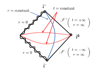
Figure 9: The Penrose diagram of the $D$-dimensional spacetime (9c) with $c_{0}=0$ , $N=4$ , $D-p-3=1$ is depicted in the left panel. The wavy line at $r=0$ is the timelike singularity. The right panel shows the Penrose diagram for the solution (9c) with $c_{0}=0$ , $N=4$ , $D-p-3\geq 2$ . The wavy lines at $r=0$ are the null singularities.

Appendix C Massive branes

In this appendix, we consider the case $D-p-3=-1$ and $d_{\rm Y}=0$ in the dynamical $p$-brane solution (7) , which corresponds to the massive brane in the case of $D=10$, $N=4$ Bergshoeff:1996ui ; Bergshoeff:1997ak . These solutions generally involve a function that is harmonic on the $(D-p-1)$-dimensional space transverse to the $(p+1)$-dimensional world-volume of the $p$-brane. For $D-p-3>0$, the transverse space has dimension three or greater. Thus, there exist harmonic functions that are constant at infinity. However, for $D-p-3<0$, the transverse space to $p$-brane has dimension two or less. Then, the asymptotic properties are therefore qualitatively different. Hence, we pay little attention so far to the case of $D-p-3<0$.

For $D-p-3=-1$ and $N=4$, the function of $h$ in the $D$-dimensional metric (4a) becomes

$$h(t,y)=h_{0}(t)+h_{1}(y)\,,~{}~{}~{}~{}h_{0}(t)=c_{0}\,t+\bar{c}\,,~{}~{}~{}~{}h_{1}(y)=1+\hat{c}\,y\,,$$ (44)

where $c_{0}$ , $\bar{c}$ , and $\hat{c}$ are constants .

We consider the Killing symmetry of the $p$-brane background with the case of $D-p-3=-1$. The solution for the Killing equation can be written by

$$\xi=\xi^{M}\frac{\partial}{\partial x^{M}}=k^{\mu}\frac{\partial}{\partial x^{\mu}}+l\,\frac{\partial}{\partial y}\,,$$ (45)

where $k^{\mu}$, $l$ are constant vectors. These vectors obey

$$k^{\mu}c_{\mu}+l\,\hat{c}=0\,.$$ (46)

We can also find another Killing vector field $\xi$ ,

$$\xi=\xi^{M}\frac{\partial}{\partial x^{M}}=l\,\frac{\partial}{\partial t}+k^{a}\,\frac{\partial}{\partial x^{a}}-c_{0}\,\frac{\partial}{\partial y}\,,$$ (47)

where the coordinate $x^{a}~{}(a=1,2,\cdots,p)$ denotes the spatial part of the $(p+1)$-dimensional Minkowski spacetime. Since the Killing vector has the norm

$$g_{MN}\xi^{M}\xi^{N}=h^{a}\left[-l^{2}+\delta_{ab}\,k^{a}k^{b}+hc_{0}^{2}\right],$$ (48)

the Killing vector is timelike in the case of $0<h<\left(l^{2}-\delta_{ab}\,k^{a}k^{b}\right)c_{0}^{-2}$ . If $h>\left(l^{2}-\delta_{ab}\,k^{a}k^{b}\right)c_{0}^{-2}$ , the Killing vector becomes spacelike. For $h=\left(l^{2}-\delta_{ab}\,k^{a}k^{b}\right)c_{0}^{-2}$ , it is null Chen:2005jp .

References

- (1) J. H. Horne and G. T. Horowitz, “Cosmic censorship and the dilaton,” Phys. Rev. D 48 (1993) R5457 [hep-th/9307177].
- (2) G. W. Gibbons, H. Lu and C. N. Pope, “Brane worlds in collision,” Phys. Rev. Lett. 94 (2005) 131602 [arXiv:hep-th/0501117].
- (3) W. Chen, Z. -W. Chong, G. W. Gibbons, H. Lu and C. N. Pope, “Horava-Witten stability: Eppur si muove,” Nucl. Phys. B 732 (2006) 118 [hep-th/0502077].
- (4) H. Kodama and K. Uzawa, “Moduli instability in warped compactifications of the type IIB supergravity,” JHEP 0507 (2005) 061 [arXiv:hep-th/0504193].
- (5) H. Kodama and K. Uzawa, “Comments on the four-dimensional effective theory for warped compactification,” JHEP 0603 (2006) 053 [arXiv:hep-th/0512104].
- (6) H. Kodama and K. Uzawa, “Moduli instability in warped compactification,” hep-th/0601100.
- (7) P. Binetruy, M. Sasaki and K. Uzawa, “Dynamical D4-D8 and D3-D7 branes in supergravity,” Phys. Rev. D 80 (2009) 026001 [arXiv:0712.3615 [hep-th]].
- (8) P. Binetruy, M. Sasaki and K. Uzawa, “Dynamical solution of supergravity,” arXiv:0801.3507 [hep-th].
- (9) K. i. Maeda, N. Ohta, M. Tanabe and R. Wakebe, “Supersymmetric Intersecting Branes in Time-dependent Backgrounds,” JHEP 0906 (2009) 036 [arXiv:0903.3298 [hep-th]].
- (10) K. i. Maeda, N. Ohta and K. Uzawa, “Dynamics of intersecting brane systems – Classification and their applications –,” JHEP 0906 (2009) 051 [arXiv:0903.5483 [hep-th]].
- (11) G. W. Gibbons and K. i. Maeda, “Black Holes in an Expanding Universe,” Phys. Rev. Lett. 104 (2010) 131101 [arXiv:0912.2809 [gr-qc]].
- (12) K. i. Maeda and M. Nozawa, “Black Hole in the Expanding Universe from Intersecting Branes,” Phys. Rev. D 81 (2010) 044017 [arXiv:0912.2811 [hep-th]].
- (13) K. Uzawa, “Dynamical intersecting brane solutions of supergravity,” AIP Conf. Proc. 1200 (2010) 541.
- (14) K. i. Maeda and M. Nozawa, “Black Hole in the Expanding Universe with Arbitrary Power-Law Expansion,” Phys. Rev. D 81 (2010) 124038 [arXiv:1003.2849 [gr-qc]].
- (15) M. Minamitsuji, N. Ohta and K. Uzawa, “Dynamical solutions in the 3-Form Field Background in the Nishino-Salam-Sezgin Model,” Phys. Rev. D 81 (2010) 126005 [arXiv:1003.5967 [hep-th]].
- (16) K. i. Maeda, M. Minamitsuji, N. Ohta and K. Uzawa, “Dynamical -branes with a cosmological constant,” Phys. Rev. D 82 (2010) 046007 [arXiv:1006.2306 [hep-th]].
- (17) M. Minamitsuji, N. Ohta and K. Uzawa, “Cosmological intersecting brane solutions,” Phys. Rev. D 82 (2010) 086002 [arXiv:1007.1762 [hep-th]].
- (18) K. Uzawa, “Cosmological intersecting brane solutions in string theory,” J. Phys. Conf. Ser. 259 (2010) 012032.
- (19) M. Nozawa and K. i. Maeda, “Cosmological rotating black holes in five-dimensional fake supergravity,” Phys. Rev. D 83 (2011) 024018 [arXiv:1009.3688 [hep-th]].
- (20) M. Minamitsuji and K. Uzawa, “Cosmology in -brane systems,” Phys. Rev. D 83 (2011) 086002 [arXiv:1011.2376 [hep-th]].
- (21) K. i. Maeda and M. Nozawa, “Black hole solutions in string theory,” Prog. Theor. Phys. Suppl. 189 (2011) 310 [arXiv:1104.1849 [hep-th]].
- (22) M. Minamitsuji and K. Uzawa, “Dynamics of partially localized brane systems,” Phys. Rev. D 84 (2011) 126006 [arXiv:1109.1415 [hep-th]].
- (23) K. -i. Maeda and K. Uzawa, “Dynamical brane with angles: Collision of the universes,” Phys. Rev. D 85 (2012) 086004 [arXiv:1201.3213 [hep-th]].
- (24) J. Blåbäck, B. Janssen, T. Van Riet and B. Vercnocke, “Fractional branes, warped compactifications and backreacted orientifold planes,” JHEP 1210 (2012) 139 [arXiv:1207.0814 [hep-th]].
- (25) M. Minamitsuji and K. Uzawa, “Cosmological brane systems in warped spacetime,” Phys. Rev. D 87 (2013) 046010 [arXiv:1207.4334 [hep-th]].
- (26) K. Uzawa and K. Yoshida, “Dynamical Lifshitz-type solutions and aging phenomena,” Phys. Rev. D 87 (2013) 106003 [arXiv:1302.5224 [hep-th]].
- (27) K. Uzawa and K. Yoshida, “Dynamical F-strings intersecting D2-branes in type IIA supergravity,” Phys. Rev. D 88 (2013) 066005 [arXiv:1307.3093].
- (28) J. Blåbäck, B. Janssen, T. Van Riet and B. Vercnocke, “BPS domain walls from backreacted orientifolds,” JHEP 1405 (2014) 040 [arXiv:1312.6125 [hep-th]].
- (29) K. Uzawa and K. Yoshida, “Probe brane dynamics on cosmological brane backgrounds,” Phys. Lett. B 738 (2014) 493 [arXiv:1401.3664 [hep-th]].
- (30) K. Uzawa, “Colliding -branes in the dynamical intersecting brane system,” Phys. Rev. D 90, 025024 (2014) [arXiv:1407.7406 [hep-th]].
- (31) D. Kastor and J. H. Traschen, “Cosmological multi - black hole solutions,” Phys. Rev. D 47 (1993) 5370 [arXiv:hep-th/9212035].
- (32) T. Maki and K. Shiraishi, “Multi - black hole solutions in cosmological Einstein-Maxwell dilaton theory,” Class. Quant. Grav. 10 (1993) 2171 [arXiv:1403.1320 [gr-qc]].
- (33) D. R. Brill, G. T. Horowitz, D. Kastor and J. H. Traschen, “Testing cosmic censorship with black hole collisions,” Phys. Rev. D 49 (1994) 840 [gr-qc/9307014].
- (34) R. Penrose, “Gravitational collapse and space-time singularities,” Phys. Rev. Lett. 14 (1965) 57.
- (35) R. Penrose, “Gravitational collapse: The role of general relativity,” Riv. Nuovo Cim. 1 (1969) 252 [Gen. Rel. Grav. 34 (2002) 1141].
- (36) T. Maki and K. Shiraishi, “Exact solutions for gravitational collapse with a dilaton field in arbitrary dimensions,” Class. Quant. Grav. 12 (1995) 159 [arXiv:1504.03062 [gr-qc]].
- (37) C. V. Johnson, A. W. Peet and J. Polchinski, “Gauge theory and the excision of repulson singularities,” Phys. Rev. D 61 (2000) 086001 [arXiv:hep-th/9911161].
- (38) L. Jarv and C. V. Johnson, “Orientifolds, M theory, and the ABCD’s of the enhancon,” Phys. Rev. D 62 (2000) 126010 [hep-th/0002244].
- (39) A. W. Peet, “Excision of ‘repulson’ singularities: A Space-time result and its gauge theory analog,” hep-th/0003251.
- (40) C. V. Johnson, “D-brane primer,” hep-th/0007170.
- (41) S. Yamaguchi, “Enhancon and resolution of singularity,” gr-qc/0108084.
- (42) E. Bergshoeff, M. de Roo, M. B. Green, G. Papadopoulos and P. K. Townsend, “Duality of type II 7 branes and 8 branes,” Nucl. Phys. B 470 (1996) 113 [hep-th/9601150].
- (43) E. Bergshoeff, Y. Lozano and T. Ortin, “Massive branes,” Nucl. Phys. B 518 (1998) 363 [hep-th/9712115].