Splitting methods for time integration of trajectories in combined electric and magnetic fields

Abstract

The equations of motion of a single particle subject to an arbitrary electric and a static magnetic field form a Poisson system. We present a second-order time integration method which preserves well the Poisson structure and compare it to commonly used algorithms, such as the Boris scheme. All the methods are represented in a general framework of splitting methods. We use the so-called $\phi$ functions, which give efficient ways for both analyzing and implementing the algorithms. Numerical experiments show an excellent long term stability for the new method considered.

I Introduction

The time integration of a particle motion due to electric and magnetic fields is a common task in several fields of science, from molecular dynamics to plasma physics and astrophysics. Various integration methods have been established within different scientific areas. A prominent example is the leap frog method, which is also called Boris pusher in the context of particle-in-cell (PIC) codes.

We consider here time-independent magnetic fields which, however, may be nonuniform in space. The electric field on the other hand is not subject to any constraints. A classical Coulomb system subject to a magnetic field serves as an example. If the particles within this system are moving sufficiently slow, the pairwise interaction can be described purely electrostatically and only the time invariant external magnetic field has to be taken into account.

In this article we review some second-order methods from the literature under a unifying framework: the methods are interpreted as splitting methods and the solutions of the subflows are given in terms of the so-called $\phi$ functions. This offers an economic way of stating, analyzing and implementing the methods. We also present a new second-order method based on the symmetric splitting of the Hamiltonian of the system. Further we discuss the structure preserving character of the methods regarding time symmetry, volume preservation and preservation of the system’s underlying Poisson structure.

The article is organized as follows. In Section II we formulate the equations of motion of a particle subject to an electric and a static magnetic field as a Poisson system, and we state some important properties of the exact flow of the system. In Section III we shortly discuss the corresponding properties we desire from the discrete flow given by the numerical integrator. In Section IV we give formulas for the maps corresponding to the subflows of different terms of the Poisson system and shortly discuss their structural properties. In Section V we present four time integrators, which are constructed using the formulas of Section IV and certain $\phi$ functions. In Section VI we give numerical results in which the integrators are compared on four different cases. The needed formulas for the matrix functions are given in the appendix (Section VIII).

II Equations of motion and their description as a Poisson system

The equations of motion for a particle with mass $m$ and charge $c$ subject to an electromagnetic field are given by the Lorentz force

$$m\ddot{q}=c(e+\dot{q}\times b),$$ (1)

where the electric field $e$ and the magnetic field $b$ are determined by a scalar potential $\Phi$ and a vector potential $A$, respectively, as

$$b =\nabla\times A,$$

$$e =-\nabla\Phi-\tfrac{\partial}{\partial t}A.$$

In the Lagrangian formalism the Lorentz force (1) can be derived from the Lagrangian

$$L=\tfrac{1}{2}m\|\dot{q}\|^{2}+c\,\dot{q}\cdot A-c\,\Phi,$$ (2)

which leads to the usual Hamiltonian formulation

$$H =\tfrac{1}{2m}\|p-c\,A\|^{2}+c\,\Phi,$$

$$p =m\dot{q}+c\,A.$$

However, we use a different formulation of the equations of motion, which exhibits both the Hamiltonian structure of the system and the splitting of the right-hand side into efficiently computable subflows. We use $p=m\dot{q}$ for the momentum and state the equations of motion as

$$\frac{{\rm d}}{{\rm d}t}q =\frac{p}{m},$$ (3)

$$\frac{{\rm d}}{{\rm d}t}p =F(q)+\Omega(q)p,$$

where $F(q)=c\,e(q)=-c\,\nabla\Phi(q)$ is the electric force and

$$\Omega(q)=\begin{bmatrix}0&\omega_{3}(q)&-\omega_{2}(q)\\ -\omega_{3}(q)&0&\omega_{1}(q)\\ \omega_{2}(q)&-\omega_{1}(q)&0\end{bmatrix}$$ (4)

corresponds to the cross product of the magnetic force as

$$\Omega(q)p=p\times\omega(q)=c\,\dot{q}\times b(q).$$

We use the matrix formulation of the cross product as it will simplify the analysis and derivation of the time integration methods.

The system (3) can be described as a Poisson system (HairerLubichWanner, , Ch. 7). Recall that a system of ordinary differential equations (ODEs) in $\mathbb{R}^{n}$ with a given initial value $y_{0}$ at $0$,

$$\frac{{\rm d}}{{\rm d}t}y=B(y)\nabla_{y}H(y),\quad y(0)=y_{0},$$ (5)

is called a Poisson system, if $B(y)$ is a skew-symmetric matrix which satisfies the identity

$$\sum\limits_{\ell=1}^{n} \Big{(}\frac{\partial B_{ij}(y)}{\partial y_{\ell}}B_{\ell k}(y)+\frac{\partial B_{jk}(y)}{\partial y_{\ell}}B_{\ell i}(y)$$ (6)

$$+\frac{\partial B_{ki}(y)}{\partial y_{\ell}}B_{\ell j}(y)\Big{)}=0\quad\textrm{ for }i,j,k=1,...,n.$$

In this case, $B(y)$ is also called a Poisson tensor. The exact flow $\varphi_{t}:\,\,y(0)\mapsto y(t)$ of any Poisson system is a Poisson map (also called noncanonically symplectic map), i.e., the Jacobian matrix of the flow satisfies

$$\left(\frac{\partial\varphi_{t}(y)}{\partial y}\right)B(y)\left(\frac{\partial\varphi_{t}(y)}{\partial y}\right)^{\sf T}=B\big{(}\varphi_{t}(y)\big{)}.$$ (7)

Moreover, it is time symmetric, i.e. $\varphi_{-h}=\varphi_{h}^{-1}$.

The ODE (3) can be written formally in the form (5) with the Hamiltonian

$$H(p,q)=\frac{1}{2m}\|p\|^{2}+c\,\Phi(q)$$ (8)

and the skew-symmetric structure matrix

$$B(y)=\begin{bmatrix}0&I\\ -I&m\Omega(q)\end{bmatrix}$$ (9)

by setting $y=\begin{bmatrix}q\\ p\end{bmatrix}$. We will denote from now on the conjugate variables as $y$ or $\begin{bmatrix}q\\ p\end{bmatrix}$, whichever is more convenient.

For the system matrix (9) we have the following. Let $b:\mathbb{R}^{3}\rightarrow\mathbb{R}^{3},\quad q\mapsto b(q)=\begin{bmatrix}b_{1}(q)&b_{2}(q)&b_{3}(q)\end{bmatrix}^{\sf T}$ be a differentiable function, and let the $3\times 3$ matrix (4) be defined by $\omega(q)=c\,m^{-1}b(q)$. Then a direct calculation using the relation (6) shows that $B(y)$ as in (9) defines a Poisson tensor if and only if $\,\,\nabla\cdot b(q)=0$. This is satisfied as Maxwell’s laws are assumed to hold for the magnetic field (e.g., we do not consider magnetic monopoles). Thus the ODE (3) can be written as a Poisson system (5).

The flow of a Hamiltonian system is volume preserving, i.e., it holds that

$$\det\,\frac{\partial\varphi_{t}(y)}{\partial y}=1.$$ (10)

The same is true for the exact flow of the system (5) with the structure matrix (9) as can be seen as follows. From the relation (7) it follows that

$$\left|\det\,\frac{\partial\varphi_{t}(y)}{\partial y}\right|=1,$$

as $\det\,B(y)=1$. Since $\det\,\frac{\partial\varphi_{t}(y)}{\partial y}$ is a continuous function of $t$, and since $\,\frac{\partial\varphi_{0}(y)}{\partial y}=I$, (10) holds also for the exact flow of the Poisson system.

As we consider only the motion of a single particle, the electrostatic force $F(q)$ will be time-independent. In case of many particles and pairwise forces this is not the case. However, the Poisson system (3) generalizes from dimension $6$ to $6N$ in a trivial way: $\Omega(q)$ is replaced by a $3N\times 3N$ block diagonal matrix consisting of $3\times 3$ blocks.

III Structure preserving integrators

It is desirable that the one-step map $\varphi_{h}:\,\,y_{0}\mapsto y_{1}$ given by the numerical flow satisfies the same structural properties as the exact flow of the ODE. The preservation of time symmetry or the Poisson structure implies good long time behavior for the numerical solution (see the backward error analysis of HairerLubichWanner ). The properties we want from the integrators are:

1. Time symmetry: $\varphi_{-h}=(\varphi_{h})^{-1}$.

2. The integrator gives a Poisson map, i.e., it holds that

   $$\left(\frac{\partial y_{1}}{\partial y_{0}}\right)B(y_{0})\left(\frac{\partial y_{1}}{\partial y_{0}}\right)^{\sf T}=B(y_{1}).$$ (11)

3. The preservation of volume:

   $$\det\,\frac{\partial y_{1}}{\partial y_{0}}=1.$$

Whether (11) is satisfied depends both on the integrator and the Poisson system considered. Moreover, the integrator has to respect the Casimirs (the first integrals of the Poisson system), which in general is difficult to verify for a nonlinear system matrix $B(y)$.

However, in some special cases one can show that these properties hold. That is the case for example if the integrator is a composition method resulting from a Hamiltonian splitting. This will be discussed in Section IV.

We will study analytically in Section V whether the considered integrators satisfy these properties.

IV Splitting methods

To have a common description for the various time integrators we state them in the framework of splitting methods and use the $\phi$ functions for representing the subflows containing the term $\Omega(q)p$. To this end, we write the Poisson system (3) as

$$\frac{{\rm d}}{{\rm d}t}y=\mathcal{T}(y)+\mathcal{E}(y)+\mathcal{B}(y),$$

where

$$\mathcal{T}\left(\begin{bmatrix}q\\ p\end{bmatrix}\right) =\begin{bmatrix}\frac{1}{m}p\\ 0\end{bmatrix},$$

$$\mathcal{E}\left(\begin{bmatrix}q\\ p\end{bmatrix}\right) =\begin{bmatrix}0\\ F(q)\end{bmatrix},$$

$$\mathcal{B}\left(\begin{bmatrix}q\\ p\end{bmatrix}\right) =\begin{bmatrix}0\\ \Omega(q)p\end{bmatrix}.$$

We denote the exact flows of the subsystems corresponding to $\mathcal{T}$, $\mathcal{B}$, $\mathcal{T}+\mathcal{B}$, etc. by $\varphi_{t}^{\mathcal{T}}$, $\varphi_{t}^{\mathcal{B}}$, $\varphi_{t}^{\mathcal{T}+\mathcal{B}}$, etc. This means that $\varphi_{t}^{\mathcal{T}}(y_{0})$ provides the exact solution of the system $w^{\prime}(t)=\mathcal{T}(w(t)),\,w(0)=y_{0}$ at time $t$, and so on. We further denote by $\varphi_{h}^{\mathcal{B}(y^{*})}$ the exact flow of the ODE with right-hand side $\mathcal{B}(y^{*})$, where $y^{*}=\begin{bmatrix}q^{*}\\ p\end{bmatrix}$. This means that the magnetic field is fixed at $q^{*}$, i.e. $\Omega(q)\equiv\Omega(q^{*})$. One easily verifies the following solutions for the exact flows:

$$\varphi_{h}^{\mathcal{T}}\left(\begin{bmatrix}q_{0}\\ p_{0}\end{bmatrix}\right) =\begin{bmatrix}q_{0}+\tfrac{h}{m}p_{0}\\ p_{0}\end{bmatrix},$$ (12)

$$\varphi_{h}^{\mathcal{E}}\left(\begin{bmatrix}q_{0}\\ p_{0}\end{bmatrix}\right) =\begin{bmatrix}q_{0}\\ p_{0}+hF(q_{0})\end{bmatrix},$$

$$\varphi_{h}^{\mathcal{B}(y^{*})}\left(\begin{bmatrix}q_{0}\\ p_{0}\end{bmatrix}\right) =\begin{bmatrix}q_{0}\\ \exp\big{(}h\Omega(q^{*})\big{)}p_{0}\end{bmatrix}.$$

We note that the so-called Rodrigues formula allows an efficient implementation of the matrix exponential $\exp(h\Omega)$ and the $\phi$ functions (see (38) and (43) of the Appendix).

We will also need the solutions of the subsystems corresponding to the fields $\mathcal{T}+\mathcal{B}(y^{*})$ and $\mathcal{E}+\mathcal{B}(q^{*})$. The flow corresponding to $\mathcal{T}+\mathcal{B}(y^{*})$ is given by the exact solution of the ODE

$$\frac{{\rm d}}{{\rm d}t}\begin{bmatrix}q\\ p\end{bmatrix}=\begin{bmatrix}0&\tfrac{1}{m}I\\ 0&\Omega(q^{*})\end{bmatrix}\begin{bmatrix}q\\ p\end{bmatrix},\quad$$

which can be expressed by the matrix exponential as

$$\begin{bmatrix}q(h)\\ p(h)\end{bmatrix}=\exp\left(\begin{bmatrix}0&\tfrac{1}{m}I\\ 0&\Omega(q^{*})\end{bmatrix}\right)\begin{bmatrix}q_{0}\\ p_{0}\end{bmatrix}.$$

Using (42) we see that

$$\varphi_{h}^{\mathcal{T}+\mathcal{B}(y^{*})}\left(\begin{bmatrix}q_{0}\\ p_{0}\end{bmatrix}\right)=\begin{bmatrix}q_{0}+\frac{h}{m}\phi_{1}\big{(}h\Omega(q^{*})\big{)}p_{0}\\ \exp(h\Omega(q^{*}))p_{0}\end{bmatrix},$$ (13)

where $\phi_{1}(z)=(\exp(z)-1)/z$.

On the other hand, the flow corresponding to the field $\mathcal{E}+\mathcal{B}$ is given by the exact solution of the ODE

$$\frac{{\rm d}}{{\rm d}t}\begin{bmatrix}q\\ p\end{bmatrix}=\begin{bmatrix}0\\ \Omega(q)p+F(q)\end{bmatrix}.$$

This solution is given by the variation-of-constants formula (44) as

$$\varphi_{h}^{\mathcal{E}+\mathcal{B}}\left(\begin{bmatrix}q_{0}\\ p_{0}\end{bmatrix}\right)=\begin{bmatrix}q_{0}\\ \exp\big{(}h\Omega(q_{0})\big{)}p_{0}+h\phi_{1}\big{(}h\Omega(q_{0})\big{)}F(q_{0})\end{bmatrix}.$$ (14)

We also state the solution for the flow corresponding to $\mathcal{T}+\mathcal{E}+\mathcal{B}$ in the particular case when both $F$ and $\Omega$ are constant. This is presented also in Chin using another formulation. The ODE corresponding to the flow is now

$$\frac{{\rm d}}{{\rm d}t}\begin{bmatrix}q\\ p\end{bmatrix}=\begin{bmatrix}0&\tfrac{1}{m}I\\ 0&\Omega\end{bmatrix}\begin{bmatrix}q\\ p\end{bmatrix}+\begin{bmatrix}0\\ F\end{bmatrix},$$

and its solution is given again by the variation-of-constants formula and by formula (42) as

$$\varphi_{h}\left(\begin{bmatrix}q_{0}\\ p_{0}\end{bmatrix}\right) =\exp\left(h\begin{bmatrix}0&\tfrac{1}{m}I\\ 0&\Omega\end{bmatrix}\right)\begin{bmatrix}q_{0}\\ p_{0}\end{bmatrix}$$

$$\qquad+h\phi_{1}\left(h\begin{bmatrix}0&\tfrac{1}{m}I\\ 0&\Omega\end{bmatrix}\right)\begin{bmatrix}0\\ F\end{bmatrix}$$

$$=\begin{bmatrix}q_{0}+\frac{h}{m}\phi_{1}(h\Omega)p_{0}+\frac{h^{2}}{m}\phi_{2}(h\Omega)F\\ \exp(h\Omega)p_{0}+h\phi_{1}(h\Omega)F\end{bmatrix},$$

where $\phi_{2}(z)=(\phi_{1}(z)-1)/z$.

We note that all of these substeps are time symmetric, i.e., $\varphi_{-h}^{\mathcal{T}}=(\varphi_{h}^{\mathcal{T}})^{-1}$, and so on.

We also note that the subflows (12) and (14) are volume preserving. Both the maps $\varphi_{h}^{\mathcal{E}+\mathcal{B}}:\,\,y_{0}\mapsto y_{1}$ and $\varphi_{h}^{\mathcal{B}(y^{*})}:\,\,y_{0}\mapsto y_{1}$ have the Jacobian

$$\frac{\partial y_{1}}{\partial y_{0}}=\begin{bmatrix}I&0\\ \frac{\partial p_{1}}{\partial q_{0}}&\exp\big{(}h\Omega(\widetilde{q})\big{)}\end{bmatrix},$$

where $\widetilde{q}=q_{0}$ for $\varphi_{h}^{\mathcal{E}+\mathcal{B}}$ and $\widetilde{q}=q^{*}$ for $\varphi_{h}^{\mathcal{B}(y^{*})}$. Its determinant is given by

$$\det\,\frac{\partial y_{1}}{\partial y_{0}}=\det\,\exp\big{(}h\Omega(\widetilde{q})\big{)}.$$

As the Cayley transform of a skew-symmetric matrix is a unitary matrix, and as $\det\,\exp(h\Omega(\widetilde{q}))$ is a continuous function of $h$ and $\exp(0)=I$, we find for the maps $\varphi_{h}^{\mathcal{E}+\mathcal{B}}$ and $\varphi_{h}^{\mathcal{B}(y^{*})}$ the relation

$$\det\,\frac{\partial y_{1}}{\partial y_{0}}=1.$$

Therefore both are volume preserving. One easily verifies from (12) that $\varphi^{\mathcal{T}}$ and $\varphi_{h}^{\mathcal{E}}$ are also volume preserving.

Splitting the Hamiltonian (8) gives subsystems corresponding to the right-hand sides

$$B(y)\,\nabla_{y}\tfrac{\|p\|^{2}}{2m}=\mathcal{T}(y)+\mathcal{B}(y)$$ (15)

and

$$B(y)\,\nabla_{y}\,c\Phi(q)=\mathcal{E}(y).$$ (16)

Both of these constitute Poisson systems of the form (5) with the system matrix (9) and with Hamiltonians $\tfrac{\|p\|^{2}}{2m}$ and $c\Phi(q)$, respectively. Therefore, the subflows $\varphi_{h}^{\mathcal{T}+\mathcal{B}}$ and $\varphi_{h}^{\mathcal{E}}$ are Poisson maps, as well as their compositions $\varphi_{h}^{\mathcal{E}}\circ\varphi_{h}^{\mathcal{T}+\mathcal{B}}$, etc.

V Methods

We will next state four time integration methods. They are formulated using the $\phi$ functions and the solutions of the subflows given in Section IV. Three of them can be found in the literature: the Boris–Buneman scheme BirdsallLangdon , the method of Chin Chin and the method of Spreiter and Walter SpreiterWalter . We also state a new method which is nearly symmetric and nearly preserves the Poisson structure (method C below).

V.1 Boris–Buneman scheme

The so-called Boris pusher BirdsallLangdon is undoubtedly the most common particle trajectory integrator used for PIC codes. It is a second-order accurate centered difference leap frog scheme, given by

$$\frac{q(t+\tfrac{h}{2})-q(t-\tfrac{h}{2})}{h} =\frac{p(t)}{m},$$

$$\frac{p(t+h)-p(t)}{h} =F\big{(}q(t+\tfrac{h}{2})\big{)}$$ (17)

$$+\Omega\big{(}q(t+\tfrac{h}{2})\big{)}\left(\frac{p(t+h)+p(t)}{2}\right).$$

PIC codes usually define the position with an offset of half a time step $h$ relative to the momentum. In (17) $q$ is updated alternatingly with $p$.

To formulate this scheme as a one-step method, we denote $q_{0}=\big{(}q(t+\tfrac{h}{2})+q(t-\tfrac{h}{2})\big{)}/2$, $q_{1/2}=q(t+\tfrac{h}{2})$, $p_{0}=p(t)$ and so on. Using this notation the linear drift operation corresponding to $\mathcal{T}$ can be split as

$$q_{1/2} =q_{0}+\tfrac{h}{2m}p_{0},$$ (18)

$$q_{1} =q_{1/2}+\tfrac{h}{2m}p_{1}.$$

The momentum change in between these drift operations is defined by the second equation of (17). Solving it for $p_{1}$ gives

$$p_{1}=h(I-\tfrac{h}{2}\hat{\Omega})^{-1}F(q_{1/2})+R(\tfrac{h}{2}\hat{\Omega})p_{0},$$

where $R(z)$ is the Cayley transform

$$R(z)=(1+z)(1-z)^{-1},$$

and $\hat{\Omega}=\Omega(q_{1/2})$. We note that both the resolvent $(I-\tfrac{h}{2}\hat{\Omega})^{-1}$ and $R(\tfrac{h}{2}\hat{\Omega})$ can be evaluated efficiently (see (45) and (46) of the Appendix). Since $R(z)+1=2(1-z)^{-1}$, we may rewrite the momentum step also as

$$p_{1}=\tfrac{h}{2}\big{(}R(\tfrac{h}{2}\hat{\Omega})+I\big{)}F(q_{1/2})+R(\tfrac{h}{2}\hat{\Omega})p_{0}.$$

From this one can easily read off that the mid-step can be split as

$$p^{+} =p_{0}+\tfrac{h}{2}F(q_{1/2}),$$ (19)

$$p^{++} =R(\tfrac{h}{2}\hat{\Omega})p^{+},$$

$$p_{1} =p^{++}+\tfrac{h}{2}F(q_{1/2}).$$

The steps (18) and (19) give together the approximation

$$\varphi_{h}\approx\varphi_{\frac{h}{2}}^{\mathcal{T}}\circ\varphi_{\frac{h}{2}}^{\mathcal{E}}\circ\widehat{\varphi}_{h}^{\mathcal{B}(y_{1/2})}\circ\varphi_{\frac{h}{2}}^{\mathcal{E}}\circ\varphi_{\frac{h}{2}}^{\mathcal{T}},$$ (20)

where $y_{1/2}=\varphi_{\frac{h}{2}}^{\mathcal{E}}\circ\varphi_{\frac{h}{2}}^{\mathcal{T}}(y_{0})$, and $\widehat{\varphi}_{h}^{\mathcal{B}(y_{1/2})}$ is given by

$$\widehat{\varphi}_{h}^{\mathcal{B}(y_{1/2})}\left(\begin{bmatrix}q\\ p\end{bmatrix}\right)=\begin{bmatrix}q\\ R\big{(}\tfrac{h}{2}\Omega(q_{1/2})\big{)}p\end{bmatrix}.$$

Since $R(-z)=R(z)^{-1}$, we have $\widehat{\varphi}_{-h}^{\mathcal{B}(y_{1/2})}=\left(\widehat{\varphi}_{h}^{\mathcal{B}(y_{1/2})}\right)^{-1}$. Therefore, (20) gives a symmetric method. We note that (20) is equivalent to the formulation (17) with the initial value $\varphi_{h/2}^{\mathcal{T}}(y_{0})$.

Since the Cayley transform of a skew-symmetric matrix is a unitary matrix, the subflow $\widehat{\varphi}_{h}^{\mathcal{B}(y_{1/2})}$ is also a volume preserving map (see the analysis of Section IV). And as also the maps $\varphi_{\frac{h}{2}}^{\mathcal{T}}$ and $\varphi_{\frac{h}{2}}^{\mathcal{E}}$ are volume preserving, the method (20) is volume preserving as a composition of volume preserving maps. The volume preservation property of the Boris scheme was also shown in Qinetal .

Replacing the Cayley transform by the exponential function in the mid-step, i.e., considering the splitting

$$\varphi_{h}\approx\varphi_{\frac{h}{2}}^{\mathcal{T}}\circ\varphi_{\frac{h}{2}}^{\mathcal{E}}\circ\varphi_{h}^{\mathcal{B}(y_{1/2})}\circ\varphi_{\frac{h}{2}}^{\mathcal{E}}\circ\varphi_{\frac{h}{2}}^{\mathcal{T}}$$ (21)

gives also a symmetric and volume preserving method. Both the Cayley transform and the matrix exponential rotate the momentum around the vector $b(q)$ in the mid-step. This can be seen as follows. Since $b(q)^{\sf T}\Omega(q)p_{0}=\tfrac{c}{m}b(q)^{\sf T}\big{(}p_{0}\times b(q)\big{)}=0$, we may deduce from the power series representations that

$$b(q)^{\sf T}\exp\big{(}h\Omega(q)\big{)}p_{0}=b(q)^{\sf T}R\big{(}\tfrac{h}{2}\Omega(q)\big{)}p_{0}=b(q)^{\sf T}p_{0}.$$ (22)

On the other hand, since $\Omega(q)$ is skew-symmetric both $\exp\big{(}h\Omega\big{)}$ and $R\big{(}\tfrac{h}{2}\Omega(q)\big{)}$ are unitary matrices, so that

$$\|\exp\big{(}h\Omega(q)\big{)}p_{0}\|_{2}=\|R\big{(}\tfrac{h}{2}\Omega(q)\big{)}p_{0}\|_{2}=\|p_{0}\|_{2}.$$ (23)

From (22) and (23) it follows that both give rotations around $b(q)$.

V.2 Chin’s schemes

Using the Lie operator formalism HairerLubichWanner , the following splitting methods are derived in Chin :

• Chin-a:

  $$\varphi_{h}^{a}(y_{0})=\varphi_{\frac{h}{2}}^{\mathcal{E}+\mathcal{B}}\circ\varphi_{h}^{\mathcal{T}}\circ\varphi_{\frac{h}{2}}^{\mathcal{E}+\mathcal{B}}(y_{0}),$$ (24)

• Chin-b:

  $$\varphi_{h}^{b}(y_{0})=\varphi_{\frac{h}{2}}^{\mathcal{T}}\circ\varphi_{h}^{\mathcal{E}+\mathcal{B}}\circ\varphi_{\frac{h}{2}}^{\mathcal{T}}(y_{0}).$$ (25)

Since the substeps are symmetric maps, both (24) and (25) give symmetric methods. Moreover, as the methods (24) and (25) are compositions of volume preserving maps (see Section IV), both of them are volume preserving as well.

We note that the methods of Chin become exactly energy preserving when $F=0$ Chin .

V.3 Symmetric splitting of the Hamiltonian

As a new method, we propose a symmetric splitting of the Hamiltonian for the Poisson system (5). This means that the right-hand side of the (5) is split into the flows (15) and (16) according to the Hamiltonian (8). Then, Strang splitting is applied to this decomposition giving the symmetric one-step method

$$y_{1}=\varphi_{\frac{h}{2}}^{\mathcal{E}}\circ\varphi_{h}^{\mathcal{T}+\mathcal{B}}\circ\varphi_{\frac{h}{2}}^{\mathcal{E}}(y_{0}).$$ (26)

For a constant magnetic field $\Omega(q)\equiv\Omega$ this splitting approach can be found in LeimkuhlerReich where it goes by the name of Scovel’s method; see also PatacchiniHutchinson .

The mid-step of (26), i.e., the solution

$$v_{1}=\varphi_{h}^{\mathcal{T}+\mathcal{B}}(v_{0}),\quad\textrm{where}\quad v_{0}=\varphi_{h/2}^{\mathcal{E}}(y_{0}),$$ (27)

can be computed efficiently using the formula (13) if the magnetic field is uniform. If the magnetic field is position dependent, some approximations have to be made.

We infer from (26) that the last substep $\varphi_{h/2}^{\mathcal{E}}$ changes only $p$. As the magnetic field depends only on $q$, we see from (13) that by using a symmetric approximation for (27), we get a symmetric approximation for (26).

The approaches we consider for the mid-step are the following ones:

1. The symmetric method

   $$w_{1}=\varphi_{\frac{h}{2}}^{\mathcal{T}+\mathcal{B}(w_{1})}\circ\varphi_{\frac{h}{2}}^{\mathcal{T}+\mathcal{B}(w_{0})}(w_{0})$$ (28)

   combined with fixed-point iteration. This approach can be found in EinkemmerOstermann .

2. The symmetric method

   $$w_{1}=\varphi_{h}^{\mathcal{T}+\mathcal{B}((w_{1}+w_{0})/2)}(w_{0})$$ (29)

   combined with fixed-point iteration.

3. Perform a symmetric high-order composition of either (28) or (29). For a description of composition schemes we refer to HairerLubichWanner . In numerical experiments we use the 8th-order scheme from SuzukiUmeno .

In the methods above the numerical strategy is to perform a fixed-point iteration for the implicit mid-step. This approach is also taken in EinkemmerOstermann . For the approach (28) this means that after the initial value

$$w_{1}^{(0)}=\varphi_{\frac{h}{2}}^{\mathcal{T}+\mathcal{B}(w_{0})}(w_{0}),\quad w_{0}=\varphi_{\frac{h}{2}}^{\mathcal{E}}(y_{0})$$

is computed, the iteration goes on as

$$w_{1}^{(k)}=\varphi_{\frac{h}{2}}^{\mathcal{T}+\mathcal{B}(w_{1}^{(k-1)})}(w_{1}^{(0)}).$$

Here $\varphi_{\frac{h}{2}}^{\mathcal{T}+\mathcal{B}(w_{1}^{(k-1)})}(w_{1}^{(0)})$ can be computed explicitly using the formula (13).

The implementation for (29) goes analogously. After the initial value

$$w_{1}^{(0)}=\varphi_{\frac{h}{2}}^{\mathcal{E}}(y_{0})$$

is computed, the iteration goes on as

$$w_{1}^{(k)}=\varphi_{\frac{h}{2}}^{\mathcal{T}+\mathcal{B}((w_{1}^{(k-1)}+w_{1}^{(0)})/2)}(w_{1}^{(0)}).$$

As shown in EinkemmerOstermann the method (26) with the approach (28) will be symmetric up to an order that equals the number of fixed-point iterations. It is easy to verify that the same holds true for (29). By the results of EinkemmerOstermann the same holds true for the third approach.

It is easily verified that the high-order composition scheme will also be a Poisson integrator up to an order of the scheme used for the mid-step (i.e., the relation (11) will be satisfied up to this order). Although the number of magnetic field evaluations increases considerably, the term $F(q)$ is still evaluated only once per time step, which may be beneficial in situations where the calculation of the electric field is more expensive than that of the magnetic field.

Since the flows of the subsystems resulting from a Hamiltonian splitting are Poisson maps, so is the composition (26); see also (HairerLubichWanner, , Ch. 7). As the method (26) is symmetric and a Poisson integrator, it has a modified Hamiltonian (see the backward error analysis of HairerLubichWanner ) and preserves the first integrals for exponentially long times.

The strategies 1-3 above give symmetric (or Poisson) maps up to a high order and we expect a good preservation of first integrals numerically.

V.4 The method of Spreiter and Walter

In SpreiterWalter a second-order accurate scheme is proposed which incorporates a homogeneous magnetic field in $z$-direction, and which overcomes the stability condition $h\omega_{c}\ll 2\pi$, where $\omega_{c}$ is the cyclotron frequency. We repeat here the derivation of this method using the $\phi$ functions which shortens the derivation considerably. As this derivation shows, the method can be seen as an exponential version of the velocity Verlet scheme. Integrating the Lorentz force law

$$\dot{p}(t)=\Omega p(t)+F(q(t))$$

with respect to $t$ gives an ODE for $q$,

$$\dot{q}(t)-\dot{q}(0)=\Omega\big{(}q(t)-q(0)\big{)}+\tfrac{1}{m}\int\limits_{0}^{t}F(q(s))\,{\rm d}s.$$ (30)

Under the assumption that $\tfrac{{\rm d}}{{\rm d}t}F(q(t))=\mathcal{O}(1)$, we can approximate the ODE (30) up to second order as

$$\dot{q}(t)=\Omega q(t)+\big{(}\dot{q}(0)-\Omega q(0)\big{)}+\frac{t}{m}F(q(0))+\mathcal{O}(t^{2}).$$

By the variation-of-constants formula (44) the solution for this ODE at $t=h$ is given by

$$q(h) =\exp(h\Omega)q(0)+h\phi_{1}(h\Omega)\big{(}\dot{q}(0)-\Omega q(0)\big{)}$$

$$\quad\quad+\tfrac{h^{2}}{m}\phi_{2}(h\Omega)F(q(0))+\mathcal{O}(h^{3})$$ (31)

$$=q(0)+\tfrac{h}{m}\phi_{1}(h\Omega)p(0)+\tfrac{h^{2}}{m}\phi_{2}(h\Omega)F(q(0))+\mathcal{O}(h^{3}).$$

This gives the time stepping formula for $q$. Integrating the Lorentz force law and using the variation-of-constants formula (44) once more yields

$$p(h)=\exp(h\Omega)p(0)+\int\limits_{0}^{h}\exp\big{(}(h-s)\Omega\big{)}F(q(s))\,{\rm d}s.$$

Using the fact that

$$F(q(s))=F(q(0))+s\dot{F}(q(0))+\mathcal{O}(s^{2})$$

and

$$\dot{F}(q(0))=\tfrac{1}{h}\big{(}F(q(h))-F(q(0))\big{)}+\mathcal{O}(h^{2})$$

we find that

$$p(h)= \exp(h\Omega)p(0)+h\phi_{1}(h\Omega)F(q(0))$$ (32)

$$+h\phi_{2}(h\Omega)\big{(}F(q(h))-F(q(0))\big{)}+\mathcal{O}(h^{3}).$$

The approximations (31) and (32) give together the one-step formula of Spreiter and Walter:

$$q_{1} =q_{0}+\tfrac{h}{m}\phi_{1}(h\Omega)p_{0}+\tfrac{h^{2}}{m}\phi_{2}(h\Omega)F(q_{0}),$$

$$p_{1} =\exp(h\Omega)p_{0}+h\phi_{1}(h\Omega)F(q_{0})$$

$$\quad+h\phi_{2}(h\Omega)\big{(}F(q_{1})-F(q_{0})\big{)}.$$

Since $\exp(h\Omega)\rightarrow 0$, $\phi_{1}(h\Omega)\rightarrow 1$ and $\phi_{2}(h\Omega)\rightarrow\tfrac{1}{2}$ as $\Omega\rightarrow 0$, we see that in the limiting case $\Omega\rightarrow 0$ the velocity Verlet scheme is obtained. We note that the method of Spreiter and Walter can be interpreted also as an exponential Taylor method KoskelaOstermann .

Despite of its similarity with the velocity Verlet scheme, we have not found any structure preserving properties for the method of Spreiter and Walter.

VI Numerical comparison of the integrators

In the first experiment, we compare the integrators for a particle motion in an inhomogeneous magnetic field in the absence of an electric field. Then, results for experiments including combined electric and magnetic fields are provided. The motion of a charged particle in a Penning trap Kretzschmar provides a suitable numerical test in the case of combined fields. In this setting the particle trajectory is a periodic orbit, formed by a superposition of three harmonic oscillators. In addition to the ideal Penning trap with a uniform magnetic field we consider two variations of this setup with static but nonuniform magnetic fields.

VI.1 2d particle motion in an inhomogeneous magnetic field

In the first experiment we consider an example provided in Chin : a particle of charge $c=-1$ and mass $m=1$ at initial position $q_{0}=\begin{bmatrix}1&0&0\end{bmatrix}^{{\sf T}}$ with initial velocity $v_{0}=\begin{bmatrix}0&v&0\end{bmatrix}^{{\sf T}}$ moves in a magnetic field $b=\begin{bmatrix}0&0&b_{z}\end{bmatrix}^{{\sf T}}$, $b_{z}=\frac{1}{q_{x}^{2}}$. The particle motion is composed of a periodic motion in the $xy$-plane and a $\nabla B$ drift in $y$-direction with drift velocity $v_{d}=\frac{v^{2}}{1+v}$. The drift reduced trajectory $\tilde{q}(t)=q(t)-\tilde{q}_{0}(t)$ forms an ellipse centered at $\tilde{q}_{0}(t)=\begin{bmatrix}x_{mid}&v_{d}\,t&0\end{bmatrix}^{{\sf T}}$ with $x_{mid}=\frac{1+v}{1+2v}$. $\tilde{q}(t)=\begin{bmatrix}\tilde{x}(t)&\tilde{y}(t)&0\end{bmatrix}^{{\sf T}}$ is given by

$$\tilde{x}(t) =\frac{v}{1+2v}\,\cos\rho(t),$$

$$\tilde{y}(t) =\frac{v}{(1+v)+\sqrt{1+2v}}\,\sin\rho(t).$$

One full orbit has the period $P=\frac{2\pi(1+v)}{(1+2v)^{\frac{3}{2}}}$.

The scalar potential is set $\Phi=0$ and the vector potential $A=\begin{bmatrix}0&A_{x}&0\end{bmatrix}^{{\sf T}}$ with $A_{x}=-\frac{1}{q_{x}}$. The Lagrangian takes the form $L=\tfrac{1}{2}\|\dot{q}\|^{2}+\,\dot{q}_{y}\tfrac{1}{q_{x}}$. As it is independent of $q_{y}$, the $y$-component of the generalized momentum,

$$I:=\tfrac{\partial L}{\partial\dot{q}}=m\,\dot{q}_{y}+\frac{1}{q_{x}},$$ (33)

gives another integral of motion.

Since now $F(q)=0$, the flow $\varphi_{t}^{\mathcal{E}}$ vanishes and the integrators used in the previous example simplify as follows.

• Boris–Buneman scheme with Cayley transformation:

  $$\varphi_{h}(y_{0})=\varphi_{\frac{h}{2}}^{\mathcal{T}}\circ\widehat{\varphi}_{h}^{\mathcal{B}(y_{1/2})}\circ\varphi_{\frac{h}{2}}^{\mathcal{T}}(y_{0}),$$ (34)

• Chin-b (equals Boris–Buneman scheme with matrix exponential):

  $$\varphi_{h}(y_{0})=\varphi_{\frac{h}{2}}^{\mathcal{T}}\circ\varphi_{h}^{\mathcal{B}(y_{1/2})}\circ\varphi_{\frac{h}{2}}^{\mathcal{T}}(y_{0}).$$

The method of Scovel gave poor results as it is not symmetric when applied to a nonuniform field. Therefore it was discarded in this experiment. The symmetric methods (28) (denoted as Impl. Strang) and (29) (denoted as Impl. mp.) were used with five (for Impl. Strang) and six (for Impl. mp.) fixed-point iteration steps.

We compare these methods by performing a numerical integration over 20000 cycles of period $P$ with step sizes $h$ varying from $0.0005\,P$ to $0.05\,P$. The initial velocity is set to $v=0.5$ in all test cases. Figures 1a and 1b show the time step length plotted against the relative error of the invariant $I$ (as defined in (33)) and the absolute position error using a logarithmic scale. Both iterative methods provide slightly lower errors of the invariant, while only the implicit Strang splitting method has a lower position error than the method of Chin. The method of Boris preserves well first-order drifts. When the step size increases almost about one order of magnitude there is only a little impact on the position error for the method of Boris. The position error stays around $\Delta q=0.5$, which is the diameter of the ellipse in $x$–direction. For small time steps, however, the implicit Strang splitting method is the most accurate.

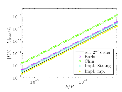
(a) Relative error of invariant $I$.

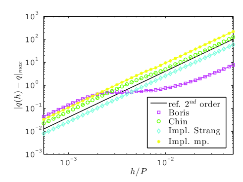
(b) Absolute error of position $q$.

Figure 1: 2d inhomogeneus magnetic field: maximum error (along trajectory) of the invariant $I$ and the position $q$ as a function of the time step length $h$ (in units of the analytic period length $P$) for a fixed total simulation time of $20000\,P$.

The error behavior becomes more visible when considering separately the error of the drift velocity and the error of the period length as shown in Figures 2a and 2b. The Boris pusher is the best method regarding the conservation of the drift velocity but the worst regarding the period length.

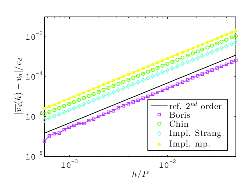
(a) Relative error of average drift velocity $\overline{v_{d}}$.

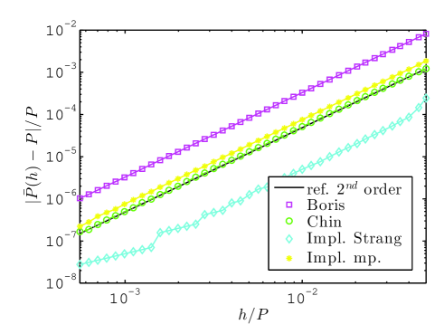
(b) Relative error of average period length $\bar{P}$.

Figure 2: 2d inhomogeneus magnetic field: error of the average drift velocity $\overline{v_{d}}$ and period length $\bar{P}$ as a function of the time step length $h$ (in units of the analytic period length $P$) for a fixed total simulation time of $20000\,P$.

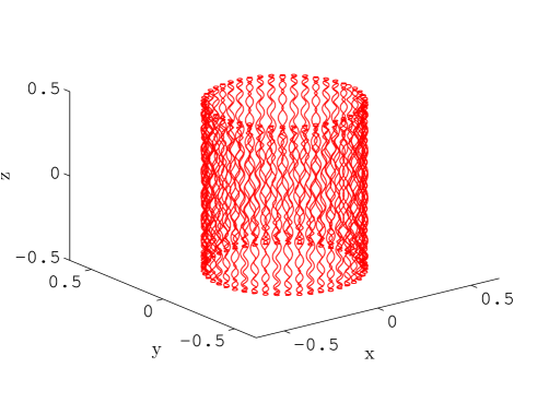
(a) Uniform magnetic field.

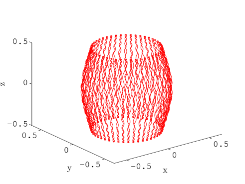
(b) Magnetic bottle.

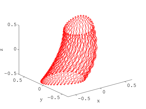
(c) Asymmetric magnetic field.

Figure 3: Particle trajectories for the three variations of the Penning trap.

VI.2 Ideal Penning trap with uniform magnetic field

The ideal Penning trap consists of a static quadrupole electric field and a uniform magnetic field given by

$$E =\kappa\begin{bmatrix}x&y&-2z\end{bmatrix}^{{\sf T}},$$ (35)

$$b =\begin{bmatrix}0&0&b_{z}\end{bmatrix}^{{\sf T}},$$

where $\kappa$ depends on the geometry and the voltage of the electrodes. The analytic solution for the motion of a single particle in an ideal Penning trap can be found in Kretzschmar . Choosing the trap parameters suitably gives a stable periodic orbit consisting of a fast gyromotion perpendicular to $b$ with the frequency $\omega_{mc}\approx\omega_{c}=\tfrac{c}{m}b_{z}$, a slower axial motion along $b$ with the frequency $\omega_{z}=\sqrt{2\frac{c}{m}\kappa}$ solely caused by the electrostatic fields and an even slower circular $E\times B$ drift motion around the $z$-axis with the magnetron frequency $\omega_{m}$. We set $c=1$, $m=1$, $b_{z}=100$, $\kappa=10$ and the initial coordinates of the particle $q_{0}=\begin{bmatrix}\tfrac{1}{3}&0&\tfrac{1}{2}\end{bmatrix}^{{\sf T}}$ and $p_{0}=\begin{bmatrix}0&1&0\end{bmatrix}^{{\sf T}}$. The particle trajectory of this example is shown in Figure 3a.

As the magnetic field is uniform in space the central step of the symmetric Hamiltonian splitting (26) can be computed exactly as is done in Scovel’s method. We compare this method to the method of Chin (25), the method of Spreiter and Walter (denoted by SpW), the Boris pusher (20) and its matrix exponential variation (21) (denoted by Boris exp).

We compare the methods by their ability to deliver a stable orbit over a large number of magnetron cycles (full circles around the $z$-axis), by the relative energy error (Figure 4a) and by the absolute error of the position (Figure 4b). As both types of errors are heavily oscillating, the maximum value of the error along a trajectory with a total simulation time of $2\pi\omega_{m}^{-1}$ (a complete magnetron cycle) is plotted against the time step length, using logarithmic scales for both quantities. The time step size ranges from 0.002 to 2.4 cyclotron cycles $f_{c}^{-1}=\tfrac{2\pi}{\omega_{c}}$, violating the stability criteria for some methods. A further reference line with a slope corresponding to a second-order method has been added to both plots.

With the exception of Spreiter and Walter all methods feature a bounded energy error and a position error increasing linearly in time on a closed orbit, as long as the time step size is considerably smaller than $f_{c}^{-1}$. The method of Spreiter and Walter shows a linearly increasing energy error until its orbit becomes unstable, so with longer simulation time its errors become worse relative to the other methods.

For larger time steps the method of Chin, the Hamiltonian splitting (Scovel) and the Boris pusher in its matrix exponential variation become unstable for $f_{c}h\approx n$, $n$ integer, while the Boris pusher using the Cayley transform preserves a closed orbit and a bounded energy error.

The Boris pusher provides in both variations a smaller energy error than the method of Chin and the Hamiltonian splitting, but shows a larger position error for small time steps. Figure 4b demonstrates an interesting behavior of the Boris pusher: for a large range of time step sizes the maximum position error remains constant at $\Delta q=0.02$, the diameter of the gyromotion. This can be explained by the fact that the Boris pusher can reproduce the correct first-order gyrocenter drift motion ParkerBirdsall .

The position error of a stable trajectory is bounded by the maximum diameter of the closed orbit (approximately 1 in our example), which causes the cut-offs in Figures  4b,  6b, and  7b.

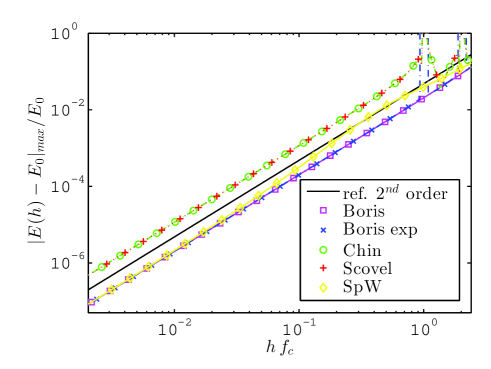
(a) Relative error of energy.

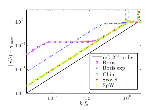
(b) Absolute error of position.

Figure 4: The ideal Penning trap: maximum error of the total energy $E$ and of the position $q$ along a trajectory of two complete magnetron cycles as a function of the time step size $h$ (in units of the inverse cyclotron frequency $f_{c}^{-1}$).

VI.3 Penning trap with magnetic bottle

The third experiment features a nonuniform magnetic field: a Penning trap with a magnetic bottle determined the magnetic field

$$b=b_{z}\begin{bmatrix}0&0&1\end{bmatrix}^{{\sf T}}+\beta\begin{bmatrix}-xz&-yz&z^{2}-\tfrac{x^{2}+y^{2}}{2}\end{bmatrix}^{{\sf T}}.$$ (36)

Here $E$ is as given in (35). A physical implementation of a Penning trap featuring such a magnetic field can be found in Rodegheri . We set $\beta=200$ and all the other parameters are as in the last example. The strength of the magnetic field and the cyclotron frequency $\omega_{c}$ vary only a little along the trajectory. The particle trajectory of this example is shown in Figure 3b.

When using the symmetric splitting method (26), approximations have to be made for the mid-step since now the magnetic field is nonuniform in space. Figure 5a shows the effect of the number of employed fixed-point iterations on the energy preservation of this method in a long time simulation of a trapped particle using a time step size of $h=0.4\,f_{c,0}^{-1}$, where $f_{c,0}$ is the cyclotron frequency at the initial position. As the position error is bounded by the closed orbit we choose the relative error of $\alpha$ (defined as the angle of motion around the $z$-axis) as a measure for the trajectory’s error in Figure 5b. Both errors are heavily oscillating, so the maximum value over each $10^{6}$ consecutive time steps is drawn.

The mid-step is either approximated by the implicit method (28) (denoted as Impl. Strang) or by (29) (denoted as Impl. mp.). For 5 fixed-point iterations (in the case of Impl. Strang) and 6 iterations (in the case of Impl. mp.) both alternatives seem to become approximately energy preserving and provide a stable orbit. This is expected from the theory, since the order of symmetry of these methods equals the number of fixed-point iterations employed EinkemmerOstermann and since a good long time behavior can be expected for symmetric methods HairerLubichWanner .

We compare the methods of Chin, the Boris pusher and the symmetric splitting method (26) using the implicit schemes as described above. Furthermore, we apply a high-order composition of (28) or (29) (denoted as Impl. mp. comp.). The composition is performed using an 8th-order symmetric scheme of Suzuki and Umeno SuzukiUmeno consisting of 15 substeps. Each substep uses 16 fixed-point iterations. Consequently, such a composition scheme requires a large number of magnetic field evaluations per time step: 240 for the method (29), or 255 when using the method (28) due to the calculation of the initial value within each substep. Nevertheless, a single electric field evaluation suffices for each time step. As the results of the implicit schemes do not differ considerably when the composition is applied, only the ones of (29) are drawn in the plots.

As before we provide two log-log plots showing the dependence of the energy and the position errors on the time step size in the range of 0.002 to 0.4 cyclotron cycles $f_{c,0}^{-1}$. Lacking an analytic solution to determine the position errors we use the trajectory of a high-order method with a small time step (0.00025 cyclotron cycles) as a reference: the fourth-order method of McLachlan applied on $\varphi_{h}^{\mathcal{T}}$ and $\varphi_{h}^{\mathcal{E}+\mathcal{B}}$ (denoted as M in Chin ) in combination with a composition scheme Suzuki_Fractals increasing the order to 6.

All variations of the symmetric Hamiltonian splitting method give an energy error similar to Chin’s scheme (Figure 6a). However, the smallest position error is obtained by using the composition scheme for the mid-step of the Hamiltonian splitting.

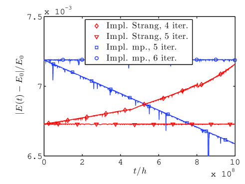
(a) Relative error of energy.

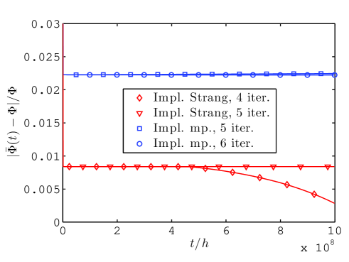
(b) Relative error of $\alpha$.

Figure 5: Penning trap (magnetic bottle): long time evolution of the errors of the total energy $E$ and the angle of circular motion $\alpha$ for different numbers of fixed-point iterations over $10^{9}$ time steps of fixed size $h=0.4f_{c}^{-1}$.

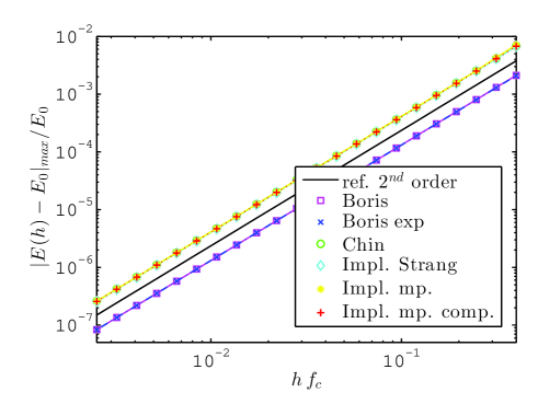
(a) Relative error of energy.

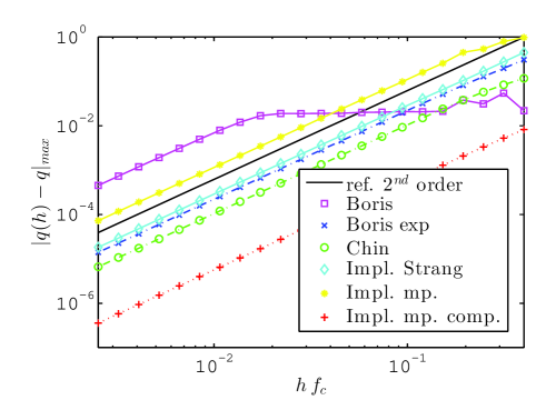
(b) Absolute error of position.

Figure 6: Penning trap (magnetic bottle): maximum error (along trajectory) of the total energy $E$ and of the position $q$ as a function of the time step size $h$ (in units of the inverse cyclotron frequency $f_{c}^{-1}$).

VI.4 Penning trap with asymmetric magnetic field

As the Penning trap with magnetic bottle is still rotationally invariant, we also consider an example with an asymmetric magnetic field given by

$$b(x,y,z)=b_{z}\begin{bmatrix}\tfrac{1}{3}&0&1\end{bmatrix}^{{\sf T}}+\beta\begin{bmatrix}y-z&x+z&y-x\end{bmatrix}^{{\sf T}},$$ (37)

where $\beta=50$. Notice that $\nabla\cdot b=\nabla\times b=0$. $E$ is again as given in (35). The particle trajectory of this example is shown in Figure 3c. Along the trajectory the magnetic field strength increases by a factor of 1.8. Therefore time step sizes between 0.001 and 0.1$f_{c,0}^{-1}$ are investigated in a simulation lasting for approximately 24 orbit cycles. Figures 7a and 7b show the energy and position errors for the methods giving similar results as in the previous example. The reference trajectory for the position errors has been computed with the method described in the previous example. Using the largest time step size $h=0.1f_{c,0}^{-1}$ shows unbounded energy errors for all the methods with the exception of the Boris pusher with the Cayley transform and the fixed point iteration schemes of the symmetric Hamiltonian splitting in combination with the high-order composition method of the mid-step. Therefore another long time integration over $2\cdot 10^{9}$ time steps of length 0.1$f_{c,0}^{-1}$ has been performed using both methods and the fourth-order method of McLachlan ; Chin (denoted by Chin M). For this example we measure also the magnetic moment defined by

$$\mu(q,p)=\frac{m}{2c^{2}}\frac{\|\Omega(q)p\|^{2}}{\|b(q)\|^{3}}=\frac{c}{2m^{2}}\frac{\|\Omega(q)p\|^{2}}{\omega_{c}^{3}}.$$

It is a so-called adiabatic invariant of the system HairerLubichWanner and should be conserved approximately. The magnetic moment as well as the energy error are oscillating within some range, so the maximum value on consecutive intervals of $10^{6}$ time steps is drawn in Figures 8a and 8b.

While the energy error of the Boris pusher remains smaller than that of the symmetric Hamiltonian splitting for over $4\cdot 10^{8}$ time steps, the evolution of the magnetic moment $\mu$ indicates the instability long before.

An initial decrease of $\mu$ is followed by a rapid growth after $3\cdot 10^{8}$ time steps for the Boris scheme. The Boris scheme with 2 times smaller time steps (denoted Boris h/2) shows a similar behavior with a delay. The fourth-order method denoted by Chin M exhibits a quickly growing error in energy but a smoother change of $\mu$. Only the symmetric Hamiltonian splitting in combination with a high-order approximation of the mid-step is able to provide a stable orbit.

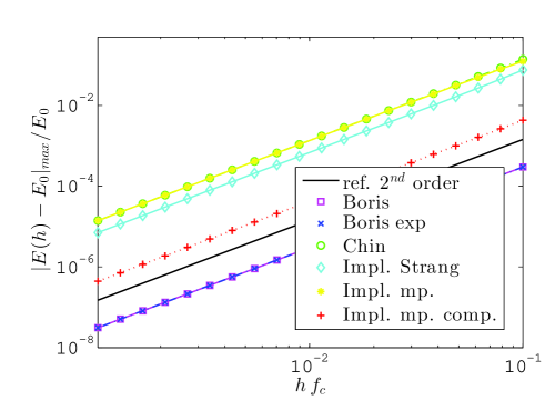
(a) Relative error of energy.

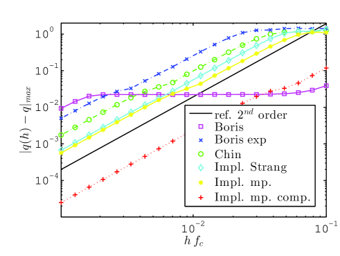
(b) Absolute error of position.

Figure 7: Penning trap (asymmetric field): maximum error (along trajectory) of the total energy $E$ and of the position $q$ as a function of the time step size $h$ (in units of the inverse cyclotron frequency $f_{c}^{-1}$).

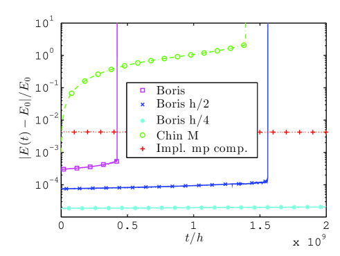
(a) Relative error of energy $E$.

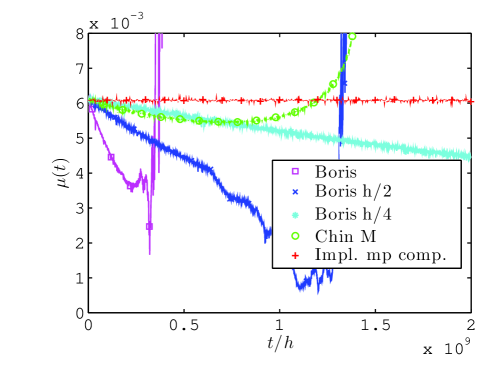
(b) Magnetic moment $\mu$.

Figure 8: Penning trap (asymmetric field): long time evolution of the magnetic moment $\mu$ and the error of the total energy $E$ over $2\cdot 10^{9}$ time steps of fixed size $h=0.1f_{c}^{-1}$.

VII Conclusions

We have considered here time integrators for particle trajectories in combined electric and magnetic fields. We have reformulated and analyzed existing methods found from literature under a common framework and additionally proposed a new method which deals the effect of the magnetic field implicitly. This is done by splitting the right-hand side of the equations of motion into three terms and by using the matrix function approach. The matrix functions are used for the magnetic field term, and the so-called Rodrigues formula simplifies their evaluation. We represent the equations of motion as a Poisson system and analyze the structure preserving properties of the integrators.

The existing methods we found in literature are: Boris–Buneman scheme, Chin’s schemes, the method of Spreiter and Walter, and the Scovel’s method. Additionally we have proposed a new implicit scheme. This scheme is the same as the Scovel’s method when the magnetic field is homogeneous.

The Boris–Buneman scheme and the Chin’s schemes are shown to be both symmetric and volume preserving. For the Spreiter and Walter’s scheme we did not find any structure preserving properties. The new method we propose is fully structure preserving up to an order equaling the number of fixed-point iterations used for the implicit mid-step. In numerical experiments we illustrate the effect of the number of fixed-point iterations on the preservation of the structure. In our experiments 6 iterations were enough to reduce the error negligible.

As a first numerical comparison, we tested all the schemes except Spreiter and Walter’s method in a case where there is no electric field. Due to the time symmetry, all the methods seemed to preserve invariants. For the position error the newly proposed implicit splitting method seemed to be the most accurate for small time steps, whereas for larger time steps the method of Boris was the most accurate. When the motion was separated into a periodic and a drift term, it was found that the method of Boris preserved the drift motion the best and the periodic motion the worst, whereas this was the opposite for the implicit splitting method.

To compare schemes in combined electric and magnetic fields, we integrated particle trajectories within a Penning trap. As the first example of combined fields we considered a constant homogeneous magnetic field, so Scovel’s method could be used producing energy and solution errors very similar to the method of Chin: a lower solution error than the Boris pusher for step-sizes considerably smaller than the inverse cyclotron frequency at the cost of a slightly larger but likewise bounded energy error. Spreiter and Walter’s method on the other hand did not feature a bounded energy error, so the orbit of the particle was unstable.

As a second Penning trap example we have an inhomogeneous but radially symmetric magnetic field. Replacing Scovel’s scheme by the new method still gave the same energy error like Chin’s scheme. The solution error differed depending on the method used for the implicit mid-step iteration. Applying a high order composition scheme on the mid-step provided the lowest solution error of all methods tested.

In the last numerical example of a Penning trap, we performed long time integration of a trajectory in an asymmetric magnetic field and compared three methods: one of the Chin’s schemes, the Boris–Buneman scheme and the newly proposed implicit method. We followed the preservation of the energy and of the magnetic moment. As expected from the analysis of Section V, the implicit method turned out to be the most stable. The Boris–Buneman scheme, being the second most stable, was more unstable than the implicit scheme even for 4 times smaller time steps.

VIII Appendix: Matrix functions

The following identities are easily verified for the skew-symmetric matrix $\Omega$ (see (4)):

$$\Omega^{2} =\omega\omega^{{\sf T}}-\omega_{c}^{2}I,$$

$$\Omega^{3} =-\omega_{c}^{2}\Omega,$$

where $\omega_{c}=\sqrt{\omega_{1}^{2}+\omega_{2}^{2}+\omega_{3}^{2}}$. Using the second identity and the Taylor series of $\sin$ and $\cos$, we get the Rodrigues formula for the exponential of $h\Omega$:

$$\exp{(h\Omega)}=I+\frac{\sin{h\omega_{c}}}{\omega_{c}}\Omega+\frac{1-\cos{h\omega_{c}}}{\omega_{c}^{2}}\Omega^{2}.$$ (38)

VIII.1 $\phi$ functions

We list here the necessary definitions and properties of the $\phi$ functions. These functions are defined by

$$\phi_{0}(z)={\rm e}\hskip 1.0pt^{z},\qquad\phi_{\ell}(z)=\int_{0}^{1}{\rm e}\hskip 1.0pt^{(1-\theta)z}\frac{\theta^{\ell-1}}{(\ell-1)!}\,{\rm d}\theta,\quad\ell\geq 1.$$ (39)

They satisfy $\phi_{\ell}(0)=\frac{1}{\ell!}$ and the recurrence relation

$$\phi_{\ell+1}(z)=\frac{\phi_{\ell}(z)-\phi_{\ell}(0)}{z},\quad\ell\geq 0.$$ (40)

The $\phi$ functions are analytic in the whole complex plane. Therefore, the matrix $\phi(A)$ is well defined for every $A\in\mathbb{C}^{n\times n}$. For various definitions and more details on matrix functions we refer to Higham . We mention that the $\phi$ functions play a crucial role also in the so-called exponential integrators HochbruckOstermann .

From (40) it follows that the series representation of the $\phi_{\ell}$ function is given by

$$\phi_{\ell}(z)=\sum_{j=0}^{\infty}\frac{z^{j}}{(j+\ell)!}.$$ (41)

We will also need the following formula, which can be easily verified using (41)

$$\phi_{\ell}\left(h\begin{bmatrix}0&\frac{1}{m}I\\ 0&\Omega\end{bmatrix}\right)=\begin{bmatrix}\tfrac{1}{\ell!}I&h\phi_{\ell+1}(h\Omega)\\ 0&\phi_{\ell}(h\Omega)\end{bmatrix},\quad\ell\geq 0.$$ (42)

Using the formula (38) and the integral definition (39), the following concise representations can be derived

$$\phi_{1}(h\Omega)=I +\frac{1-\cos(h\omega_{c})}{h\omega_{c}^{2}}\Omega+\frac{h\omega_{c}-\sin(h\omega_{c})}{h\omega_{c}^{3}}\Omega^{2},$$

$$\phi_{2}(h\Omega)=I +\frac{h\omega_{c}-\sin(h\omega_{c})}{h^{2}\omega_{c}^{3}}\Omega$$ (43)

$$+\left(\frac{\cos(h\omega_{c})-1}{h^{2}\omega_{c}^{4}}+\frac{1}{2\omega_{c}^{2}}\right)\Omega^{2}.$$

VIII.2 Variation-of-constants formula

The so-called variation-of-constants formula provides the solution of a semilinear ODE

$$y^{\prime}(t)=Ay(t)+g(t,y(t)),\quad y(0)=y_{0}.$$

It is given as

$$u(t)=\exp(tA)u_{0}+\int_{0}^{t}\exp\big{(}(t-\tau)A\big{)}\,g(\tau,u(\tau))\,{\rm d}\tau.$$ (44)

VIII.3 Relations for the Boris pusher

Let $\Omega$ be as in (4). An explicit calculation shows that

$$\big{(}I-\tfrac{h}{2}\Omega\big{)}^{-1}=I+\kappa\big{(}\tfrac{h}{2}\Omega+\tfrac{h^{2}}{4}\Omega^{2}\big{)},$$ (45)

where $\kappa=(1+\tfrac{h^{2}}{4}\omega_{c}^{2})^{-1}$ and $\omega_{c}=\sqrt{\omega_{1}^{2}+\omega_{2}^{2}+\omega_{3}^{2}}$. Multiplication by $I+\tfrac{h}{2}\Omega$ gives the Cayley transform of $\tfrac{h}{2}\Omega$,

$$R(\tfrac{h}{2}\Omega) =\big{(}I-\tfrac{h}{2}\Omega\big{)}^{-1}\big{(}I+\tfrac{h}{2}\Omega\big{)}$$ (46)

$$=I+2\kappa\big{(}\tfrac{h}{2}\Omega+\tfrac{h^{2}}{4}\Omega^{2}\big{)}.$$

The application of $R(\tfrac{h}{2}\Omega)$ on $p^{+}$ is equivalent to the cross product formulation of the Boris scheme (see BirdsallLangdon for the cross product formulation), since if

$$t =\tfrac{h}{2}\omega,$$

$$s =\tfrac{2t}{1+\|t\|^{2}}=\kappa h\omega,$$

$$p^{\prime} =p^{+}+p^{+}\times t=\big{(}I+\tfrac{h}{2}\Omega\big{)}p^{+},$$

then

$$p^{++} \,\,=p^{+}+p^{\prime}\times s,$$

$$\,\,=p^{+}+\big{(}(I+\tfrac{h}{2}\Omega)p^{+}\big{)}\times\kappa h\omega,$$

$$\,\,=p^{+}+2\kappa\tfrac{h}{2}\Omega\left(I+\tfrac{h}{2}\Omega\right)p^{+},$$

$$\,\,=\big{(}I+2\kappa(\tfrac{h}{2}\Omega+\tfrac{h^{2}}{4}\Omega^{2})\big{)}p^{+}.$$

References

- (1) C.K. Birdsall and A.B. Langdon, Plasma physics via computer simulation, CRC Press, 2005.
- (2) S.A. Chin, Symplectic and energy-conserving algorithms for solving magnetic field trajectories, Physical Review E 77.6 (2008), 066401.
- (3) L. Einkemmer and A. Ostermann, An almost symmetric Strang splitting scheme for the construction of high order composition methods, Journal of Computational and Applied Mathematics 271 (2014), pp. 307–318.
- (4) E. Hairer, C. Lubich and G. Wanner Geometric numerical integration. Structure-preserving algorithms for ordinary differential equations, 2nd ed., Springer, 2006.
- (5) N.J. Higham, Functions of matrices: theory and computation, SIAM, 2008.
- (6) M. Hochbruck and A. Ostermann, Exponential integrators, Acta Numerica 19 (2010), pp. 209–286.
- (7) A. Koskela and A. Ostermann, Exponential Taylor methods: analysis and implementation, Comput. Math. Appl., 65 (2013), pp. 487–499.
- (8) M. Kretzschmar, Single particle motion in a penning trap: description in the classical canonical formalism, European Journal of Physics 12.5 (1991), 240.
- (9) B. Leimkuhler and S. Reich, Simulating Hamiltonian dynamics, Vol. 14. Cambridge University Press, 2004.
- (10) H. Qin, S. Zhang, J. Xiao, J. Liu, Y. Sun, and W.M. Tang, Why is Boris algorithm so good?, Physics of Plasmas, 20(8) (2013), 084503.
- (11) Q. Spreiter and M. Walter Classical molecular dynamics simulation with the velocity Verlet algorithm at strong external magnetic fields, Journal of Computational Physics 152.1 (1999), pp. 102–119.
- (12) L. Patacchini and I.H. Hutchinson, Explicit time-reversible orbit integration in particle in cell codes with static homogeneous magnetic field, Journal of Computational Physics 228 (2009), pp. 2604–2614.
- (13) C.C. Rodegheri, An experiment for the direct determination of the g-factor of a single proton in a Penning trap, New Journal of Physics 14 (2012), 063011.
- (14) M. Suzuki and K. Umeno, Higher-order decomposition theory of exponential operators and its applications to QMC and nonlinear dynamics, Computer Simulation Studies in Condensed-Matter Physics VI (1993), Springer Proceedings in Physics 76, pp. 74–86.
- (15) M. Suzuki, Fractal decomposition of exponential operators with applications to many-body theories and Monte Carlo simulations, Physics Letters A 146 (1990), pp. 319–323.
- (16) R.I. McLachlan, On the numerical integration of ordinary differential equations by symmetric composition methods, SIAM Journal of Scientific Computing 16 (1995), pp. 151–168.
- (17) S.E. Parker and C.K. Birdsall, Numerical error in electron orbits with large , Journal of Computational Physics 97 (1991), pp. 91–102.