Stop Decay with LSP Gravitino in the final state: $\tilde{t}_{1}\rightarrow\,\widetilde{G}\,W\,b$

Abstract

In MSSM scenarios where the gravitino is the lightest supersymmetric particle (LSP), and therefore a viable dark matter candidate, the stop $\tilde{t}_{1}$ could be the next-to-lightest superpartner (NLSP). For a mass spectrum satisfying: $m_{\widetilde{G}}+m_{t}>m_{\tilde{t}_{1}}>m_{\widetilde{G}}+m_{b}+m_{W}$, the stop decay is dominated by the 3-body mode $\tilde{t}_{1}\rightarrow b\,W\,\tilde{G}$. We calculate the stop life-time, including the full contributions from top, sbottom and chargino as intermediate states. We also evaluate the stop lifetime for the case when the gravitino can be approximated by the goldstino state. Our analytical results are conveniently expressed using an expansion in terms of the intermediate state mass, which helps to identify the massless limit. In the region of low gravitino mass ($m_{\widetilde{G}}\ll m_{\tilde{t}_{1}}$) the results obtained using the gravitino and goldstino cases turns out to be similar, as expected. However for higher gravitino masses $m_{\widetilde{G}}\lesssim m_{\tilde{t}_{1}}$ the results for the lifetime could show a difference of O(100)%.

1 Introduction

The properties of Supersymmetric theories, both in the ultraviolet or the infrared domain have had a great impact in distinct domains of particle physics, including model building, phenomenology, cosmology and formal quantum field theory [1]. In particular, Supersymmetric extensions of the Standard Model can include a discrete symmetry, $R$ parity, that guarantees the stability of the lightest supersymmetric particle (LSP) [2], which allows the LSP to be a good candidate for dark matter (DM). Candidates for the LSP in the minimal supersymmetric extension of the Standard Model (MSSM) include sneutrinos, the lightest neutralino $\chi^{0}_{1}$ and the gravitino ${\widetilde{G}}$. Most studies has focused on the neutralino LSP [3], while scenarios with the sneutrino LSP seem more constrained  [4].

Scenarios with gravitino LSP as DM candidate have also been considered [5, 7, 6]. In such scenarios, the nature of the next-to-lightest supersymmetric particle (NLSP) determines its phenomenology [8, 9].

Possible candidates for NLSP include the lightest neutralino [10, 11], the chargino [12], the lightest charged slepton [13], or the sneutrino [14, 15, 16, 17]. The NLSP could have a long lifetime, due to the weakness of the gravitational interactions, and this leads to scenarios with a metastable charged sparticle that could have dramatic signatures at colliders [18, 19] and it could also affect the Big Bang nucleosynthesis (BBN) [20, 21, 22].

Squark species could also be the NLSP, and in such case natural candidates for NLSP could be the sbottom [23, 24, 25] or the lightest stop $\tilde{t}_{1}$. There are several experimental and cosmological constraints for the scenarios with a gravitino LSP and a stop NLSP that were discussed in [26]. It turns out that the lifetime of the stop ${\tilde{t}_{1}}$ could be (very) long, in which case the relevant collider limits are those on (apparently) stable charged particles. For instance the limits available from the Tevatron collider imply that $m_{\tilde{t}_{1}}>220$ GeV [27] . Thus, knowing in a precise way the stop lifetime is one of the most important issues in this scenario, and this is precisely the goal of our work. In this paper we present a detailed calculation of the stop lifetime, for the kinematical region where the 3-body mode $\tilde{t}_{1}\rightarrow\,\widetilde{G}\,W\,b$ dominates. Besides calculating the amplitude using the full wave function for the gravitino, we have also calculated the 3-body decay width (and lifetime) using the gravitino-goldstino equivalence theorem [28]. It should be mentioned that this scenario is not viable within the Constrained Minimal Supersymmetric Standard Model (CMSSM). However there are regions of parameter space within the Non-Universal Higgs Masses model (NUHM) that pass all collider and cosmological constraints (relic density, nucleosynthesis, CMB mainly) [29].

The organization of our paper goes as follows, we begin Section 2 by giving some formulae for the stop mass. In Section 2.1 we compute the squared amplitudes for the stop decay with gravitino in the final state ($\tilde{t}_{1}\rightarrow\,\widetilde{G}\,W\,b$) including the chargino, sbotom and top mediated states. After carefully analyzing the results for the squared amplitude, we have identified a convenient expansion in terms of powers of the intermediate particle mass, which only needs terms of order $O(m_{i}),\,O(m_{i}m_{j})$. It is our hope that such expansion could help in order to relate the calculation of the massive and massless cases. In future work we plan to reevaluate this decay using the helicity formalism suited for the spin-$\frac{3}{2}$ case. In Section 2.2 we compute the squared amplitudes for the stop decay considering the gravitino-goldstino high energy equivalence theorem that allow us approximate the gravitino as the derivative of the goldstino. We present in Section 3 our numerical results, showing some plots where we reproduce the stop lifetime for the approximate amplitude considered in [26], and compare it with our complete calculation, we also compare these results with goldstino approximation. Conclusions are included in Section 4, finally all the analytic full results for the squared amplitudes are left in Appendices A,B.

2 The Stop Lifetime within the MSSM

We start by giving some relevant formulae for the input parameters that appear in the Feynman rules of the gravitino within the MSSM. The (2x2) stop mass matrix can be written as:

$$\widetilde{M}_{\tilde{t}}^{2}=\begin{pmatrix}M_{LL}^{2}&M_{LR}^{2}\\ M_{LR}^{2\,{\dagger}}&M_{RR}^{2}\\ \end{pmatrix},$$ (1)

where the entries take the form:

$$M_{LL}^{2} =M_{L}^{2}+m_{t}^{2}+\frac{1}{6}\cos 2\beta\,(4m_{W}^{2}-m_{Z}^{2}),$$

$$M_{RR}^{2} =M_{R}^{2}+m_{t}^{2}+\frac{2}{3}\cos 2\beta\sin^{2}\theta_{W}\,m_{Z}^{2},$$ (2)

$$M_{LR}^{2} =-m_{t}(A_{t}+\mu\,\cot\beta)\equiv-m_{t}X_{t}\,.$$

The corresponding mass eigenvalues are given by:

$$m^{2}_{\tilde{t}_{1}}=m_{t}^{2}+\frac{1}{2}(M_{L}^{2}+M_{R}^{2})+\frac{1}{4}m^{2}_{Z}\cos 2\beta-\frac{\Delta}{2},$$ (3)

and

$$m^{2}_{\tilde{t}_{2}}=m^{2}_{t}+\frac{1}{2}(M_{L}^{2}+M_{R}^{2})+\frac{1}{4}m^{2}_{Z}\cos 2\beta+\frac{\Delta}{2},$$ (4)

where $\Delta^{2}=\left(M_{L}^{2}-M_{R}^{2}+\frac{1}{6}\cos 2\beta(8m^{2}_{W}-5m^{2}_{Z})\right)^{2}+4\,m_{t}^{2}|A_{t}+\mu\cot\beta|^{2}$. The mixing angle $\theta_{\tilde{t}}$ appears in the mixing matrix that relate the weak basis $(\tilde{t}_{L},\tilde{t}_{R})$ and the mass eigenstates $(\tilde{t}_{1},\tilde{t}_{2})$, and it is given by $\tan\theta_{\tilde{t}}=\frac{(m^{2}_{\tilde{t}_{1}}-M^{2}_{LL})}{|M^{2}_{LR}|}$. From these expressions it is clear that in order to obtain a very light stop one needs to have a very large value for the trilinear soft supersymmetry-breaking parameter [25, 30]. It turns out that such scenario helps to obtain a Higgs mass value in agreement with the mass measured at LHC (125-126 GeV) in a consistent way within the MSSM.

Following Ref. [31], we derived the expressions for all the relevant interactions vertices that appear in the amplitudes for the decay width ($\tilde{t}_{1}\rightarrow\,\widetilde{G}\,W\,b$), whose Feynman graphs are shown in Figures [1-3]. We shall need the following vertices:

$$V_{1}(\tilde{t}_{1}\,t\,\widetilde{G}) =-\frac{1}{\sqrt{2}M}(\gamma^{\nu}\gamma^{\mu}p_{\nu})(\cos\theta_{\tilde{t}}P_{R}+\sin\theta_{\tilde{t}}P_{L}),$$ (5)

$$V_{2}(t\,b\,W) =\frac{ig_{2}}{\sqrt{2}}\gamma_{\rho}P_{L},$$ (6)

$$V_{3}(\tilde{t}_{1}\,W\,\tilde{b}_{i}) =-\frac{ig_{2}\kappa_{i}}{\sqrt{2}}(p+q_{1})_{\mu}\,,$$ (7)

$$V_{4}(\tilde{b}_{i}\,b\,\widetilde{G}) =-\frac{1}{\sqrt{2}M}(\gamma^{\nu}\gamma^{\mu}q_{2\nu})(a_{i}P_{R}+b_{i}P_{L}),$$ (8)

$$V_{5}(\tilde{t}_{1}\,b\,\chi_{i}^{+}) =-i(S_{i}+P_{i}\gamma_{5}),$$ (9)

$$V_{6}(\chi_{i}^{+}\,W\,\widetilde{G}) =-\frac{1}{\sqrt{2}M}\Big{(}-\frac{1}{4}\not{p}\gamma^{\rho}\gamma^{\mu}(V_{1i}P_{R}-U_{i1}P_{L})$$ (10)

$$\quad-m_{W}\gamma^{\nu}\gamma^{\mu}(V_{i2}\sin{\beta}P_{R}+U_{i2}\cos\beta P_{L})\Big{)},$$

where $\tilde{t}_{1}$ denotes the lightest stop, while $t$ is the top quark and $\widetilde{G}$ denotes the gravitino. With $b$ we denote the bottom quark, while $W$ is the gauge boson, $\chi_{i}^{+}$ denotes the chargino and $\tilde{b}_{i}$ is de sbottom. With $P_{R}$ and $P_{L}$ corresponding to the left and right projectors, $a_{i}\,b_{i},\,S_{i},\,P_{i}$ are defined in Appendices A, B, as well the mixing matrices $V_{1i}$, $U_{1i}$ that diagonalize the chargino factor.

For the case when the gravitino approximates to the goldstino state, the interaction vertices that will appear in the amplitudes for the decay width ($\tilde{t}_{1}\rightarrow\,G\,W\,b$) are the following:

$$\widetilde{V}_{1}(\tilde{t}_{1}\,t\,G) =\left(\frac{m_{t}^{2}-m_{\tilde{t}_{1}}^{2}}{2\sqrt{3}Mm_{\widetilde{G}}}\right)(\cos\theta_{\tilde{t}}P_{R}+\sin\theta_{\tilde{t}}P_{L}),$$ (11)

$$\widetilde{V}_{4}(\tilde{b}_{i}\,b\,G) =\left(\frac{m_{b}^{2}-m_{\tilde{b}_{i}}^{2}}{2\sqrt{3}Mm_{\widetilde{G}}}\right)(a_{i}P_{R}+b_{i}P_{L}),$$ (12)

$$\widetilde{V}_{6}(\chi_{i}^{+}\,W\,G) =-\frac{m_{\chi_{i}^{+}}}{\sqrt{6}Mm_{\widetilde{G}}}[\not{p}\gamma^{\rho}(V_{1i}P_{R}-U_{i1}P_{L})],$$ (13)

whereas the vertices $V_{2}(t\,b\,W),\,V_{3}(\tilde{t}_{1}\,W\,\tilde{b}_{i})$ and $V_{5}(\tilde{t}_{1}\,b\,\chi_{i}^{+})$ remain the same as in the gravitino case.

2.1 The Amplitude for $\tilde{t}_{1}\rightarrow\,\widetilde{G}\,W\,b$

The decay lifetime of the stop was calculated in Ref.[26], where the chargino contribution was approximated by including only the dominant term. Here we shall calculate the full amplitude and determine the importance of the neglected term for the numerical calculation of the stop lifetime. In what follows we need to consider the Feynman diagrams shown in Figures [1,2,3], which contribute to the decay amplitude for $\tilde{t}_{1}(p)\rightarrow\,\widetilde{G}(p_{1})\,W(k)\,b(p_{2})$, with the momenta assignment shown in parenthesis.

Figure 1: Top mediated diagram

Figure 2: Sbottom mediated diagram

Figure 3: Chargino mediated diagram

The total amplitude is given by:

$$\mathcal{M}=\mathcal{M}_{t}+\mathcal{M}_{\tilde{b}_{i}}+\mathcal{M}_{\chi_{i}^{+}}^{C}\,,$$ (14)

where $\mathcal{M}_{t},\,\mathcal{M}_{\tilde{b}_{i}},\,\mathcal{M}_{\chi_{i}^{+}}^{C}$ denotes the amplitudes for top, sbottom and chargino mediate diagrams, respectively. In the calculation of Ref. [26], the chargino-mediated diagram included only part of the vertex $V_{6}(\chi_{i}^{+}\,W\,\widetilde{G})$. Here, in order to keep control of the vertex $V_{6}$ and therefore $\mathcal{M}_{\chi_{i}^{+}}^{c}$, we shall split $\mathcal{M}_{\chi_{i}^{+}}^{c}$ into two terms as follows

$$\mathcal{M}_{\chi_{i}^{+}}^{c}=\mathcal{M}_{\chi_{i}^{+}}^{0}+\mathcal{\widetilde{M}}_{\chi_{i}^{+}}\,,$$ (15)

where $\mathcal{M}_{\chi_{i}^{+}}^{0}$ denotes the amplitude considered in Ref. [26], which only includes the second term of [10] (with two gamma matrices), while $\mathcal{\widetilde{M}}_{\chi_{i}^{+}}$ includes the first term (with 3 gamma matrices). Then, the averaged squared amplitude [14] becomes

$$\mid\overline{\mathcal{M}}\mid^{2} =\mid\mathcal{M}_{t}\mid^{2}+\mid\mathcal{M}_{\tilde{b}_{i}}\mid^{2}+\mid\mathcal{M}_{\chi_{i}^{+}}^{0}\mid^{2}+\mid\mathcal{\widetilde{M}}_{\chi_{i}^{+}}\mid^{2}+2\,\textbf{Re}\Big{(}\mathcal{M}_{\chi_{i}^{+}}^{0\,\dagger}\mathcal{\widetilde{M}}_{\chi_{i}^{+}}+\mathcal{M}_{t}^{\dagger}\mathcal{M}_{\tilde{b}_{i}}$$

$$\quad+\mathcal{M}_{t}^{\dagger}\mathcal{M}_{\chi_{i}^{+}}^{0}+\mathcal{M}_{t}^{\dagger}\mathcal{\widetilde{M}}_{\chi_{i}^{+}}+\mathcal{M}_{\tilde{b}_{i}}^{\dagger}\mathcal{M}_{\chi_{i}^{+}}^{0}+\mathcal{M}_{\tilde{b}_{i}}^{\dagger}\mathcal{\widetilde{M}}_{\chi_{i}^{+}}\Big{)}.$$ (16)

From the inclusion of the vertices $V_{i}$ from each graph, we can build each amplitudes, as follows:

$$\mathcal{M}_{t} =C_{t}P_{t}(q_{1})\,\overline{\Psi}_{\mu}p^{\mu}(A_{t}+B_{t}\gamma_{5})(\not{q_{1}}+m_{t})\gamma^{\rho}\epsilon_{\rho}(k)P_{L}u(p_{2}),$$ (17)

$$\mathcal{M}_{\tilde{b}_{i}} =C_{\tilde{b}_{i}}P_{\tilde{b}_{i}}(q_{2})\,\overline{\Psi}_{\mu}q_{2}^{\mu}(a_{i}P_{l}+b_{i}P_{R})p^{\rho}\epsilon_{\rho}(k)P_{L}u(p_{2}),$$ (18)

$$\mathcal{M}_{\chi_{i}^{+}}^{0} =C_{\chi_{i}^{+}}^{0}P_{\chi_{i}^{+}}(q_{3})\,\overline{\Psi}_{\mu}\gamma^{\rho}\epsilon_{\rho}(k)\gamma^{\mu}(V_{i}+\Lambda_{i}\gamma_{5})(\not{q_{3}}+m_{\chi})(S_{i}+P_{i}\gamma_{5})u(p_{2}),$$ (19)

$$\mathcal{\widetilde{M}}_{\chi_{i}^{+}} =C_{\chi_{i}^{+}}P_{\chi_{i}^{+}}\overline{\Psi}_{\mu}\not{p}\gamma^{\rho}\gamma^{\mu}(T_{i}+Q_{i}\gamma_{5})\epsilon_{\rho}(k)(\not{q}_{3}+m_{\chi})(S_{i}+P_{i}\gamma_{5})u(p_{2}).$$ (20)

Where $C_{t}=\frac{g_{2}}{2M}$, $C_{\tilde{b}_{i}}=\frac{g_{2}\kappa_{i}}{M}$, $C_{\chi_{i}^{+}}^{0}=\frac{m_{W}}{M}$ and $C_{\chi_{i}^{+}}=\frac{1}{8M}$. We have defined $q_{1}\equiv p-p_{1},\,q_{2}\equiv p-k$ and $q_{3}\equiv p-p_{2}$, and $\epsilon_{\rho}(k)$ denotes the $W$ polarization vector. Expressions for $A_{\tilde{t}},B_{\tilde{t}},a_{i},b_{i},\kappa_{i},V_{i},A_{i},S_{i}$ and $P_{i}$ are presented in the Appendices A,B. Then, after performing the evaluation of each expression, we find convenient to express each squared amplitude, as follows:

$$\mid\mathcal{M}_{\psi_{a}}\mid^{2}=C_{\psi_{a}}^{2}\mid P_{\psi_{a}}(q_{a})\mid^{2}W_{\psi_{a}\psi_{a}},$$ (21)

where $\psi_{a}=(t,\tilde{b}_{j},\chi_{k}^{+})$. The functions $P_{\psi_{a}}(q_{a})$ correspond to the propagators factors, thus for the chargino $\psi_{a}=\chi_{i}^{+}$, we have

$$P_{\chi_{i}^{+}}(q_{3})=\frac{1}{q_{3}^{2}-m_{\chi_{i}^{+}}^{2}+i\epsilon}.$$ (22)

Similar expressions hold for the sbottom and the top contributions, $P_{\tilde{b}}(q_{2})$ and $P_{t}(q_{1})$ respectively. The terms $W_{\psi_{a}\psi_{a}}$ include the traces involved in each squared amplitudes

$$W_{tt} =\mathbf{Tr}\Big{[}M_{\rho\sigma}D_{\mu\nu}p^{\mu}p^{\nu}(A_{\tilde{t}}+B_{\tilde{t}}\gamma_{5})(\not{q}_{1}+m_{t})\gamma^{\rho}$$

$$\quad P_{L}\not{p}_{2}P_{R}\gamma^{\sigma}(\not{q}_{1}+m_{t})(A_{\tilde{t}}-B_{\tilde{t}}\gamma_{5})\Big{]},$$ (23)

$$W_{\tilde{b}_{i}\tilde{b}_{i}} =\mathbf{Tr}\Big{[}p^{\rho}p^{\sigma}M_{\rho\sigma}D_{\mu\nu}q_{2}^{\mu}q_{2}^{\nu}(R_{i}+Z_{i}\gamma_{5})\not{p_{2}}(R_{j}-Z_{j}\gamma_{5})\Big{]},$$ (24)

$$W_{\chi_{i}^{+}\chi_{i}^{+}}^{0} =\mathbf{Tr}\Big{[}M_{\rho\sigma}D^{\rho\sigma}(V_{i}+\Lambda_{i}\gamma_{5})(\not{q_{3}}+m_{\chi})(S_{i}+P_{i}\gamma_{5})\not{p}_{2}$$ (25)

$$\quad(S_{j}-P_{j}\gamma_{5})(\not{q_{3}}+m_{\chi})(V_{j}-\Lambda_{j}\gamma_{5})\Big{]},$$

$$W_{\chi_{i}^{+}\chi_{i}^{+}} =\mathbf{Tr}\Big{[}M_{\rho\sigma}D_{\mu\nu}\not{p}\gamma^{\rho}\gamma^{\mu}(T_{i}+Q_{i}\gamma_{5})(\not{q}_{3}+m_{\chi})(S_{i}+P_{i}\gamma_{5})\not{p}_{2}(S_{j}-P_{j}\gamma_{5})$$ (26)

$$\quad(\not{q}_{3}+m_{\chi})(T_{j}-Q_{j}\gamma_{5})\gamma^{\nu}\gamma^{\sigma}\not{p}\Big{]}.$$

For simplicity, we have written the completeness relations for the gravitino field and the vector polarization sum of the boson W as follows:

$$\sum_{\lambda=1}^{3}\epsilon_{\rho}(\vec{k},\lambda)\epsilon_{\sigma}^{*}(\vec{k},\lambda) =-g_{\rho\sigma}+\frac{k_{\rho}k_{\sigma}}{m_{W}^{2}}=M_{\rho\sigma}$$ (27)

$$\sum_{\tilde{\lambda}=1}^{3}\Psi_{\mu}(\vec{p}_{1},\tilde{\lambda})\overline{\Psi}_{\nu}(\vec{p}_{1},\tilde{\lambda}) =-(\not{p}_{1}+m_{\tilde{G}})\times\left\{\left(g_{\mu\nu}-\frac{p_{\mu}p_{\nu}}{m_{\tilde{G}}^{2}}\right)\right.$$ (28)

$$\quad\left.-\frac{1}{3}\Bigg{(}g_{\mu\sigma}-\frac{p_{\mu}p_{\sigma}}{m_{\tilde{G}}^{2}}\Bigg{)}\Bigg{(}g_{\nu\lambda}-\frac{p_{\nu}p_{\lambda}}{m_{\tilde{G}}^{2}}\Bigg{)}\gamma^{\sigma}\gamma^{\lambda}\right\}=D_{\mu\nu}.$$ (29)

The functions $W_{\psi_{a}\psi_{a}}$ depend on the scalar products of the momenta $p,p_{1},p_{2},k,q_{1},q_{2}$ and $q_{3}$. After carefully analyzing the resulting traces (handed with FeynCalc [37, 38]) we find that these functions can be written as powers of the intermediate state masses, as follows:

$$W_{\psi_{a}\psi_{a}}=\text{w}_{1\psi_{a}\psi_{a}}+m_{\psi_{a}}\text{w}_{2\psi_{a}\psi_{a}}+m_{\psi_{a}}^{2}\text{w}_{3\psi_{a}\psi_{a}}.$$ (30)

Full expressions for each function $\text{w}_{i\psi_{a}\psi_{a}}$ $\forall\,i=1,2,3$ are included in Appendix A. Furthermore, we also find that the interference terms can be written in a similar form, namely:

$$\mathcal{M}_{\psi_{a}}^{\dagger}\mathcal{M}_{\psi_{b}}=C_{\psi_{a}}C_{\psi_{b}}P^{*}_{\psi_{a}}(q_{a})P_{\psi_{b}}(q_{b})W_{\psi_{a}\psi_{b}}.$$ (31)

Again, as in the previous case, the function $W_{\psi_{a}\psi_{b}}$ include the traces appearing in the interferences, specifically we have

$$\widetilde{W}_{\chi_{i^{+}}\chi_{i^{+}}} =\mathbf{Tr}\Big{[}M_{\rho\sigma}D_{\mu\nu}\not{p}\gamma^{\rho}\gamma^{\mu}(T_{i}+Q_{i}\gamma_{5})(\not{q}_{3}+m_{\chi})\not{p}_{2}(S_{i}-P_{i}\gamma_{5})(S_{j}-P_{j}\gamma_{5})$$ (32)

$$\quad(\not{q}_{3}+m_{\chi})(V_{j}-\Lambda_{j}\gamma_{5})\gamma^{\nu}g^{\sigma}\Big{]},$$

$$W_{t\tilde{b}_{i}} =\mathbf{Tr}\Big{[}M_{\rho\sigma}p^{\rho}\not{p}_{2}P_{R}\gamma^{\sigma}(\not{q}_{1}+m_{t})(A_{\tilde{t}}-B_{\tilde{t}}\gamma_{5})p^{\mu}D_{\mu\nu}q_{2}^{\nu}(R_{i}+Z_{i}\gamma_{5})\Big{]},$$ (33)

$$W_{t\chi_{i}^{+}} =\mathbf{Tr}\Big{[}M_{\rho\sigma}\not{p}_{2}P_{R}\gamma^{\sigma}(\not{q}_{1}+m_{t})(A_{\tilde{t}}-B_{\tilde{t}}\gamma_{5})p_{\mu}D^{\mu\rho}(\Lambda_{i}+V_{i}\gamma_{5})(\not{q}_{3}+m_{\chi})$$ (34)

$$\quad(S_{i}+P_{i}\gamma_{5})\Big{]},$$

$$\widetilde{W}_{t\chi_{i}^{+}} =\mathbf{Tr}\Big{[}M_{\rho\sigma}D_{\mu\nu}\not{p}\gamma^{\rho}\gamma^{\mu}p^{\nu}(T_{i}+Q_{i}\gamma_{5})(\not{q}_{3}+m_{\chi})(S_{i}+P_{i}\gamma_{5})\not{p}_{2}P_{R}\gamma^{\sigma}$$ (35)

$$\quad(\not{q}_{1}+m_{t})(A_{\tilde{t}}-B_{\tilde{t}}\gamma_{5})\Big{]},$$

$$W_{\chi_{i}^{+}\tilde{b}_{i}} =\mathbf{Tr}\Big{[}M_{\rho\sigma}p^{\rho}(p_{\nu}-k_{\nu})\not{p}_{2}(S_{i}-P_{i}\gamma_{5})(\not{q}_{3}+m_{\chi})(\Lambda_{i}-V_{i}\gamma_{5})$$ (36)

$$\quad D^{\nu\sigma}(R_{j}+Z_{j}\gamma_{5})\Big{]},$$

$$\widetilde{W}_{\chi_{i}^{+}\tilde{b}_{i}} =\mathbf{Tr}\Big{[}M_{\rho\sigma}D_{\mu\nu}(p^{\nu}-k^{\nu})(R_{i}+Z_{i}\gamma_{5})\not{p}_{2}(S_{i}-P_{i}\gamma_{5})(\not{q}_{3}+m_{\chi})$$ (37)

$$\quad(T_{i}-Q_{i}\gamma_{5})\gamma^{\mu}\gamma^{\rho}\not{p}p^{\sigma}\Big{]}.$$

It turns out that the functions $W_{\psi_{a}\psi_{b}}$ can be expressed also in powers of the intermediate masses:

$$W_{\psi_{a}\psi_{b}}=\text{w}_{1\psi_{a}\psi_{b}}+m_{\psi_{a}}(\text{w}_{2\psi_{a}\psi_{b}}+m_{\psi_{b}}\text{w}_{3\psi_{a}\psi_{b}})+m_{\psi_{b}}\text{w}_{4\psi_{a}\psi_{b}}.$$ (38)

The $\text{w}_{j\psi_{a}\psi_{b}}$ $\forall\,j=1,2,3,4$ are as the $\text{w}_{i\psi_{a}\psi_{a}}$ 4-momentum’s scalar products functions completely determined by the kinematics of our decay. We consider that [30] and [38] are an useful way to present our results as well an easy manner to compute complicated and messy traces. Then the decay width can be obtained after integration of the 3-body phase-space

$$\frac{d\Gamma}{dx\,dy}=\frac{m_{\tilde{t}_{1}}^{2}}{256\,\pi^{3}}\mid\overline{\mathcal{M}}\mid^{2}.$$ (39)

The variables $x$ and $y$ are defined as $x=2\frac{E_{\widetilde{G}}}{m_{\tilde{t}_{1}}}$ and $y=2\frac{E_{W}}{m_{\tilde{t}_{1}}}$. Numerical results for the lifetime $\tau=\frac{1}{\Gamma}$ will be presented and discussed in Section 3.

2.2 The Amplitudes $\tilde{t}_{1}\rightarrow\,G\,W\,b$ with the goldstino approximation

In this section we shall present the calculation of the stop decay using the gravitino-goldstino high energy equivalence theorem [28]. In the high energy limit ($m_{\widetilde{G}}\ll m_{\tilde{t_{1}}}$) we could consider the gravitino field (spin $\frac{3}{2}$ particle) as the derivative of the goldstino field (spin $\left(\frac{1}{2}\right)$ particle). We shall consider in this section the same Feynman diagrams Figures [1,2,3] that we used in Section 2.1, but with the proviso that the gravitino field shall be described by the goldstino fields. Making the replacement $\Psi_{\widetilde{G}}\to i\sqrt{\frac{2}{3}}\frac{1}{m_{\widetilde{G}}}\,\partial_{\mu}\Psi$ in the gravitino interaction lagrangian, one obtain the effective interaction lagrangian for the goldstino as is show in [31]. The averaged squared amplitude for the Goldstino is then written as

$$\mid\overline{\mathcal{M}^{G}}\mid^{2} =\mid\mathcal{M}_{t}^{G}\mid^{2}+\mid\mathcal{M}_{\tilde{b}_{i}}^{G}\mid^{2}+\mid\mathcal{M}_{\chi_{i}^{+}}^{G}\mid^{2}$$ (40)

$$\quad+2\,\textbf{Re}(\mathcal{M}_{t}^{G\,\dagger}\mathcal{M}^{G}_{\tilde{b}_{i}}+\mathcal{M}_{t}^{G\,\dagger}\mathcal{M}_{\chi_{i}^{+}}^{G}+\mathcal{M}_{\tilde{b}_{i}}^{G\,\dagger}\mathcal{M}_{\chi_{i}^{+}}^{G}).$$

As in the previous Section 2.1, we can build the amplitudes from the inclusion of all the vertices into the expressions from each graph, namely:

$$\mathcal{M}_{t}^{G} =\widetilde{C}_{t}P_{t}(q_{1})\overline{\Psi}(A_{\tilde{t}}+B_{\tilde{t}}\gamma_{5})(\not{q}_{1}+m_{t})\gamma^{\rho}P_{L}\epsilon_{\rho}(k)u(p_{2}),$$ (41)

$$\mathcal{M}_{\tilde{b}_{i}}^{G} =\widetilde{C}_{\tilde{b}_{i}}P_{\tilde{b}_{i}}(q_{2})\overline{\Psi}(R_{i}+Z_{i}\gamma^{5})u(p_{2})p^{\sigma}\epsilon_{\sigma}(k),$$ (42)

$$\mathcal{M}_{\chi_{i}^{+}}^{G} =\widetilde{C}_{\chi_{i}^{+}}P_{\chi_{i}^{+}}(q_{3})\not{p}\gamma^{\rho}(T_{i}+Q_{i}\gamma_{5})\overline{\Psi}\epsilon_{\rho}(k)(\not{q}_{3}+m_{\chi})(S_{i}+P_{i}\gamma_{5})u(p_{2}).$$ (43)

Where the superindex “G” that appears in the amplitudes [41-43] refers to the goldstino amplitudes. The constants appearing in front of each amplitudes are: $\widetilde{C}_{t}=-g_{2}\left(\frac{m_{t}^{2}-m_{\tilde{t}_{1}}^{2}}{4\sqrt{6}Mm_{\widetilde{G}}}\right)$, $\widetilde{C}_{\tilde{b}_{i}}=g_{2}\kappa_{i}\left(\frac{m_{b}^{2}-m_{\tilde{b}_{i}}^{2}}{4\sqrt{6}Mm_{\widetilde{G}}}\right)$ and $\widetilde{C}_{\chi_{i}^{+}}=-\frac{m_{\chi_{i}^{+}}}{\sqrt{6}Mm_{\widetilde{G}}}$. We obtain similar expressions to [LABEL:eq:71:amplitudes] for the squared amplitudes of the goldstino case, namely:

$$\mid\mathcal{M}_{\psi_{a}}^{G}\mid^{2}=\widetilde{C}_{\psi_{a}}^{2}\mid P_{\psi_{a}}(q_{a})\mid^{2}W_{\psi_{a}\psi_{a}}^{G},$$ (44)

where the function $W_{\psi_{a}\psi_{a}}^{G}$ includes traces corresponding to the goldstino squared amplitudes, which are given as follows:

$$W_{tt}^{G} =\mathbf{Tr}\Big{[}(\not{p}_{1}+m_{\tilde{G}})(A_{\tilde{t}}+B_{\tilde{t}}\gamma_{5})(\not{q}_{1}+m_{t})\gamma^{\rho}P_{L}M_{\rho\sigma}\not{p}_{2}$$ (45)

$$\quad P_{R}\gamma^{\sigma}(\not{q}_{1}+m_{t})(A_{\tilde{t}}-B_{\tilde{t}}\gamma_{5})\Big{]},$$

$$W^{G}_{\tilde{b}_{i}\tilde{b}_{i}} =\mathbf{Tr}\Big{[}p^{\rho}p^{\sigma}M_{\rho\sigma}(\not{p}_{1}+m_{\tilde{G}})(B_{i}+Z_{i}\gamma_{5})\not{p}_{2}(B_{j}-Z_{j}\gamma_{5})\Big{]},$$ (46)

$$W_{\chi_{i}^{+}\chi_{i}^{+}}^{G} =\mathbf{Tr}\Big{[}M_{\rho\sigma}(\not{p}_{1}+m_{\tilde{G}})\not{p}\gamma^{\rho}(T_{i}+Q_{i}\gamma_{5})(\not{q}_{3}+m_{\chi})(S_{i}+P_{i}\gamma_{5})\not{p}_{2}$$ (47)

$$\quad(S_{j}-P_{j}\gamma_{5})(\not{q}_{3}+m_{\chi})(T_{j}-Q_{j}\gamma_{5})\gamma^{\sigma}\not{p}\Big{]},$$

the functions $W_{\psi_{a}\psi_{a}}^{G}$ depend on the scalar products of the momenta $p,p_{1},p_{2},k,q_{1},q_{2}$ and $q_{3}$, these functions will also be written as powers of the intermediate state masses, namely:

$$W_{\psi_{a}\psi_{a}}^{G}=\text{w}_{1\psi_{a}\psi_{a}}^{G}+m_{\psi_{a}}\text{w}_{2\psi_{a}\psi_{a}}^{G}+m_{\psi_{a}}^{2}\text{w}_{3\psi_{a}\psi_{a}}^{G}.$$ (48)

All the full expressions for each function $\text{w}_{i\psi_{a}\psi_{a}}^{G}$ $\forall\,i=1,2,3$ can be foud in Appendix B. Again, the interferences terms for the goldstino are also written in the form:

$$\mathcal{M}_{\psi_{a}}^{G\,\dagger}\mathcal{M}_{\psi_{b}}^{G}=\widetilde{C}_{\psi_{a}}\widetilde{C}_{\psi_{b}}P^{*}_{\psi_{a}}(q_{a})P_{\psi_{b}}(q_{b})W_{\psi_{a}\psi_{b}}^{G}.$$ (49)

The functions $W_{\psi_{a}\psi_{b}}$ correspond to the traces involved in the interference terms, i.e.

$$W_{t\tilde{b}_{i}}^{G} =\mathbf{Tr}\Big{[}M_{\rho\sigma}\not{p}_{2}P_{R}\gamma^{\sigma}(\not{q}_{1}+m_{t})(A_{\tilde{t}}-B_{\tilde{t}}\gamma_{5})(\not{p}_{1}+m_{\tilde{G}})(B_{i}+Z_{i}\gamma_{5})p^{\rho}\Big{]},$$ (50)

$$W_{t\chi_{i}^{+}}^{G} =\mathbf{Tr}\Big{[}M_{\rho\sigma}(\not{p}_{1}+m_{\tilde{G}})\not{p}\gamma^{\rho}(T_{i}+Q_{i}\gamma_{5})(\not{q}_{3}+m_{\chi})(S_{i}+P_{I}\gamma_{5})$$ (51)

$$\quad\not{p}_{2}P_{R}\gamma^{\sigma}(\not{q}_{1}+m_{t})(A_{\tilde{t}}-B_{\tilde{t}}\gamma_{5})\Big{]},$$

$$W_{\chi_{i}^{+}\tilde{b}_{i}}^{G} =\mathbf{Tr}\Big{[}M_{\rho\sigma}\not{p}_{2}(S_{i}-P_{i}\gamma_{5})(\not{q}_{3}+m_{\chi})(T_{i}-Q_{i}\gamma_{5})\gamma^{\rho}\not{p}(\not{p}_{1}+m_{\tilde{G}})(R_{j}+Z_{j}\gamma_{5})p^{\sigma}\Big{]}.$$ (52)

The $W_{\psi_{a}\psi_{b}}^{G}$ functions also expressed as powers of the intermediate masses:

$$W_{\psi_{a}\psi_{b}}=\text{w}_{1\psi_{a}\psi_{b}}^{G}+m_{\psi_{a}}(\text{w}_{2\psi_{a}\psi_{b}}^{G}+m_{\psi_{b}}\text{w}_{3\psi_{a}\psi_{b}}^{G})+m_{\psi_{b}}\text{w}_{4\psi_{a}\psi_{b}}^{G}.$$ (53)

The full expressions for $\text{w}_{j\psi_{a}\psi_{b}}^{G}$ $\forall\,j=1,2,3,4$ can be found in the Appendix B.

3 Numerical Results

The decay width is obtained by integrating the differential decay width over the dimensionless variables $x,\,y$ which have limits given by $2\mu_{G}<x<1+\mu_{\tilde{G}}-\mu_{W}$ with $\mu_{i}=\frac{m_{i}^{2}}{m_{\tilde{t}_{1}}^{2}}$ and

$$y_{\pm}=\frac{(2-x)\left(\mu_{\tilde{G}}+\mu_{W}-x+1\right)\pm\sqrt{x^{2}-4\mu_{\tilde{G}}}\left(\mu_{\tilde{G}}-\mu_{W}-x+1\right)}{2\left(\mu_{\tilde{G}}-x+1\right)},$$ (54)

$$\Gamma=\int_{2\mu_{G}}^{1+\mu_{G}-\mu_{W}}\int_{y_{-}}^{y_{+}}\frac{m_{\tilde{t}_{1}}^{2}}{256\,\pi^{3}}\mid\overline{\mathcal{M}}\mid^{2}dy\,dx.$$ (55)

After integrating numerically the expressions for the differential decay width, we obtain the values for the decay width, for a given set of parameters. We consider two values for the stop mass, $m_{\tilde{t}_{1}}=200\,GeV$ and $m_{\tilde{t}_{1}}=350\,GeV$, we also fix the chargino mass to be $m_{\chi_{i}^{+}}=200,\,500\,GeV$, while the sbottom mass is fixed to be $m_{\tilde{b}_{i}}=300,\,500\,GeV$.

In Figures [4,5] we show the lifetime of the stop, as function of the gravitino mass, within the ranges 200-250 GeV for the case with $m_{\tilde{t}_{1}}=350\,GeV$, and 50-100 GeV for $m_{\tilde{t}_{1}}=100\,GeV$. We show the results for the case when one uses the full expression for chargino-gravitino-W vertex (circles), as well as the case when the partial inclusion of such vertex, as it was done in [26] (triangles) and in the limit of the goldstino approximation (squares). We noticed that for low gravitino masses ($m_{\widetilde{G}}\to 0$) the full gravitino result becomes almost indistinguishable from the goldstino case, while the partial gravitino result has also similar behavior. For larges gravitino masses ($m_{\widetilde{G}}\cong m_{\tilde{t}_{1}}$) the results for the stop lifetime using the full gravitinio and goldstino approximation could be very different, up to $O(50\%)$ different.

On the other hand, the values for the stop life-time using the full gravitino and partial gravitino limit are very similar for low gravitino masses, while for the largest allowed masses the difference in results is at most of order $O(50\%)$. The value of the lifetime obtained in all theses cases turns out to be of order $10^{7}\,-\,10^{12}$ sec, which results in an scenario with large stop lifetime that has very special signatures both at colliders and has also important implications for cosmology, as it was discussed in ref. [26].

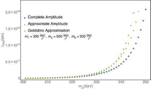
Figure 4: Stop lifetime 1

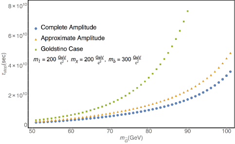
Figure 5: Stop lifetime 2

For instance, regarding the effect on BBN, the Stop $\tilde{t}_{1}$ have to form quasi stable sbaryons ($\tilde{t}_{1}qq$) and mesinos ($\tilde{t}_{1}\bar{q}$), whose late decays could have affected the light element abundance obtained in BBN, while negatively charged stop sbaryons and mesinos could contribute to lower the Coulomb barrier for nuclear fusion process occurring in the BBN epoch. However, as argued in [26] the great majority of stop antisbaryons would have annihilated with ordinary baryons to make stop antimesinos and most stop mesinos and antimesinos would have annihilated. The only remnant would have been neutral mesinos which would be relatively innocuous, despite their long lifetime because they would not have important bound state effects. Further discussion of BBN issues of Ref. [29] divide the stop lifetime into regions that could have an effect, but the larges ones (which represent our results) do not pose problems for the success of BBN. Then, regarding the effect of late stop decay on the Cosmic Microwave Background (CMB), we have included some comments in the text, to estimate the main effects. The arguments which read as follows: Very long lifetimes ($\tau>10^{12}\,s$) would have been excluded if one uses the approximate results of Ref. [39], which present bounds on the lifetime $\tau$ (for the case when stau is the NLSP) using the constrain in the chemical potential $\mu<9\times 10^{-5}$. However, it was discussed in Ref. [40], that a more precise calculation reduces the excluded region for lifetimes, ending at about $\tau\sim 10^{11}s-10^{12}s$. Thus, the region with very large stop lifetimes could also survive. Specific details that change from the stop decay (3-body) as compared with stau decays (2-body), such as the energy release or stop hadronization, will affect the calculation, but the numerical evaluation of such effect is beyond the scope of our paper.

4 Conclusions

In this paper we have calculated the stop $\tilde{t}_{1}$ lifetime in MSSM scenarios where the massive gravitino is the lightest supersymmetric particle (LSP), and therefore is a viable dark matter candidate. The lightest stop $\tilde{t}_{1}$ corresponds to the next-to-lightest supersymmetric particle (NLSP). We have focused on the kinematical domain $m_{\widetilde{G}}+m_{t}>m_{\tilde{t}_{1}}>m_{\widetilde{G}}+m_{b}+m_{W}$, where the stop decay width is dominated by the mode $\tilde{t}_{1}\rightarrow b\,W\,\tilde{G}$.

The amplitiude for the full calculation of the stop 3-body decay width includes contributions from top, sbottom and chargino as intermediate states. We have considered the full chargino-gravitino vertex, which improves the calculation presented in ref. [26]. Besides performing the full calculation with massive gravitino, we have also evaluated the stop decay lifetime for the limit when the gravitino can be approximated by the goldstino state. Our analytical results are conveniently expressed, in both cases, using an expansion in terms of the intermediate state mass, which helps in order to identify the massless limit.

We find that the results obtained with the full chargino vertex are not very different from the approximation used in ref. [26], in fact they only differ approximately in a 50%. The comparison of the full numerical results with the ones obtained for the goldstino approximation, show that in the limit of low gravitino mass ($m_{\widetilde{G}}\ll m_{\tilde{t}_{1}}$) there is not a significant difference in values of the stop life-time obatined from each method. However, for $m_{\widetilde{G}}\lesssim m_{\tilde{t}_{1}}$ the difference in lifetime could be as high as 50%. Numerical results for the stop lifetime give value of order $10^{7}\,-\,10^{12}$ sec, which makes the stop to behave like a quasi-stable state, which leaves special imprints for LHC search. Our calculation shows that the inclusion of the neglected term somehow gives a decrease in the lifetime of the stop. However, it should be pointed out that the region of parameter space correspond to the NUHM model.

Appendix A Analytical Expressions for Amplitudes with Gravitino in the final state

In this appendix we present explicitly the full results for the 10 $\text{w}_{\psi_{a}\psi_{a}}$ functions that arose from a convenient way to express the large traces that appear in the squared amplitudes [21], as well as the 18 $\text{w}_{\psi_{a}\psi_{b}}$ functions in the interferences [31] of the 3-body stop $\tilde{t}_{1}$ decay with gravitino in the final state. First, we shall present the contributions for the squared amplitudes, then we shall present the interferences.

A.1 Top Contribution

For the averaged squared amplitude of the top quark contribution, the functions $\text{w}_{1tt},\,\text{w}_{2tt}$ and $\text{w}_{3tt}$ are:

$$\text{w}_{1tt} =\frac{4a_{1}h_{1}}{3m_{W}^{2}m_{\tilde{G}}^{2}}\Bigl{(}f_{2}(m_{W}^{2}(6m_{\tilde{G}}^{2}+2h_{5}m_{\tilde{t}_{1}}^{2}-q_{1}^{2})+6f_{3}m_{W}^{2}+4f_{3}^{2})-2f_{1}\bigl{(}m_{\tilde{G}}^{2}\bigl{(}-\bigl{(}4f_{3}$$

$$\quad+3m_{W}^{2}\bigr{)}\bigr{)}+f_{2}(4f_{3}+3m_{W}^{2})+f_{3}q_{1}^{2}\bigr{)}+(q_{1}^{2}-2m_{\tilde{G}}^{2})(m_{W}^{2}m_{\tilde{G}}^{2}+3f_{3}m_{W}^{2}+2f_{3}^{2})$$

$$\quad+4f_{1}^{2}(f_{2}-m_{\tilde{G}}^{2})-2m_{W}^{2}m_{\tilde{G}}^{2}h_{5}m_{\tilde{t}_{1}}^{2}-4f_{2}^{2}m_{W}^{2}\Bigr{)},$$ (56)

$$\text{w}_{2tt} =\frac{8a_{2}h_{1}}{3m_{W}^{2}m_{\tilde{G}}}(m_{W}^{2}(m_{\tilde{G}}^{2}+m_{\tilde{t}}^{2}-2f_{2})-f_{1}(4f_{3}+3m_{W}^{2})+3f_{3}m_{W}^{2}+2f_{1}^{2}+2f_{3}^{2}),$$ (57)

$$\text{w}_{3tt} =\frac{4a_{3}h_{1}}{3m_{W}^{2}m_{\tilde{G}}^{2}}(m_{W}^{2}(f_{2}-m_{\tilde{G}}^{2})-3f_{3}m_{W}^{2}-2f_{3}^{2}+2f_{1}f_{3}).$$ (58)

The functions $f_{1},\,f_{2}$ and $f_{3}$ are functions of the variables $x$ and $y$ that were defined previously in Section 3, they are $f_{1}=\frac{m_{\tilde{t}_{1}}^{2}}{2}y,\,f_{2}=\frac{m_{\tilde{t}_{1}}^{2}}{2}x,\,f_{3}=\frac{m_{\tilde{t}_{1}}^{2}}{2}(-1-\mu_{\widetilde{G}}-\mu_{W}+x+y)$, with $\mu_{\widetilde{G}}=\frac{m_{\widetilde{G}}^{2}}{m_{\tilde{t}_{1}}^{2}}$ and $\mu_{W}=\frac{m_{W}^{2}}{m_{\tilde{t}_{1}}^{2}}$. We have also used in [A.1-58] the following substitutions $h_{1}=(f_{2}^{2}-m_{\tilde{G}}^{2}m_{\tilde{t}_{1}}^{2})$, $a_{1}=(A_{\tilde{t}}-B_{\tilde{t}})^{2}$, $a_{2}=A_{\tilde{t}}^{2}-B_{\tilde{t}}^{2}$ and $a_{3}=(A_{\tilde{t}}+B_{\tilde{t}})^{2}$, with $A_{\tilde{t}}=\cos\theta_{\tilde{t}}+\sin\theta_{\tilde{t}}$ and $B_{\tilde{t}}=\cos\theta_{\tilde{t}}-\sin\theta_{\tilde{t}}$.

A.2 Sbottom Contribution

For the averaged squared amplitude of the squark sbottom contribution, the function $\text{w}_{1\tilde{b}_{i}\tilde{b}_{i}}$ is:

$$\text{w}_{1\tilde{b}_{i}\tilde{b}_{i}}=\frac{8D_{ij1}h_{2}h_{3}((f_{2}-f_{3}){}^{2}-q_{2}^{2}m_{\tilde{G}}^{2})}{3m_{W}^{2}m_{\tilde{G}}^{2}}.$$ (59)

With $h_{2}=f_{2}-f_{3}-m_{\tilde{G}}^{2}$ and $h_{3}=f_{1}^{2}-m_{W}^{2}m_{\tilde{t}_{1}}^{2}$. We have done in the amplitude [LABEL:eq:55:sbotom:oldamplitude] the following substitution $a_{i}P_{R}+b_{i}P_{L}=\frac{1}{2}(R_{i}+Z_{i}\gamma_{5})$ such that $D_{ij1}=R_{i}R_{j}+Z_{i}Z_{j},\text{with}\,R_{i}=a_{i}+b_{i},\,Z_{i}=a_{i}-b_{i},\,R_{j}=a_{j}+b_{j}$ and $Z_{j}=a_{j}-b_{j}$, and with $a_{i}=(\sin\theta_{\tilde{b}},\cos\theta_{\tilde{b}}),\,b_{i}=(\cos\theta_{\tilde{b}},-\sin\theta_{\tilde{b}})$ and $\kappa_{i}=(\cos\theta_{\tilde{t}}\cos\theta_{\tilde{b}},-\cos\theta_{\tilde{t}}\cos\theta_{\tilde{b}})$.

A.3 Partial Chargino Contribution ($\mathcal{M}_{\chi_{i}^{+}}^{0}$)

For the averaged squared amplitude of the chargino contribution, the functions $\text{w}_{k\chi_{i}^{+}\chi_{i}^{+}}^{0},\,\forall\,k=1,2,3$ are as follows

$$\text{w}_{1\chi_{i}^{+}\chi_{i}^{+}}^{0} =-\frac{8\Sigma_{\text{ij1}}h_{4}}{3m_{W}^{2}m_{\tilde{G}}^{2}}\Bigl{(}(m_{\tilde{G}}^{2}+f_{3})(2(m_{\tilde{G}}^{2}+m_{W}^{2})+4f_{3}-q_{3}^{2})$$

$$\quad+f_{2}(-2m_{\tilde{G}}^{2}-2f_{3}+q_{3}^{2})-2f_{1}(m_{\tilde{G}}^{2}+f_{3})\Bigr{)},$$ (60)

$$\text{w}_{2\chi_{i}^{+}\chi_{i}^{+}}^{0} =-\frac{8h_{4}(\Sigma_{\text{ij1}}+\Sigma_{\text{ij2}})(h_{5}-f_{1}-f_{2})}{3m_{W}^{2}m_{\tilde{G}}},$$ (61)

$$\text{w}_{3\chi_{i}^{+}\chi_{i}^{+}}^{0} =\frac{8\Sigma_{\text{ij3}}h_{4}h_{2}}{3m_{W}^{2}m_{\tilde{G}}^{2}},$$ (62)

with $h_{4}=2m_{W}^{2}m_{\tilde{G}}^{2}+f_{3}^{2}$ and $h_{5}=m_{\tilde{G}}^{2}+2f_{3}+m_{W}^{2}$, we have also used the following substitutions $\Sigma_{ij1}=(S_{i}S_{j}+P_{i}P_{j})(V_{i}V_{j}-\Lambda_{i}\Lambda_{j})-(S_{i}P_{j}+P_{i}S_{j})(\Lambda_{i}V_{j}-V_{i}\Lambda_{j})$, $\Sigma_{ij2}=(S_{i}S_{j}+P_{i}P_{j})(V_{i}V_{j}-\Lambda_{i}\Lambda_{j})+(S_{i}P_{j}+P_{i}S_{j})(\Lambda_{i}V_{j}-V_{i}\Lambda_{j})$, $\Sigma_{ij3}=(S_{i}S_{j}+P_{i}P_{j})(V_{i}V_{j}+\Lambda_{i}\Lambda_{j})+(S_{i}P_{j}+P_{i}S_{j})(\Lambda_{i}V_{j}+V_{i}\Lambda_{j})$, with $V_{i}=V_{i2}\sin{\beta}+U_{i2}\cos\beta$ and $\Lambda_{i}=V_{i2}\sin{\beta}-U_{i2}\cos\beta$. For the low-to-moderate range of $\tan\beta$ we have:

$$S_{1} =\frac{1}{2}\left(-g_{2}\cos\phi_{L}+\frac{g_{2}m_{t}\sin\phi_{L}\sin\theta_{\tilde{t}}}{\sqrt{2}m_{W}\sin\beta}\right),$$ (63)

$$P_{1} =\frac{1}{2}\left(-g_{2}\cos\phi_{L}-\frac{g_{2}m_{t}\sin\phi_{L}\sin\theta_{\tilde{t}}}{\sqrt{2}m_{W}\sin\beta}\right),$$ (64)

where $\cos\phi_{L},\pm\sin\phi_{L}$ are elements of the matrix $V$ that diagonalizes the chargino mass matrix, expressions for $S_{2}$ and $P_{2}$ may be obtained by replacing $\cos\phi_{L}\rightarrow-\sin\phi_{L}$ and $\sin\phi_{L}\rightarrow\cos\phi_{L}$ in [63] and [64].

A.4 Full Chargino Contribution ($\widetilde{\mathcal{M}}_{\chi_{i}^{+}}$)

For the averaged squared amplitude $\widetilde{\mathcal{M}}_{\chi_{i}^{+}}$ of the chargino contribution, the functions $\text{w}_{k\chi_{i}^{+}\chi_{i}^{+}}$ $\forall\,k=1,2,3$, are:

$$\text{w}_{1\chi_{i}^{+}\chi_{i}^{+}} =q_{3}^{2}P_{\text{ij1}}h_{7},$$ (65)

$$\text{w}_{2\chi_{i}^{+}\chi_{i}^{+}} =\frac{16m_{\tilde{G}}(P_{\text{ij1}}+P_{\text{ij2}})}{3m_{W}^{2}}(h_{5}-f_{1}-f_{2})(2f_{1}^{2}-5m_{W}^{2}m_{\tilde{t}_{1}}^{2}),$$ (66)

$$\text{w}_{3\chi_{i}^{+}\chi_{i}^{+}} =P_{\text{ij2}}h_{7},$$ (67)

where we have defined

$$h_{7} =\frac{16}{3m_{W}^{2}m_{\tilde{G}}^{2}}\left(2f_{1}(f_{2}(2(f_{2}-f_{3})f_{3}-m_{\tilde{G}}^{2}(2f_{3}+m_{W}^{2}))-f_{3}m_{\tilde{G}}^{2}m_{\tilde{t}_{1}}^{2})\right.$$

$$\quad\left.+h_{2}(2f_{2}^{2}m_{W}^{2}-m_{\tilde{t}_{1}}^{2}h_{6})+f_{1}^{2}(4f_{2}m_{\tilde{G}}^{2}-2m_{\tilde{G}}^{4})\right).$$ (68)

With $h_{6}=3m_{W}^{2}m_{\tilde{G}}^{2}+2f_{3}^{2}$, we have used the substitution $V_{i1}P_{R}-U_{i1}P_{L}=T_{i}+Q_{i}\gamma_{5}$ in the first term of the interaction vertex $V_{6}(\chi_{i}^{+}\,W\,\tilde{G})$, we have also done the following substitutions in the functions [65-67]:

$$P_{ij1} =(S_{i}S_{j}+P_{i}P_{j})(T_{i}T_{j}+Q_{i}Q_{j})-(S_{i}P_{j}+P_{i}S_{j})(T_{i}Q_{j}+Q_{i}T_{j}),$$ (69)

$$P_{ij2} =(S_{i}S_{j}+P_{i}P_{j})(T_{i}T_{j}+Q_{i}Q_{j})+(S_{i}P_{j}+P_{i}S_{j})(T_{i}Q_{j}+Q_{i}T_{j}).$$ (70)

A.5 Interference Terms

$\mathcal{M}_{\chi_{i}^{+}}^{0\dagger}\mathcal{\widetilde{M}}_{\chi_{i}^{+}}$ Interference

For the interference term $\mathcal{M}_{\chi_{i}^{+}}^{0\dagger}\mathcal{\widetilde{M}}_{\chi_{i}^{+}}$, the $\widetilde{\text{w}}_{k\chi_{i}^{+}\chi_{i}^{+}}$ functions $\forall\,k=1,2,3,4$, are:

$$\widetilde{\text{w}}_{1{\chi_{i^{+}}\chi_{i^{+}}}} =\frac{16S_{\text{ij1}}}{3m_{W}^{2}m_{\tilde{G}}}\Bigl{(}f_{1}^{2}(m_{\tilde{G}}^{2}(8f_{3}+2m_{W}^{2}-q_{3}^{2})+4f_{3}^{2})+f_{1}\bigl{(}4f_{2}f_{3}(2m_{\tilde{G}}^{2}+f_{3}-q_{3}^{2})$$

$$\quad-(m_{\tilde{G}}^{2}(4f_{3}+m_{W}^{2})+2f_{3}^{2})(2(m_{\tilde{G}}^{2}+m_{W}^{2})+4f_{3}-q_{3}^{2})\bigr{)}$$

$$\quad+f_{2}m_{W}^{2}(-m_{\tilde{G}}^{2}(2f_{2}-4f_{3}-2m_{W}^{2}+q_{3}^{2})+2m_{\tilde{G}}^{4}+f_{2}q_{3}^{2})+f_{3}^{2}q_{3}^{2}m_{\tilde{t}_{1}}^{2}\Bigr{)},$$ (71)

$$\widetilde{\text{w}}_{2{\chi_{i^{+}}\chi_{i^{+}}}} =\frac{16(S_{\text{ij2}}+S_{\text{ij3}})}{3m_{W}^{2}m_{\tilde{G}}^{2}}\Bigl{(}m_{\tilde{t}}^{2}(-f_{3}m_{\tilde{G}}^{2}(f_{3}-3m_{W}^{2})+2m_{W}^{2}m_{\tilde{G}}^{4}-2f_{3}^{3})$$

$$\quad+2f_{1}\bigl{(}f_{3}m_{\tilde{G}}^{2}h_{5}+2f_{2}(m_{W}^{2}m_{\tilde{G}}^{2}+f_{3}^{2})\bigl{)}-f_{2}m_{W}^{2}(5m_{\tilde{G}}^{2}h_{5}+f_{2}(2f_{3}-3m_{\tilde{G}}^{2}))$$

$$\quad-f_{1}^{2}(4f_{3}m_{\tilde{G}}^{2}+m_{\tilde{G}}^{4})\Bigr{)},$$ (72)

$$\widetilde{\text{w}}_{3{\chi_{i^{+}}\chi_{i^{+}}}} =-\frac{16S_{\text{ij4}}}{3m_{W}^{2}m_{\tilde{G}}}\Bigl{(}f_{2}m_{W}^{2}(f_{2}-m_{\tilde{G}}^{2})+f_{1}(m_{\tilde{G}}^{2}(4f_{3}+m_{W}^{2})+2f_{3}(f_{3}-2f_{2}))$$

$$\quad-f_{1}^{2}m_{\tilde{G}}^{2}+f_{3}^{2}m_{\tilde{t}_{1}}^{2}\Bigr{)},$$ (73)

In order to have control in the calculations with huge expressions, we have done the following substitutions in the functions [71-73]:

$$S_{ij1} =(S_{i}S_{j}+P_{i}P_{j})(T_{i}V_{j}+Q_{i}\Lambda_{j})-(S_{i}P_{j}+P_{i}S_{j})(Q_{i}V_{j}+T_{i}\Lambda_{j}),$$ (74)

$$S_{ij2} =(S_{i}S_{j}+P_{i}P_{j})(T_{i}\Lambda_{j}+Q_{i}V_{j})-(S_{i}P_{j}+P_{i}S_{j})(Q_{i}\Lambda_{j}+T_{i}V_{j}),$$ (75)

$$S_{ij3} =(S_{i}S_{j}+P_{i}P_{j})(T_{i}\Lambda_{j}+Q_{i}V_{j})+(S_{i}P_{j}+P_{i}S_{j})(Q_{i}V_{j}+T_{i}\Lambda_{j}),$$ (76)

$$S_{ij4} =(S_{i}S_{j}+P_{i}P_{j})(T_{i}V_{j}+Q_{i}\Lambda_{j})+(S_{i}P_{j}+P_{i}S_{j})(Q_{i}V_{j}+T_{i}\Lambda_{j}).$$ (77)

$\mathcal{M}_{\chi_{i}^{+}}^{0\dagger}\mathcal{M}_{\tilde{b}_{i}}$ Interference

For the interference term $\mathcal{M}_{\chi_{i}^{+}}^{0\dagger}\mathcal{M}_{\tilde{b}_{i}}$, the functions $\text{w}_{j\chi_{i}^{+}\tilde{b}_{i}}$ $\forall\,j=1,2$ are:

$$\text{w}_{1\chi_{i}^{+}\tilde{b}_{i}} =-\frac{4\eta_{\text{ij1}}}{3m_{W}^{2}m_{\tilde{G}}}\Bigl{(}-f_{1}\bigl{(}m_{\tilde{t}}^{2}(m_{W}^{2}m_{\tilde{G}}^{2}+f_{3}^{2})-2f_{3}f_{2}(m_{\tilde{G}}^{2}+3f_{3}-m_{W}^{2})$$

$$\quad+2f_{3}^{2}h_{5}+f_{2}^{2}(2f_{3}-m_{W}^{2})\bigr{)}+m_{W}^{2}\bigl{(}m_{\tilde{t}}^{2}bigl(m_{\tilde{G}}^{2}(-2f_{2}+4f_{3}+m_{W}^{2})$$

$$\quad+2m_{\tilde{G}}^{4}+f_{3}^{2}\bigr{)}+f_{2}(-f_{2}(2m_{\tilde{G}}^{2}+6f_{3}+m_{W}^{2})+2f_{3}h_{5}+2f_{2}^{2})\bigr{)}$$

$$\quad+f_{1}^{2}(-m_{\tilde{G}}^{2}(-2f_{2}+4f_{3}+m_{W}^{2})-2m_{\tilde{G}}^{4}+2f_{3}^{2})+f_{1}^{3}m_{\tilde{G}}^{2}\Bigr{)},$$ (78)

$$\text{w}_{2\chi_{i}^{+}\tilde{b}_{i}} =\frac{8\eta_{\text{ij2}}h_{2}}{3m_{W}^{2}m_{\tilde{G}}^{2}}(m_{W}^{2}(m_{\tilde{G}}^{2}h_{5}m_{\tilde{t}_{1}}^{2}+f_{2}(f_{3}-f_{2}))-f_{1}^{2}m_{\tilde{G}}^{2}+f_{1}(f_{2}-f_{3})f_{3}).$$ (79)

In the functions [A.5,79], we have done the following substitutions:

$$\eta_{ij1} =R_{j}(\Lambda_{i}S_{i}-V_{i}P_{i})+Z_{j}(\Lambda_{i}P_{i}-V_{i}S_{i}),$$ (80)

$$\eta_{ij2} =R_{j}(\Lambda_{i}S_{i}+V_{i}P_{i})+Z_{j}(\Lambda_{i}P_{i}+V_{i}S_{i}).$$ (81)

$\mathcal{M}_{t}^{\dagger}\mathcal{M}_{\chi_{i}^{+}}^{0}$ Interference

For the interference term $\mathcal{M}_{t}^{\dagger}\mathcal{M}_{\chi_{i}^{+}}^{0}$ the functions $\text{w}_{jt\chi_{i}^{+}}$ $\forall\,j=1,2,3,4$ are:

$$\text{w}_{1t\chi_{i}^{+}} =\frac{2\Omega_{\text{i1}}}{3m_{W}^{2}m_{\tilde{G}}}\Bigl{(}2f_{1}\bigl{(}m_{\tilde{t}}^{2}(m_{\tilde{G}}^{2}(f_{3}+2m_{W}^{2})-f_{3}^{2})-f_{2}(m_{\tilde{G}}^{2}h_{8}+2f_{3}(3f_{3}+m_{W}^{2}))$$

$$\quad-f_{3}m_{\tilde{G}}^{2}h_{5}+f_{2}^{2}(2f_{3}-3m_{W}^{2})\bigr{)}+m_{\tilde{t}}^{2}\bigl{(}-m_{W}^{2}m_{\tilde{G}}^{2}(-4f_{2}+6f_{3}+m_{W}^{2})$$

$$\quad-4m_{W}^{2}m_{\tilde{G}}^{4}+f_{3}((2f_{2}+f_{3})m_{W}^{2}+2f_{3}(f_{3}-f_{2}))\bigr{)}$$

$$\quad+f_{1}^{2}(m_{\tilde{G}}^{2}(-4f_{2}+10f_{3}+3m_{W}^{2})+4m_{\tilde{G}}^{4}+8f_{2}f_{3})+f_{2}\bigl{(}2f_{3}^{2}(m_{\tilde{G}}^{2}+m_{W}^{2})$$

$$\quad+f_{2}m_{W}^{2}(4m_{\tilde{G}}^{2}-4f_{2}+m_{W}^{2})+4f_{2}f_{3}m_{W}^{2}+4f_{3}^{3}\bigr{)}-6f_{1}^{3}m_{\tilde{G}}^{2}\Bigr{)},$$ (83)

$$\text{w}_{2t\chi_{i}^{+}} =\frac{4\Omega_{\text{i2}}}{3m_{W}^{2}m_{\tilde{G}}^{2}}\Bigl{(}-m_{\tilde{t}}^{2}(f_{2}(f_{3}^{2}-2m_{W}^{2}m_{\tilde{G}}^{2})+2m_{W}^{2}m_{\tilde{G}}^{4})+f_{1}\bigl{(}f_{3}m_{\tilde{G}}^{2}m_{\tilde{t}_{1}}^{2}$$

$$\quad+m_{\tilde{G}}^{4}(m_{W}^{2}-f_{3})-f_{2}m_{\tilde{G}}^{2}(2f_{3}+m_{W}^{2})+2f_{2}^{2}f_{3}\bigr{)}$$

$$\quad+f_{2}(m_{\tilde{G}}^{2}((2f_{2}-f_{3})m_{W}^{2}+f_{3}^{2})+f_{2}(f_{3}-2f_{2})m_{W}^{2})+2f_{1}^{2}m_{\tilde{G}}^{2}(m_{\tilde{G}}^{2}-f_{2})\Bigr{)},$$ (84)

$$\text{w}_{3t\chi_{i}^{+}} =\frac{2\Omega_{\text{i3}}}{3m_{W}^{2}m_{\tilde{G}}}\Bigl{(}m_{\tilde{t}}^{2}h_{9}-f_{1}m_{\tilde{G}}^{2}(f_{1}-2f_{3}+2m_{W}^{2})-3f_{2}^{2}m_{W}^{2}+2f_{2}f_{3}\left(m_{W}^{2}-f_{3}\right)\Bigr{)},$$ (85)

$$\text{w}_{4t\chi_{i}^{+}} =-\frac{2\Omega_{\text{i4}}}{3m_{W}^{2}m_{\tilde{G}}^{2}}\Bigl{(}-m_{\tilde{G}}^{2}m_{\tilde{t}_{1}}^{2}(4f_{3}m_{W}^{2}+h_{9})-2f_{1}\bigl{(}f_{3}m_{\tilde{G}}^{2}h_{5}+f_{2}(2f_{3}^{2}-m_{W}^{2}m_{\tilde{G}}^{2})\bigr{)}$$

$$\quad+2f_{2}f_{3}^{2}h_{5}+f_{2}^{2}m_{W}^{2}(3m_{\tilde{G}}^{2}+2f_{3})+f_{1}^{2}(4f_{3}m_{\tilde{G}}^{2}+m_{\tilde{G}}^{4})\Bigr{)}.$$ (86)

With $h_{8}=2f_{3}-m_{W}^{2}$ and $h_{9}=3m_{W}^{2}m_{\tilde{G}}^{2}+f_{3}^{2}$. We have done the following substitutions in the functions [83-86]: $\Omega_{i1}=(A_{\tilde{t}}-B_{\tilde{t}})(S_{i}-P_{i})(\Lambda_{i}+V_{i})$, $\Omega_{i2}=(A_{\tilde{t}}-B_{\tilde{t}})(S_{i}-P_{i})(\Lambda_{i}-V_{i})$, $\Omega_{i3}=(A_{\tilde{t}}+B_{\tilde{t}})(S_{i}-P_{i})(\Lambda_{i}-V_{i})$ and $\Omega_{i4}=(A_{\tilde{t}}+B_{\tilde{t}})(S_{i}-P_{i})(\Lambda_{i}+V_{i})$.

$\mathcal{M}_{t}^{\dagger}\mathcal{M}_{\tilde{b}_{i}}$ Interference

For the interference term $\mathcal{M}_{t}^{\dagger}\mathcal{M}_{\tilde{b}_{i}}$, the functions $\text{w}_{jt\tilde{b}_{i}}$ $\forall\,j=1,2$ are:

$$\text{w}_{1t\tilde{b}_{i}} =\frac{2\left(\Delta_{\text{i1}}+\Delta_{\text{i2}}\right)}{3m_{W}^{2}m_{\tilde{G}}^{2}}\Bigl{(}f_{1}^{2}\bigl{(}2f_{2}m_{\tilde{G}}^{2}(-2m_{\tilde{t}_{1}}^{2}+h_{8})-2m_{\tilde{G}}^{2}m_{\tilde{t}_{1}}^{2}(f_{3}-2m_{\tilde{G}}^{2})+m_{\tilde{G}}^{4}h_{8}$$

$$\quad-4f_{2}^{2}(m_{\tilde{G}}^{2}+f_{3})+4f_{2}^{3}\bigr{)}+2f_{1}\bigl{(}m_{\tilde{t}_{1}}^{2}\bigl{(}-m_{\tilde{G}}^{4}(f_{3}-2m_{W}^{2})+f_{3}m_{W}^{2}m_{\tilde{G}}^{2}$$

$$\quad+f_{2}f_{3}(f_{3}-f_{2})\bigr{)}+f_{3}m_{\tilde{G}}^{2}m_{\tilde{t}_{1}}^{4}+f_{2}\bigl{(}f_{3}m_{\tilde{G}}^{2}(f_{2}-f_{3}+m_{W}^{2})-m_{W}^{2}m_{\tilde{G}}^{4}$$

$$\quad+f_{2}(f_{3}-f_{2})m_{W}^{2}\bigr{)}\bigr{)}+m_{W}^{2}\bigl{(}m_{\tilde{t}_{1}}^{2}\bigl{(}m_{\tilde{G}}^{4}(2f_{2}+m_{W}^{2})+(4f_{2}^{2}-4f_{3}f_{2}-f_{3}^{2})m_{\tilde{G}}^{2}$$

$$\quad-2f_{2}(f_{2}-f_{3})^{2}\bigr{)}-2m_{\tilde{G}}^{2}m_{\tilde{t}_{1}}^{4}(2m_{\tilde{G}}^{2}-f_{2}+f_{3})-f_{2}^{2}m_{\tilde{G}}^{2}(2f_{2}-h_{8})\bigr{)}$$

$$\quad+4f_{1}^{3}m_{\tilde{G}}^{2}(f_{2}-m_{\tilde{G}}^{2})\Bigr{)},$$ (87)

$$\text{w}_{2t\tilde{b}_{i}} =\frac{2\left(\Delta_{\text{i1}}-\Delta_{\text{i2}}\right)}{3m_{W}^{2}m_{\tilde{G}}}\Bigl{(}f_{1}^{2}(2f_{2}^{2}-m_{\tilde{G}}^{2}(2m_{\tilde{t}_{1}}^{2}+h_{8}))+f_{1}\bigl{(}m_{\tilde{t}}^{2}(m_{\tilde{G}}^{2}h_{8}-f_{3}^{2})$$

$$\quad+2f_{2}(m_{W}^{2}m_{\tilde{G}}^{2}-f_{3}m_{W}^{2}+f_{3}^{2})-f_{2}^{2}(2f_{3}+m_{W}^{2})\bigr{)}+m_{W}^{2}\bigl{(}m_{\tilde{t}}^{2}(-m_{\tilde{G}}^{2}\bigl{(}2f_{2}$$

$$\quad+m_{W}^{2})-2f_{2}^{2}+2f_{3}f_{2}+f_{3}^{2})+2m_{\tilde{G}}^{2}m_{\tilde{t}_{1}}^{4}+f_{2}^{2}(2f_{2}-h_{8})\bigr{)}+f_{1}^{3}m_{\tilde{G}}^{2}\Bigr{)}.$$ (88)

with $\Delta_{i1}=(R_{i}-Z_{i})A_{\tilde{t}}$ and $\Delta_{i2}=(Z_{i}-R_{i})B_{\tilde{t}}$.

$\widetilde{\mathcal{M}}_{\chi_{i}^{+}}^{\dagger}\mathcal{M}_{\tilde{b}_{i}}$ Interference

For the interference term $\widetilde{\mathcal{M}}_{\chi_{i}^{+}}^{\dagger}\mathcal{M}_{\tilde{b}_{i}}$, the functions $\widetilde{\text{w}}_{j\chi_{i}^{+}\tilde{b}_{i}}$ $\forall\,j=1,2$ are:

$$\widetilde{\text{w}}_{1\chi_{i}^{+}\tilde{b}_{i}} =\frac{8f_{1}C_{\text{ij1}}}{3m_{W}^{2}m_{\tilde{G}}^{2}}\Bigl{(}2f_{1}\bigl{(}f_{3}m_{\tilde{G}}^{2}(m_{\tilde{t}}^{2}+h_{5})+f_{2}(2m_{W}^{2}m_{\tilde{G}}^{2}+m_{\tilde{G}}^{4}-2f_{3}^{2})$$

$$\quad+f_{2}^{2}(2f_{3}-m_{\tilde{G}}^{2})\bigr{)}-m_{\tilde{t}}^{2}\bigl{(}m_{\tilde{G}}^{4}(2f_{3}+m_{W}^{2})+m_{\tilde{G}}^{2}\bigl{(}f_{3}(3f_{3}+4m_{W}^{2})$$

$$\quad-2f_{2}(f_{3}+m_{W}^{2})\bigr{)}+2(f_{2}-f_{3})f_{3}^{2}\bigr{)}-f_{2}m_{W}^{2}\bigl{(}m_{\tilde{G}}^{2}(-3f_{2}+4f_{3}+2m_{W}^{2})$$

$$\quad+2m_{\tilde{G}}^{4}+2f_{2}(f_{2}-f_{3})\bigr{)}+f_{1}^{2}(m_{\tilde{G}}^{4}-4f_{2}m_{\tilde{G}}^{2})\Bigr{)},$$ (89)

$$\widetilde{\text{w}}_{2\chi_{i}^{+}\tilde{b}_{i}} =-\frac{16f_{1}C_{\text{ij2}}h_{2}(-f_{3}h_{5}m_{\tilde{t}_{1}}^{2}-f_{2}m_{W}^{2}+f_{1}(f_{2}+f_{3}))}{3m_{W}^{2}m_{\tilde{G}}}.$$ (90)

We have done the following substitutions in the functions [89,90],

$$C_{ij1} =T_{i}(R_{j}S_{i}+Z_{j}P_{i})-Q_{i}(R_{j}P_{i}+Z_{j}S_{i}),$$

$$C_{ij2} =T_{i}(R_{j}S_{i}+Z_{j}P_{i})+Q_{i}(R_{j}P_{i}+Z_{j}S_{i}).$$ (91)

$\mathcal{M}_{t}^{\dagger}\mathcal{\widetilde{M}}_{\chi_{i}^{+}}$ Interference

For the interference term $\mathcal{M}_{t}^{\dagger}\mathcal{\widetilde{M}}_{\chi_{i}^{+}}$, the functions $\widetilde{\text{w}}_{jt\chi_{i}^{+}}$ $\forall\,j=1,2,3,4$ are:

$$\widetilde{\text{w}}_{1t\chi_{i}^{+}} =\frac{8R_{\text{i1}}}{3m_{W}^{2}m_{\tilde{G}}^{2}}\Bigl{(}-m_{\tilde{G}}^{2}m_{\tilde{t}_{1}}^{4}(4f_{3}m_{W}^{2}+h_{9})+m_{\tilde{t}}^{2}\bigl{(}f_{2}^{2}m_{W}^{2}(3m_{\tilde{G}}^{2}+4f_{3})+m_{\tilde{G}}^{2}\bigl{(}m_{W}^{2}m_{\tilde{G}}^{2}$$

$$\quad-f_{3}^{2}\bigr{)}h_{5}+2f_{2}h_{5}(m_{W}^{2}m_{\tilde{G}}^{2}+f_{3}^{2})\bigr{)}+f_{1}^{2}\bigl{(}m_{\tilde{G}}^{2}m_{\tilde{t}_{1}}^{2}(m_{\tilde{G}}^{2}+4f_{3})-3m_{\tilde{G}}^{4}h_{5}$$

$$\quad+f_{2}(4m_{W}^{2}m_{\tilde{G}}^{2}+6m_{\tilde{G}}^{4})+f_{2}^{2}(8f_{3}-4m_{\tilde{G}}^{2})\bigr{)}+2f_{1}\bigl{(}m_{\tilde{t}}^{2}\bigl{(}-(2m_{\tilde{G}}^{4}(f_{3}+m_{W}^{2})$$

$$\quad+(f_{3}-2f_{2})m_{\tilde{G}}^{2}(f_{3}+m_{W}^{2})+2f_{2}f_{3}^{2})\bigr{)}-2f_{2}(f_{2}-m_{\tilde{G}}^{2})(f_{3}h_{5}+f_{2}m_{W}^{2})\bigr{)}$$

$$\quad-f_{2}^{2}m_{W}^{2}(m_{\tilde{G}}^{2}+2f_{2})h_{5}+f_{1}^{3}(6m_{\tilde{G}}^{4}-8f_{2}m_{\tilde{G}}^{2})\Bigr{)},$$ (92)

$$\widetilde{\text{w}}_{2t\chi_{i}^{+}} =\frac{8R_{\text{i2}}}{3m_{W}^{2}m_{\tilde{G}}}\Bigl{(}2f_{1}(m_{\tilde{t}}^{2}(m_{\tilde{G}}^{2}(f_{3}+2m_{W}^{2})-f_{3}^{2})-2f_{2}(f_{3}h_{5}+f_{2}m_{W}^{2}))$$

$$\quad+h_{5}(m_{\tilde{t}}^{2}(f_{3}^{2}-m_{W}^{2}m_{\tilde{G}}^{2})+f_{2}^{2}m_{W}^{2})+f_{1}^{2}\bigl{(}m_{\tilde{G}}^{2}(-2f_{2}+6f_{3}+3m_{W}^{2})$$

$$\quad+3m_{\tilde{G}}^{4}+8f_{2}f_{3}\bigr{)}-6f_{1}^{3}m_{\tilde{G}}^{2}\Bigr{)},$$ (93)

$$\widetilde{\text{w}}_{3t\chi_{i}^{+}} =\frac{8R_{\text{i3}}}{3m_{W}^{2}m_{\tilde{G}}^{2}}\Bigl{(}2f_{1}(-f_{3}m_{\tilde{G}}^{2}h_{5}m_{\tilde{t}_{1}}^{2}+2f_{2}m_{\tilde{G}}^{2}(f_{3}-m_{W}^{2})-2f_{3}f_{2}^{2})$$

$$\quad+m_{\tilde{t}}^{2}(2f_{2}(m_{W}^{2}m_{\tilde{G}}^{2}+f_{3}^{2})-f_{3}^{2}m_{\tilde{G}}^{2}+m_{W}^{2}m_{\tilde{G}}^{4})-f_{2}^{2}m_{W}^{2}(m_{\tilde{G}}^{2}+2f_{2}-4f_{3})$$

$$\quad+f_{1}^{2}(4f_{2}m_{\tilde{G}}^{2}-3m_{\tilde{G}}^{4})\Bigr{)},$$ (94)

$$\widetilde{\text{w}}_{4t\chi_{i}^{+}} =\frac{8R_{\text{i4}}}{3m_{W}^{2}m_{\tilde{G}}}\Bigl{(}m_{\tilde{t}}^{4}h_{9}-m_{\tilde{t}}^{2}\bigl{(}-m_{\tilde{G}}^{2}(f_{3}^{2}-2f_{2}m_{W}^{2})+m_{W}^{2}m_{\tilde{G}}^{4}+f_{2}((3f_{2}-4f_{3})m_{W}^{2}$$

$$\quad+2f_{3}^{2})\bigr{)}+2f_{1}\bigl{(}f_{2}(2m_{\tilde{G}}^{2}(m_{W}^{2}-f_{3})+f_{2}(2f_{3}-m_{W}^{2}))-m_{\tilde{t}}^{2}(m_{\tilde{G}}^{2}(m_{W}^{2}-2f_{3})$$

$$\quad+2f_{2}f_{3})\bigr{)}+f_{1}^{2}(-6f_{2}m_{\tilde{G}}^{2}-m_{\tilde{G}}^{2}m_{\tilde{t}_{1}}^{2}+3m_{\tilde{G}}^{4}+4f_{2}^{2})+f_{2}^{2}m_{W}^{2}(m_{\tilde{G}}^{2}+2f_{2}-4f_{3})\Bigr{)}.$$ (95)

We have done the following substitutions in the functions [92 -95] $R_{\text{i1}}=(A_{\tilde{t}}-B_{\tilde{t}})(S_{i}+P_{i})(T_{i}-Q_{i})$, $R_{\text{i2}}=(A_{\tilde{t}}+B_{\tilde{t}})(S_{i}-P_{i})(T_{i}+Q_{i})$, $R_{\text{i3}}=(A_{\tilde{t}}-B_{\tilde{t}})(S_{i}+P_{i})(T_{i}+Q_{i})$ and $R_{\text{i4}}=(A_{\tilde{t}}+B_{\tilde{t}})(S_{i}-P_{i})(T_{i}-Q_{i})$.

Appendix B Analytical expressions for the amplitudes for the Goldstino approximation

In this appendix we present explicitly the full results for the 7 $\text{w}_{\psi_{a}\psi_{a}}^{G}$ functions that arose from the squared amplitudes [44], as well as the 8 $\text{w}_{\psi_{a}\psi_{b}}^{G}$ functions that appear in the interference terms [49] of the 3-body stop $\tilde{t}_{1}$ decay with goldstino in the final state. First, we shall present the contribution for the squared amplitudes, then we shall present the interferences. We shall shown that the $\text{w}_{\psi_{a}\psi_{a}}^{G}$ and $\text{w}_{\psi_{a}\psi_{b}}^{G}$ functions are very compacts expressions, opposed to the resulting functions in the gravitino case that we have presented in Appendix A. The approximation of the gravitino field by the derivative of the goldstino field is good in the high energy limit ($m_{\widetilde{G}}\ll m_{\tilde{t}_{1}}$), in the sense that in this limit they behave similar and also in the simplification of the computations.

B.1 Top Contribution

For the averaged squared amplitude of the top quark contribution, the resulting functions $\widetilde{\text{w}}_{jtt}$ $\forall\,j=1,2,3$ are:

$$\widetilde{\text{w}}_{1tt} =4\frac{2a_{1}}{m_{W}^{2}}\Bigl{(}f_{2}(m_{W}^{2}(6m_{\tilde{G}}^{2}+2h_{5}m_{\tilde{t}_{1}}^{2}-q_{1}^{2})+6f_{3}m_{W}^{2}+4f_{3}^{2})-2f_{1}(-m_{\tilde{G}}^{2}(4f_{3}+3m_{W}^{2})$$

$$\quad+f_{2}(4f_{3}+3m_{W}^{2})+f_{3}q_{1}^{2})+(q_{1}^{2}-2m_{\tilde{G}}^{2})(m_{W}^{2}m_{\tilde{G}}^{2}+3f_{3}m_{W}^{2}+2f_{3}^{2})$$

$$\quad+4f_{1}^{2}(f_{2}-m_{\tilde{G}}^{2})-2m_{W}^{2}m_{\tilde{G}}^{2}h_{5}m_{\tilde{t}_{1}}^{2}-4f_{2}^{2}m_{W}^{2}\Bigr{)},$$ (96)

$$\widetilde{\text{w}}_{2tt} =\frac{4a_{2}m_{\tilde{G}}}{m_{W}^{2}}\bigl{(}m_{W}^{2}(m_{\tilde{G}}^{2}+m_{\tilde{t}}^{2}-2f_{2})-f_{1}(4f_{3}+3m_{W}^{2})+3f_{3}m_{W}^{2}+2f_{1}^{2}+2f_{3}^{2}\bigr{)},$$ (97)

$$\widetilde{\text{w}}_{3tt} =\frac{2a_{3}(m_{W}^{2}(f_{2}-m_{\tilde{G}}^{2})-3f_{3}m_{W}^{2}-2f_{3}^{2}+2f_{1}f_{3})}{m_{W}^{2}}.$$ (98)

With $a_{1},\,a_{2}$ and $a_{3}$ defined previously in Appendix A.

B.2 Sbottom Contribution

For the averaged squared amplitude of the sbottom squark contribution, with the $\widetilde{\text{w}}_{1\tilde{b}_{i}\tilde{b}_{i}}$ function as:

$$\widetilde{\text{w}}_{1\tilde{b}_{i}\tilde{b}_{i}}=\frac{4D_{\text{ij1}}h_{2}h_{3}}{m_{W}^{2}},$$ (99)

with $D_{ij1}$ defined previously in Appendix A.

B.3 Chargino Contribution

For the averaged squared amplitude of the chargino contribution, the resulting functions $\widetilde{\text{w}}_{j\chi_{i}^{+}\chi_{i}^{+}}$ $\forall\,j=1,2,3$ are:

$$\widetilde{\text{w}}_{1\chi_{i}^{+}\chi_{i}^{+}} =\frac{4q_{3}^{2}P_{\text{ij1}}}{m_{W}^{2}}\Bigl{(}m_{\tilde{t}}^{2}(m_{W}^{2}(m_{\tilde{G}}^{2}+f_{2})+3f_{3}m_{W}^{2}+2f_{3}^{2}-2f_{1}f_{3})$$

$$\quad+2f_{2}(2f_{1}(f_{1}-f_{3})-(3f_{1}+f_{2})m_{W}^{2})\Bigr{)},$$ (100)

$$\widetilde{\text{w}}_{2\chi_{i}^{+}\chi_{i}^{+}} =12m_{\tilde{G}}h_{5}m_{\tilde{t}_{1}}^{2}(P_{\text{ij1}}+P_{\text{ij2}})\left(h_{5}-f_{1}-f_{2}\right),$$ (101)

$$\widetilde{\text{w}}_{3\chi_{i}^{+}\chi_{i}^{+}} =\frac{4P_{\text{ij2}}}{m_{W}^{2}}\Bigl{(}m_{\tilde{t}}^{2}(m_{W}^{2}(m_{\tilde{G}}^{2}+f_{2})+3f_{3}m_{W}^{2}+2f_{3}^{2}-2f_{1}f_{3})$$

$$\quad+2f_{2}(2f_{1}(f_{1}-f_{3})-(3f_{1}+f_{2})m_{W}^{2})\Bigr{)},$$ (102)

where $P_{ij1}$ and $P_{ij2}$ are defined above in Appendix A.

B.4 Interference Terms

$\mathcal{M}_{t}^{G\,\dagger}\mathcal{M}_{\widetilde{b}_{i}}^{G}$ Interference

For the interference term $\mathcal{M}_{t}^{G\,\dagger}\mathcal{M}_{\widetilde{b}_{i}}^{G}$, the functions $\text{w}_{jt\tilde{b}_{i}}$ $\forall\,j=1,2$ are:

$$\text{w}_{1t\tilde{b}_{i}} =\frac{2(\Delta_{\text{i1}}+\Delta_{\text{i2}})}{m_{W}^{2}}\Bigl{(}-f_{1}(f_{3}(m_{\tilde{t}}^{2}-m_{\tilde{G}}^{2})+f_{2}m_{W}^{2})+m_{W}^{2}\bigl{(}m_{\tilde{t}}^{2}(2m_{\tilde{G}}^{2}+f_{3})$$

$$\quad-f_{2}(m_{\tilde{G}}^{2}+m_{\tilde{t}}^{2})\bigr{)}+2f_{1}^{2}(f_{2}-m_{\tilde{G}}^{2})\Bigr{)},$$ (103)

$$\text{w}_{2t\tilde{b}_{i}} =\frac{2m_{\tilde{G}}(\Delta_{\text{i1}}-\Delta_{\text{i2}})(m_{W}^{2}(f_{2}-m_{\tilde{t}}^{2})+f_{1}^{2}-f_{3}f_{1})}{m_{W}^{2}}.$$ (104)

Where $\Delta_{\text{i1}}$ and $\Delta_{\text{i2}}$ are defined above in Appendix A.

$\mathcal{M}_{\chi_{i}^{+}}^{G\,\dagger}\mathcal{M}_{\widetilde{b}_{i}}^{G}$ Interference

For the interference term $\mathcal{M}_{\chi_{i}^{+}}^{G\,\dagger}\mathcal{M}_{\widetilde{b}_{i}}^{G}$, the functions $\text{w}_{j\chi_{i}^{+}\tilde{b}_{i}}^{G}$ $\forall\,j=1,2$ are:

$$\text{w}_{1\chi_{i}^{+}\tilde{b}_{i}}^{G} =\frac{4C_{\text{ij1}}m_{\tilde{G}}}{m_{W}^{2}}\left(m_{\tilde{t}}^{2}(m_{W}^{2}(h_{5}-f_{2})+f_{1}f_{3})-f_{1}^{2}h_{5}\right),$$ (105)

$$\text{w}_{2\chi_{i}^{+}\tilde{b}_{i}}^{G} =\frac{4C_{\text{ij2}}}{m_{W}^{2}}\bigl{(}-m_{W}^{2}h_{5}m_{\tilde{t}_{1}}^{2}h_{2}+f_{1}^{2}(2f_{2}-m_{\tilde{G}}^{2})-f_{1}(f_{3}h_{5}m_{\tilde{t}_{1}}^{2}+f_{2}m_{W}^{2})\bigr{)},$$ (106)

with $C_{\text{ij1}}$ and $C_{\text{ij2}}$ defined above in Appendix A.

$\mathcal{M}_{t}^{G\dagger}\mathcal{M}_{\chi_{i}^{+}}^{G}$ Interference

For the interference term $\mathcal{M}_{t}^{G\dagger}\mathcal{M}_{\chi_{i}^{+}}^{G}$, the functions $\text{w}_{jt\chi_{i}^{+}}^{G}$ $\forall\,j=1,2,3,4$ are:

$$\text{w}^{G}_{1t\chi_{i}^{+}} =\frac{4R_{\text{i1}}\,m_{\tilde{G}}}{m_{W}^{2}}\Bigl{(}m_{\tilde{t}}^{2}(m_{W}^{2}(4m_{\tilde{G}}^{2}-3f_{2}+3m_{W}^{2})+5f_{3}m_{W}^{2}-2f_{3}^{2})$$

$$\quad+f_{2}m_{W}^{2}(2f_{2}-3h_{5})-2f_{1}^{2}m_{\tilde{G}}^{2}+f_{1}(4f_{2}(f_{3}+m_{W}^{2})-3m_{W}^{2}h_{5}m_{\tilde{t}_{1}}^{2})\Bigr{)},$$

$$\text{w}_{2t\chi_{i}^{+}}^{G} =\frac{4R_{\text{i2}}}{m_{W}^{2}}\Bigl{(}m_{\tilde{t}}^{2}(f_{3}(2f_{3}+m_{W}^{2})-m_{W}^{2}m_{\tilde{G}}^{2})+f_{2}m_{W}^{2}(3h_{5}-2f_{2})$$

$$\quad+2f_{1}^{2}m_{\tilde{G}}^{2}-4f_{1}f_{2}(f_{3}+m_{W}^{2})\Bigr{)},$$ (107)

$$\text{w}_{3t\chi_{i}^{+}}^{G} =\frac{4R_{\text{i3}}\,m_{\tilde{G}}}{m_{W}^{2}}\left(m_{W}^{2}(m_{\tilde{t}}^{2}-f_{2})-f_{1}(2f_{3}+3m_{W}^{2})+2f_{1}^{2}\right),$$ (108)

$$\text{w}_{4t\chi_{i}^{+}}^{G} =\frac{R_{\text{i4}}}{m_{W}^{2}}\Bigl{(}4(2f_{1}(f_{1}-f_{3})-(3f_{1}+f_{2})m_{W}^{2})(2f_{2}-m_{\tilde{G}}^{2})$$ (109)

$$\quad+4h_{5}m_{\tilde{t}_{1}}^{2}((f_{2}+3f_{3})m_{W}^{2}+2f_{3}(f_{3}-f_{1}))\Bigr{)},$$

with $R_{\text{i1}},\,R_{\text{i2}},\,R_{\text{i3}}$ and $R_{\text{i4}}$ defined above in Appendix A.

References

- [1] For a review see: S.P. Martin, A Supersymmetry primer, Adv.Ser.Direct.High Energy Phys. 21 (2010) 1-153 [arXiv:hep-ph/9709356].
- [2] J. Ellis, J.S. Hagelin, D.V. Nanopoulos, K.A. Olive and M. Srednicki, Nucl. Phys. B 238 (1984) 453; H. Goldberg, Phys. Rev. Lett. 50 (1983) 1419.
- [3] J. R. Ellis, K. A. Olive, Y. Santoso and V. C. Spanos, Phys. Rev. D 70, 055005 (2004) [arXiv:hep-ph/0405110].
- [4] T. Falk, K. A. Olive and M. Srednicki, Phys. Lett. B 339 (1994) 248 [arXiv:hep-ph/9409270].
- [5] J. L. Feng, A. Rajaraman and F. Takayama, Phys. Rev. Lett. 91 (2003) 011302 [arXiv:hep-ph/0302215]; Phys. Rev. D 68 (2003) 063504 [arXiv:hep-ph/0306024].
- [6] J. L. Feng, S. Su and F. Takayama, Phys. Rev. D 70 (2004) 075019 [arXiv:hep-ph/0404231].
- [7] J. R. Ellis, K. A. Olive, Y. Santoso and V. C. Spanos, Phys. Lett. B 588 (2004) 7 [arXiv:hep-ph/0312262].
- [8] F. D. Steffen, JCAP 0609, 001 (2006) [arXiv:hep-ph/0605306].
- [9] A. De Roeck, J. R. Ellis, F. Gianotti, F. Moortgat, K. A. Olive and L. Pape, [arXiv:hep-ph/0508198].
- [10] F. D. Steffen, [arXiv:hep-ph/0711.1240].
- [11] M. Johansen, J. Edsj , S. Hellman, J. Milstead , JHEP 1008 1-27 (2010).
- [12] G. D. Kribs, A. Martin, and T. S. Roy, JHEP 0901 (2009) 023, [arXiv:hep-ph/0807.4936].
- [13] J. Heisig, J. Heising, JCAP 04 (2014) 023 [arXiv:1310.6352].
- [14] J. L. Feng, S. F. Su and F. Takayama, Phys. Rev. D 70 (2004) 063514 [arXiv:hep-ph/0404198].
- [15] T. Kanzaki, M. Kawasaki, K. Kohri and T. Moroi, [arXiv:hep-ph/0609246].
- [16] L. Covi and K. Sabine JHEP 0708 (2007) 015, [arXiv:hep-ph/0703130v3].
- [17] K. Kadota, K. A. Olive, L. Velasco, Phys. Rev. D 79 (2009) 055018, [arXivhep-ph/0902.2510v3].
- [18] J. R. Ellis, A. R. Raklev and O. K. Oye, JHEP 0610, 061 (2006) [arXiv:hep-ph/0607261].
- [19] K. Hamaguchi, Y. Kuno, T. Nakaya and M. M. Nojiri, Phys. Rev. D 70 (2004) 115007 [arXiv:hep-ph/0409248].
- [20] R. H. Cyburt, J. R. Ellis, B. D. Fields and K. A. Olive, Phys. Rev. D 67 (2003) 103521 [arXiv:astro-ph/0211258]; J. R. Ellis, K. A. Olive and E. Vangioni, Phys. Lett. B 619 (2005) 30 [arXiv:astro-ph/0503023].
- [21] M. Kawasaki, K. Kohri and T. Moroi, Phys. Lett. B 625 (2005) 7 [arXiv:astro-ph/0402490]; Phys. Rev. D 71 (2005) 083502 [arXiv:astro-ph/0408426].
- [22] K. Kohri and Y. Santoso, Phys. Rev. D 79, 043514 (2009) [arXiv:0811.1119 [hep-ph]].
- [23] J. R. Ellis and S. Rudaz, Phys. Lett. B 128 (1983) 248.
- [24] C. Boehm, A. Djouadi and M. Drees, Phys. Rev. D 62 (2000) 035012 [arXiv:hep-ph/9911496].
- [25] J. R. Ellis, K. A. Olive and Y. Santoso, Astropart. Phys. 18 (2003) 395 [arXiv:hep-ph/0112113].
- [26] J. L. Diaz-Cruz, John Ellis, Keith A. Olive, Yudi Santoso, JHEP 0705 (2007) 003 [arXiv:hep-ph/0701229].
-
[27]
T. Phillips, talk at DPF 2006, Honolulu, Hawaii, October 2006,
http://www.phys.hawaii.edu/indico/contributionDisplay.py?contribId=454&
sessionId=186&confId=3. - [28] R. Casalbuoni, S. De Curtis, D. Dominici, F. Feruglio, R. Gatto, Phys. Lett. B 215 (1988) 313.
- [29] L. Covi and F. Dradi, JCAP 1410 (2014) 10, 039, [arXivhep-ph/1403.4923].
- [30] J.E. Molina, et al, Phys. Lett. B737 (2014) 156-161, [arXiv:hep-ph/1405.7376].
- [31] T. Moroi, [arXiv:hep-ph/9503210].
- [32] H. Eberl and V. C. Spanos, [arXiv:1509.09159 [hep-ph]].
- [33] H. Eberl and V. C. Spanos, [arXiv:1510.03182 [hep-ph]].
- [34] E. Brubaker et al. [Tevatron Electroweak Working Group], [arXiv:hep-ex/0608032].
- [35] W. M. Yao et al. [Particle Data Group], J. Phys. G 33 (2006) 1.
- [36] CDF Collaboration, http://www-cdf.fnal.gov/physics/new/bottom/060921.blessed-sigmab/.
- [37] V. Shtabovenko, R. Mertig and F. Orellana, arXiv:1601.01167.
- [38] R. Mertig, M. B hm, and A. Denner, Comput. Phys. Commun., 64, 345-359, (1991).
- [39] J. l. Feng, A. Rajaraman and F. Takayama, Phys. Rev. D 68, 063504 (2003).
- [40] R. Lamon and R. Durrer, Phys. Rev. D73, 023507 (2006), [arXiv:hep-ph/0506229].