Anomalous magnetic response of a quasi-periodic mesoscopic ring in presence of Rashba and Dresselhaus spin-orbit interactions

Abstract

We investigate the properties of persistent charge current driven by magnetic flux in a quasi-periodic mesoscopic Fibonacci ring with Rashba and Dresselhaus spin-orbit interactions. Within a tight-binding framework we work out individual state currents together with net current based on second-quantized approach. A significant enhancement of current is observed in presence of spin-orbit coupling and sometimes it becomes orders of magnitude higher compared to the spin-orbit interaction free Fibonacci ring. We also establish a scaling relation of persistent current with ring size, associated with the Fibonacci generation, from which one can directly estimate current for any arbitrary flux, even in presence of spin-orbit interaction, without doing numerical simulation. The present analysis indeed gives a unique opportunity of determining persistent current and has not been discussed so far.

I Introduction

Over the last couple of decades the phenomenon of persistent charge current in mesoscopic ring structures has drawn a lot of attention due to its crucial role in understanding quantum coherence in such interferometric geometries. In the early $80$’s Büttiker et al. first proposed theoretically butt1 that a small conducting ring carries a net circulating charge current in presence of magnetic flux $\phi$. This is a pure quantum mechanical phenomenon and can sustain even in presence of disorder. The experimental verification of persistent charge current came into realization during $1990$ through the significant experiment levy done by Levy et al. considering $10^{7}$ isolated mesoscopic copper rings. Later many experimental verifications and theoretical propositions have been made jari ; bir ; chand ; blu ; ambe ; schm1 ; schm2 ; peet ; spl ; ding towards this direction.

A large part of the literature reported so far describes the phenomenon of persistent currents considering perfect periodic rings as well as completely random ones gefen ; smt ; mont ; ph ; san1 . But a little less attention was paid to the quasi-periodic ring structures fib1 ; fib2 ; fib3 ; fib4 which actually bridge the gap between these fully ordered and randomly disordered phases. However, the studies involving persistent current in quasi-periodic ring geometries are mostly confined within non-interacting picture and, to the best of our knowledge, no one has addressed its behavior in presence of spin-orbit (SO) interaction which can bring significant new features into light. It is therefore worthwhile to analyze the characteristics of persistent current in a quasi-periodic Fibonacci ring considering the effect of spin-orbit interaction (SOI).

Usually two different types of SO interactions rashba ; dressel ; winkler ; sheng , namely Rashba and Dresselhaus, are encountered in solid state materials depending on their sources. The Rashba SO coupling is originated by breaking the inversion symmetry of the structure, which can be thus tuned via external gate electrodes meier placed in the vicinity of the sample. While, the other SO coupling cannot be controlled by external means as it is generated from the bulk inversion asymmetry.

In the present paper we make a comprehensive analysis of non-decaying circular current in a quasi-periodic mesoscopic Fibonacci ring subjected

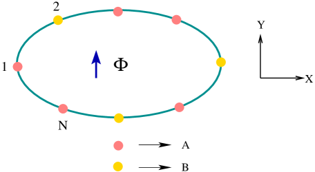
Figure 1: (Color online). Schematic diagram of a $5$th generation quasi-periodic Fibonacci mesoscopic ring subjected to Rashba and Dresselhaus spin-orbit interactions. The ring, composed of two different types of atomic sites A and B those are represented by two distinct colored filled circles, carries a net circulating charge current in presence of magnetic flux $\phi$.

to Rashba and Dresselhaus SO couplings. Two primary lattices, viz, $A$ and $B$ are used to get a $N$-site Fibonacci chain following the generation rule $F_{m}$ ($m\geq 3$) $=\left\{F_{m-1},F_{m-2}\right\}$ with $F_{1}=A$ and $F_{2}=AB$, which is then bent and coupled at its two ends to form a ring. Alternatively, we can think that $m$th generation Fibonacci sequence $F_{m}$ can be constructed using two lattice sites $A$ and $B$ applying $m$ times the inflation rules $A\rightarrow AB$ and $B\rightarrow A$ recursively, starting with the lattice $A$ or $B$. Here we start with the lattice $A$, for the sake of simplicity, and thus, $A$, $AB$, $ABA$, $ABAAB$, $ABAABABA$, $\dots$, etc., are the first few generations of the Fibonacci sequence. Therefore, as an example, $F_{4}=ABAAB$ forms a $5$-site ($N=5$) Fibonacci ring. This is one representation, the so-called site model fib2 ; fib4 , of a Fibonacci generation. Another form of it is also conveniently used which is known as bond model bond1 ; bond2 where long ($L$) and short ($S$) bonds are taken into account, setting identical lattice sites. In few cases mixed model fib4 , a combination of site and bond models, is also used in studying electronic behavior. For the sake of simplicity here we restrict ourselves to the first configuration.

Based on a tight-binding (TB) framework we compute persistent current using second-quantized approach san2 . With this formalism one can find current carried by individual energy levels, and, from that total current for a particular band filling can be easily estimated. The major advantage of this technique is that, it reduces numerical errors especially for larger rings by avoiding the derivative of ground state energy with respect to flux $\phi$, as used in conventional current calculations gefen ; spl ; san3 . Most importantly, studying individual state currents conducting nature of different eigenstates can be determined which is quite significant to understand the response of a complete system. Thus, utilizing it, the crucial role played by SO interactions on current carrying states can be analyzed clearly, which is one key motivation behind this work. We find that state currents get increased significantly with SO coupling, which thus provide a large net current and sometimes it becomes orders of magnitude higher than the SOI-free Fibonacci rings. Undoubtedly this is an important observation and might throw some light in the era of deep-rooted debate between the experimental observations and theoretical estimates of current amplitudes.

Apart from this, we also discuss the behavior of persistent current for different band fillings, and, on its won merit, the quasi-periodic structure exhibits several anomalous features which can have great signature, particularly, in the aspect of controlling conducting nature of the full system.

Finally, we make a detailed analysis to find a scaling relation of persistent current with ring size $N$, associated with the generation $F_{m}$. From our extensive numerical analysis we establish that for a typical flux $\phi$, the current obeys a relation $CN^{-\xi}$, where $\xi$ depends on the ratio between the site energy difference and nearest-neighbor hopping integral. Thus keeping the ratio constant, site energies as well as hopping integral can be tuned and with these changes $\xi$ remains invariant. The pre-factor $C$ strongly depends on both SO coupling and magnetic flux, which is also reported here in detail for the completeness. These results offer a unique opportunity to determine persistent current in a Fibonacci ring, subjected to SO coupling, for any arbitrary flux $\phi$ without doing any numerical simulation. This is another essential motivation for the present investigation.

We organize the rest of the article as follows. In Sec. II we present the model and its Hamiltonian in tight-binding framework. The procedure for calculating persistent current carried by different eigenstates as well as the net current for a particular electron filling is given in Sec. III, and the numerical results are discussed in Sec. IV. Finally, in Sec. V we summarize our main results.

II Model and Tight-binding Hamiltonian

We start by referring to Fig. 1, where a quasi-periodic mesoscopic Fibonacci ring composed of two different types of atomic sites $A$ and $B$ is given. The ring, subjected to both Rashba and Dresselhaus SO interactions, carries a net circulating charge current in presence of an AB flux $\phi$.

To illustrate this model quantum system we adopt a tight-binding framework. In the absence of electron-electron interaction the TB Hamiltonian for a $N$-site Fibonacci ring can be described as following:

$$H=H_{\mbox{\tiny 0}}+H_{\mbox{\tiny rashba}}+H_{\mbox{\tiny dressl}}.$$ (1)

The first term, $H_{\mbox{\tiny 0}}$, represents the Fibonacci ring in the absence of SO interactions and it becomes

$$H_{\mbox{\tiny 0}}=\sum_{n}\mbox{\boldmath$c$}_{n}^{{\dagger}}\mbox{\boldmath$\epsilon$}\mbox{\boldmath$c$}_{n}+\sum_{n}\left(e^{i\theta}\mbox{\boldmath$c$}_{n+1}^{{\dagger}}\mbox{\boldmath$t$}\mbox{\boldmath$c$}_{n}+e^{-i\theta}\mbox{\boldmath$c$}_{n}^{{\dagger}}\mbox{\boldmath$t$}^{{\dagger}}\mbox{\boldmath$c$}_{n+1}\right)$$ (2)

where $\theta=2\pi\phi/N$ is the phase factor due to the flux $\phi$ which is measured in unit of the elementary flux quantum $\phi_{0}$ ($=ch/e$), and $n=1$, $2$, $3$ $\dots$. The other factors are described as follows.
$\mbox{\boldmath$c$}_{n}=\left(\begin{array}[]{c}c_{n\uparrow}\\ c_{n\downarrow}\end{array}\right)$ and $\mbox{\boldmath$c$}^{\dagger}_{n}=\left(\begin{array}[]{cc}c_{n\uparrow}^{\dagger}&c_{n\downarrow}^{\dagger}\end{array}\right)$, where $c_{n\sigma}^{\dagger}$ ($c_{n\sigma}$) is the creation (annihilation) operator for an electron at $n$-th site with spin $\sigma(\uparrow,\downarrow)$. Considering the on-site potential at $n$th site for an electron with spin $\sigma$ as $\epsilon_{n\sigma}$ we express $\mbox{\boldmath$\epsilon$}_{n}=\left(\begin{array}[]{cc}\epsilon_{n\uparrow}&0\\ 0&\epsilon_{n\downarrow}\end{array}\right)$. Depending on the atomic site $A$ or $B$, $\epsilon_{n\sigma}$ becomes $\epsilon_{n\sigma}^{A}$ or $\epsilon_{n\sigma}^{B}$. $t$ is ($2\times 2$) diagonal matrix with the diagonal elements $\mbox{\boldmath$t$}_{11}=\mbox{\boldmath$t$}_{22}=t$, where $t$ represents the nearest-neighbor hopping integral.

The second term, $H_{\mbox{\tiny rashba}}$, describes the Hamiltonian associated with Rashba SO coupling san2 and it becomes

$$H_{\mbox{\tiny rashba}} = -\sum_{n}\alpha\left[\mbox{\boldmath$c$}_{n+1}^{{\dagger}}\left(i\mbox{\boldmath$\sigma$}_{x}\cos\varphi_{n,n+1}+i\mbox{\boldmath$\sigma$}_{y}\sin\varphi_{n,n+1}\right)\right.$$ (3)

$$\left.e^{i\theta}\mbox{\boldmath$c$}_{n}+h.c.\right]$$

where $\alpha$ measures the Rashba SO coupling strength and $\varphi_{n,n+1}=\left(\varphi_{n}+\varphi_{n+1}\right)/2$ with $\varphi_{n}=2\pi(n-1)/N$. $\mbox{\boldmath$\sigma$}_{x}$ and $\mbox{\boldmath$\sigma$}_{y}$ are the Pauli spin matrices in $\mbox{\boldmath$\sigma$}_{z}$ diagonal representation.

In a quite similar way we can write the last term of the total Hamiltonian Eq. 1 which is related to Dresselhaus SO coupling san2 as,

$$H_{\mbox{\tiny dressl}} = \sum_{n}\beta\left[\mbox{\boldmath$c$}_{n+1}^{{\dagger}}\left(i\mbox{\boldmath$\sigma$}_{y}\cos\varphi_{n,n+1}+i\mbox{\boldmath$\sigma$}_{x}\sin\varphi_{n,n+1}\right)\right.$$ (4)

$$\left.e^{i\theta}\mbox{\boldmath$c$}_{n}+h.c.\right]$$

where $\beta$ is the Dresselhaus coefficient.

III Theoretical Formulation

In this section, we calculate persistent charge current carried by individual eigenstates using the second-quantized approach and from these individual state currents we determine the net current for a particular electron filling.

We start with the current operator $\mbox{\boldmath$I$}=e\mbox{\boldmath$\dot{x}$}/(Na)$, where $a$ is the lattice spacing and $\dot{x}$ is the velocity operator written in the form,

$$\mbox{\boldmath$\dot{x}$}=\frac{1}{i\hbar}\left[\mbox{\boldmath$x$},\mbox{\boldmath$H$}\right]$$ (5)

where $\mbox{\boldmath$x$}=a\sum\limits_{n}\mbox{\boldmath$c$}_{n}^{\dagger}n\mbox{\boldmath$c$}_{n}$ denotes the position operator. Thus we can write the current operator as

$$\mbox{\boldmath$I$}=\frac{e}{Na}\frac{1}{i\hbar}\left[\mbox{\boldmath$x$},\mbox{\boldmath$H$}\right]=\frac{2\pi ie}{Nah}\left[\mbox{\boldmath$H$},\mbox{\boldmath$x$}\right].$$ (6)

Substituting $x$ and $H$ into Eq. 6 and doing quite lengthy but straightforward calculations we eventually reach to the expression

$$\mbox{\boldmath$I$}=\frac{2\pi ie}{Nh}\sum\limits_{n}\left(\mbox{\boldmath$c$}_{n}^{\dagger}\mbox{\boldmath$t$}_{\varphi}^{\dagger n,n+1}\mbox{\boldmath$c$}_{n+1}e^{-i\theta}-\mbox{\boldmath$c$}_{n+1}^{\dagger}\mbox{\boldmath$t$}_{\varphi}^{n,n+1}\mbox{\boldmath$c$}_{n}e^{i\theta}\right)$$ (7)

where $\mbox{\boldmath$t$}_{\varphi}^{n,n+1}$ is a ($2\times 2$) matrix whose elements are as follows: $\mbox{\boldmath$t$}_{\varphi,11}^{n,n+1}=\mbox{\boldmath$t$}_{\varphi,22}^{n,n+1}=t$, $\mbox{\boldmath$t$}_{\varphi,12}^{n,n+1}=-i\alpha e^{-i\varphi_{n,n+1}}+\beta e^{i\varphi_{n,n+1}}$, $\mbox{\boldmath$t$}_{\varphi,21}^{n,n+1}=-i\alpha e^{i\varphi_{n,n+1}}-\beta e^{i\varphi_{n,n+1}}$. Once $I$ is established, the current carried by any energy eigenstate $|\psi_{m}\rangle$ (say) can be calculated by the relation

$$I_{m}=\langle\psi_{m}|\mbox{\boldmath$I$}|\psi_{m}\rangle$$ (8)

where $|\psi_{m}\rangle=\sum\limits_{n}\left(a_{n\uparrow}^{m}|n\uparrow\rangle+a_{n\downarrow}^{m}|n\downarrow\rangle\right)$. $|n\sigma\rangle$’s are the Wannier states and $a_{n\sigma}^{m}$’s are the coefficients. After simplification we reach to the following

$$I_{m} = \frac{2\pi ie}{Nh}\sum\limits_{n}\left(ta_{n,\uparrow}^{m\ast}a_{n+1,\uparrow}^{m}e^{-i\theta}-ta_{n+1,\uparrow}^{m\ast}a_{n,\uparrow}^{m}e^{i\theta}\right)$$ (9)

$$+\frac{2\pi ie}{Nh}\sum\limits_{n}\left(ta_{n,\downarrow}^{m\ast}a_{n+1,\downarrow}^{m}e^{-i\theta}-ta_{n+1,\downarrow}^{m\ast}a_{n,\downarrow}^{m}e^{i\theta}\right)$$

$$+\frac{2\pi ie}{Nh}\sum\limits_{n}\left\{\left(i\alpha e^{-i\phi_{n,n+1}}+\beta e^{i\phi_{n,n+1}}\right)\times\right.$$

$$\left.a_{n,\uparrow}^{m\ast}a_{n+1,\downarrow}^{m}e^{-i\theta}\right.$$

$$+\left.\left(i\alpha e^{i\phi_{n,n+1}}+\beta e^{-i\phi_{n,n+1}}\right)a_{n+1,\downarrow}^{m\ast}a_{n,\uparrow}^{m}e^{i\theta}\right\}$$

$$+\frac{2\pi ie}{Nh}\sum\limits_{n}\left\{\left(i\alpha e^{i\phi_{n,n+1}}+\beta e^{-i\phi_{n,n+1}}\right)\times\right.$$

$$\left.a_{n,\downarrow}^{m\ast}a_{n+1,\uparrow}^{m}e^{-i\theta}\right.$$

$$+\left.\left(i\alpha e^{-i\phi_{n,n+1}}-\beta e^{i\phi_{n,n+1}}\right)a_{n+1,\uparrow}^{m\ast}a_{n,\downarrow}^{m}e^{i\theta}\right\}$$

This is the general expression of persistent charge current carried by an eigenstate $|\psi_{m}\rangle$ in presence of Rashba and Dresselhaus SO interactions. With this relation total charge current at absolute zero temperature ($T=0\,$K) for a $N_{e}$-electron system becomes

$$I=\sum\limits_{m=1}^{N_{e}}I_{m}$$ (10)

where the contributions from the lowest $N_{e}$ states are taken into account.

This is one way (viz, the second-quantized approach) of calculating persistent charge current which we use in this work due its potentiality for our present analysis. But, there exists another method, the so-called derivative method gefen ; spl , where net circulating current is evaluated by taking a first order derivative of ground state energy $E_{0}$ (say) with respect to AB flux $\phi$.

IV Numerical Results and Discussion

According to the theoretical formulation introduced in Sec. III we are now ready to analyze numerical results, computed in the limit of zero temperature, for charge current carried by individual energy levels, net current for a particular electron filling and its scaling behavior with system size in presence of Rashba and Dresselhaus SO interactions. In our model since the sites are non-magnetic we can write $\epsilon_{n\sigma}^{A}$ simply as $\epsilon_{A}$ for all $A$-type atomic sites, and similarly, for $B$-type sites $\epsilon_{n\sigma}^{B}=\epsilon_{B}$. When $\epsilon_{A}=\epsilon_{B}$, the system becomes a perfect ring as on-site energies are independent of site index $n$, and thus, we can set them to zero without loss of any generality. All the energies used in our calculations are scaled with respect to the nearest-neighbor hopping integral $t$ which is fixed at $1\,$eV throughout the presentation, and, we measure the current in unit of $et/h$.

Before addressing the central results of persistent current, let us have a look at the energy band spectrum for both perfectly ordered and Fibonacci rings to make the present work a self contained one.

IV.1 Energy Spectrum

In Figs. 2 and 3 flux dependent energy spectra are shown for a $8$-site perfectly ordered (viz, $\epsilon_{A}=\epsilon_{B}=0$) and Fibonacci ($\epsilon_{A}=-\epsilon_{B}=1\;$eV) rings, respectively. From the spectra it is clearly observed that the correlated disorder removes the energy level crossings noticed in the perfect case and also it reduces the slope of the energy levels. Most importantly we see that the number of energy levels gets twice when the ring is subjected to both AB flux $\phi$ and SO interaction compared to the SOI-free ring. From the fundamental principle of quantum mechanics it is well known that if the Hamiltonian is symmetric under time-reversal operation the Kramer’s degeneracy gets preserved, resulting degenerate energy levels. For our model, the two physical parameters, magnetic flux and SO coupling, affect the degeneracy.

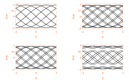
Figure 2: (Color online). Electronic energy levels of a $8$-site ring ($5$th generation) with $\epsilon_{A}=\epsilon_{B}=0$ as a function of flux $\phi$ for different values of $\alpha$ and $\beta$, where (a) $\alpha=\beta=0$; (b) $\alpha=1\;$eV, $\beta=0$; (c) $\alpha=0$, $\beta=1\;$eV and (d) $\alpha=0.5\;$eV, $\beta=1.5\;$eV.

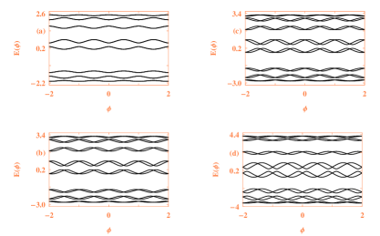
Figure 3: (Color online). Electronic energy levels of a $8$-site ring ($5$th generation) with $\epsilon_{A}=-\epsilon_{B}=1\;$eV as a function of flux $\phi$ for different values of $\alpha$ and $\beta$, where (a), (b), (c) and (d) correspond to the identical meaning as given in Fig. 2.

In presence of $\phi$ two-fold degenerate energy levels are obtained from the SOI-free (viz, $\alpha=\beta=0$) ring. Similar kind of two-fold degenerate energy states are also noted under time-reversal symmetry condition (i.e., $\phi=0$) when the ring is subjected to SO coupling. For this situation we can write $E(k,\uparrow)=E(-k,\downarrow)$ following the Kramer’s degeneracy, where $k$ represents the wave vector. But, it disappears completely as long as the magnetic flux is introduced ($E(k+\phi,\uparrow)\neq E(-k+\phi,\downarrow)$), and therefore, we get twice distinct energy levels compared to the SOI-free AB ring.

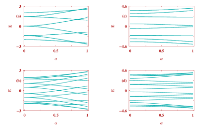
Figure 4: (Color online). Electronic energy levels as a function of Rashba SO coupling $\alpha$ of a $8$-site ring ($5$th generation) with $\epsilon_{A}=\epsilon_{B}=0$ for different values of $\phi$ and $\beta$, where (a) $\phi=\beta=0$; (b) $\phi=0.3$, $\beta=0$; (c) $\phi=0$, $\beta=1.5\;$eV and (d) $\phi=0.3$, $\beta=1.5\;$eV.

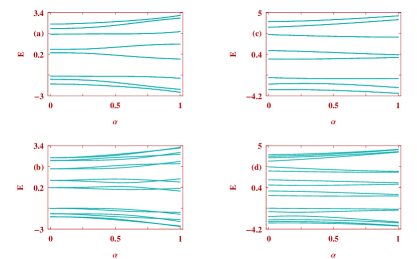
Figure 5: (Color online). Electronic energy levels as a function of Rashba SO coupling $\alpha$ of a $8$-site ring ($5$th generation) with $\epsilon_{A}=-\epsilon_{B}=1\;$eV for different values of $\phi$ and $\beta$, where (a), (b), (c) and (d) correspond to the identical meaning as given in Fig. 4.

In addition it is also crucial to note that even for perfectly ordered ring finite gaps appear near the two edges of the energy band spectrum when both the Rashba and Dresselhaus SO interactions are present (see Fig. 2(d)). The origin of such gaps in a ring system with $\alpha$ and $\beta$ has been described elaborately by Chang et al sheng in $2006$ and they have shown how the gap is sensitive with these parameter values.

In order to understand the precise role of SO coupling on energy levels in Figs. 4 and 5 we present the SO coupling dependent spectra for perfectly ordered and Fibonacci rings, respectively, considering the identical ring size as taken in Figs. 2 and 3, for different values of $\phi$ and $\beta$. With increasing the SO interaction strength splitting of the energy levels gets wider, while the degeneracy factors in different diagrams remains identical as discussed in the spectra Figs. 2 and 3. In these SOI dependent spectra (Figs. 4 and 5) eigenenergies are plotted as function of Rashba SO coupling setting some typical values of $\beta$. Exactly similar feature is also obtained under swapping the parameters $\alpha$ and $\beta$ (not shown here to save space), and its origin can be understood from the forthcoming sub-section.

IV.2 Enhancement of persistent current

Let us start with discussing the influence of SO couplings on the behavior of persistent current carried by individual energy eigenstates for a

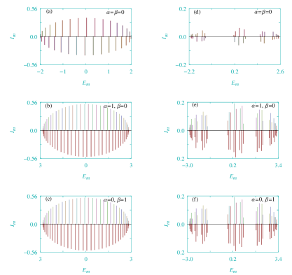
Figure 6: (Color online). Variation of persistent current $I_{m}$ carried by individual energy eigenstates $|\psi_{m}\rangle$ having eigenenergy $E_{m}$ of a $8$th generation Fibonacci ring at the typical flux $\phi=0.4$ for different values of Rashba and Dresselhaus SO interactions. In the left column we set $\epsilon_{A}=\epsilon_{B}=0$, while in the right column we choose $\epsilon_{A}=-\epsilon_{B}=1\;$eV.

typical flux $\phi$. The results of a $8$th generation Fibonacci ring are shown in Fig. 6 considering $\phi=0.4$, where the left column corresponds to $\epsilon_{A}=\epsilon_{B}=0$, while for the right column we choose $\epsilon_{A}=-\epsilon_{B}=1$. Several interesting features are obtained those are analyzed as follows.

At a first glance one can see that in the absence of SO coupling all distinct energy levels carry finite currents for the perfectly ordered ring

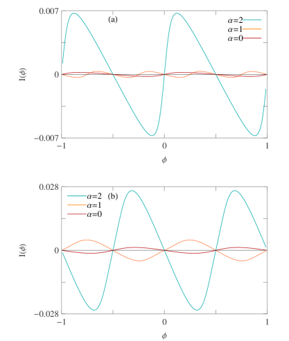
Figure 7: (Color online). Net current at a particular electron filling as a function of flux $\phi$ for some Fibonacci rings ($\epsilon_{A}=-\epsilon_{B}=1\;$eV) with different values of $\alpha$, where the red, orange and cyan curves correspond to $\alpha=0$, $1$ and $2\;$eV, respectively. The other physical parameters are: (a) $N=610$ ($14$th generation), $N_{e}=400$ and (b) $N=377$ ($13$th generation), $N_{e}=300$. Here we set $\beta=0$.

($\epsilon_{A}=\epsilon_{B}=0$), whereas these currents almost cease to zero in the case of correlated disordered ring ($\epsilon_{A}=-\epsilon_{B}=1\;$eV). This is quite obvious since a pure ring provides extended states which carry finite currents, while almost localized states obtained from the Fibonacci ring yield vanishingly small currents. These currents even more decrease with increasing the correlation strength ($|\epsilon_{A}\sim\epsilon_{B}|$) (which are not shown here in the figure). This fact has already been discussed in literature in connection with the localization aspects of different aperiodic crystal classes. But one of the major issues of our present investigation i.e., the interplay between SO interactions and quasiperiodic Fibonacci sequence on electronic localization has not been addressed earlier. To illustrate it, in the middle and last rows of Fig. 6 we show the dependence of state currents on $\alpha$ and $\beta$, respectively. A large number of discrete states of the Fibonacci ring, those were almost localized in absence of SO coupling (Fig. 6(d)), provides sufficiently large current in presence of non-zero SO coupling. This enhancement of current in presence of SO coupling can be elucidated in terms of quantum interference as it is directly related to the localization process. In presence of disorder, quantum interference gets dominated which gives rise to the electronic localized states, while this effect becomes weakened as a results of SO coupling as it involves spin-flipping, resulting enhanced charge currents. Naturally, this effect will be reflected into the net current for a particular band filling as discussed later. In addition, it is important to

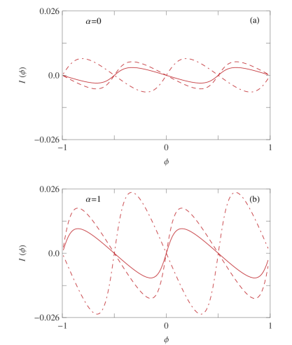
Figure 8: (Color online). Filling dependent current-flux characteristics of a $11$th generation Fibonacci ring ($\epsilon_{A}=-\epsilon_{B}=1\;$eV) where (a) $\alpha=0$ and (b) $\alpha=1\;$eV. The solid, dashed and dot-dashed curves correspond to $N_{e}=18$, $34$, and $56$, respectively. The Dresselhaus SO coupling is fixed at zero.

note that though the perfect ring exhibits extended states, they even carry higher currents in presence of finite SO coupling which is clearly spotted from the spectra given in the left column of Fig. 6.

Figure 6 also depicts that the nature (viz, magnitude and phase) of current carrying states remain unchanged under swapping the parameters $\alpha$ and $\beta$. This invariant nature can be understood through a simple mathematical argument. Inspecting carefully the Rashba and Dresselhaus Hamiltonians one can see that they are connected by a unitary transformation $U^{\dagger}H_{\mbox{\tiny rashba}}U=H_{\mbox{\tiny dressl}}$, where $U=(\mbox{\boldmath$\sigma$}_{x}+\mbox{\boldmath$\sigma$}_{y})/\sqrt{2}$ is the unitary matrix. Therefore, any eigenstate $|\psi_{p}\rangle$ (say) of the Rashba ring can be written in terms of the eigenstate $|\psi_{p}^{\prime}\rangle$ of the Dresselhaus ring where $|\psi_{p}\rangle=U|\psi_{p}^{\prime}\rangle$. This immediately gives the current for the Dresselhaus ring: $I_{p}(\mbox{for}~{}H_{\mbox{\tiny dressl}})=\langle\psi_{p}^{\prime}|\mbox{\boldmath$I$}|\psi_{p}^{\prime}\rangle=\langle\psi_{p}|U^{\dagger}\mbox{\boldmath$I$}U|\psi_{p}\rangle=\langle\psi_{p}|\mbox{\boldmath$I$}|\psi_{p}\rangle=I_{p}(\mbox{for}~{}H_{\mbox{\tiny rashba}})$. Hence, it is clearly observed that the nature of the current carrying states for the Rashba ring is exactly identical to that of the Dresselhaus ring. Using $SU(2)$ spin rotation transformation mechanism Sheng and Chang sheng have established that the Hamiltonian of the Rashba SOI alone is mathematically equivalent to that of the Dresselhaus SOI alone, and thus, our findings regarding the invariant nature of current carrying states under swapping the SOIs are consistent with their analysis.

Following the above characteristics of different current carrying states now we discuss the behavior of net current for a particular electron filling.

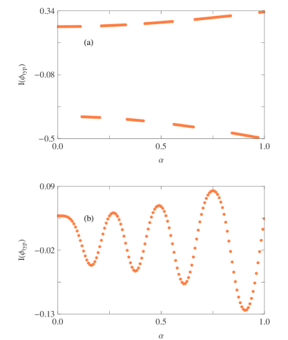
Figure 9: Current, evaluated at a particular flux $\phi=0.3\phi_{0}$, as a function of $\alpha$ ($\beta$ is fixed at zero) for (a) ordered and (b) Fibonacci ($\epsilon_{A}=-\epsilon_{B}=1\;$eV) rings considering $N=34$ ($8$th generation) and $N_{e}=20$.

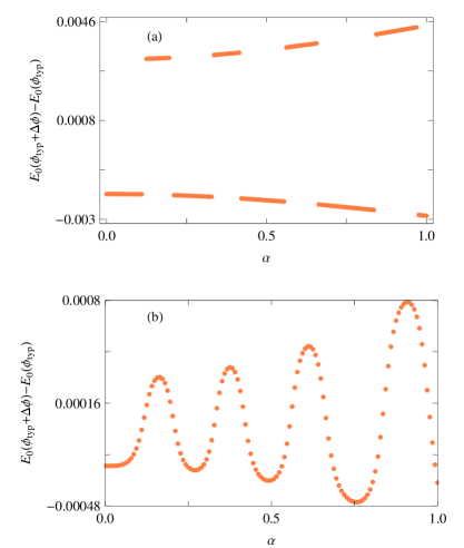
Figure 10: (Color online). Variation of $\Delta E_{0}$ with $\alpha$ at $\phi_{\mbox{\tiny typ}}=0.3\phi_{0}$ for the same parameter values as taken in Fig. 9, where (a) and (b) represent the identical meaning as given in Fig. 9. We choose $\Delta\phi=0.125/16$.

The results are shown in Fig. 7, where we show the variation of net persistent current as a function of $\phi$ for some typical Fibonacci rings considering different values of Rashba SO coupling. In (a) the currents are computed for $N=610$ ($14$th generation) and $N_{e}=400$, while in (b) these are performed for $N=377$ ($13$th generation) and $N_{e}=300$. From the spectra it is observed that the current almost vanishes for the entire flux window when the ring is free from SO coupling (red curves). This is solely due to the aperiodic nature of the site potentials. Introducing the SO coupling one can achieve higher current (orange lines), and, for a moderate SO coupling a dramatic change is observed (cyan curves), reflecting the $I_{m}$-$E_{m}$ spectra given in the right column of Fig. 6.

IV.3 Effect of electron filling

To test the dependence of persistent current on electron filling, in Fig. 8 we show the current-flux characteristics of a $11$th

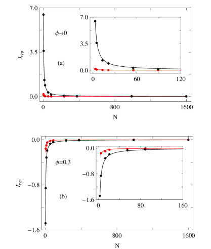
Figure 11: (Color online). Variation of current with ring size $N$ considering $\epsilon_{A}=-\epsilon_{B}=0.5\;$eV and $\beta=0$ where (a) $\phi\rightarrow 0$ and (b) $\phi=0.3$. The red and black dots, corresponding to $\alpha=0$ and $1.5\;$eV, respectively, are determined from the second-quantized approach. Using these dots we find scaling relation between $I_{\mbox{\tiny typ}}$ and $N$ which produces continuous curves depending on the scaling factors.

generation Fibonacci ring considering three different values of $N_{e}$. The results are shown for both zero (Fig. 8(a)) and finite (Fig. 8(b)) values of $\alpha$, where the solid, dashed and dot-dashed lines correspond to $N_{e}=18$, $34$ and $56$, respectively. For the ring without any SO coupling, currents are less fluctuating with $N_{e}$, while the fluctuation becomes significant in the presence of SO coupling. This is due to the irregular pattern of current amplitudes for different current carrying states (Fig. 6(e)). It is clearly observed from the spectrum Fig. 6(e) that one or more states those carry smaller currents reside among the higher current carrying states, and accordingly, when we set $N_{e}$ to a particular value, depending on the top most filled energy level higher or smaller current is obtained since the net current essentially depends on the contributions from the neighboring states of this highest filled level.

IV.4 Anomalous oscillation of current with SO coupling

The results analyzed so far are worked out only for some typical values of Rashba SO interaction. In order to establish the critical role played by SO interaction more precisely on persistent current now we focus on the

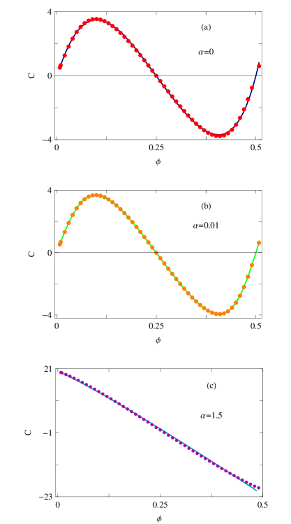
Figure 12: (Color online). Dependence of $C$ on $\phi$ at three distinct values of $\alpha$. The dotted points are evaluated by exactly calculating currents for a wide variation of ring size $N$ considering $\epsilon_{A}=-\epsilon_{B}=0.5\;$eV and $\beta=0$. Fitting these data sets we generate functional forms which provide continuous curves.

behavior given in Fig. 9, where we plot persistent current as a function of $\alpha$ for a particular flux $\phi=0.3\phi_{0}$. Both the perfect and Fibonacci rings reflect the fact that typical current gets increased with increasing $\alpha$ providing anomalous oscillations. Interestingly we see that in the impurity-free ring the typical current changes its sign alternately from positive to negative for a wide window of $\alpha$ and the window widths get broadened (Fig. 9(a)) for higher values of $\alpha$. On the other hand, a continuous variation with smaller current (Fig. 9(b)) is obtained in the Fibonacci ring. These features can be substantiated from the spectra shown in Fig. 10. Here we plot the difference $\Delta E_{0}$ of ground state energies, determined at two typical fluxes ($\phi_{\mbox{\tiny typ}}$, $\phi_{\mbox{\tiny typ}}+\Delta\phi$ ($\Delta\phi\rightarrow 0$)), as a function of $\alpha$ considering the same parameter values as taken in Fig. 9. The factor $-\Delta E_{0}/\Delta\phi$ gives the persistent current at $\phi_{\mbox{\tiny typ}}$, as used in conventional method, and thus from the nature of $\Delta E_{0}$-$\alpha$ characteristics (Fig. 10) we can estimate the oscillating behavior of current with $\alpha$ as $\Delta\phi$ is always positive. This is exactly what we present in Fig. 9.

IV.5 Scaling behavior

Finally, in this sub-section, we discuss size-dependent persistent current in presence of SO interaction and from that we try to find the scaling behavior.

Figure 11 demonstrates the variation of typical current $I_{\mbox{\tiny typ}}$ with system size $N$ for two different values of $\alpha$ in the half-filled limit. Two cases are analyzed depending on

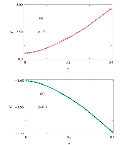
Figure 13: (Color online). Dependence of $C$ on $\alpha$ for two different values of $\phi$. The colored dots and the continuous lines correspond to the similar meaning as given in Fig. 12. The other parameters are: $\epsilon_{A}=-\epsilon_{B}=0.5\;$eV and $\beta=0$.

the flux $\phi$, one is for $\phi\rightarrow 0$ while for the other we set $\phi=0.3$, and they are presented in (a) and (b), respectively. The dots in the spectra are computed from the second-quantized approach and they obey a scaling relation of the form: $I_{\mbox{\tiny typ}}=CN^{-\xi}$ where $\xi=1$ and $1.03$ for $\alpha=0$ and $1.5\;$eV, respectively, which we find from our extensive numerical analysis. The pre-factor $C$ depends on both $\alpha$ and $\phi$. In the limit $\phi\rightarrow 0$, $C$ becomes $0.504$ and $19.718$ for $\alpha=0$ and $1.5\;$eV, respectively, while these values are $-0.862$ and $-4.564$, respectively, for $\phi=0.3$. Using this scaling relation we generate the continuous curves, where the black and red lines correspond to $\alpha=1.5\;$eV and $0$, respectively. Clearly we see that the curved lines fit the dots very well, and thus, we can utilize this scaling relation to find charge current for any generation at these typical values of $\alpha$ and $\phi$.

In analyzing Fig. 11 two important aspects should be noted. Firstly, the reduction of current with ring size $N$. The reason behind this reduction can be easily understood in terms of the coherence of electronic wave function. For smaller rings wave function becomes coherent throughout the ring yielding larger current, while the phase coherence gets reduced with increasing $N$ providing lesser current. Secondly, the current amplitudes of different Fibonacci rings satisfy a specific scaling law. This scaling behavior essentially comes from the quasiperiodicity of the system. The quasiperiodicity notably affects, as well, the energy band spectra of a Fibonacci ring (not shown here to save space). For instance, total energy bandwidth $\Delta E$ ($=\sum_{n}|E_{n}(\phi=0)-E_{n}(\phi=\phi_{0}/2)|$, where $E_{n}$’s are the eigenvalues) sharply decreases with the Fibonacci generation $F_{m}$ and it satisfies a similar kind of scaling relation with $F_{m}$. This is exactly reflected in $I_{\mbox{\tiny typ}}$-$N$ characteristics. Similar type of scaling nature is also obtained in other different quasiperiodic systems those have been described elsewhere new1 ; new2 ; new3 .

Following this analysis one question naturally arises how the coefficient $C$ depends on $\alpha$ and $\phi$, so that charge current can be estimated

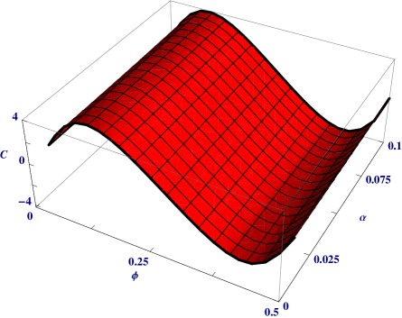
Figure 14: (Color online). Simultaneous variation of $C$ with $\alpha$ and $\phi$ for the Fibonacci rings described with $\epsilon_{A}=-\epsilon_{B}=0.5\;$eV and $\beta=0$.

at arbitrary values of these parameters for any generation of the quasi-periodic Fibonacci ring. The answer is given in Figs. 12-14.

Focusing on the spectra given in Fig. 12, we see that for lower values of $\alpha$, $C$-$\phi$ data exhibits sinusoidal-like pattern, though we cannot find a simple functional relationship with these data sets, and accordingly, here we do not present that functional form. On the other hand, for $\alpha=1.5\;$eV, $C$-$\phi$ data can be fitted well through a simple relation: $C=20.1-91\phi^{1.1}$ and it gives a linear-like variation with $\phi$ (Fig. 12(c)).

In Fig. 13 we demonstrate $C$-$\alpha$ characteristics for two typical values of flux $\phi$. Two different functional forms are obtained for these fluxes and they are: $C(\alpha)=0.57+17.72\alpha^{1.6}$ (for $\phi\rightarrow 0$) and $C(\alpha)=-1.68-2.25\alpha^{1.6}$ (for $\phi=0.3$).

At the same time, it is interesting as well as important to see the dependence of $C$ on both $\alpha$ and $\phi$ simultaneously. The result is given in Fig. 14 which clearly reflects the above scaling analysis as presented in Figs. 12-13.

For the complete analysis of scaling behavior now we discuss the interplay of Rashba and Dresselhaus SOIs on persistent current. The results are shown in Fig. 15 where the typical current is calculated for two different values of Rashba SO coupling, like Fig. 11, at two distinct AB fluxes ($\phi\rightarrow 0$ and $\phi=0.3$) considering the Dresselhaus SO coupling $\beta=0.5\;$eV. The same scaling relation, viz, $I_{\mbox{\tiny typ}}=CN^{-\xi}$ is obtained where $\xi$ becomes $1$ and $1.08$ for $\alpha=0$ and $1.5\;$eV, respectively. The pre-factor $C$ depends on both the SO couplings and

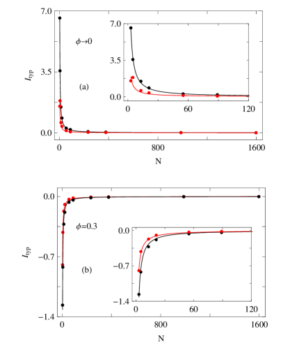
Figure 15: (Color online). Variation of current with ring size $N$ considering $\epsilon_{A}=-\epsilon_{B}=0.5\;$eV and $\beta=0.5\;$eV where (a) $\phi\rightarrow 0$ and (b) $\phi=0.3$. The colored dots and the continuous lines correspond to the similar meaning as described in Fig. 11.

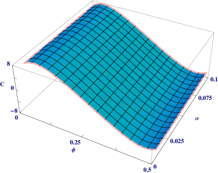
Figure 16: (Color online). Simultaneous variation of $C$ with $\alpha$ and $\phi$ for the Fibonacci rings described with $\epsilon_{A}=-\epsilon_{B}=0.5\;$eV and $\beta=0.5\;$eV.

flux $\phi$ as well. To have a complete idea about the variation of $C$ for a wide range of $\phi$ and $\alpha$ in presence of finite Dresselhaus SO coupling, in Fig. 16 we present a $3$D diagram (like Fig. 14), and, from this spectrum we can easily determine the pre-factor $C$ at the desired parameter values.

With these scaling results (Figs. 11-16) one can easily determine persistent current in any quasi-periodic Fibonacci ring in presence of SO couplings without doing detailed numerical calculations. Certainly this is a unique opportunity and has not been discussed before. $\bullet$ Application Perspective: All the results described above are worked out only for isolated rings. Now it is interesting and significant as well to know how such a system can be utilized in possible spintronic devices since SO interaction in low-dimensional geometries has attracted much attention due to its potential applications in diverse directions. For example, to enhance quantum information processing as well as quantum computation controlling electron’s spin degree of freedom is highly important dev1 . The SO interaction can provide much deeper insight for generating spin current and also its manipulation rather than conventional methodologies. Sometimes the interplay between Rashba and Dresselhaus SO interactions may give a significant change in electronic transport, as discussed by several groups dev2 ; dev3 . In order to reveal these facts the ring has to be connected with external electrodes, viz, source and drain. In presence of such electrodes one can study different aspects of spin-dependent transport like, spin currents, spin resoled conductances, spin polarization to name a few. One such work has been done Wang and Chang towards this direction dev4 . They have studied two-terminal spin-dependent transport through a 1D ring subjected to both Rashba and Dresselhaus SO couplings. The interplay between these two SOIs leads to a significant change in electronic transmission, localization of electrons and also spin polarization of the current. They have also shown how conductance is sensitive to the ring-electrode interface geometry, and these results certainly give a great impact in designing future spintronic devices. Several other works mlt1 ; mlt2 ; mlt3 ; mlt4 ; mlt5 have also been put forward along this direction to explore many interesting features of spin transport in a bridge setup. Before the end, we would like to state that since the study in open system (viz, source-ring-drain system) requires a complete separate theoretical approach, here in the present manuscript we do not go for this. We will analyze these aspects in our future work.

V Closing Remarks

In conclusion, we have investigated the critical roles played by Rashba and Dresselhaus SO couplings on persistent charge current in a quasi-periodic Fibonacci ring threaded by a magnetic flux $\phi$. Using a tight-binding framework we have computed individual state currents as well as net current for a particular band filling based on second-quantized approach. Analyzing state currents we can predict the conducting nature of individual energy levels, which on the other hand, provides an important tool in understanding the net response of a complete system. From the calculation of net current we have found that SO interaction can enhance the current significantly and sometimes it becomes orders of magnitude higher compared to the SOI-free Fibonacci ring. This observation might throw some light in the era of deep-rooted doubt between the experimental observations and theoretical predictions of persistent current.

In the rest of our work, we have essentially focused on the scaling behavior of persistent current with ring size $N$, associated with the Fibonacci generation, and established a unique way of determining persistent charge current without going through detailed numerical calculations. In the analysis of scaling properties we have restricted ourselves to the half-filled band limit considering odd electron filling. But, these scaling relations can be well applied to the even electron filling for the half-filled band case, expect the small rings (viz, $F_{5}$ and $F_{8}$) where the current deviates slightly from our fitting curve. Indeed, the establishment of scaling relation for any general electron filling and for any disordered ring, be it random or made of any kind of quasi-periodic lattices, will be highly interesting and important too. These issues will be available in our next work and it is the first step towards this direction.

Finally, it should be important to note that throughout the analysis we have presented the results only for the site model. But almost identical features are also obtained for the bond model and even for the mixed model, which we verify through our exhaustive numerical analysis, and accordingly, here we do not present those results.

References

- (1) M. Büttiker, Y. Imry, and R. Landauer, Phys. Lett. A 96, 365 (1983).
- (2) L. P. Lévy, G. Dolan, J. Dunsmuir, and H. Bouchiat, Phys. Rev. Lett. 64, 2074 (1990).
- (3) E. M. Q. Jariwala, P. Mohanty, M. B. Ketchen, and R. A. Webb, Phys. Rev. Lett. 86, 1594 (2001).
- (4) N. O. Birge, Science 326, 244 (2009).
- (5) V. Chandrasekhar, R. A. Webb, M. J. Brady, M. B. Ketchen, W. J. Gallagher, and A. Kleinsasser, Phys. Rev. Lett. 67, 3578 (1991).
- (6) H. Bluhm, N. C. Koshnick, J. A. Bert, M. E. Huber, and K. A. Moler, Phys. Rev. Lett. 102, 136802 (2009).
- (7) V. Ambegaokar and U. Eckern, Phys. Rev. Lett. 65, 381 (1990).
- (8) A. Schmid, Phys. Rev. Lett. 66, 80 (1991).
- (9) U. Eckern and A. Schmid, Europhys. Lett. 18, 457 (1992).
- (10) L. K. Castelano, G.-Q. Hai, B. Partoens, and F. M. Peeters, Phys. Rev. B 78, 195315 (2008).
- (11) J. Splettstoesser, M. Governale, and U. Zülicke, Phys. Rev. B 68, 165341 (2003).
- (12) G.-H. Ding and B. Dong, Phys. Rev. B 76, 125301 (2007).
- (13) H. F. Cheung, Y. Gefen, E. K. Reidel, and W. H. Shih, Phys. Rev. B 37, 6050 (1988).
- (14) R. A. Smith and V. Ambegaokar, Europhys. Lett. 20, 161 (1992).
- (15) H. Bouchiat and G. Montambaux, J. Phys. (Paris) 60, 2695 (1989).
- (16) E. Gambetti-Césare, D. Weinmann, R. A. Jalabert, and Ph. Brune, Europhys. Lett. 60, 120 (2002).
- (17) S. K. Maiti, M. Dey, S. Sil, A. Chakrabarti, and S. N. Karmakar, Europhys. Lett. 95, 57008 (2011).
- (18) Y. M. Liu, R. W. Peng, G. J. Jin, X. Q. Huang, M. Wang, A. Hu, and S. S. Jiang, J. Phys.: Condens. Matter 14, 7253 (2002).
- (19) X. F. Hu, R. W. Peng, L. S. Cao, X. Q. Huang, M. Wang, A. Hu, and S. S. Jiang, J. Appl. Phys. 97, 10B308 (2005).
- (20) R. Z. Qiu and W. J. Hsueh, Phys. Lett. A 378, 851 (2014).
- (21) G. J. Jin, Z. D. Wang, A. Hu, and S. S. Jiang, Phys. Rev. B 55, 9302 (1997).
- (22) Y. A. Bychkov and E. I. Rashba, JETP Lett. 39, 78 (1984).
- (23) G. Dresselhaus, Phys. Rev. 100, 580 (1955).
- (24) R. Winkler, Spin-orbit coupling effects in two-dimensional electron and hole Systems (Springer, Berlin, 2003).
- (25) J. S. Sheng and K. Chang, Phys. Rev. B 74, 235315 (2006).
- (26) L. Meier, G. Salis, I. Shorubalko, E. Gini, S. Schön, and K. Ensslin, Nature Physics 3, 650 (2007).
- (27) S. N. Karmakar, A. Chakrabarti, and R. K. Moitra, Phys. Rev. B 46, 3660 (1992).
- (28) R. K. Moitra, A. Chakrabarti, and S. N. Karmakar, Phys. Rev. B 66, 064212 (2002).
- (29) S. K. Maiti, J. Appl. Phys. 110, 064306 (2011).
- (30) S. K. Maiti, Solid State Commun. 150, 2212 (2010).
- (31) M. Kohmoto, Phys. Rev. Lett. 51, 1198 (1983).
- (32) P. Hawrylak and J. J. Quinn, Phys. Rev. Lett. 57, 380 (1986).
- (33) T. Janssen and M. Kohmoto, Phys. Rev. B 38, 5811 (1988).
- (34) S. A. Wolf, D. D. Awschalom, R. A. Buhrman, J. M. Daughton, S. von Molnár, M. L. Roukes, A. Y. Chtchelkanova, and D. M. Treger, Science 294, 1488 (2001).
- (35) M. C. Chang, Phys. Rev. B 71, 085315 (2005).
- (36) W. Yang and K. Chang, Phys. Rev. B 73, 045303 (2006).
- (37) M. Wang and K. Chang, Phys. Rev. B 77, 125330 (2008).
- (38) A. A. Kislev and K. W. Kim, J. App. Phys. 94, 4001 (2003).
- (39) I. A. Shelykh, N. G. Galkin, and N. T. Bagraev, Phys. Rev. B 72, 235316 (2005).
- (40) P. Földi, O. Kálmán, M. G. Benedict, and F. M. Peeters, Phys. Rev. B 73, 155325 (2006).
- (41) S. Souma and B. K. Nikolić, Phys. Rev. B 70, 195346 (2004).
- (42) S. K. Maiti, Phys. Lett. A 379, 361 (2015).