Randomized Alternating Least Squares for Canonical Tensor Decompositions: Application to A PDE With Random Data
Abstract.
This paper introduces a randomized variation of the alternating least squares (ALS) algorithm for rank reduction of canonical tensor formats. The aim is to address the potential numerical ill-conditioning of least squares matrices at each ALS iteration. The proposed algorithm, dubbed randomized ALS, mitigates large condition numbers via projections onto random tensors, a technique inspired by well-established randomized projection methods for solving overdetermined least squares problems in a matrix setting. A probabilistic bound on the condition numbers of the randomized ALS matrices is provided, demonstrating reductions relative to their standard counterparts. Additionally, results are provided that guarantee comparable accuracy of the randomized ALS solution at each iteration. The performance of the randomized algorithm is studied with three examples, including manufactured tensors and an elliptic PDE with random inputs. In particular, for the latter, tests illustrate not only improvements in condition numbers, but also improved accuracy of the iterative solver for the PDE solution represented in a canonical tensor format.
Key words and phrases:
Separated representations; Tensor Decomposition; Randomized Projection; Alternating Least Squares; Canonical Tensors; Stochastic PDE1. Introduction
The approximation of multivariate functions is an essential tool for numerous applications including computational chemistry [1, 24], data mining [2, 9, 24], and recently uncertainty quantification [11, 23]. For seemingly reasonable numbers of variables , e.g. , reconstructing a function, for instance, using its sampled values, requires computational costs that may be prohibitive. This is related to the so-called “curse of dimensionality.” To mitigate this phenomenon, we require such functions to have special structures that can be exploited by carefully crafted algorithms. One such structure is that the function of interest , depending on variables , admits a separated representation, [3, 4, 24], of the form
| (1.1) |
The number of terms, , is called the separation rank of and is assumed to be small. Any discretization of the univariate functions in (1.1) with , and , leads to a Canonical Tensor Decomposition, or CTD,
| (1.2) |
The functions in (1.1) and the corresponding vectors in (1.2) are normalized to unit norm so that the magnitude of the terms is carried by their positive -values, . It is well understood that when the separation rank is independent of , the computation costs and storage requirements of standard algebraic operations in separated representations scale linearly in , [4]. For this reason, such representations are widely used for approximating high-dimensional functions. To keep the computation of CTDs manageable, it is crucial to maintain as small as possible separation rank. Common operations involving CTDs, e.g. summations, lead to CTDs with separation ranks that may be larger than necessary. Therefore, a standard practice is to reduce the separation rank of a given CTD without sacrificing much accuracy, for which the workhorse algorithm is Alternating Least Squares (ALS) (see e.g., [3, 4, 6, 7, 21, 24, 31]). This algorithm optimizes the separated representation (in Frobenius norm) one direction at a time by solving least squares problems for each direction. The linear systems for each direction are obtained as normal equations by contracting over all tensor indices, , except those in the direction of optimization .
It is well known that forming normal equations increases the condition number of the least squares problem, see e.g. [16]. In this paper we investigate the behavior of the condition numbers of linear systems that arise in the ALS algorithm, and propose an alternative formulation in order to avoid potential ill-conditioning. As we shall see later, the normal equations in the ALS algorithm are formed via the Hadamard (entry-wise) product of matrices for individual directions. We show that in order for the resulting matrix to be ill-conditioned, the matrices for all directions have to be ill-conditioned and obtain estimates of these condition numbers. To improve the conditioning of the linear systems, we propose a randomized version of ALS, called randomized ALS, where instead of contracting a tensor with itself (in all directions but one), we contract it with a tensor composed of random entries. We show that this random projection improves the conditioning of the linear systems. However, its straightforward use does not insure monotonicity in error reduction, unlike in standard ALS. In order to restore monotonicity, we simply accept only random projections that do not increase the error.
Our interest here in using CTDs stems from the efficiency of such representations in tackling the issue of the curse of dimensionality arising from the solution of PDEs with random data, as studied in the context of Uncertainty Quantification (UQ). In the probabilistic framework, uncertainties are represented via a finite number of random variables specified using, for example, available experimental data or expert opinion. An important task is to then quantify the dependence of quantities of interest on these random inputs. For this purpose, approximation techniques based on separated representations have been recently studied in [12, 25, 26, 11, 27, 13, 18, 23, 10, 17, 19] and proven effective in reducing the issue of curse of dimensionality.
The paper is organized as follows. In Section 2, we introduce our notation and provide background information on tensors, the standard ALS algorithm, and the random matrix theory used in this paper. In Section 3, we introduce randomized ALS and provide analysis of the algorithm’s convergence and the conditioning of matrices used. Section 4 contains demonstrations of randomized ALS and comparisons with standard ALS on three examples. The most important of these examples provides background on uncertainty quantification and demonstrates the application of randomized ALS-based reduction as a step in finding the fixed point solution of a stochastic PDE. We conclude with a discussion on our new algorithm and future work in Section 5.
2. Notation and Background
2.1. Notation
Our notation for tensors, i.e. -directional arrays of numbers, is boldfaced uppercase letters, e.g. . These tensors are assumed to be in the CTD format,
where the factors are vectors with a subscript denoting the directional index and a superscript the rank index, and denotes the standard vector outer product. We write operators in dimension as , while for standard matrices we use uppercase letters, e.g. . Vectors are represented using boldfaced lowercase letters, e.g. , while scalars are represented by lowercase letters. We perform three operations on CTDs: addition, inner product, and the application of a -dimensional operator.
-
•
When two CTDs are added together, all terms are joined into a single list and simply re-indexed. In such a case the nominal separation rank is the sum of the ranks of the components, i.e., if CTDs are of the ranks and , the output has rank .
-
•
The inner product of two tensors in CTD format, and , is defined as
where the inner product operating on vectors is the standard vector dot product.
-
•
When applying a -dimensional operator to a tensor in CTD format, we have
We use the symbol to denote the standard spectral norm for matrices, as well as the Frobenius norm for tensors,
and and to denote the standard Euclidean and vector norms.
For analysis involving matrices we use three different types of multiplication in addition to the standard matrix multiplication. The Hadamard, or entry-wise, product of two matrices and is denoted by . The Kronecker product of two matrices and , is denoted as ,
The final type of matrix product we use, the Khatri-Rao product of two matrices and , is denoted by
We also frequently use the maximal and minimal (non-zero) singular values of a matrix, denoted as and , respectively.
2.2. ALS algorithm
Operations on tensors in CTD format lead to an increase of the nominal separation rank. This separation rank is not necessarily the smallest possible rank to represent the resulting tensor for a given accuracy. The ALS algorithm attempts to find an approximation to the tensor with minimal (or near minimal) separation rank. Specifically, given a tensor in CTD format with separation rank ,
and an acceptable error , we attempt to find a representation
with lower separation rank, , such that .
The standard ALS algorithm starts from an initial guess, , with a small separation rank, e.g., . A sequence of least squares problems in each direction is then constructed and solved to update the representation. Given a direction , we freeze the factors in all other directions to produce a least squares problem for the factors in direction . This process is then repeated for all directions . One cycle through all is called an ALS sweep. These ALS sweeps continue until the improvement in the residual either drops below a certain threshold or reaches the desired accuracy, i.e. . If the residual is still above the target accuracy , the separation rank is increased and we repeat the previous steps for constructing the representation with the new separation rank.
Specifically, as discussed in [4], the construction of the normal equations for direction can be thought of as taking the derivatives of the Frobenius norm of with respect to the factors , , and setting these derivatives to zero. This yields the normal equations
| (2.1) |
where corresponds to the -th entry of and is a vector indexed by . Alternatively, the normal system (2.1) can be obtained by contracting all directions except the optimization direction , so that the entries of the matrix are the Hadamard product of Gram matrices,
| (2.2) |
and, accordingly, the right-hand side is
We solve (2.1) for and use the solution to update . Pseudocode for the ALS algorithm is provided in Algorithm 1, where and denote the maximum separation rank and the limit on the number of iterations. The threshold is used to decide if the separation rank needs to be increased.
A potential pitfall of the ALS algorithm is poor-conditioning of the matrix since the construction of normal equations squares the condition number as is well known in matrix problems. An alternative that avoids the normal equations is mentioned in the review paper [24], but it is not feasible for problems with even moderately large dimension (e.g. ).
2.3. Estimate of condition numbers of least squares matrices
It is an empirical observation that the condition number of the matrices is sometimes significantly better than the condition numbers of some of the Gram matrices comprising the Hadamard product in (2.2). In fact we have
Lemma 1.
Let and be Gram matrices with all diagonal entries equal to . Then we have
If the matrix is positive definite, then
Since Gram matrices are symmetric non-negative definite, the proof of Lemma 1 follows directly from [22, Theorem 5.3.4]. This estimate implies that it is sufficient for only one of the matrices to be well conditioned to assure that the Hadamard product is also well conditioned. In other words, it is necessary for all directional Gram matrices to be ill-conditioned to cause the ill-conditioning of the Hadamard product. Clearly, this situation can occur and we address it in the paper.
2.4. Modification of normal equations: motivation for randomized methods
We motivate our approach by first considering an alternative to forming normal equations for ordinary matrices (excluding the QR factorization that can be easily used for matrices). Given a matrix , , we can multiply by a matrix with independent random entries and then solve
| (2.3) |
instead (see, e.g. [20, 29, 30, 33] ). The solution of this system, given that is of appropriate size (i.e., is large enough), will be close to the least squares solution [29, Lemma 2]. In [29], (2.3) is used to form a preconditioner and an initial guess for solving via a preconditioned conjugate gradient method. However, for our application we are interested in using equations of the form (2.3) in the Hadamard product in (2.2). We observe that typically has a smaller condition number than . To see why, recall that for full-rank, square matrices and , a bound on the condition number is
However, for rectangular full-rank matrices and , , this inequality does not necessarily hold. Instead, we have the inequality
| (2.4) |
where is the projection of onto the row space of (for a proof of this inequality, see Appendix A). If has a small condition number (for example, when is a Gaussian random matrix, see [8, 14, 15]) and we were to assume is close to , we obtain condition numbers smaller than . The assumption that is close to is the same as assuming the columns of lie within the subspace spanned by the row of . This is achieved by choosing to be larger than when is a randomized matrix.
2.5. Definitions and random matrix theory
The main advantage of our approach is an improved condition number for the linear system solved at every step of the ALS algorithm. We use a particular type of random matrices to derive bounds on the condition number: the rows are independently distributed random vectors, but the columns are not (instead of the standard case where all entries are i.i.d). Such matrices were studied extensively by Vershynin [32] and we rely heavily on this work for our estimates. To proceed, we need the following definitions from [32].
Remark 2.
Definitions involving random variables, and vectors composed of random variables, are not consistent with the notation of the rest of the paper, outlined in Section 2.1.
Definition 3.
[32, Definition 5.7] Let denote the probability of a set and the mathematical expectation operator. Also, let be a random variable that satisfies one of the three following equivalent properties,
where the constants , , differ from each other by at most an absolute constant factor (see [32, Lemma 5.5] for a proof of the equivalence of these properties). Then is called a sub-Gaussian random variable. The sub-Gaussian norm of is defined as the smallest in property 2, i.e.,
Examples of sub-Gaussian random variables include Gaussian and Bernoulli random variables. We also present definitions for sub-Gaussian random vectors and their norm.
Definition 4.
[32, Definition 5.7] A random vector is called a sub-Gaussian random vector if is a sub-Gaussian random variable for all . The sub-Gaussian norm of is subsequently defined as
where is the unit Euclidean sphere.
Definition 5.
[32, Definition 5.19] A random vector is called isotropic if its second moment matrix, , is equal to identity, i.e. . This definition is equivalent to
The following theorem from [32] provides bounds on the condition numbers of matrices whose rows are independent sub-Gaussian isotropic random variables.
Theorem 6.
[32, Theorem 5.38] Let be an matrix whose rows are independent, sub-Gaussian isotropic random vectors in . Then for every , with probability at least , one has
| (2.5) |
Here , , depend only on the sub-Gaussian norm
An outline of the proof of Theorem 6 will be useful for deriving our own results, so we provide a sketch in Appendix A. The following lemma is used to prove Theorem 6, and will also be useful later on in the paper. We later modify it to prove a version of Theorem 6 that works for sub-Gaussian, non-isotropic random vectors.
3. Randomized ALS algorithm
3.1. Alternating least squares algorithm using random matrices
We propose the following alternative to using the normal equations in ALS algorithms: instead of (2.2), define the entries of via randomized projections,
| (3.1) |
where is the -th column of a matrix , , with random entries corresponding to direction . The choice of is made to reduce the condition number of . As shown in Section 3.3, as the bound on goes to , where is the matrix for standard ALS, i.e. (2.2). In this paper we consider independent signed Bernoulli random variables, i.e., is either or each with probability . We have had some success using standard Gaussian random variables in our experiments as well. The proposed change also alters the right-hand side of the normal equations (2.1),
| (3.2) |
Equivalently, may be written as
Looking ahead, we choose random matrices such that is a tall, rectangular matrix. Solving the linear system (2.1) with rectangular will require a pseudo-inverse, computed via either the singular value decomposition (SVD) or a QR algorithm.
To further contrast the randomized ALS algorithm with the standard ALS algorithm, we highlight two differences: firstly, the randomized ALS trades the monotonic reduction of approximation error (a property of the standard ALS algorithm) for better conditioning. To adjust we use a simple tactic: if a randomized ALS sweep (over all directions) decreases the error, we keep the resulting approximation. Otherwise, we discard the sweep, generate independent random matrices , and rerun the sweep. Secondly, the randomized ALS algorithm can be more computationally expensive than the standard one. This is due to the rejection scheme outlined above and the fact that in the randomized algorithm has a larger number of rows than its standard counterpart, i.e., . Pseudocode of our new algorithm is presented in Algorithm 2.
Remark 8.
We have explored an alternative approach using projections onto random tensors, different from Algorithm 2. Instead of using in (3.1) to solve for , we use the QR factorization of to form a preconditioner matrix, similar to the approach of [29] for solving overdetermined least squares problems in a matrix setting. This preconditioner is used to improve the condition number of in (2.2). The approach is different from Algorithm 2: we solve the same equations as the standard ALS algorithm, but in a better conditioned manner. Solving the same equations preserves the monotone error reduction property of standard ALS. With Algorithm 2 the equations we solve are different, but, as shown in Section (3.2), the solutions of each least squares problem are close to the those obtained by the standard ALS algorithm.
We provide convergence results and theoretical bounds on the condition number of with entries (3.1) in Sections 3.2 and 3.3, respectively. Additionally, in Section 4, we empirically demonstrate the superior conditioning properties of defined in (3.1) relative to those given by the standard ALS in (2.2).
3.2. Convergence of the randomized ALS algorithm
Before deriving bounds on the condition number of (3.1), it is important to discuss the convergence properties of our algorithm. To do so for our tensor algorithm, we derive a convergence result similar to [33, Lemma 4.8]. In this analysis, we flatten our tensors into large matrices and use results from random matrix theory to show convergence. First, we construct the large matrices used in this section from (3.1). Writing the inner product as a sum allows us to group all the summations together,
We have
where we have expanded the product to get the sum of the products of individual entries. Introducing a multi-index , we define two matrices, and , where is large, i.e., we write
We note that these matrices can also be written as Khatri-Rao products,
| (3.3) |
Since is large, , both and are rectangular matrices. Similarly, we rewrite a vector in (3.2),
using the multi-index as
Using the introduced notation, and , we rewrite the normal equations (2.1) for direction and coordinate as
| (3.4) |
and the randomized version of those equations as
| (3.5) |
We highlight the notable difference between the random matrix above and those found in the usual matrix settings, for instance, in randomized least squares regression [20, 29, 30, 33]. Specifically, in the former, the entries of are not statistically independent and are products of random variables, whereas in the latter the entries are often i.i.d realizations of single random variables. In the present work, we utilize signed Bernoulli random variables, where the entries of are dependent but also follow a signed Bernoulli distribution. Whether there exists an optimal choice of distribution for setting the entries in the tensor case requires a careful examination which is beyond the scope of this paper.
Next, we present a convergence result showing that the solution to the least squares problem at each iteration of randomized ALS is close to the solution we would get using standard ALS. For ease of notation, we drop the subscript from and .
Lemma 9.
Given and where , and assuming that is the solution that minimizes 2 and is the solution that minimizes , then
| (3.6) |
where , , is a matrix with orthonormal columns from the QR factorization of the augmented matrix and where is assumed to have full rank.
Proof.
We form the augmented matrix and find its QR decomposition, , where , and , and has orthonormal columns. Therefore, we have
Using these decompositions of and , we define a matrix such that
and arrive at
assuming that is invertible. We address this additional assumption when discussing the bounds of the extreme singular values of in Theorem 12.
Starting from the left-hand side of (3.6), we have
Since multiplication by maps a vector to the column space of , there exists such that . Hence, we obtain
where in the last step we used the orthonormality of the columns of .
Next we estimate norms, and . First, we decompose using the singular value decomposition, . From the definition of the spectral norm we know . Using the SVD of and the definition of along with our assumption of invertibility of , we write
Hence , and the bound is
∎
We later use results from [32] to bound since is a random matrix whose rows are independent from one another, but whose columns are not. To use this machinery, specifically Theorem 6, we require the following lemma.
Lemma 10.
is a random matrix with isotropic rows.
Proof.
Using the second moment matrix, we show that the rows of are isotropic. Given a row of written in column form, , we form the second moment matrix,
and show
Hence and is isotropic.
From the Khatri-Rao product definition of the matrix (3.3), we write a column of as
Therefore, using properties of the Kronecker product (see, e.g. [24, equation (2.2)]) we can switch the order of the regular matrix product and the Kronecker products,
Taking the expectation and moving it inside the Kronecker product gives us
∎
Since is a tall rectangular matrix () with independent sub-Gaussian isotropic rows, we may use Theorem 5.39 from Vershynin to bound the extreme singular values.
Lemma 11.
For every , with probability at least we have
| (3.9) |
where and depend only on the sub-Gaussian norm of the rows of .
Proof.
Using Lemma 10 and Theorem 6, we have the following bound on the extreme condition numbers of for every , with probability at least ,
where and depend only on the sub-Gaussian norm of the rows of . Since , we have
with the same probability.
We now state the convergence result.∎
Theorem 12.
Given and where , and assuming that is the solution that minimizes 2 and is the solution that minimizes , then for every , with probability at least we have
where and depend only on the sub-Gaussian norm . The matrix , , is composed of orthonormal columns from the QR factorization of the augmented matrix and is assumed to have full rank.
3.3. Bounding the condition number of
To bound the condition number of , we use a modified version of Theorem 6. If the rows of were isotropic then we could use Theorem 6 directly. However, unlike in Lemma 10, this is not the case for . While the second moment matrix is not the identity, it does play a special role in the bound of the condition number since it is the matrix from the standard ALS algorithm. To see this, we take the th row of , , and form the second moment matrix of ,
Since is a vector composed of either Bernoulli or standard Gaussian random variables, . Therefore, we are left with
We need to modify Theorem 6 for matrices that have independent, non-isotropic rows. In [32, Remark 5.40] it is noted in the case of a random matrix with non-isotropic rows that we can apply Theorem 6 to instead of . The matrix has isotropic rows and, thus, we obtain the following inequality that holds with probability at least ,
| (3.10) |
and , .
To clarify how (3.10) changes the bounds on the singular values and of a matrix with non-isotropic rows, we modify Lemma 7.
Lemma 13.
Consider matrices and (non-singular) that satisfy
| (3.11) |
for . Then we have the following bounds on the extreme singular values of :
The proof of Lemma 13 is included in Appendix A. Using Lemma 13, we observe that the bound on the condition number of a matrix satisfying (3.11) has the following form:
Using Lemma 13, we prove an extension of Theorem 6 for matrices with non-isotropic rows.
Theorem 14.
Let be an matrix whose rows, , are independent, sub-Gaussian random vectors in . Then for every , with probability at least one has
Here , , depend only on the sub-Gaussian norm and the norm of .
Proof.
We form the second moment matrix using rows and apply Theorem (6) to the matrix , which has isotropic rows. Therefore, for every , with probability at least , we have
| (3.12) |
where , , depend only on the sub-Gaussian norm . Applying Lemma 13 to (3.12) with and , results in the bound
with the same probability as (3.12).
To move outside the sub-Gaussian norm, we bound from above using the sub-Gaussian norm of ,
hence . Using this inequality, we bound the probability in (6.4) for the case of Theorem 6 applied to .
The last step, similar to the proof of Theorem 6, comes from choosing large enough, for example ).
∎
The combination of Lemma 13, the fact that for (3.1) is the same matrix as (2.2) (denoted below as ), and Theorem 14, leads to our bound on the condition number of in (3.1) is, for every and with probability at least ,
| (3.13) |
where the definitions of and are the same as in Theorem 14.
Remark 15.
In both (3.9) and (3.13) the ratios and are present. As both ratios go to zero, our bound on the condition number of goes to , and the bound on the condition number of goes to . These properties explain our choice to set as a constant multiple of in the randomized ALS algorithm. As with similar bounds for randomized matrix algorithms, these bounds are pessimistic. Hence does not have to be very large with respect to in order to get acceptable results.
Another reason to choose as a constant multiple of is the construction of in (3.3) and our choice to use Bernoulli random numbers. If is too small, there is the danger of the matrix becoming singular due to the size of and repeated rows. Choosing the constant multiple that defines large enough helps mitigate this problem.
4. Examples
4.1. Sine function
Our first test of the randomized ALS algorithm is to reduce a CTD generated from samples of the multivariate function . This reduction problem was studied in [4], where the output of the standard ALS algorithm suggested a new trigonometric identity yielding a rank separated representation of . As input, we use standard trigonometric identities to produce a rank initial CTD.
We ran tests using both standard ALS and the new randomized algorithm to reduce the separation rank of a CTD of samples of . The tests differed in that each one had a different random initial guess with separation rank . In this example we chose and sampled each variable , , with equispaced samples in the interval . Our input CTD for both algorithms was rank and was generated via a standard trigonometric identity. The reduction tolerance for both algorithms was set to , and the maximum number of iterations per rank, i.e. in Algorithm 1 and Algorithm 2, was set to . For tests involving the standard ALS algorithm we used a stuck tolerance of . To test the randomized ALS algorithm we used matrices of size and set in Algorithm 2 to .
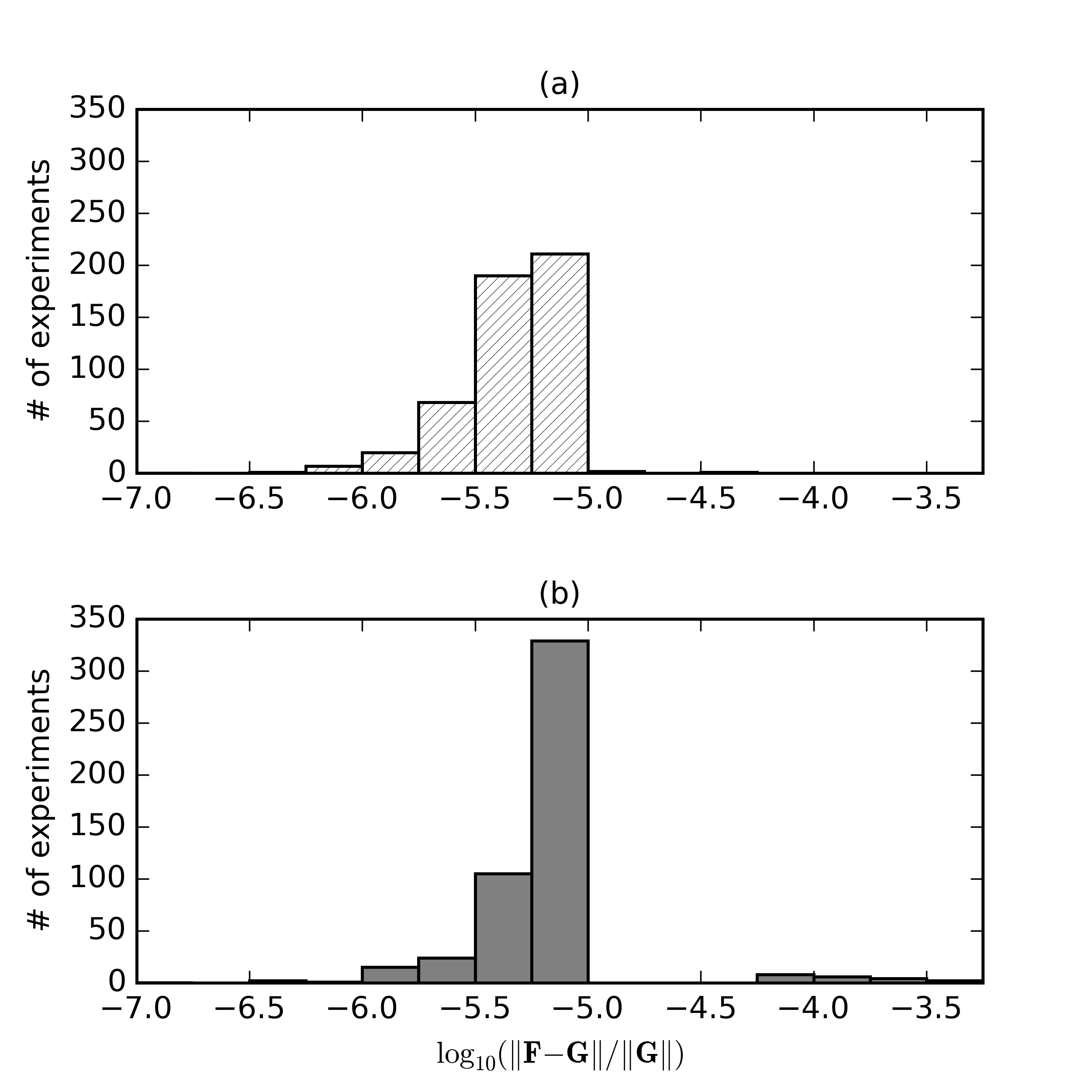
According to Lemma 2.4 in [4], there exists exact rank separated representations of . Using for our reduction tolerance, we were able to find rank approximations with both standard ALS and our randomized ALS whose relative errors were less than the requested (for a histogram of residuals of the tests, see Figure 4.1).
Due to the random initial guess and our choices of parameters (in particular the stuck tolerance and ) both algorithms had a small number of runs that did not find rank approximations with the requested tolerance . The randomized ALS algorithm produced fewer of these outcomes than standard ALS.
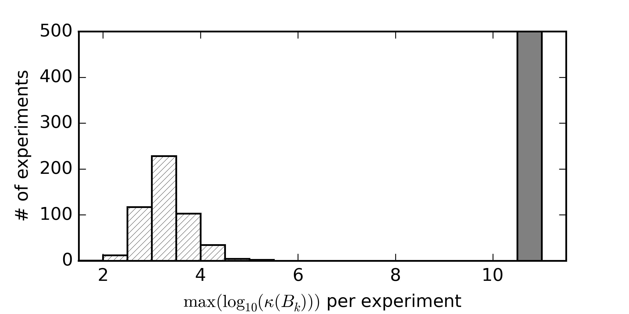
Large differences in maximum condition number (of ALS solves) are illustrated in Figure 4.2, where we compare tests of the standard and randomized ALS algorithms. We observe that the maximum condition numbers produced by the randomized ALS algorithm are much smaller those from the standard ALS algorithm. This is consistent with our theory.
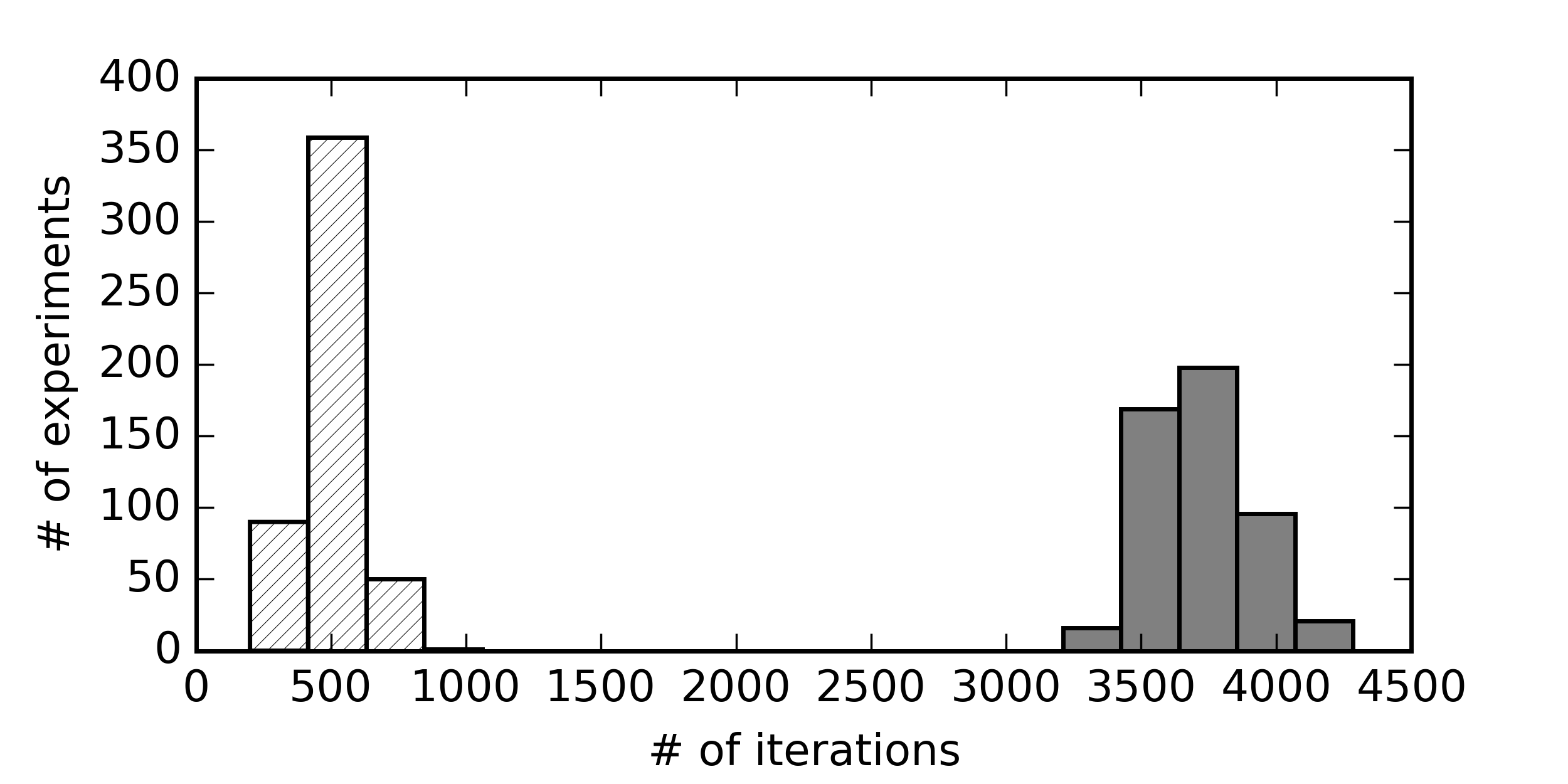
Furthermore, as shown in Figure 4.3, the number of iterations required for randomized ALS to converge was smaller than the number required by standard ALS. It is important to remember that the number of iterations required by the standard ALS algorithm to reduce a CTD can be optimized by adjusting the tolerance, stuck tolerance, and maximum number of iterations per rank. In these experiments we chose the stuck tolerance and maximum number of iterations to reduce the number of tests of the standard ALS algorithm that did not meet the requested tolerance .
4.2. A manufactured tensor
Our next test is to compare the performance of the standard and randomized ALS algorithms on a manufactured random tensor example. To construct this example we generate factors by drawing random samples from the standard Gaussian distribution. We chose and set the separation rank of the input tensor to . Then we normalized the factors and set the s-values of the tensor equal to , , where was predetermined such that is small.
Similar to the sine example, we ran experiments and requested an accuracy of from both algorithms. The maximum number of iterations for both algorithms was set to , while the stuck tolerance for the standard ALS algorithm was set to . We used the following parameters for the randomized ALS algorithm: the matrices were of size , and the repetition parameter, in Algorithm 2, was set to . We started all tests from randomized guesses with rank . This value was chosen because in all previous runs the reduced separation rank never fell below . Such an experiment allows us to compare how the algorithms perform when the initial approximation has rank greater than one.
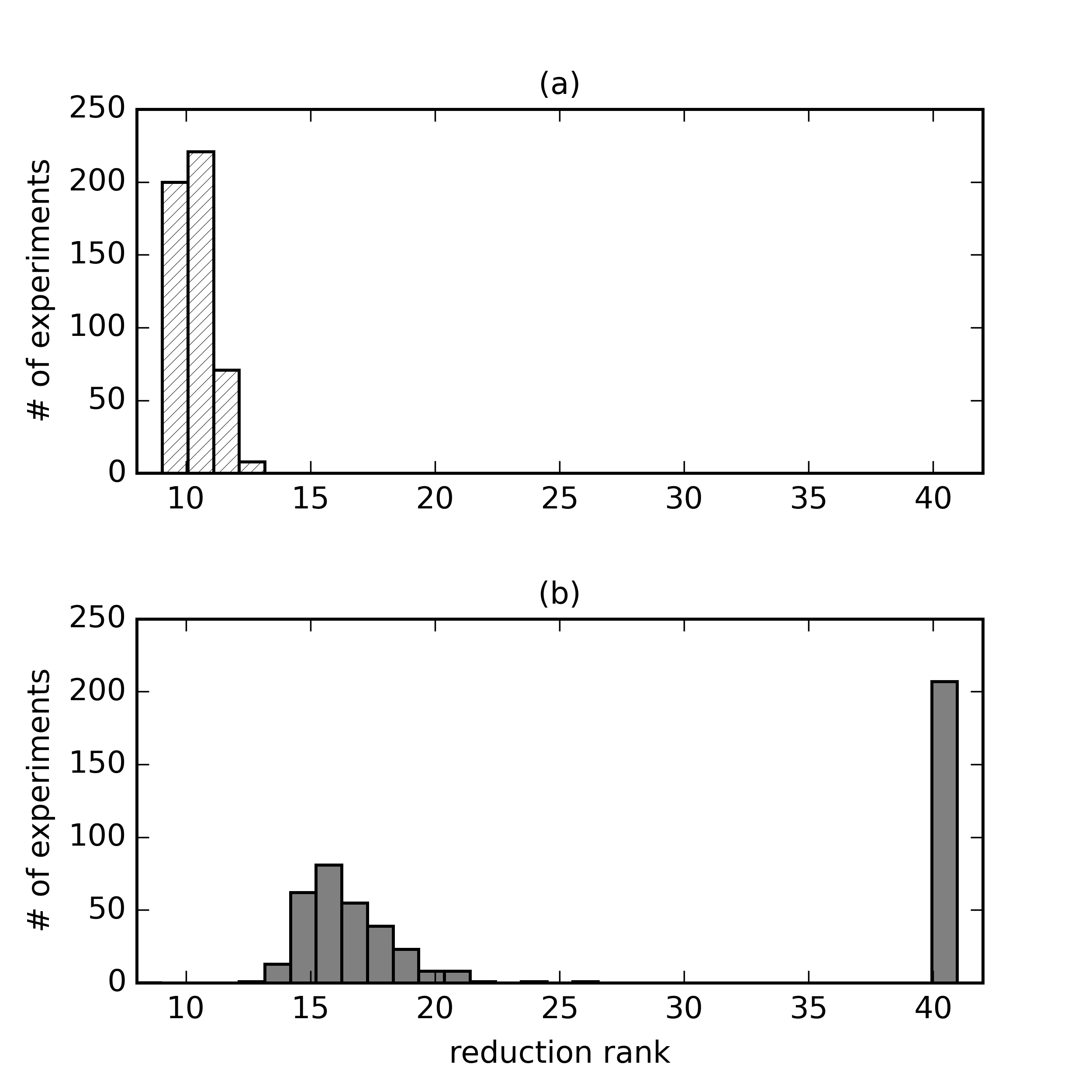
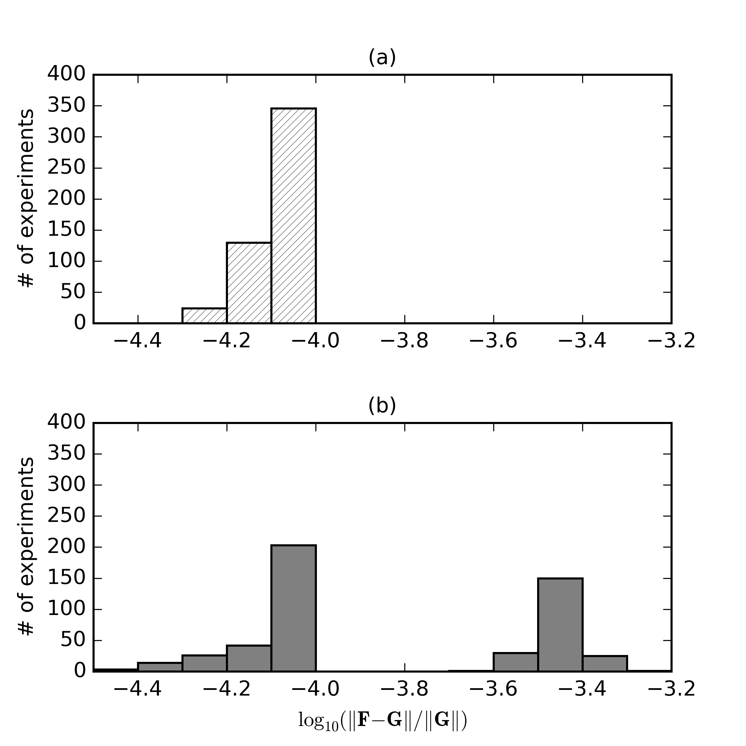
We show in Figure 4.4 the output separation ranks from tests of both the randomized and standard ALS algorithms. The CTD outputs from randomized ALS had, on average, lower separation ranks than those from standard ALS. Furthermore, as seen in Figure 4.4, some of the output CTDs from the standard ALS algorithm had separation rank above . In these instances, standard ALS failed to reduce the separation rank of the input CTD because simple truncation to would have given double precision. These failures did not occur with the randomized ALS algorithm. We can also see the contrast in performance in Figure 4.5: all tests of the randomized ALS algorithm produced CTDs with reduced separation rank whose relative reduction errors were less than the accuracy . Also, in Figure 4.5, we observe instances where the standard ALS algorithm failed to output a reduced separation rank CTD with relative error less than .
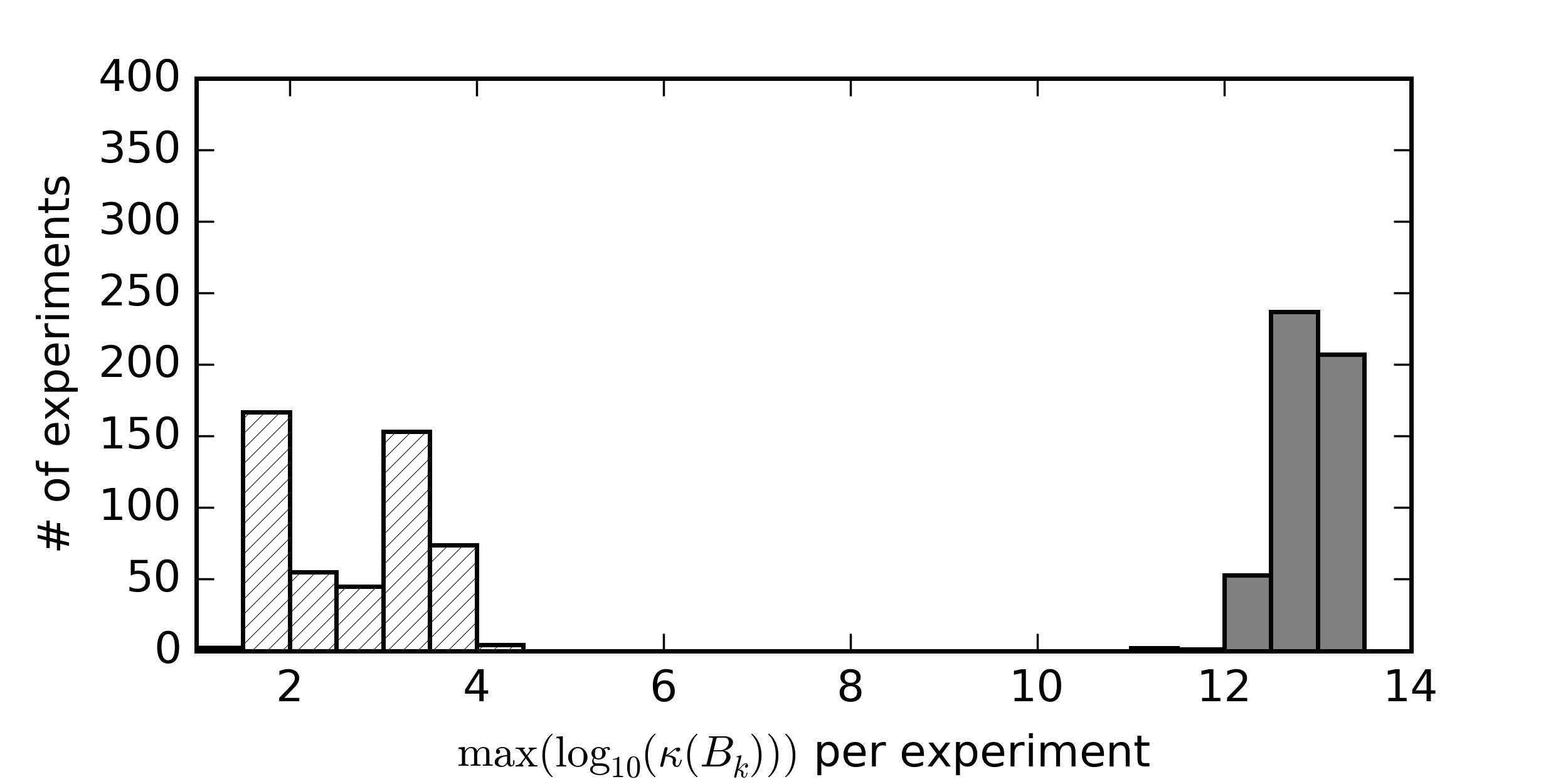
There was a significant difference in the maximum condition numbers of matrices used in the two algorithms. In Figure 4.6, we see that matrices produced by standard ALS had much larger condition numbers (by a factor of roughly ) than their counterparts in the randomized ALS algorithm. Such large condition numbers may explain the failures of the standard ALS algorithm to output reduced separation rank CTDs with relative errors less than .
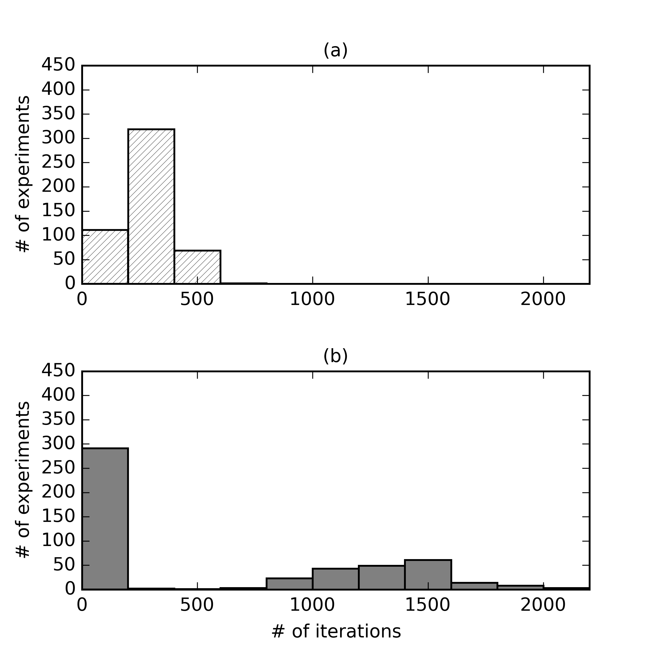
From Figure 4.7, we see that in many cases standard ALS required fewer iterations than the randomized ALS algorithm to converge. However, relative to randomized ALS, standard ALS required a large number of iterations for a considerable fraction of the experiments.
4.3. Elliptic PDE with random coefficient
As the key application of the randomized ALS algorithm, we consider the separated representation of the solution to the linear elliptic PDE
| (4.1) | |||||
defined on the unit square with boundary . The diffusion coefficient is considered random and is modeled by
| (4.2) |
where and the random variables are independent and uniformly distributed over the interval , and we choose , , and . In (4.2), are the largest eigenvalues associated with , the -orthonormalized eigenfunctions of the exponential covariance function
| (4.3) |
where denotes the correlation length, here set to . Given the choices of parameters , , , and , the model in (4.2) leads to strictly positive realizations of .
We discretize (4.1) in the spatial domain via triangular finite elements of size . This discretization, along with the affine representation of in , yields the random linear system of equations
| (4.4) |
for the approximate vector of nodal solutions . The sparse matrices and are obtained from the finite element discretization of the differential operator in (4.1) assuming is replaced by and , respectively.
To fully discretize (4.4), we consider the representation of at a tensor-product grid where, for each , the grid points are selected to be the Gauss-Legendre abscissas. In our numerical experiments, we used the same number of abscissas for all . The discrete representation of (4.4) is then given by the tensor system of equations
| (4.5) |
where the linear operation is defined as
and for ,
where
and is the identity matrix. The tensor in (4.5) is defined as
where is an -vector of ones. We seek to approximate in (4.5) with a CTD,
| (4.6) |
where the separation rank will be determined by a target accuracy. In (4.6) and , . To solve (4.5), we use a fixed point iteration similar to those used for solving matrix equations and recently employed to solve tensor equations in [23]. In detail, the iteration starts with an initial tensor of the form in (4.6). At each iteration , is updated according to
while requiring . To assure this requirement is satisfied we solve
| (4.7) |
where is chosen such that . We compute the operator norm via power method; see, e.g., [4, 5].
One aspect of applying such an iteration to a CTD is an increase in the output separation rank. For example, if we take a tensor of separation rank and use it as input for (4.7), one iteration would increase the rank to . Therefore we require a reduction algorithm to decrease the separation rank as we iterate. This is where either the standard or randomized ALS algorithm is required: to truncate the separated representation after we have run an iteration. Both ALS methods work with a user-supplied truncation accuracy , so we denote the reduction operator as . Including this operator into our iteration, we have
| (4.8) |
Pseudocode for our fixed point algorithm is shown in Algorithm 3
Remark 16.
In this example, the separation rank of is directly related to the problem dimension , i.e. , which is a consequence of using a Karhunen-Loeve-type expansion for finite-dimensional noise representation of . This will increase the computational cost of the algorithm to more than linear with respect to , e.g. quadratic in when an iterative solver is used and . Alternatively, one can obtain the finite-dimensional noise representation of by applying the separated rank reduction technique of this study on the stochastic differential operator itself to possibly achieve . The interested reader is referred to [3, 4] for more details.
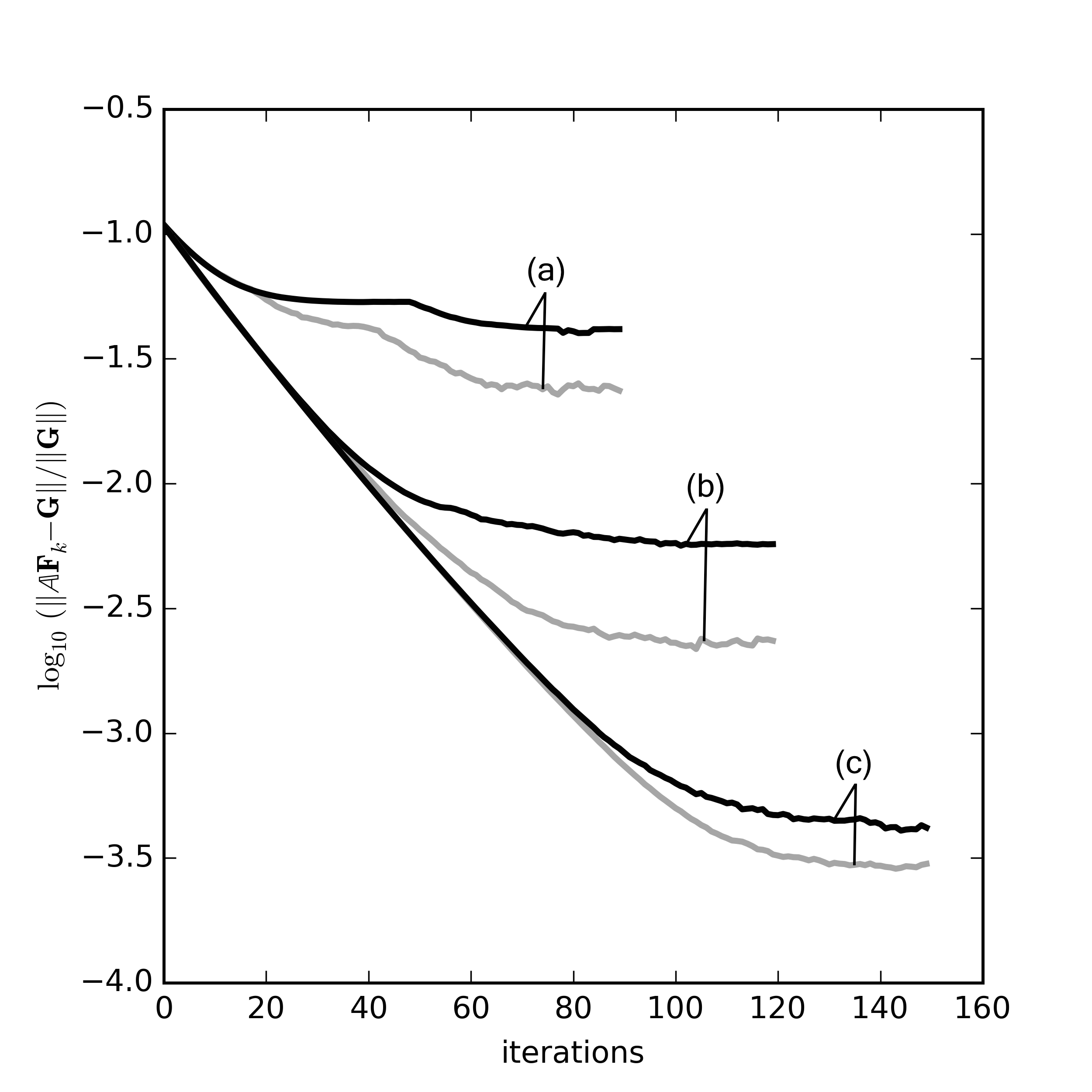
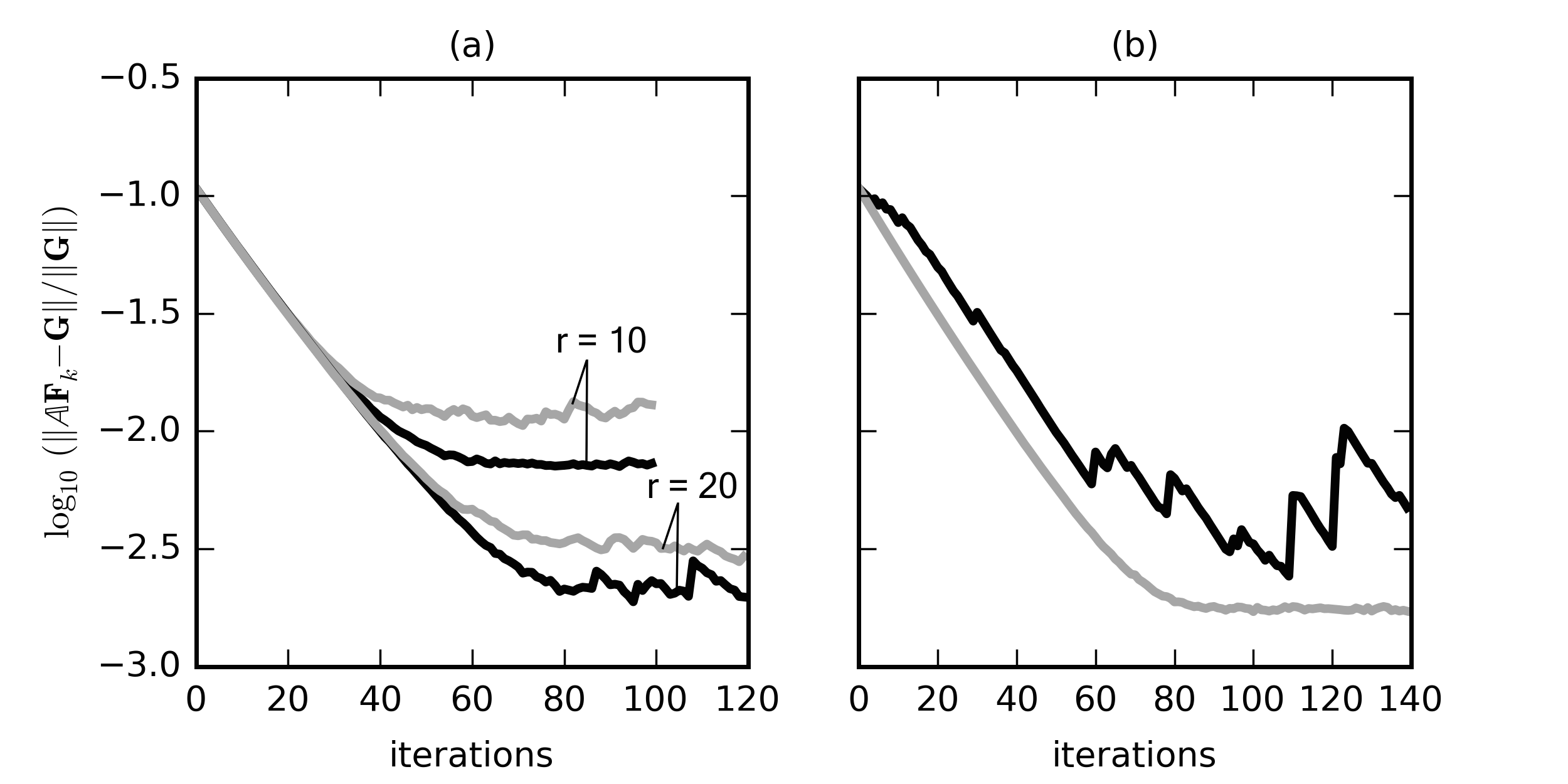
First, we examine the convergence of the iterative algorithm given a fixed ALS reduction tolerance in Figure 4.8. The randomized ALS method converges to more accurate solutions in all of these tests (see Table 1). However, the ranks of the randomized ALS solutions are larger than the ranks required for solutions produced by the standard ALS algorithm.
In Figure 4.9, we observe different behavior in the relative residuals using fixed ranks instead of fixed accuracies. For these experiments the ALS-based linear solve using the standard algorithm out-performs the randomized version, except in the rank case (see Table 2). In this case, the standard ALS algorithm has issues reaching the requested ALS reduction tolerance, thus leading to convergence problems in the iterative linear solve. The randomized ALS algorithm does not have the same difficulty with the rank example. The difference in performance between standard and randomized ALS for this example corresponds to a significant difference between the maximum condition numbers of . For the case, the maximum condition number of matrices generated by randomized ALS was , whereas the maximum condition number of matrices generated by standard ALS was .
| ALS type | ALS tol | max | max rank | rank | residual |
|---|---|---|---|---|---|
| standard | |||||
| randomized | |||||
| ALS type | ALS tol | max | rank | residual |
|---|---|---|---|---|
| standard | ||||
| randomized | ||||
5. Discussion and conclusions
We have proposed a new ALS algorithm for reducing the rank of tensors in canonical format that relies on projections onto random tensors. Tensor rank reduction is one of the primary operations for approximations with tensors. Additionally, we have presented a general framework for the analysis of this new algorithm. The benefit of using such random projections is the improved conditioning of matrices associated with the least squares problem at each ALS iteration. While significant reductions of condition numbers may be achieved, unlike in the standard ALS, the application of random projections results in a loss of monotonic error reduction. In order to restore monotonicity, we have employed a simple rejection approach, wherein several random tensors are applied and only those that do not increase the error are accepted. This, however, comes at the expense of additional computational cost as compared to the standard ALS algorithm. Finally, a set of numerical experiments has been studied to illustrate the efficiency of the randomized ALS in improving numerical properties of its standard counterpart.
The optimal choice of random variables to use in the context of projecting onto random tensors is a question to be addressed in future work. In our examples we have used signed Bernoulli random variables, a choice that worked well with both our numerical experiments and analysis. On the other hand, the limitations of such a construction of random tensors have been discussed, which motivate further investigations. Another topic of interest for future work is the extension of the proposed randomized framework to other tensor formats including the Tucker, [24], and tensor-train, [28].
Finally we have suggested an alternative approach to using projections onto random tensors that merits further examination. This approach uses the QR factorization to construct a preconditioner for the least squares problem at each ALS iteration. Hence it solves the same equations as the standard ALS, but the matrices have better conditioning. Also, because it solves the same equations, the monotonic error reduction property is preserved. This is an important distinction from randomized ALS, which solves different linear systems, but the solutions to which are close to the solutions from standard ALS.
6. Appendix A
First, we prove (2.4).
Proof.
To bound the condition number of we bound from above and from below. The bound we use of is straightforward; it comes from the properties of the two norm,
To bound we first note that is nonsingular, and write as follows,
where is the value of such that the minimum of the norm is obtained (see the minimax definition of singular values, e.g. [22, Theorem 3.1.2]). If we define , then
from the minimax definition of singular values. To bound , we observe that is the projection of onto the row space of . Denoting this projection as we have,
since . Combining our bounds on the first and last singular values gives us the bound on the condition number,
∎
The proof of Theorem 6 is broken down into three steps in order to control for all on the unit sphere: an approximation step, where the unit sphere is covered using a finite epsilon-net (see [32, Section 5.2.2] for background on nets); a concentration step, where tight bounds are applied to for every ; and the final step where a union bound is taken over all the vectors .
Proof.
(of Theorem 6)
Vershynin observes that if we set in Lemma 7 to , the bounds on the extreme singular values and in (2.5) are equivalent to
| (6.1) |
where . In the approximation step of the proof, he chooses a -net to cover the unit sphere . Evaluating the operator norm (6.1) on , it is sufficient to show
with the required probability to prove the theorem.
We now prove Lemma 13.
References
- [1] C.J. Appellof and E.R. Davidson. Strategies for analyzing data from video fluorometric monitoring of liquid chromatographic effluents. Analytical Chemistry, 53(13):2053–2056, 1982.
- [2] B.W. Bader, M.W. Berry, and M.Browne. Discussion tracking in enron email using parafac. In Survey of Text Mining II, pages 147–163. Springer London, 2008.
- [3] G. Beylkin and M. J. Mohlenkamp. Numerical operator calculus in higher dimensions. Proc. Natl. Acad. Sci. USA, 99(16):10246–10251, August 2002.
- [4] G. Beylkin and M. J. Mohlenkamp. Algorithms for numerical analysis in high dimensions. SIAM J. Sci. Comput., 26(6):2133–2159, July 2005.
- [5] D. J. Biagioni, D. Beylkin, and G. Beylkin. Randomized interpolative decomposition of separated representations. Journal of Computational Physics, 281:116–134, 2015.
- [6] R. Bro. Parafac. Tutorial & Applications. In Chemom. Intell. Lab. Syst., Special Issue 2nd Internet Conf. in Chemometrics (incinc’96), volume 38, pages 149–171, 1997. http://www.models.kvl.dk/users/rasmus/presentations/parafac_tutorial/paraf.htm.
- [7] J. D. Carroll and J. J. Chang. Analysis of individual differences in multidimensional scaling via an N-way generalization of Eckart-Young decomposition. Psychometrika, 35:283–320, 1970.
- [8] Z. Chen and J. Dongarra. Condition number of gaussian random matrices. SIAM J. Matrix Anal. Appl., 27(3):603–620, 2005.
- [9] P.A. Chew, B.W. Bader, T.G. Kolda, and A. Abdelali. Cross-language information retrieval using parafac2. In Proceedings of the 13th ACM SIGKDD International Conference on Knowledge Discovery and Data Mining, KDD ’07, pages 143–152, New York, NY, USA, 2007. ACM.
- [10] F. Chinesta, P. Ladeveze, and E. Cueto. A short review on model order reduction based on proper generalized decomposition. Archives of Computational Methods in Engineering, 18(4):395–404, 2011.
- [11] A. Doostan and G. Iaccarino. A least-squares approximation of partial differential equations with high-dimensional random inputs. Journal of Computational Physics, 228(12):4332–4345, 2009.
- [12] A. Doostan, G. Iaccarino, and N. Etemadi. A least-squares approximation of high-dimensional uncertain systems. Technical Report Annual Research Brief, Center for Turbulence Research, Stanford University, 2007.
- [13] A. Doostan, A. Validi, and G. Iaccarino. Non-intrusive low-rank separated approximation of high-dimensional stochastic models. Comput. Methods Appl. Mech. Engrg., 263:42–55, 2013.
- [14] A. Edelman. Eigenvalues and condition numbers of random matrices. SIAM J. Matrix Anal. Appl., 9(4):543–560, October 1988.
- [15] A. Edelman. Eigenvalues and condition numbers of random matrices. Ph.d. thesis, Massachusetts Institute of Technology, 1989.
- [16] G. Golub and C. Van Loan. Matrix Computations. Johns Hopkins University Press, 3rd edition, 1996.
- [17] L. Grasedyck, D. Kressner, and C. Tobler. A literature survey of low-rank tensor approximation techniques. CoRR, abs/1302.7121, 2013.
- [18] W. Hackbusch. Tensor spaces and numerical tensor calculus, volume 42. Springer, 2012.
- [19] M. Hadigol, A. Doostan, H. Matthies, and R. Niekamp. Partitioned treatment of uncertainty in coupled domain problems: A separated representation approach. Computer Methods in Applied Mechanics and Engineering, 274:103–124, 2014.
- [20] N. Halko, P.-G. Martinsson, and J. A. Tropp. Finding structure with randomness: probabilistic algorithms for constructing approximate matrix decompositions. SIAM Review, 53(2):217–288, 2011.
- [21] R. A. Harshman. Foundations of the Parafac procedure: model and conditions for an “explanatory” multi-mode factor analysis. Working Papers in Phonetics 16, UCLA, 1970. http://publish.uwo.ca/harshman/wpppfac0.pdf.
- [22] R. A. Horn and C. R. Johnson. Topics in matrix analysis. Cambridge Univ. Press, Cambridge, 1994.
- [23] B. Khoromskij and C. Schwab. Tensor-structured Galerkin approximation of parametric and stochastic elliptic PDEs. SIAM Journal on Scientific Computing, 33(1):364–385, 2011.
- [24] T. G. Kolda and B. W. Bader. Tensor decompositions and applications. SIAM Review, 51(3):455–500, 2009.
- [25] A. Nouy. A generalized spectral decomposition technique to solve a class of linear stochastic partial differential equations. Computer Methods in Applied Mechanics and Engineering, 196(37-40):4521–4537, 2007.
- [26] A. Nouy. Generalized spectral decomposition method for solving stochastic finite element equations: Invariant subspace problem and dedicated algorithms. Computer Methods in Applied Mechanics and Engineering, 197:4718–4736, 2008.
- [27] A. Nouy. Proper generalized decompositions and separated representations for the numerical solution of high dimensional stochastic problems. Archives of Computational Methods in Engineering, 17:403–434, 2010.
- [28] I. V. Oseledets. Tensor-train decomposition. SIAM Journal on Scientific Computing, 33(5):2295–2317, 2011.
- [29] V. Rokhlin and M. Tygert. A fast randomized algorithm for overdetermined linear least-squares regression. In Proceedings of the National Academy of Sciences, volume 105(36), pages 13212–13217. National Academy of Sciences, September 2008.
- [30] T. Sarlos. Improved approximation algorithms for large matrices via random projections. In Foundations of Computer Science, 2006. FOCS ’06. 47th Annual IEEE Symposium on, pages 143–152, 2006.
- [31] G. Tomasi and R. Bro. A comparison of algorithms for fitting the PARAFAC model. Comput. Statist. Data Anal., 50(7):1700–1734, 2006.
- [32] R. Vershynin. Introduction to the non-asymptotic analysis of random matrices. In Y. Eldar and G. Kutyniok, editors, Compressed Sensing, Theory and Applications, chapter 5, pages 210–268. Cambridge University Press, 2012.
- [33] F. Woolfe, E. Liberty, V. Rokhlin, and M. Tygert. A fast randomized algorithm for the approximation of matrices. Appl. Comput. Harmon. Anal., 25(3):335–366, 2008.