On The Network You Keep: Analyzing Persons of Interest using Cliqster

Abstract

Our goal is to determine the structural differences between different categories of networks and to use these differences to predict the network category. Existing work on this topic has looked at social networks such as Facebook, Twitter, co-author networks etc. We, instead, focus on a novel data set that we have assembled from a variety of sources, including law-enforcement agencies, financial institutions, commercial database providers and other similar organizations. The data set comprises networks of persons of interest with each network belonging to different categories such as suspected terrorists, convicted individuals etc. We demonstrate that such “anti-social” networks are qualitatively different from the usual social networks and that new techniques are required to identify and learn features of such networks for the purposes of prediction and classification.

We propose Cliqster, a new generative Bernoulli process-based model for unweighted networks. The generating probabilities are the result of a decomposition which reflects a network’s community structure. Using a maximum likelihood solution for the network inference leads to a least-squares problem. By solving this problem, we are able to present an efficient algorithm for transforming the network to a new space which is both concise and discriminative. This new space preserves the identity of the network as much as possible. Our algorithm is interpretable and intuitive. Finally, by comparing our research against the baseline method (SVD) and against a state-of-the-art Graphlet algorithm, we show the strength of our algorithm in discriminating between different categories of networks.

1 Introduction

1.1 Motivation

The past decade has seen a dramatic growth in the popularity and importance of social networks. Technological advancements have made it possible to follow the digital trail of the interactions and connections among individuals. Much attention has been paid to the question of how the interaction among individuals contributes to the structure and evolution of social networks. In this paper we address the related question of identifying the category of a network by looking at its structure. To be more specific, the central problem we tackle is: given a network or a sample of nodes (and associated induced edges) from a network infer the category of the network utilizing only the network structure. For example given different socializing graphs of people with different careers, we are interested in identifying career of a group of people in a given network using only the structural characteristics of their socializing graph. In a mathematical form, let’s assume we are given the graphs $G_{1},G_{2},\cdots,G_{n}$ and another graph $G_{m}$. We would like to find out which graph has the most similar structure to $G_{m}$, and whether $G_{m}$ can be used to reconstruct any of those graphs.

Rather than studying individuals through popular social networks (such as Twitter, Facebook, etc.), the presented research is based on a new data-set which has been collected through law-enforcement agencies, financial institutions, commercial databases and other public resources. Our data-set is a collection of networks of persons of interest. This approach of building networks from public resources has been successful because it is often easier to infer the connections among individuals from widely available resources than through the private activities of specific individuals.

1.2 Dataset and Problem Statement

Our dataset has been gathered from a variety of public and commercial sources including the United Nations un , World-Check wc , Interpol ip , Factiva djf , OFACof , Factcheck fc , RCMP rcmp , and various police websites, as well as other public organizations. The final dataset was comprised of 700,000 persons of interest with 3,000,000 connections among them data .

Except for a few “mixed” networks (a network is a connected component) almost all the networks belong to one of the above 5 categories, i.e. all the nodes in the network belong to one category. Based on our experiments and analyses, these networks do not demonstrate the common properties of regular social networks such as the famed small world phenomenon Kleinberg . As shown in table 2 the number of connected components in each category is large and thus these networks are not small-world.

We extracted some graph structure features from each individual, such as degree and page rank, then split the data set into a training($80\%$) and a test($20\%$) data set, and ran a supervised learning method (Multinomial logistic regression) on the training data set. After that we compared the actual values of the test set with the prediction results of the regression and came up with $46.89\%$ accuracy for the page rank and $40.61\%$ accuracy for the graph degree. This justifies the quest for new techniques to identify features in the underlying structure of the networks that will enable accurate classification of their categories.

1.3 Our contributions

After performing experiments with decomposition methods (and their variants) from existing literature, we finally discovered a novel technique we call Cliqster – based on decomposing the network into a linear combination of its maximal cliques, similar to Graphlet decomposition azari12 of a network. We compare Cliqster against the traditional SVD (Singular Value Decomposition) as well as state-of-the-art Graphlet methods. The most important yardstick of comparison is the discriminating power of the methods. We find that Cliqster is superior to Graphlet and significantly superior to SVD in its discriminating power, i.e., in its ability to distinguish between different categories of persons of interest. Efficiency is another important criterion and comprises both the speed of the inference algorithm as well as the size of the resulting representation. Both the algorithm speed as well as the model size are closely tied to the dimension of the bases used in the representation. Again, here the dimension of the Cliqster-bases was smaller than the Graphlet-bases in a majority of the categories and substantially smaller than SVD in all the categories. A third criterion is the interpretability of the model. By using cliques, Cliqster naturally captures interactions between groups or cells of individuals and is thus useful for detecting subversive sets of individuals with the potential to act in concert.

In summary, we provide a new generative statistical model for networks with an efficient inference algorithm. Cliqster is computationally efficient, and intuitive, and gives interpretable results. We have also created a new and comprehensive data-set gathered from public and commercial records that has independent value. Our findings validate the promise of statistics-based technologies for categorizing and drawing inferences about sub-networks of people entirely through the structure of their network.

The remaining part of the paper is organized as follows. In §2, we briefly introduce related work. §3 presents the core of our argument, describing our network modeling and the inference procedure. In §4, experimental results are presented demonstrating the effectiveness of our algorithm on finding an appropriate and discriminating representation of a social network’s structure. At the end of this section, we present a comprehensive discussion of observations regarding the dataset. §5 draws further conclusions based on this dataset and an introductory note on possible directions for future work.

2 Related Work

Significant attention has been given to to the approach of studying criminal activity through an analysis of social networks reiss80 , gla96 , and Pat08 . reiss80 discovered that two-thirds of criminals commit crimes alongside another person. gla96 demonstrated that charting social interactions can facilitate an understanding of criminal activity. Pat08 investigated the importance of weak ties to interpret criminal activity.

Statistical network models have also been widely studied in order to demonstrate interactions among people in different contexts. Such network models have been used to analyze social relationships, communication networks, publishing activity, terrorist networks, and protein interaction patterns, as well as many other huge data-sets. erdHos1959random considered random graphs with fixed number of vertices and studied the properties of this model as the number of edges increases. gilbert1959random studied a related version in which every edge had a fixed probability $p$ for appearing in a network. Exchangeable random graphs airoldi2006bayesian and exponential random graphs Robins2007173 are other important models. In bilgic:vast06 they created a toolbox to resolve duplicate nodes in a social network.

The problem of finding roles of a person in a network has been widely studied. In DBLP:journals/corr/Barta14 they have a link-based approach to this problem. In distinguishone they studied how to identify a group of vertices that can mutually verify each other. The relationship between social roles and diffusion process in a social network is studied in yang2014rain . In DBLP:journals/corr/abs-1305-7006 they combine the problem of capturing uncertainty over existence of edges, uncertainty over attribute values of nodes and identity uncertainty. In Henderson:2012:RSR:2339530.2339723 they use an unsupervised method to solve the problem of discovering roles of a node in a network. In Zhao:2013:ISR:2487575.2487597 they studied how the network characteristic reflect the social situation of users in an online society. In 10.1109/TKDE.2014.2349913 they study the role discovery problem with an assumption that nodes with similar structural patterns belong to the same role. The difference between the works of Henderson:2012:RSR:2339530.2339723 , Zhao:2013:ISR:2487575.2487597 , 10.1109/TKDE.2014.2349913 and similar works like 6729527 , DBLP:journals/corr/abs-1101-3291 , node-classification-factor-graph with our work is that they are interested in the roles of a node in a specific network, while we are interested in studying the structural differences among different networks. In this work, we assume all the nodes in a network has the same role/job. Despite the various applications of finding the roles of different sub networks in a graph, this problem has only received a limited amount of attention. In this paper we are studying the role discovery problem for a network.

Recently researchers have become interested in stochastic block-modeling and latent graph models nowicki2001estimation ; airoldi08 ; karrer2011stochastic . These methods attempt to analyze the latent community structure behind interactions. Instead of modeling the community structure of the network directly, we propose a simple stochastic process based on a Bernoulli trial for generating networks. We implicitly consider the community structure in the network generating model through a decomposition and projection to the space of baseline communities (cliques in our model). For a comprehensive review of statistical network models we refer interested readers to survey09 .

Formerly, Singular Value Decomposition was used for the decomposition of a network chung96 ; hoff09 ; kim12 . However, since SVD basis elements are not interpretable in terms of community structure, it can not capture the notion of social information we are interested in quantifying. Authors in azari12 introduced the Graphlet decomposition of a weighted network; by abandoning the orthogonality constraint they were able to gain interpretability. The resulting method works with weighted graphs; however, alternate techniques, such as power graphs (which involve powering the adjacency matrix of a graph to obtain a weighted graph), need to be used in order to apply this method to unweighted graphs such as (most) social networks.

3 Statistical Network Modeling

3.1 Model

Let’s assume we have $n$ nodes in the network (For example $n=10$ in Figure 1). Consider $Y$ as a $n\times n$ matrix representing the connectivity in the network. $Y(r,s)=1$ if node $r$ is connected to node $s$, and $0$ otherwise.

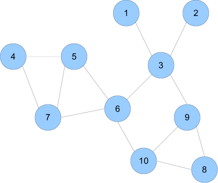
Figure 1: Network of ten people

In Cliqster, the generative model for the network is:

$$Y=\text{Bernoulli}(Z)$$ (1)

which means $Y(r,s)=Y(s,r)=1$ with probability $Z(r,s)$, and $Y(r,s)=Y(s,r)=0$ with probability $1-Z(r,s)$ for all $r>s$. Since the graph is undirected the matrix $Z$ is lower triangular.

Inspired by PCA and SVD, in Cliqster we choose to represent $Z$ in a new space chung96 , kim12 . Community structure is a key factor to understand and analyze a network, and because of this we are motivated to choose bases in a way that reflects the community structure hoff09 . Consequently, we decided to factorize $Z$ as

$$Z=\sum_{k=1}^{K}\mu_{k}B_{k}$$ (2)

where $K$ is the number of maximal cliques (bases), and $B_{k}$ is $k^{th}$ lower triangular basis matrix that represents the $k^{th}$ maximal clique, and $\mu_{k}$ is its contribution to the network. In section 3.4 we elaborate on this basis selection process. From this point forward, we consider these bases as cliques of a network. We also represent a network in this new space. Each network is parameterized by the coefficients and the bases which construct the $Z$, the network’s generating matrix.

3.2 Inference

When given a network $Y$ of people and their connections, our goal is to infer the parameters generating this network. We must first assume the bases are selected as baseline cliques. The likelihood of the network parameters (coefficients) given the observation is:

$$\mathcal{L}(\mu_{1:K})=\prod_{r>s:Y(r,s)=1}Z(r,s)\prod_{r>s:Y(r,s)=0}(1-Z(r,s))$$

We estimate these parameters by maximizing their likelihood under the constraint $0\leq Z(r,s)\leq 1$ for all $r>s$.

One can easily see the likelihood is maximized when $Z(r,s)=1$ if $Y(r,s)=1$ and $Z(r,s)=0$ if $Y(r,s)=0$. Therefore

$$Y=\sum_{k=1}^{K}\mu_{k}B_{k}$$ (3)

should be used for the lower triangle of $Y$.

Unfolding the above equation results in,

$$\begin{split}&Y(2,1)=\mu_{1}B_{1}(2,1)+\ldots+\mu_{K}B_{K}(2,1)\\ &Y(3,1)=\mu_{1}B_{1}(3,1)+\ldots+\mu_{K}B_{K}(3,1)\\ &Y(3,2)=\mu_{1}B_{1}(3,2)+\ldots+\mu_{K}B_{K}(3,2)\\ &\vdots\\ &Y(n,n-1)=\mu_{1}B_{1}(n,n-1)+\ldots+\mu_{K}B_{K}(n,n-1)\end{split}$$

We define two vectors,

$$\begin{split}&\boldsymbol{\mu}=(\mu_{1},\ldots,\mu_{K})^{\top}\\ &\boldsymbol{b^{rs}}=(B_{1}(r,s),\ldots,B_{K}(r,s))^{\top}\end{split}$$ (4)

So the new objective function can be written as,

$$J=\sum_{r>s}(\boldsymbol{\mu}^{\top}\boldsymbol{b^{rs}}-Y(r,s))^{2}$$ (5)

$J$ is convex with respect to $\mathbf{\mu}$ under the following constraints $0\leq\boldsymbol{\mu}^{\top}\boldsymbol{b^{rs}}\leq 1$. This is essentially a constrained least squares problem, which can be solved through existing efficient algorithms lawson1974solving , boyd2004convex . Through this formula, the representation parameters $\mu_{1:K}$ are thus computed easily and we are done with the inference procedure.

We turn our attention to the new representation and try to find an algorithm which can produce a more interpretable result. The exact generating parameters are no longer needed in our application. Therefore, by relaxing the constraints we will be able to present it with a simple and very efficient algorithm. In addition, the solution to this unconstrained problem provides us with an intuitive understanding of what is happening behind this inference procedure. To determine the optimal parameters, we must take the derivative with respect to $\mu$:

$$\frac{\partial J}{\partial\mathbf{\mu}}=2\sum_{r>s}\boldsymbol{b^{rs}}({\boldsymbol{b^{rs}}}^{\top}\boldsymbol{\mu}-Y(r,s))$$ (6)

By equating the above derivative to zero and doing a simple mathematical procedure, we are presented with the solution

$$\boldsymbol{\mu}=A^{-1}\boldsymbol{d}$$ (7)

where

$$\begin{split}&A=\sum_{r>s}\boldsymbol{b^{rs}}\boldsymbol{b^{rs}}^{\top}\\ &\boldsymbol{d}=\sum_{r>s}Y(r,s)\boldsymbol{b^{rs}}\end{split}$$ (8)

$A$ is a $K\times K$ matrix and $\boldsymbol{d}$ is a $K\times 1$ vector. Thus, while we still have a very small least squares problem, it has been significantly reduced from the original equation in which there were $O(n^{2})$ constraints. Despite this fact, we obtain very good results, and we will soon explain why this happens.

Our novel decomposition method finds $\mu$ which is used to represent a network, and which could stand-in for a network in network analysis applications. This representation is used in the next section in order to discriminate between different types of networks.

The results from the decomposition of the network presented in figure 1 is demonstrated in table 1.

Table 1: $\mu$ within each cluster

Cluster members	$\mu$
$\{8,9,10\}$	1.00
$\{5,6,7\}$	0.75
$\{4,5,7\}$	0.75
$\{1,2,3\}$	1.00
$\{6,10\}$	1.00
$\{3,9\}$	1.00
$\{3,6\}$	1.00

3.3 Interpretation

In general, it is not an easy task to interpret the Eigenvectors of an SVD. In our model, however, all the values of $A$ and $\boldsymbol{d}$ give you an intuition about the network. For further insight into this process, consider a matrix $A$. Every entry of this matrix is equal to the number of edges shared by the two corresponding cliques. This matrix encodes the power relationships between baseline clusters, as a part of network reconstruction. The intersection between two bases shows how much one basis can overpower another basis as they are reconstructing a network. In contrast, $\boldsymbol{d}$ presents the commonalities between a given network and its baseline communities. Through this equation, a community’s contribution to a network is encoded.

With the interpretation of this data in mind, the equation $A\boldsymbol{\mu}=\boldsymbol{d}$ is now more meaningful for understanding the significance of our new representation of a network. Consider multiplying the first row of the matrix by the vector $\boldsymbol{\mu}$, which should be equal to $\boldsymbol{d}_{1}$. In order to solve this equation, we have chosen our coefficients in such a way that when the intersection of cluster 1 and other clusters are multiplied by their corresponding coefficients and added together, the result is a clearer understanding of the first cluster’s contribution to the network construction.

3.4 Basis Selection

Users in persons of interest network usually form associations in particular ways, thus, community structure is a good distinguishing factor for different networks. There are different structures that form a community. One of the interesting structures that forms a community is the maximal cliques of that community. We use them as the basis of our method. There are so many ways to compute the maximal cliques of a network. We use the Bron-Kerbosch algorithm bron73 for identifying our network’s communities. As mentioned in azari12 , this is one of the most efficient algorithms for identifying all of the maximal cliques in an undirected network. After applying the Bron-Kerbosch algorithm to figure 1, we identify the communities that are represented in table 2. The Bron-Kerbosch algorithm is described in the algorithm 1.

Algorithm 1 Bron-Kerbosch algorithm

1:$C=\emptyset$ $\triangleright$ We keep the maximal clique in C

2:$I=V(G)$ $\triangleright$ The set of vertices that can be added to C

3:$X=\emptyset$ $\triangleright$ The set of vertices that are connected to C but are excluded from it

4:procedure Enumerate($C,I,X$)

5:     if $I==\emptyset$ and $X==\emptyset$ then

6:         $C$ is maximal clique

7:     else

8:         for each vertex v in I do

9:              $Enumerate(C\cup\{v\},I\bigcap N(v),X\bigcap N(v))$

10:              $I\leftarrow I\ \{v\}$

11:              $X\leftarrow X\cup\{v\}$               

The Bron-Kerbosch algorithm has many different versions. We use the version introduced in eppstein2011listing .

One of the most successful aspects of this algorithm is that it provides a multi-resolution perspective of the network. This algorithm identifies communities through a variety of scales, which, we will see, allows us to locate the most natural and representative set of coefficients and bases.

3.5 Complexity

The aforementioned inference equation requires $A$ and $\boldsymbol{d}$ to be computed, which can be done in $O(m+n)$ time where $m$ is the number of edges and $n$ is the number of nodes in the network. The least-square solution requires $O(K^{3})$ operations. A graph’s degeneracy measures its sparsity and is the smallest value $f$ such that every nonempty induced subgraph of that graph contains a vertex of degree at most $f$ lick70 . In eppstein2011listing they proposed a variation of the Bron-Kerbosch algorithm, which runs in $O(fn3^{f/3})$ where $f$ is a network’s degeneracy number. This is close to the best possible running time since the largest possible number of maximal cliques in an n-vertex graph with degeneracy $f$ is $(n-f)3^{f/3}$ eppstein2011listing .

A power law graph is a graph in which the number of vertices with degree $d$ is proportional to $x^{\alpha}$ where $1\leq\alpha\leq 3$. When $1<\alpha\leq 2$ we have $f=O(n^{1/2\alpha})$, and when $2<\alpha<3$ we have $f=O(n^{(3-\alpha)/4})$ buchanan13 . Combining with the running time, $O(fn3^{f/3})$ of the Bron-Kerbosch variant eppstein2011listing , we find that the running time for finding all maximal cliques in a power law graph to be $2^{O(\sqrt{n})}$.

However, the maximum number of cliques in graphs based on real world networks is typically $O(\log n)$ azari12 .

4 Results

In this section we investigate the properties of the new features we have learned about the network in question. Firstly, we introduce the new dataset we have built. Our experiments attempt to prove two claims:

1. the new representation is concise, and

2. it can discriminate between different network types

We will now compare our results with SVD decomposition and graphlet decomposition algorithms azari12 .

4.1 Dataset

We have gathered a dataset by gathering and fusing information from a variety of public and commercial sources. Our final dataset was comprised of around 750,000 persons of interest with 3,000,000 connections among them. We then filtered this dataset to slightly less than 550,000 individuals who fell into one of the following 5 categories:

1. Suspicious Individuals: Persons who have appeared on sanctioned lists, been arrested or detained, but not been convicted of a crime.

2. Convicted Individuals: Persons who have been indicted, tried and convicted in a court of law.

3. Lawyers/Legal Professionals: Persons currently employed in a legal profession.

4. Politically Exposed Persons: Elected officials, heads of parties, or persons who have held or currently hold political positions now or in the past.

5. Suspected Terrorists: Persons suspected of aiding, abetting or committing terrorist activities.

This dataset is publicly available at data .

Table 2: Table of Categories and corresponding sizes plus number of connected components and density of each category

Category	Members	Components	Density
Suspicious Individuals	316,990	77,811	0.0000180
Convicted Individuals	165,411	35,517	0.0000427
Lawyers/Legal Professionals	3,723	1,492	0.0006220
Politically Exposed Persons	13,776	4,947	0.0001533
Suspected Terrorists	31,817	5,016	0.0002068

The color scheme we use for our figures are as follow: Red for Suspicious Individuals (SI), blue for Convicted Individuals (CI), brown for Lawyer/Legal Professionals (LL), orange for Politically Exposed Persons (PEPS), and black for Suspected Terrorists (ST) .

4.2 Basic properties

We want to know whether our dataset has the common properties of social networks or not, i.e. having a power law distribution. The first thing to check is the degree distribution of each subnetwork, and if they can be fitted to a power-law distribution. We have a scale-free network If the degree distributions in our subnetwork follow power-law distribution. We used the poweRlaw powerlaw and igraph igraph packages to calculate the maximum likelihood power law fit of the Legal subnetwork, and the results are shown in figure 2. It looks like a scale-free network, but we need to check this with more accurate measures. In a power-law distribution $P(X=x)$ is proportion to $cx^{\alpha}$. The $\alpha$ of each subnetwork can be seen in the table 3. Each of our subnetwork can be fitted into a power-law distribution, so all of them are scale-free networks. However, these networks are not small-world networks. The number of connected components in each network, indicates if you start at a certain node in each network it is impossible to reach to most of the other nodes in that network.

Table 3: Table of alpha, the exponent of the fitted power-law distribution in each category

Category	$\alpha$
Suspicious Individuals	1.838563
Convicted Individuals	1.733839
Lawyers/Legal Professionals	2.977307
Politically Exposed Persons	3.107326
Suspected Terrorists	1.770715

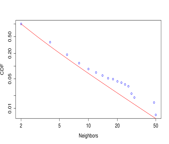
Figure 2: The cumulative distribution functions and their maximum likelihood power law fit of the Legal subnetwork

4.3 Sampling method

For each category we choose a random induced sub-graph of a $1,000$ vertices as a sample. We then analyze this data, and repeat this operation $1,000$ times and represent the data’s average with bold lines in the following graphs. All figures also include a representation of what happens to this data when the standard deviation of it is taken at a margin of 2 , which we illustrate through a line of a lighter variation of the same color. We analyzed this data with three different methods, the Singular Value Decomposition, Graphlet Decomposition, as well as our own proposed model.

4.4 Singular Value Decomposition

We first analyzed our data using the Singular Value Decomposition method chung96 . Figure 3 shows the effective number of non-zero coefficients for this algorithm. Figure 4 demonstrates the ability of this algorithm to discriminate between two different categories. Finally, the ability of the algorithm to distinguish between the 5 categories is illustrated in figure 5. The average number of bases we observed in the samples of a $1,000$ vertices is around $800$ as can be seen in figures 3, 4 and 5.

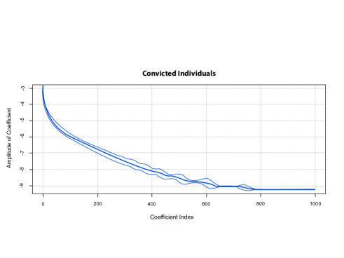
Figure 3: Number of bases and amplitude of coefficient for Convicted Individuals using SVDNumber of bases and amplitude of coefficient for Convicted Individuals using SVD

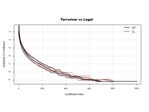
Figure 4: Comparison of coefficients between Terrorist sub networks and Legal sub networks using SVD

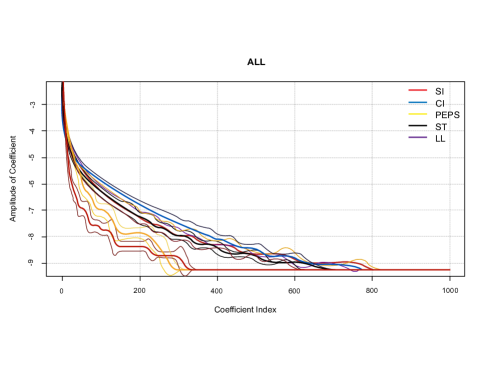
Figure 5: The ability of SVD method to distinguish between different categories of networks

4.5 Graphlet Decomposition

We next performed the same tests using Graphlet Decomposition. Figure 6 demonstrates the effective number of non-zero coefficients for this algorithm. Figure 7 shows the ability of this algorithm to discriminate between two different types of networks. The algorithm’s ability to distinguish between the 5 categories is again illustrated in figure 8. As can be seen in these figures the number of bases elements for Graphlet Decomposition is around $20$.

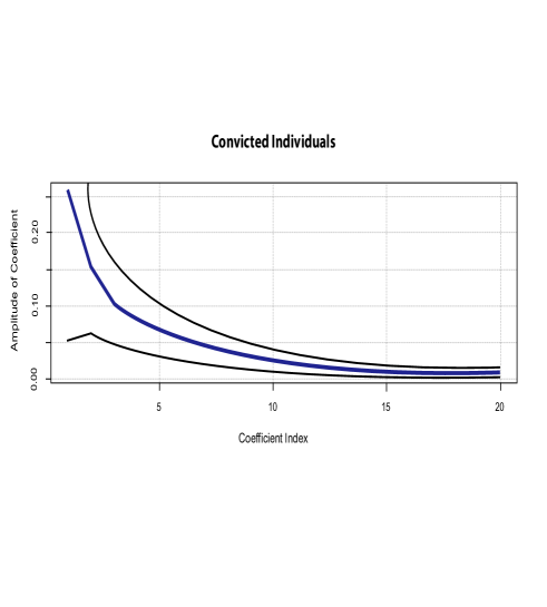
Figure 6: Number of bases and amplitude of coefficient for Convicted Individuals using Graphlet Decomposition Algorithm

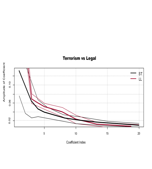
Figure 7: Comparison of coefficients between Terrorist sub networks and Legal sub networks using Graphlet Decomposition Algorithm

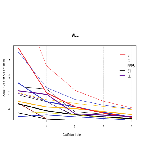
Figure 8: The ability of Graphlet method to distinguish between different categories of networks

4.6 Cliqster

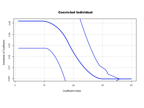
Figure 9: Number of bases and amplitude of coefficient for Convicted Individuals using Cliqster

Figure 10: Comparison of coefficients between Terrorist sub networks and Legal sub networks using Cliqster

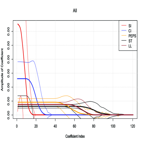
Figure 11: The ability of Cliqster to distinguish between different categories of networks

Finally, we performed the same tests using our method. We first determined appropriate bases using the Bron-Kerbosch algorithm. We then computed $A$ and $\boldsymbol{d}$. The new representation for a sample network of one category that resulted from our new method is shown in Figure 9. Figure 10 shows the ability of our algorithm to discriminate between two different types of networks. Our new algorithm’s ability to distinguish between two different types of networks is illustrated in Figure 11, which also shows that the number of bases elements for Graphlet Decomposition is around $50$.

4.7 Performance

We analyzed the time complexity of Cliqster in the section 3.5. Now it’s time to check if the empirical results verify our theory. For the Convicted Individuals subnetwork we ran both our method and SVD using the igraph package in R. The performance of the Graphlet method is very similar to Cliqster so we do not include that in this experiment.

We ran our experiment on “Intel(R) Core(TM) i7-2600 CPU @ 3.40GHz (8 CPUs),  3.4GHz” processor with “16384MB” of memory. As you can see in figure 12, as we grow the sample size our method performs twice as fast as the SVD method.

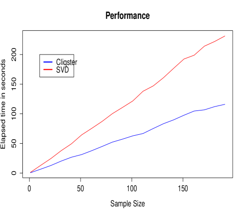
Figure 12: Comparison of performance between Cliqster and SVD

4.8 Distinguishability

In order to compare the ability of each of these methods to distinguish between different types of social networks, we sampled $100$ networks from each category, combining all of these samples before running the K-means clustering algorithm (with $5$ as the number of clusters), and repeated this action $100$ times. We used each network’s top $20$ largest coefficients, and are willing to know if coefficients of different sub-networks can be distinguished from each other. We gave the combined coefficients of all different sub-networks to the K-means clustering algorithm as an input, and calculated the mean error of clustering. As you can see in table 4, our method often returns the bases with the best ability to distinguish between the type of social network presented. The Graphlet Decompostion slightly outperforms our method in two of the following sub-networks, and such difference is negligible in practice.

Table 4: Mean error of clustering with $20$ coefficients ($\mu_{1:20}$)

Category	SVD	Graphlet	Cliqster
SI	0.51461	0.00817	0.0177
CI	0.71080	0.11535	0.0141
LL	0.75006	0.10931	0.0153
PEPS	0.66082	0.12195	0.0114
ST	0.65381	0.01303	0.0176

4.9 Classification

Another method for checking the ability of Cliqster to produce the features that can distinguish between different networks, is to use $k-$nearest neighbors algorithm (or $k-NN$ for short). $k-NN$ is a non-parametric method that is used for classification in a supervised setting. Let’s assume we want to compare the features that are used to distinguish between these two groups: Suspicious Individuals and Convicted Individuals. We train Cliqster with samples of size $1,000$ that are randomly selected from both communities, gather the features and repeat this operation $1,000$ times. After that we run the $k-NN$ with $k=3$ and a test data of size $100$. In order to avoid ties, we need to pick an odd number for $k$ in case of binary classification. When we set $k=3$ we are looking at the classification problem in a 3 dimensional space. We also make sure there is no intersection between the members of training and test sets to avoid the problem of over-fitting.

Figure 13 shows the result of this experiment. With using a training set of size $40$ we can classify these two groups with an accuracy of $97\%$. It basically means that when we have a training set of size 40, K-NN can learn how to distinguish between these two groups with an accuracy of $97\%$.

Things are a little bit different when it comes to comparing the behavior of Lawyers/Legal professionals network and Politically Exposed Persons network. As you can see in figure 14 we need a training set of size $100$ to reach to an accuracy of $74\%$. This difference suggest a contrast between the characteristics of these networks. According to Cliqster, the network structure of Lawyers/Legal professionals and the network structure of Politically Exposed Persons have more in common than the network structure of Suspicious Individuals and the network structure of Convicted Individuals.

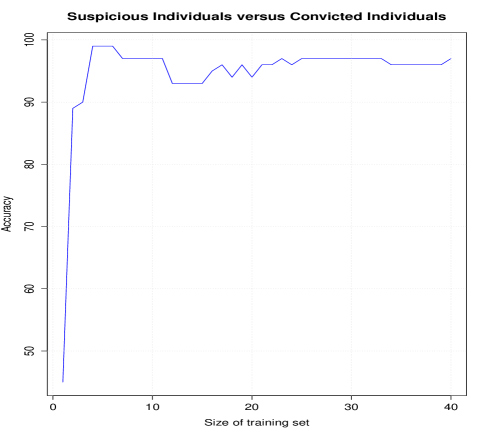
Figure 13: The accuracy of community detection based on the training size

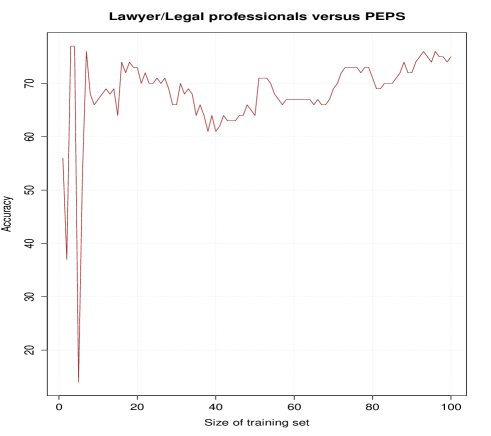
Figure 14: The accuracy of community detection based on the training size

If we analyze the network structure of Suspected Terrorists and compare it with network structure of Convicted Individuals, we will see that after using a training set of size around $20$ we reach to the $100\%$ accuracy. $k-NN$ can classify these two groups with no error 15. Now we compare the network structure of Suspected Terrorists and Politically Exposed Persons networks 16. After using a training set of size $50$, we reach to the $99\%$ accuracy.

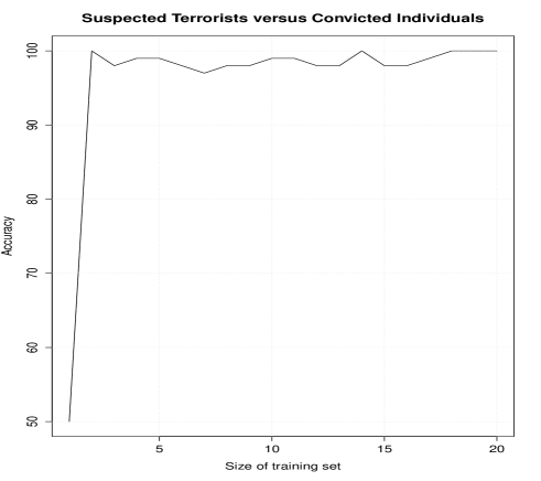
Figure 15: The accuracy of community detection based on the training size

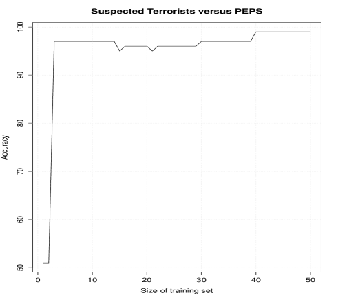
Figure 16: The accuracy of community detection based on the training size

4.10 Discussion

Figures 3, 6, and 9 compare the ability of the three methods to compress data. These graphs demonstrate that the SVD method is inefficient for summarizing a network’s features. The graph also shows that the Graphlet method produces the smallest feature space. Our representation is also very small, however, and the difference in size produced through these methods is negligible in real world applications of this equation. Earlier we demonstrated that the $20$ largest coefficients in the representation produced through our method is sufficient to outperform the Graphlet algorithm in terms of distinguish ability and clustering.

Figures 4, 7, and 10 demonstrate the ability of the algorithms to distinguish between two selected categories. When comparing our method with the SVD and Graphic Decomposition methods, the coefficients seem to be very similar between those produced by our method and the SVD method, however, our method also performs as well as the Graphlet Decomposition method in distinguishing between two types of networks. This demonstrates that community structure is a natural basis for interpreting social networks. By decomposing a network into cliques, our method provides an efficient transformation that is concise and easier to analyze than SVD bases, which are constrained through their requirement to be orthogonal. Figures 5, 8, and 11 verify these claims for all 5 categories.

Table 4 demonstrates the performance of our algorithm to consistently summarize each network according to category. We then clustered all coefficients using k-means. Through this process, it became clear that the SVD method could not identity the category of the network being analyzed. Because of this, we can infer that by selecting the community structure (cliques) as bases, our ability to identify a network is considerably improved. Our proposed algorithm was more accurate in clustering than the Graphlet Decomposition algorithm. Thus, the Bernoulli Distribution (as used in seminal work of Erdős and Rényi) is a simpler and more natural process for generating networks. Our proposed method is also easier to interpret and does not run the risk of getting stuck in local minima like the Graphlet method.

Finally, figures 13, 14, 16 and 15 demonstrate the ability of $k-NN$ to classify features produced by Cliqster in binary classification settings. They also give us some interpretations on similarities and differences between the network structure of different groups.

5 Conclusion

After proposing Cliqster, which is a new generative model for decomposing random networks, we applied this method to our new dataset of persons of interest. Our primary discovery in this research has been that a variant of our decomposition method provides a statistical test capable of accurately discriminating between different categories of social networks. Our resulting method is both accurate and efficient. We created a similar discriminant based on the traditional Singular Value Decomposition and Graphlet methods, and found that they are not capable of discriminating between social network categories. Our research also demonstrates community structure or cliques to be a natural choice for bases. This allows for a high degree of compression and at the same time preserves the identity of the network very well. The new representation produced through our method is concise and discriminative.

Comparing the three methods, we found that the dimensions of the Graphlet-bases and our bases were significantly smaller than the SVD-bases, while also accurately identifying the category of the network being analyzed. Therefore, our method is an extremely accurate and efficient means of identifying different network types.

On the non-technical side we would like to see how we can get law-enforcement agencies to adopt our methods. There are a number of directions for further research on the technical front. We would like to expand the use of our simple intuitive algorithm to weighted networks, such as networks with an edge generating process based on the Gamma distribution. The problem with the Maximum Likelihood solution for a network is that it is subject to over-fitting or a biased estimation. Adding a regularization term would adjust for this discrepancy. A natural choice for such a term would be a sparse regularization, which is in accordance with real social networks. Extensive possibility for future work exists in the potential of incorporating prior knowledge into Cliqster by using Bayesian inference. Another natural avenue for further investigations is to consider how Cliqster can be adapted to regular social networks.

References

- (1) S. Shokat Fadaee, M. Farajtabar, R. Sundaram, J. Aslam, and N. Passas, “The network you keep: Analyzing persons of interest using cliqster,” in Advances in Social Networks Analysis and Mining (ASONAM), 2014 IEEE/ACM International Conference on, Aug 2014, pp. 122–129.
- (2) UN. United nations. [Online]. Available: http://www.un.org/sc/committees/list_compend.shtml
- (3) T. Reuters. World-check. [Online]. Available: http://accelus.thomsonreuters.com/products/world-check-risk-intelligence
- (4) Interpol. [Online]. Available: http://www.interpol.int/
- (5) Dow jones factiva. [Online]. Available: http://www.dowjones.com/riskandcompliance/products.asp
- (6) OFAC. Office of foreign assets control. [Online]. Available: http://www.treasury.gov/resource-center/sanctions/SDN-List/Pages/default.aspx
- (7) Factcheck. [Online]. Available: http://www.dowjones.com/riskandcompliance/products.asp
- (8) RCMP. Royal canadian mounted police. [Online]. Available: http://www.rcmp-grc.gc.ca/index-eng.htm
- (9) Persons of interest dataset. [Online]. Available: http://www.ccs.neu.edu/home/saber/poi.RData
- (10) E. David and K. Jon, Networks, Crowds, and Markets: Reasoning About a Highly Connected World. New York, NY, USA: Cambridge University Press, 2010.
- (11) H. Azari Soufiani and E. M. Airoldi, “Graphlets decomposition of a weighted network,” Journal of Machine Learning Research, 2012.
- (12) A. Reiss, “Understanding changes in crime rates,” In Crime and Justice: A review of Research, vol. 10, 1980.
- (13) E. L. Glaeser, B. Sacerdote, and J. A. Scheinkman, “Crime and social interactions,” The Quarterly Journal of Economics, vol. 111, no. 2, pp. 507–48, May 1996.
- (14) E. Patacchini and Y. Zenou, “The strength of weak ties in crime,” European Economic Review, vol. 52, no. 2, pp. 209 – 236, 2008.
- (15) P. Erdős and A. Rényi, “On random graphs,” Publicationes Mathematicae Debrecen, vol. 6, pp. 290–297, 1959.
- (16) E. N. Gilbert, “Random graphs,” The Annals of Mathematical Statistics, vol. 30, no. 4, pp. 1141–1144, 1959.
- (17) E. M. Airoldi, “Bayesian mixed-membership models of complex and evolving networks,” DTIC Document, Tech. Rep., 2006.
- (18) G. Robins, P. Pattison, Y. Kalish, and D. Lusher, “An introduction to exponential random graph (p*) models for social networks,” Social Networks, vol. 29, no. 2, pp. 173 – 191, 2007, special Section: Advances in Exponential Random Graph (p*) Models.
- (19) M. Bilgic, L. Licamele, L. Getoor, and B. Shneiderman, “D-dupe: An interactive tool for entity resolution in social networks,” in Visual Analytics Science and Technology (VAST), Baltimore, October 2006.
- (20) G. Barta, “A link-based approach to entity resolution in social networks,” CoRR, vol. abs/1404.3017, 2014.
- (21) Y.-C. Lo, J.-Y. Li, M.-Y. Yeh, S.-D. Lin, and J. Pei, “What distinguish one from its peers in social networks?” Data Mining and Knowledge Discovery, vol. 27, no. 3, pp. 396–420, 2013.
- (22) Y. Yang, J. Tang, C. W.-k. Leung, Y. Sun, Q. Chen, J. Li, and Q. Yang, “Rain: Social role-aware information diffusion,” 2014.
- (23) W. E. Moustafa, A. Kimmig, A. Deshpande, and L. Getoor, “Subgraph pattern matching over uncertain graphs with identity linkage uncertainty,” CoRR, vol. abs/1305.7006, 2013.
- (24) K. Henderson, B. Gallagher, T. Eliassi-Rad, H. Tong, S. Basu, L. Akoglu, D. Koutra, C. Faloutsos, and L. Li, “Rolx: Structural role extraction & mining in large graphs,” in Proceedings of the 18th ACM SIGKDD International Conference on Knowledge Discovery and Data Mining, ser. KDD ’12. New York, NY, USA: ACM, 2012, pp. 1231–1239.
- (25) Y. Zhao, G. Wang, P. S. Yu, S. Liu, and S. Zhang, “Inferring social roles and statuses in social networks,” in Proceedings of the 19th ACM SIGKDD International Conference on Knowledge Discovery and Data Mining, ser. KDD ’13. New York, NY, USA: ACM, 2013, pp. 695–703.
- (26) R. A. Rossi and N. K. Ahmed, “Role discovery in networks,” IEEE Transactions on Knowledge and Data Engineering, vol. 99, no. PrePrints, p. 1, 2014.
- (27) K. Li, S. Guo, N. Du, J. Gao, and A. Zhang, “Learning, analyzing and predicting object roles on dynamic networks,” in Data Mining (ICDM), 2013 IEEE 13th International Conference on, Dec 2013, pp. 428–437.
- (28) S. Bhagat, G. Cormode, and S. Muthukrishnan, “Node classification in social networks,” CoRR, vol. abs/1101.3291, 2011.
- (29) H. Xu, Y. Yang, L. Wang, and W. Liu, “Node classification in social network via a factor graph model,” in Advances in Knowledge Discovery and Data Mining, ser. Lecture Notes in Computer Science, J. Pei, V. Tseng, L. Cao, H. Motoda, and G. Xu, Eds. Springer Berlin Heidelberg, 2013, vol. 7818, pp. 213–224.
- (30) K. Nowicki and T. A. B. Snijders, “Estimation and prediction for stochastic blockstructures,” Journal of the American Statistical Association, vol. 96, no. 455, pp. 1077–1087, 2001.
- (31) E. M. Airoldi, D. M. Blei, S. E. Fienberg, and E. P. Xing, “Mixed membership stochastic blockmodels,” Journal of Machine Learning Research, 2008.
- (32) B. Karrer and M. E. Newman, “Stochastic blockmodels and community structure in networks,” Physical Review E, vol. 83, no. 1, p. 016107, 2011.
- (33) A. Goldenberg, A. X. Zheng, S. E. Fienberg, and E. M. Airoldi, “A survey of statistical network models,” ArXiv e-prints, dec 2009.
- (34) F. R. K. Chung, “Spectral graph theory,” American Mathematical Society, 1997.
- (35) P. Hoff, “Multiplicative latent factor models for description and prediction of social networks,” Computational & Mathematical Organization Theory, vol. 15, no. 4, pp. 261–272, 2009.
- (36) M. Kim and J. Leskovec, “Multiplicative attribute graph model of real-world networks.” Internet Mathematics, vol. 8, no. 1-2, pp. 113–160, 2012.
- (37) C. L. Lawson and R. J. Hanson, Solving least squares problems. SIAM, 1974, vol. 161.
- (38) S. P. Boyd and L. Vandenberghe, Convex optimization. Cambridge university press, 2004.
- (39) C. Bron and J. Kerbosch, “Finding all cliques of an undirected graph,” Communications of the ACM, 1973.
- (40) D. Eppstein and D. Strash, “Listing all maximal cliques in large sparse real-world graphs,” in Experimental Algorithms. Springer, 2011, pp. 364–375.
- (41) D. R. Lick and A. T. White, “-degenerate graphs,” Canad. J. Math., vol. 22, pp. 1082–1096, 1970.
- (42) A. Buchanan, J. Walteros, S. Butenko, and P. Pardalos, “Solving maximum clique in sparse graphs: an algorithm for d-degenerate graphs,” Optimization Letters, 2013.
- (43) C. S. Gillespie, “Fitting heavy tailed distributions: The poweRlaw package,” Journal of Statistical Software, vol. 64, no. 2, pp. 1–16, 2015.
- (44) G. Csardi and T. Nepusz, “The igraph software package for complex network research,” InterJournal, vol. Complex Systems, p. 1695, 2006. [Online]. Available: http://igraph.org