Probing star formation in the dense environments of z$\sim$1 lensing halos aligned with dusty star-forming galaxies detected with the South Pole Telescope

Abstract

We probe star formation in the environments of massive ($\sim 10^{13}{\rm M}_{\mathord{\odot}}$) dark matter halos at redshifts of $z$$\sim$$1$. This star formation is linked to a sub-millimetre clustering signal which we detect in maps of the Planck High Frequency Instrument that are stacked at the positions of a sample of high-redshift ($z$$>$$2$) strongly-lensed dusty star-forming galaxies (DSFGs) selected from the South Pole Telescope (SPT) 2500 deg² survey. The clustering signal has sub-millimetre colours which are consistent with the mean redshift of the foreground lensing halos ($z$$\sim$$1$). We report a mean excess of star formation rate (SFR) compared to the field, of $(2700\pm 700)\thinspace{\rm M}_{\mathord{\odot}}\thinspace{\rm yr}^{-1}$ from all galaxies contributing to this clustering signal within a radius of $3\hbox{\hbox to0.0pt{.\hss}\kern 0.80002pt}^{\scriptstyle\prime}\hbox{\kern-0.29999pt}5$ from the SPT DSFGs. The magnitude of the Planck excess is in broad agreement with predictions of a current model of the cosmic infrared background. The model predicts that 80$\%$ of the excess emission measured by Planck originates from galaxies lying in the neighbouring halos of the lensing halo. Using Herschel maps of the same fields, we find a clear excess, relative to the field, of individual sources which contribute to the Planck excess. The mean excess SFR compared to the field is measured to be ($370\pm 40$)$\thinspace{\rm M}_{\mathord{\odot}}\thinspace{\rm yr}^{-1}$ per resolved, clustered source. Our findings suggest that the environments around these massive $z$$\sim$$1$ lensing halos host intense star formation out to about $2$ Mpc. The flux enhancement due to clustering should also be considered when measuring flux densities of galaxies in Planck data.

1 Introduction

Although it is known that the local environment of a galaxy impacts its star formation, the magnitude of the effect is unclear, particularly at high redshifts. Studies in the low redshift ($z\sim 0.1$) Universe show that star formation in galaxies is suppressed in highly dense environments such as in the centres of clusters, consistent with the effects of physical mechanisms such as ram-pressure stripping (e.g., Hogg et al., 2004; Blanton et al., 2005). However, the high-redshift picture is murkier. Some studies – for example, Elbaz et al. (2007), Cooper et al. (2008) and Popesso et al. (2011) – have found that the star formation rate (SFR)-density relation is either reversed or weaker at $z\sim 1$ than at $z\sim 0$. The picture that has emerged from these studies is one of galaxies that are still actively forming stars at $z\sim 1$ in high density environments such as the centres of groups. These may precede the formation of red, passive ellipticals that are observed in the centres of clusters at $z\sim 0$. However, not all studies agree. Feruglio et al. (2010) found no reversal of the SFR-density relation in the Cosmic Evolution Survey (COSMOS), and Ziparo et al. (2014) who investigated the evolution of the SFR-density relation up to $z\sim 1.6$ in the Extended Chandra Deep Field-South Survey (ECDFS) and the Great Observatories Origins Deep Survey (GOODS), also found no reversal.

In this paper, we target dense environments associated with massive ($M\gse 10^{13}{\rm M}_{\mathord{\odot}}$) dark matter lensing halos at $z$$\sim$$1$ and probe star formation in these dense environments. Our study falls into the context of a known correlation between the Cosmic Infrared Background (CIB, the thermal radiation from UV-heated dust in distant galaxies) and gravitational lensing (see, e.g., Blake et al., 2006; Wang et al., 2011; Hildebrandt et al., 2013; Holder et al., 2013; Planck Collaboration XVIII, 2014). To select the dense environments, we start with a sample of high-redshift ($z>2$) strongly-lensed dusty star-forming galaxies (DSFGs) discovered with the South Pole Telescope (SPT, Carlstrom et al., 2011). These DSFGs have been strongly lensed by foreground, massive early-type galaxies at $z$$\sim$$1$ which trace high-density environments (Hezaveh et al., 2013; Vieira et al., 2013). Our approach is to stack the Planck maps at the positions of the SPT DSFGs and search for an excess of far-infrared emission, relative to the field, in the environments of these foreground halos.

The stacked image contains the sum of a number of astrophysical components: (1) the parent sample of SPT DSFGs, (2) the mean background from the CIB (Lagache et al., 2005; Dole et al., 2006), (3) high-redshift sources clustered around the DSFGs, and (4) foreground sources associated with and clustered around the lensing halo. The first component should be unresolved relative to the point spread function (PSF) of the Planck map, and the second component should be a flat DC component in the map. The latter two clustered components would manifest themselves as a radially dependent excess relative to the Planck PSF. We use higher-resolution Herschel maps to isolate the emission from the background DSFGs and from the clustered signal. Planck is well suited to characterising this clustering signal because the beam size of Planck is well matched to the angular scale of the excess signal (e.g., Fernandez-Conde et al., 2008, 2010; Berta et al., 2011; Béthermin et al., 2012c; Viero et al., 2013b), and its wide frequency coverage enables an estimate of its mean redshift. At $z$$\sim$$1$, the Planck beam probes physical scales of around 2 Mpc. In the context of the halo model (Mo & White, 1996; Sheth & Tormen, 1999; Benson et al., 2000; Sheth et al., 2001), on these scales, we are probing both the ‘one-halo term’ (which is due to distinct baryonic mass elements that lie within the same dark matter halo and which describes the clustering of galaxies on scales smaller than the virial radius of the halo), and the ‘two-halo term’ (due to pairs of galaxies in separate halos and which gives rise to galaxy clustering on larger scales).

The paper is structured as follows. In Sect. 2, we describe the SPT DSFG sample and the ancillary data that we use for the analysis. We describe our methods in Sect. 3. We show the results in Sect. 4, which is split into two parts. The first part (Sect. 4.1) presents the excess of flux density we observe in the Planck stacks we construct relative to the flux densities from higher-resolution data at the same frequencies. We measure the clustered component from the Planck stacks, quantify the clustering contamination, obtain an SED and mean photometric redshift of the clustered component, derive a corresponding far-infrared (FIR) luminosity and SFR, and show the radial profiles of the various components of the Planck stack. In the second part (Sect. 4.2), we use Herschel/SPIRE observations to search for the individual sources that are responsible for the Planck excess and to constrain the nature of these sources. In Sect. 5, we interpret the Planck excess using a model of the CIB that relates infrared galaxies to dark matter halos. We discuss the implications of our results in Sect. 6 and present our conclusions in Sect. 7. Some supporting analyses and descriptions are presented in the Appendix. We refer to frequency rather than wavelength units throughout this paper. We use a $\Lambda$CDM cosmology with $H_{0}=70\thinspace\mathrm{km}\thinspace\mathrm{s}^{-1}\mathrm{Mpc^{-1}}$, $\Omega_{\mathrm{M}}=0.27$ and $\Omega_{\Lambda}=0.73$.

Table 1: SPT survey parameters and the DSFG sample used in this analysis

Sky coverage in SPT main survey	$2500\thinspace{\rm deg}^{2}$
Spatial resolution at 220 GHz	1$\arcmin$
Sensitivity at 220 GHz	$3.4-4.5\thinspace{\rm mJy}\thinspace{\rm beam}^{-1}$ rms
Main sample: number of DSFGs with $S_{220}>20$ mJy	65
Number of DSFGs observed with APEX/LABOCA	65
Number of DSFGs detected in APEX/LABOCA and with measured LABOCA flux densities	61
Number of DSFGs observed with Herschel SPIRE	65
Number of DSFGs detected in Herschel SPIRE and with measured SPIRE flux densities	62
Number of DSFGs detected in Herschel SPIRE and with ALMA 100 GHz positions	26

2 Data

2.1 South Pole Telescope selection

The South Pole Telescope (SPT, Carlstrom et al., 2011) is a 10-metre diameter millimetre/submillimetre (mm/sub-mm) telescope located at the geographic South Pole and is designed for low-noise observations of diffuse, low-contrast sources such as primary and secondary anisotropies in the cosmic microwave background (CMB, e.g., Reichardt et al., 2012; Story et al., 2013). The first generation SPT-SZ camera was a 960-element, three-band (95, 150 and 220 GHz) bolometric receiver. The sensitivity and angular resolution of the SPT make it an excellent instrument for detecting extragalactic sources of emission (Vieira et al., 2010).

The observations, data reduction, flux calibration, and generation of the extragalactic millimetre-wave point source catalogue are described in Vieira et al. (2010) and Mocanu et al. (2013). Sources detected in the SPT maps were classified as dust-dominated or synchrotron-dominated based on the ratio of their 150 GHz and 220 GHz flux densities. Approximating the spectral behaviour of sources between 150 GHz and 220 GHz as a power law, $S_{\nu}\propto\nu^{\alpha}$, we estimated the spectral index $\alpha$ for every source. A spectral index $\alpha\simeq 3$ is typical for sources dominated by dust emission while $\alpha\simeq-$1 is typical for the synchrotron-dominated population (see Vieira et al., 2010, for details). The sample of DSFGs used here is selected from the full 2500 deg² SPT source catalog using a cut on the raw 220 GHz flux density ($S_{220}>20$ mJy) and on spectral index ($\alpha>1.66$). In addition, sources also found in the Infrared Astronomy Satellite Faint-Source Catalogue (IRAS-FSC, Moshir et al., 1992), which are typically at $z\ll 1$ (median $\langle z\rangle=0.003$), were removed from the sample, leaving a population of bright, dust-dominated galaxies without counterparts in IRAS.

In this work, our parent sample comprises 65 DSFGs discovered by SPT over 2500 ${\rm deg}^{2}$ (Vieira et al., 2010). The 220 GHz source selection in this work exploits the nearly redshift-independent selection function of DSFGs at this frequency (e.g., Blain et al., 2002). The mean redshift of the SPT sample is $\langle z\rangle=3.5$, as determined by Weiß et al. (2013) through a CO redshift survey conducted with ALMA for a sample of 26 of these DSFGs. ALMA has now confirmed that the majority of the SPT DSFGs are strongly lensed (Hezaveh et al., 2013; Vieira et al., 2013). The lensing dark matter halos which are aligned with the SPT DSFGs are empirically observed to lie in the redshift range $z\sim 0.1$–$2.0$, in agreement with the theoretical prediction of $\langle z_{\rm lens}\rangle=1.15$ (with a $FWHM=1.53$) from Hezaveh & Holder (2011). Table 1 summarizes the SPT sample selection, the SPT sky coverage and depths, and the number of sources with ancillary observations that were used in this analysis. These include Herschel/SPIRE, APEX/LABOCA and ALMA imaging, the latter used to obtain accurate positions of the SPT sources in the analysis. The ancillary observations are described more fully below.

2.2 Planck

Planck (Tauber et al., 2010; Planck Collaboration I, 2011, 2014) is the third space mission to measure the anisotropy of the CMB. It observed the sky in nine frequency bands covering $28.5-857$ GHz with high sensitivity and angular resolution from 32.^′24 to 4.^′33. The High Frequency Instrument (HFI Lamarre et al., 2010; Planck HFI Core Team, 2011; Planck Collaboration VI, 2014) covered the 100, 143, 217, 353, 545, and 857 GHz bands with bolometers cooled to 0.1 K. In the present work we use the public Planck HFI maps, which can be obtained from the Planck Legacy Archive. The HFI data come from the nominal mission acquired between 13 August 2009 and 27 November 2010. These are converted from units of thermodynamic temperature to intensity units (${\rm MJy}\thinspace{\rm sr}^{-1}$, Planck Collaboration IX, 2014). From the full-sky Planck HEALpix maps (Górski et al., 2005) with a resolution parameter $N_{\rm side}=2048$, we extract Planck patches (in the tangential plane, using a gnomic projection) corresponding to each SPT field. The pixel scale in these Planck patches is $1\arcmin$. We then extract $1^{\circ}\times 1^{\circ}$ cutouts around each SPT source, centred on the SPT-derived position of the source.

2.3 IRIS

We combine the Planck-HFI data with 3000 GHz IRIS photometry (Miville-Deschênes & Lagache, 2005). IRIS is a reduction of the IRAS 3000 GHz data (Neugebauer et al., 1984) that benefits from an improved zodiacal light subtraction, and from a calibration and zero level which are compatible with the Diffuse Infrared Background Experiment (DIRBE), and from better de-striping. At 3000 GHz, IRIS maps are a significant improvement compared to the Schlegel et al. (1998) maps. The angular resolution of the maps is 4.3$\arcmin$. From the IRIS maps, we extract $1^{\circ}\times\thinspace 1^{\circ}$ cutouts of the SPT sources as in Sect. 2.2.

2.4 APEX continuum imaging

All the SPT sources from the $2500\thinspace{\rm deg}^{2}$ survey data were imaged at 345 GHz with the Large APEX BOlometer CAmera (LABOCA) at APEX. LABOCA (Siringo et al., 2009) is a 295-element bolometer array with a field-of-view of $11\hbox{\hbox to0.0pt{.\hss}\kern 0.80002pt}^{\scriptstyle\prime}\hbox{\kern-0.29999pt}4$ in diameter and an angular resolution of $19\hbox{\hbox to0.0pt{.\hss}}^{\scriptstyle\prime\kern-0.29999pt\prime}\hbox{\kern-0.70007pt}7$ (FWHM). The central frequency of LABOCA is $345\thinspace{\rm GHz}$ ($870\thinspace\mu{\rm m}$), with a passband FWHM of approximately 60 $\rm GHz$. The map size is approximately 12$\arcmin$. Observations were carried out under good weather conditions (median precipitable water vapour value of 0.9 mm, with a range of 0.3 mm to 1.5 mm) . The data reduction was performed in the same manner as in Greve et al. (2012). Sixty one of the 65 SPT sources in this study were detected in the LABOCA maps and had measured flux densities.

2.5 Herschel

We use Herschel Spectral and Photometric Imaging Receiver (SPIRE) observations of the SPT DSFGs in order to: (a) look for a statistical excess (relative to the field) of bright, individually detected sources that contribute to the Planck excess signal; (b) confirm that these bright, detected sources are associated with the $z\sim 1$ SPT lensing halos; and (c) estimate the mean contribution of these clustered sources to the excess of star formation that is observed in the environments around the lensing halos. The SPIRE instrument, its in-orbit performance and its scientific capabilities are described in Griffin et al. (2010), while its calibration methods and accuracy are outlined in Swinyard et al. (2010). We use two sets of SPIRE maps for this work.

• SPIRE $10\arcmin\times 10\arcmin$ maps: The SPIRE maps at 1200 GHz ($250\thinspace\mu$m), 857 GHz (350$\thinspace\mu$m), and 545 GHz (500$\thinspace\mu$m) used in this work were made from data taken during observing programmes OT1_jvieira_4, OT2_jvieira_5, DDT_mstrande_1 and DDT_tgreve_2 for the lensed SPT DSFGs that were selected from the 2500 deg² SPT survey. These maps had coverage complete to a radius of 5$\arcmin$ from the nominal SPT-derived position. More accurate positions of the SPT DSFGs were then obtained for the analysis on the SPIRE maps (see Sec. 2.6). The maps were produced via the standard reduction pipeline HIPE v9.0, the SPIRE Photometer Interactive Analysis package v1.7, and the calibration product v8.1. The median rms in these maps is 9.7 mJy at 1200 GHz, 8.9 mJy at 857 GHz and 9.9 mJy at 545 GHz. This is dominated by confusion noise (approximately 6 mJy in each band). All 65 SPT sources were imaged with SPIRE and 62 were detected and had measured flux densities.

• SPIRE observations of the Lockman–SWIRE field: We use archival SPIRE data from the Herschel Multi-tiered Extragalactic Survey (HerMES, Oliver et al., 2012) of the Lockman- SWIRE field centred on RA=10:48:00.00, Dec=$+$58:08:00.0 and 18.2 deg² in area . This data does not overlap with the SPT coverage but is used as a reference field in the analysis. The 5$\sigma$ confusion noise is 27.5 mJy at 857 GHz (Nguyen et al., 2010) and the total 5$\sigma$ noise (including instrumental noise) at 857 GHz is approximately 40 mJy.

2.6 ALMA

When performing the analysis on the Herschel/SPIRE images, we use the positions of the SPT DSFGs that were derived from ALMA 100 GHz (3 mm) continuum observations whenever they are available. Thus for 26 galaxies, we use the ALMA positions and for the remainder, we use the positions given by LABOCA. The ALMA positions used here were reported in Weiß et al. (2013).

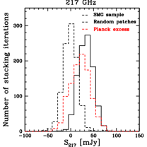
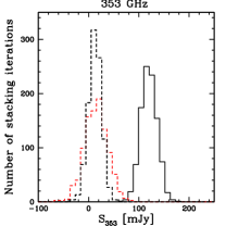
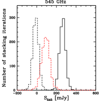
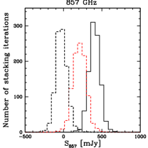
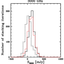
Figure 1: Distribution of Planck and IRIS flux densities from aperture photometry within a radius of $3\hbox{\hbox to0.0pt{.\hss}\kern 0.80002pt}^{\scriptstyle\prime}\hbox{\kern-0.29999pt}5$ over: (1) 1000 bootstrap realisations of stacking 65 $1^{\circ}\times 1^{\circ}$ patches of the SPT DSFGs (black solid line); (2) 1000 iterations of stacking the same number (65) of $1^{\circ}\times 1^{\circ}$ patches selected randomly from the Planck maps covering the SPT fields at 217, 353, 545, 857 GHz and from the IRIS maps at 3000 GHz (black dashed line); (3) 1000 bootstrap realisations of the Planck and IRIS excess after removing the high redshift compact source (the SPT DSFGs) from the stacked map in each realisation using the formalism in Appendix D (red dashed line). At 217 and 3000 GHz, there is a much larger number of stacks on random locations (black dashed line) which have flux densities that are as high as the flux densities of the stacks on the SPT sources (black solid line), compared to the other frequencies. The 353, 545, and 857 GHz channels are therefore cleaner.

3 Methods

In this section, we describe our methods for (1) stacking Planck HFI maps at the positions of the SPT DSFGs and performing photometry on the stacked maps and (2) performing source detection and photometry on the Herschel/SPIRE maps.

3.1 Stacking Planck maps at the locations of SPT DSFGs

The noise at the high frequencies in Planck is dominated by confusion noise from the CIB (Planck Collaboration XVIII, 2011). Stacking the Planck maps at the locations of SPT sources enables us to go beyond the confusion noise level that impacts individual detections of DSFGs (e.g., Dole et al., 2006). We also perform simulations to correct for a positional offset of the SPT DSFGs due to the effect of pixelization in the HEALPix scheme (see Appendix B).

We perform aperture photometry on the stacked maps at each Planck HFI frequency within a $3\hbox{\hbox to0.0pt{.\hss}\kern 0.80002pt}^{\scriptstyle\prime}\hbox{\kern-0.29999pt}5$ radius of the SPT DSFG locations. This corresponds exactly to the radius of the region over which we perform the Herschel detection and photometry of sources around the SPT DSFGs (see Sect. 3.2). We also investigated larger aperture sizes (up to a radius of 5$\arcmin$) and found that it produced no significant differences in the results.

We constrain the uncertainties on the average flux densities measured via stacking by performing 1000 bootstrap realizations of the stacked sample. Each bootstrap realization is constructed by randomly selecting, with replacement, 65 SPT sources, stacking their Planck maps, and measuring the flux density in the resulting image. The scatter is determined by the $68\%$ confidence level in the resulting flux density distribution. Fig. 1 shows the distribution of flux densities obtained after doing aperture photometry on bootstrap realizations of these stacked maps at each Planck frequency and at the IRIS frequency. Also shown, for the same frequencies, are the flux density distributions (again after doing aperture photometry with a 3.5$\arcmin$ aperture radius) for 1000 iterations of stacking the same number (65) of $1^{\circ}\times 1^{\circ}$ maps which are selected randomly in the Planck sky of the SPT fields. The flux density distributions that result from this null test are all peaked around zero, as expected, and at 353, 545, and 857 GHz, are quite distinct from the distribution of flux densities obtained from the 1000 bootstrap realizations of stacking maps at the positions of the 65 SPT DSFGs. However, at 217 and 3000 GHz, there is a much larger number of stacks in the null test which have flux densities that are as high as those derived from the bootstrap realizations on the SPT sources, compared to the other frequencies. This is due to fluctuations of the Galactic cirrus at 3000 GHz and of the CMB at 217 GHz in the stacked Planck and IRIS maps.

Our paper therefore focuses on the signal from 857, 545, and 353 GHz. In Appendix A, we show that the bootstrap and photometric uncertainties in the Planck flux densities are similar and that the uncertainty due to inhomogeneity in the SPT sample is negligible. We will use the bootstrap uncertainties throughout the analysis.

3.2 Herschel source detection and photometry

We create $10\arcmin$-by-$10\arcmin$ maps centred on the SPT DSFGs in each SPIRE band. Due to the short size of the scan pass ($10\arcmin$), the mapmaker does not accurately recover angular scales as large as several arcminutes. This means that these maps are poorly suited to recovering the clustering signal on $3\hbox{\hbox to0.0pt{.\hss}\kern 0.80002pt}^{\scriptstyle\prime}\hbox{\kern-0.29999pt}5$ scales (as was done with Planck). Therefore we focus on individually detected sources in the SPIRE maps.

We extract the resolved sources in the SPIRE maps as well as in the blank HerMES Lockman-SWIRE field (which was used as a reference field) in order to verify that there is indeed an excess of resolved sources that contribute to the large-scale clustering signal observed by Planck. We use the STARFINDER algorithm (Diolaiti et al., 2000) which was developed to blindly extract sources from confused maps, for this purpose. In order to avoid an extraction bias (which can vary with position in the maps), we consider only high significance detections: $S_{857}>50\thinspace$mJy, approximately $6\sigma$ in the HerMES Lockman SWIRE field and in the SPIRE maps of the SPT sources.

The coverage of the maps of the SPT sources is not homogeneous. We only extract sources within $3\hbox{\hbox to0.0pt{.\hss}\kern 0.80002pt}^{\scriptstyle\prime}\hbox{\kern-0.29999pt}5$ of the SPT DSFG in order to minimize the effect of inhomogeneity. We have also verified that small changes to this radius (between 2.5$\arcmin-$3.5$\arcmin$) do not impact our results. We do not use the $S_{545}/S_{857}$ colours in the analysis because the 600 GHz ($500\thinspace\mu$m) maps (beam FWHM$=$36$\arcsec$) suffer from a larger degree of source confusion than the 1200 GHz (FWHM$=$18$\arcsec$) and 857 GHz (FWHM$=$25$\arcsec$) maps. Hence we focus on the $S_{857}$/$S_{1200}$ colours in this work.

We compute $S_{857}/S_{1200}$ colours of these 857 GHz-flux-selected galaxies using two different methods, depending on whether or not they are detected independently at 1200 GHz. For objects detected at both frequencies, we take the flux densities reported by STARFINDER at each frequency. Some red objects are not detected at 1200 GHz. For these galaxies, we measure the 1200 GHz flux density at the 857 GHz position using FASTPHOT (Béthermin et al., 2010b), which is designed to deblend sources with known positions. To obtain the most accurate flux densities possible, we also add the other sources in the same field, which are detected at 1200 and 857 GHz, to the list of positions used by FASTPHOT. In general, we recover source flux densities at 3$-$6 $\sigma$ (which is just below the blind detection threshold), and the precision on the colours is between 16.5 and 33.0$\%$. The same algorithm is applied to the maps of the SPT sources and the control field so as to have the same potential residual biases, since our goal is not to obtain an absolute measurement of the colour distribution, but to detect potential differences between the environment of SPT sources and blank fields. In order to check the quality of our source extraction we perform Monte Carlo simulations (Appendix C), injecting sources into both the maps of the SPT sources and the larger HerMES field. We check the output against input flux densities at each frequency. We also examine the completeness as a function of flux density, where completeness is defined as the fraction of recovered sources. For the rather conservative flux density cut at $S_{857}>50\thinspace$mJy, the completeness is higher than 95$\%$ and flux boosting (due to Malmquist and Eddington bias and from source confusion) is below 5$\%$ in both the maps of the SPT sources and the control field.

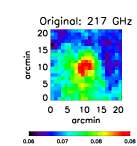
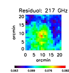
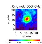
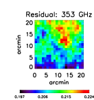
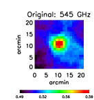
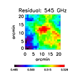
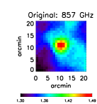
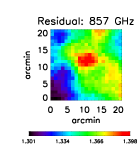
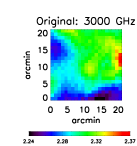
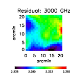
Figure 2: Left panel: Planck and IRIS maps, in units of MJy$sr^{-1}$ which are obtained by stacking individual maps at the positions of the SPT DSFGs. Each map in the stack is centred on the SPT-derived position of the DSFG. The original size of the stacked maps is $1^{\circ}\times 1^{\circ}$. Here, we zoom into the central $20\arcmin\times 20\arcmin$ region in order to show structure more clearly. The signal from the DSFGs is strong at 353, 545, and 857 GHz. Right panel: residual maps obtained after removing the central compact source from each stacked map using the formalism in Appendix D. These residual maps show an extended but isolated structure at 545 and 857 GHz.

4 Results

Here, we present our results in two broad divisions: (1) the measurement and analysis of the clustered component from stacking the Planck HFI maps at the locations of the SPT DSFGs; and (2) the confirmation, using Herschel observations, of the clustering signal and the nature of the sources contributing to this clustering signal.

4.1 The Planck excess

We present the results of the stacking analysis, including the measurement of the clustered component, its SED and photometric redshift, and we estimate the SFR of all the galaxies contributing to the signal. Finally, we present azimuthally-averaged profiles of the different components in the Planck stack.

4.1.1 Measuring the clustered component

The left panel of Figure 2 shows the Planck and IRIS maps which are stacked at the positions of the 65 SPT DSFGs. Figure 3 shows the mean spectral energy distribution (SED) of the sample that is derived from Planck and IRIS data after performing aperture photometry on the stacked maps (black squares and line). The dashed line in Fig. 3 is a model galaxy SED at $z=3.5$ generated from the SED library of Magdis et al. (2012). We observe that the mean SED of the sample that is derived from doing aperture photometry on the stacked maps is not simply a rescaling of a typical star-forming galaxy SED at $z=3.5$. As a comparison with the Planck flux density measurements, we also show the mean flux density measurements of the DSFGs (with the same selection in $S_{220}$) at higher resolution, at 220 GHz (the SPT measurement), 345 GHz (LABOCA), 545 GHz and 857 GHz (SPIRE). The LABOCA and SPIRE measurements shown in Fig. 3 are the mean flux densities for all SPT sources which were detected in the LABOCA and SPIRE maps respectively and which had measured flux densities (see Table 1). We observe an excess in the Planck flux density particularly at the highest frequencies, compared to the flux density from other observations at the same frequencies (albeit with relatively high uncertainties): $206\pm 73\thinspace$mJy at 857 GHz, $84\pm 31\thinspace$mJy at 545 GHz, and $36\pm 16\thinspace$mJy at 353 GHz. At 220 GHz, the excess is statistically not significant: $4\pm 16\thinspace$mJy.

One possible source of the excess in the Planck maps is sub-mm emission from sources clustered within the Planck beam. The stacked signal can therefore be decomposed into two components, a DSFG contribution and a clustered component. We consider two scenarios here:

• If the clustered component is at the same redshift as the DSFGs and consists itself primarily of DSFGs, the SEDs of both components should be very similar. In particular, the peaks of the SEDs will be at approximately the same frequencies. The excess will thus be constant in frequency modulo some noise due to dust temperature and emissivity variations.

• If the clustered component is at a lower redshift than the DSFGs, then the SED of the clustered component would be expected to peak at a higher frequency than the stacked DSFGs.

The trend of the measured excess signal with frequency is more consistent with the second scenario. This implies that the clustered signal within the Planck beam has a much larger contribution from low redshift sources than from any clustered sources in the neighborhood of the DSFGs. Given the fact that the majority of SPT DSFGs are lensed, their positions are correlated with massive dark matter halos at $z\sim 1$, so we expect to detect sub-mm emission from galaxies in the lensing halos.

We next test the hypothesis that there is a clustered signal within the $3\hbox{\hbox to0.0pt{.\hss}\kern 0.80002pt}^{\scriptstyle\prime}\hbox{\kern-0.29999pt}5$ radius aperture. We fit the stacked Planck maps to a model following the formalism of Béthermin et al. (2010b, 2012c) and Heinis et al. (2013). The model has 3 components: (1) the compact source, (2) the clustered component, and (3) the background.

The method is described fully in Appendix D. We use this formalism to extract the mean flux density of the compact source (red points and line in Fig. 3) by fitting simultaneously for all three components in the stack. The right panel of Figure 2 shows the residual maps after the compact source has been removed from the stacked maps using this formalism. The residual images at 545 and 857 GHz in particular show an extended but isolated structure around the centre of each map. The Planck excess is now defined as the difference between the compact source’s flux density and the total flux density within the $3\hbox{\hbox to0.0pt{.\hss}\kern 0.80002pt}^{\scriptstyle\prime}\hbox{\kern-0.29999pt}5$ radius aperture. The same excess is recovered if we perform aperture photometry on the residual maps at each frequency (see also Sect. 4.1.5, where we measure radial profiles of the different components).

In addition, at 217 GHz, since we have measured SPT flux densities for the full SPT DSFG sample, we remove a compact source from the Planck stack where the normalization of that compact source in the fit is fixed by the mean SPT flux density, and then perform aperture photometry on the residual map. This results in a statistical uncertainty in the mean Planck excess measured at 220 GHz that is lower than if we did not use this prior. At 353 GHz, as seen in Fig. 3, the total flux density in the stack and the flux density from the compact source that is obtained from the model fits, are $0.6\sigma$ apart, and we find no significant evidence for an excess. However, at higher frequencies, a clustered component is needed to reconcile the Planck flux densities with those obtained from the higher resolution observations in Fig. 3.

In Appendix E, we describe three tests to verify that the clustered component is real and not simply an artefact of the stacking procedure. In the first test (see Appendix E.1), we perform stacking simulations, with artificial compact source components and clustering components generated using the same model as in Appendix D and injected into blank Planck maps before they are stacked. We find no significant bias arising from the stacking procedure in the mean flux densities obtained from either aperture photometry or from fitting to the source and clustered components. In Appendix E.2, we also test whether the extended component seen in the residual maps at 545 and 857 GHz around the central compact source in Figure 2 is actually part of the structure in the background, by creating many realisations of the stacked maps where the individual Planck maps are rotated randomly by 90^∘ before they are stacked. The clustered component appears consistently at 545 and 857 GHz as an isolated structure around the compact source and is therefore not simply part of the structure in the background.

In Appendix E.3, we show that the clustering component does not appear at 545 and 857 GHz if there are no lensing halos in the foreground. We stack Planck and IRIS maps at the positions of a sample of 65 SPT synchrotron sources (Vieira et al., 2010). These sources are not angularly correlated with foreground structure and we find no extended component in the residual maps after removing the central compact source (the synchrotron source itself) from the stacked maps using the same fitting formalism. This suggests that the clustered component found in this study is specific to the foreground lensing halos of the STP DSFGs.

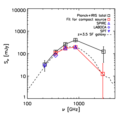
Figure 3: Comparison of the mean Planck (217$-$857 GHz) and IRIS (3000 GHz) flux densities of the SPT sample after stacking the Planck and IRIS maps (at the positions of the SPT DSFGs) with: (a) the mean SPT 220 GHz flux density of the sample (blue inverted triangle); (b) the mean APEX/LABOCA flux density at 345 GHz (blue diamond); and (c) the mean Herschel/SPIRE flux density at 857 GHz and 545 GHz (blue triangles). The mean Planck and IRIS flux densities are estimated from: (i) aperture photometry (black squares and line); and (ii) after fitting simultaneously for the source, clustering and background in the stacked Planck and IRIS maps using the formalism given in Appendix D (red squares and line). There is no fitted flux measurement of the compact source component shown at 217 GHz because we have SPT flux measurements for the full SPT sample and we use the mean SPT flux density at 220 GHz to constrain the fitting to the clustered term, as described in Sec. 4.1.1. Planck and IRIS photometric uncertainties are obtained by bootstraping ($N_{\rm boot}=1000$ over the stack). Also shown is an SED of a $z=3.5$ star-forming galaxy generated from the Magdis et al. (2012) effective templates (dashed line). The SED derived from aperture photometry in the stack (black line) is wider than this typical SED of a star-forming galaxy, because it is a superposition of the SEDs of a high redshift compact component and a low redshift clustered component. Subtracting the best-fit clustered term from the Planck flux densities brings them into agreement with the SPIRE and LABOCA flux densities.

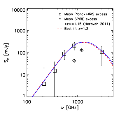
Figure 4: SED of the Planck excess (black squares), which is derived from the difference between the total flux density within a $3\hbox{\hbox to0.0pt{.\hss}\kern 0.80002pt}^{\scriptstyle\prime}\hbox{\kern-0.29999pt}5$ radius (black squares in Fig. 3) and the flux density of the compact source in the stack (red squares in Fig. 3). There is no significant evidence of an excess at 220 GHz or 353 GHz; the data are consistent with zero at 1$\sigma$. We also compare the Planck excess SED with two star-forming galaxy SEDs that are generated from the B12 library (Béthermin et al., 2012a) and redshifted to: (1) the predicted mean redshift ($z\sim 1.15$) of the SPT lensing halos in Hezaveh & Holder (2011) (blue line); (2) the best fitting redshift ($z\sim 1.2$) found by maximizing the probability distribution for the redshift $p(z)$ (red dashed line). The data requires $T_{d}>50$ K at 95$\%$ confidence if we assume the excess emission originates from $z=3.5$. On the other hand, if we assume $z=1.15$, we obtain $T_{\rm d}=(32\pm 19)$ K (in addition, $T_{\rm d}=(33\pm 20)$ K for $z=1.2$ from the best fit to the Planck excess) which is within the range of expected dust temperatures of galaxies (see Sect. 4.1.3). Finally, we show the mean excess of flux density $S_{\rm excess}$ at 857 GHz and 1200 GHz from sources that are detected in Herschel/SPIRE within $3\hbox{\hbox to0.0pt{.\hss}\kern 0.80002pt}^{\scriptstyle\prime}\hbox{\kern-0.29999pt}5$ of the SPT DSFGs. This excess in flux density is computed relative to all other sources that have been detected at the same flux density threshold in a larger control field (see Sect. 4.2 and Eq. 2). It is expected that the detected SPIRE sources account for a fraction (approximately 20% at 857 GHz) of the Planck excess (Béthermin et al., 2012c).

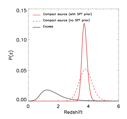
Figure 5: Probability distribution for the mean redshift, $p(z)$ for two components of the Planck stack. The dashed red line shows $p(z)$ for the compact source, where the SED is given by the red line in Fig. 3 which is obtained from the fit described in Appendix D using only the 353, 545, 857 and 3000 GHz data. The solid red line is the result of fitting to an SED where we also use a 217 GHz data point, assuming the compact source has the same mean flux density at 217 GHz as the SPT mean flux density of the sample. The black line shows $p(z)$ for the Planck excess, the SED for which is shown in Fig. 4 (see also the fifth row of Table 2). The quantity $p(z)$ for each component is derived by fitting SED templates from the Magdis et al. (2012) library in a range of redshifts, to the measured SED of that component, using Eqs. 13$-$15 (see Sect. 4.1.3 and Appendix F for details). The distribution $p(z)$ for the compact source component peaks near the mean of the redshift distribution for SPT sources $z\sim 2$–$6$ found in Weiß et al. (2013), whereas the $p(z)$ for the Planck excess has a maximum at $z=1.2$.

4.1.2 Clustering contamination in the stacked flux densities of the DSFGs

We quantify the contribution of the clustered component associated with the foreground lensing halos relative to the measured stacked flux densities of the high redshift lensed galaxies. The enhancement introduced by the clustering signal (Béthermin et al., 2010b; Kurczynski & Gawiser, 2010; Béthermin et al., 2012c; Bourne et al., 2012; Viero et al., 2013a) needs to be taken into account in order to obtain a correct estimate of the mean flux density of the background lensed galaxies in the stack. In this study, in particular, the clustering contamination is significant, because the beam size of Planck is comparable to the angular scale of the clustering signal. Our aim is therefore to quantify the clustering contamination in the different frequency channels of Planck HFI.

The relative clustering contamination can be expressed as the ratio of the flux density of the clustered component to the flux density of the compact source component in the stack. In Table 2, we list the mean flux densities of the clustered component and compact source component in the stack, as well as the relative clustering contamination for the 217, 353, 545, and 857 GHz channels. The flux densities of the compact source component and the clustered component are obtained from the fits. When fitting the clustered component at 217 GHz, however, we exploit the fact that we have measured SPT flux densities for the full SPT DSFG sample and introduce the mean SPT flux density in the fitting in order to compute the strength of the clustered term, as described in Sec. 4.1. At 217 GHz, therefore, the strength of the clustered term is defined as the flux density of the residual component obtained after removing a compact source (through the same fitting procedure) whose normalization is given by the mean SPT flux density itself.

We find that the relative clustering contamination has a large uncertainty at 220 GHz but thereafter increases with frequency in the Planck HFI channels (the beam FWHM is relatively stable among the HFI frequencies, so we focus on the frequency dependence here). This flux density contribution from sources clustered around the foreground lensing halos adds to the stacked flux density of the background lensed galaxies. This boosts the flux density estimates of the background galaxies that are derived from aperture photometry performed on Planck data. The clustering contamination should therefore be taken into account in order to obtain the correct flux densities of galaxies (both ensemble-averaged flux densities from stacking but also flux densities of individual galaxies) in Planck data.

Table 2: Mean flux densities of the components in the Planck stack and the relative clustering contamination values as a function of frequency. The latter is expressed as the ratio of the flux density of the Planck excess to the flux density of the compact source component. The flux density of the compact source component is expressed in two different ways: (1) from the high-resolution measurements (SPT, LABOCA and SPIRE: third row) assuming that there is negligible clustering of sources in the SPT, LABOCA and SPIRE beams; (2) from the fits to the components in the Planck stack, as described in Appendix D (fourth row). The flux density of the clustered component (fifth row) is then computed from the difference between the total flux density within a $3\hbox{\hbox to0.0pt{.\hss}\kern 0.80002pt}^{\scriptstyle\prime}\hbox{\kern-0.29999pt}5$ aperture and the fit to the compact source component. In addition, at 217 GHz, since we have measured SPT flux densities for the full SPT DSFG sample, we use the mean SPT flux density in order to constrain the strength of the clustered component at 217 GHz: we remove a compact source from the Planck stack where the normalization of that compact source in the fit is fixed by the mean SPT flux density, and then perform aperture photometry on the residual map. As we employ this prior based on the SPT flux density, we do not quote a value for the flux density of the compact source component at 217 GHz obtained from the fits. Finally, the relative clustering contamination is expressed as the ratio of the flux density of the clustered component to that of the compact source component, which are both obtained from the fits. At 217 GHz, this is computed as the ratio of: (1) the clustered component computed with the prior on the SPT flux density and (2) the SPT flux density itself.

Frequency	217 GHz	353 GHz	545 GHz	857 GHz
Total flux density from aperture photometry [mJy]	32.7$\pm$16.4	120.1$\pm$16.1	261.6$\pm$30.9	402.4$\pm$72.5
Flux density of the compact source component (high resolution measurements) [mJy]	28.8$\pm$0.7	84.1$\pm$0.9	177.5$\pm$2.0	196.7$\pm$2.4
Flux density of the compact source component (from fit) [mJy]	-	104.9$\pm$16.9	171.4$\pm$25.5	192.8$\pm$28.9
Flux density of the clustered component (from fit) [mJy]	3.9$\pm$16.4	15.2$\pm$23.3	90.1$\pm$40.1	209.6$\pm$78.0
Relative clustering contamination	0.1$\pm$0.6	0.2$\pm$0.2	0.5$\pm$0.2	1.1$\pm$0.4

4.1.3 SED and photometric redshift of the clustered component

In Fig. 4, we show the SED of the excess signal. In order to derive redshifts from the sub-mm SEDs, we use the effective SED library of Béthermin et al. (2012a), which is based on the Magdis et al. (2012, hereafter M12) SED libraries and the Béthermin et al. (2012a, hereafter B12) model. These templates are the luminosity-weighted average SED of all the galaxies described by the B12 model at a given redshift. There are two families of templates included – “main-sequence” (MS) and “starburst” (SB) galaxies – and both evolve with redshift. We also assume a scatter in the mean radiation field $\langle U\rangle$ of 0.2 dex (about 0.05 dex in the dust temperature) at fixed redshift for a given family of templates.

We fit the template SEDs as a function of redshift to the SED of: (1) the compact source; and (2) the Planck excess (after subtracting the contribution from the compact source). We derive the probability distribution for the redshift, $p(z)$, for these two components (see Appendix F for a full description of how $p(z)$ was computed), as shown in Fig. 5. The $p(z)$ of the compact source component is narrower than the redshift distribution from $z\sim 2$–$6$ found by Weiß et al. (2013) for a subset of the sources analysed here, but has a consistent central value at $z\sim 4$. The $p(z)$ of the excess is quite different and peaks at $z\sim 1.2$, with a tail to higher redshifts. In Fig. 4, we show the template SED redshifted to: (a) the best-fit redshift $z=1.2$; and (b) the theoretical mean redshift of the lensing halos ($z=1.15$) predicted by Hezaveh & Holder (2011). Although still uncertain, the agreement supports the hypothesis that the clustered sources are primarily associated with the foreground lenses rather than the DSFGs. In addition, we estimate the dust temperatures of sources contributing to the Planck excess by fitting a modified blackbody with spectral index $\beta=2.0$, to the Rayleigh-Jeans part of the spectrum in Fig. 4 ($\nu\leq 857$ GHz) and assuming: (1) $z=3.5$, consistent with the mean redshift of the DSFGs (Weiß et al., 2013), and (2) $z=1.15$ for the foreground lenses (Hezaveh & Holder, 2011). The data requires $T_{d}>50$ K at 95$\%$ confidence if we assume the excess emission originates from the environments around the high-redshift DSFGs. This is incompatible with what is known of high redshift galaxies (see e.g., Hwang et al., 2010; Magnelli et al., 2010). On the other hand, if we assume $z=1.15$, we obtain $T_{\rm d}=(32\pm 19)$ K (in addition, $T_{\rm d}=(33\pm 20)$ K for $z=1.2$ from the best fit to the Planck excess in Fig. 4) which is within the range of expected dust temperatures of galaxies. This is a further indication that the sources contributing to the Planck excess are associated with the foreground lenses rather than the high-redshift DSFGs themselves.

4.1.4 Far-infrared luminosity and SFR of the clustered component

Assuming a mean redshift of $z=1.15$ for the lenses (consistent with the estimate for SPT DSFG lens redshifts in Hezaveh & Holder, 2011), the total far-infrared luminosity $L_{\rm IR}$ (computed between 8 and 1000$\thinspace\mu$m in the rest frame) for the sources contributing to the excess within the Planck beam is $(1.5\pm 0.4)\times 10^{13}\thinspace{\rm L}_{\mathord{\odot}}$. Using the relation between SFR computed in the IR and $L_{\rm IR}$ in Kennicutt (1998), ${\rm SFR}({\rm M}_{\mathord{\odot}}\thinspace{\rm yr}^{-1})=1.7\times 10^{-10}(L/{\rm L}_{\mathord{\odot}})$, we obtain a total SFR of $(2700\pm 700)\thinspace{\rm M}_{\mathord{\odot}}\thinspace{\rm yr}^{-1}$ from all galaxies contributing to the clustering signal within a radius of $3\hbox{\hbox to0.0pt{.\hss}\kern 0.80002pt}^{\scriptstyle\prime}\hbox{\kern-0.29999pt}5$ from the positions of the SPT DSFGs. In Sect. 4.2, we derive the contribution to this overall SFR from galaxies that are resolved by Herschel.

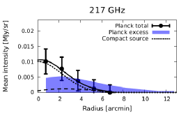
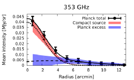
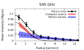
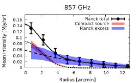
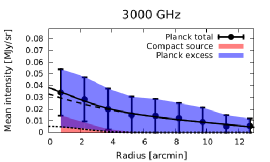
Figure 6: Radial profiles of the different components in the Planck and IRIS maps stacked at the positions of the SPT DSFGs. The panels show the azimuthally-averaged mean intensity, at each frequency, of: (a) the stacked map of the DSFGs (filled circles with error bars) – the cumulative flux densities obtained from this profile within a $3\hbox{\hbox to0.0pt{.\hss}\kern 0.80002pt}^{\scriptstyle\prime}\hbox{\kern-0.29999pt}5$ radius aperture are shown in Fig. 1 and in the black line in Fig. 3; (b) the compact source component after fitting a Gaussian profile with a FWHM that is fixed by the effective Planck (or IRIS, bottom panel) beam width ($1\sigma$ uncertainty, red shaded region); and (c) the excess obtained by removing the compact source component from the stack ($1\sigma$ uncertainty, blue shaded region). For each component of the stack, the uncertainties are derived from the bootstraps at each frequency. The short dashed line is a Gaussian fit (FWHM fixed by the beams) to the compact source profile. The long dashed line is a fit, using a cubic polynomial, to the mean intensity of the Planck (or IRIS, bottom panel) excess. The solid line is a sum of the fit to the compact source and the fit to the excess. At 217 GHz, since we have SPT flux density measurements for the full DSFG sample, we obtain the clustered component by fixing the normalization of the compact source component in the fit to the mean SPT flux density of the sample, as described in Sec. 4.1.

4.1.5 Components of the Planck stack: radial profiles

In Fig. 6, we show the azimuthally-averaged intensity profiles (centred at the position of the compact source) of: (1) the original stacked map; (2) the compact source after fitting to the source using the formalism in Appendix D; and (3) the Planck excess after removing the source from the stacked map. The aperture photometry flux densities we quote in this work (e.g., Fig. 1 and the black line in Fig. 3) are in fact the cumulative flux densities obtained by integrating profile (1) within a $3\hbox{\hbox to0.0pt{.\hss}\kern 0.80002pt}^{\scriptstyle\prime}\hbox{\kern-0.29999pt}5$ radius aperture. For each component of the stack, the uncertainties come from the bootstraps at each frequency.

If the excess emission measured by Planck is indeed associated with the SPT lensing halos at $z\sim 1$ that are along the line of sight to the high redshift compact source and if that excess emission originates from only the lensing halos, we would only detect this emission within the FWHM of the compact source profile (corresponding to a radius of $\sim 2.5\arcmin$ at 857 GHz). Instead, the radial profiles suggest that the excess emission is extended on a larger angular scale than that of the high redshift compact source. It follows that the excess emission would, in this case, also extend beyond the foreground lensing halo that is between the observer and the high redshift compact source. In particular, at 857 GHz, where we observe the largest magnitude of the excess emission (Fig. 4), we detect that emission out to a radius of 3.5$\arcmin$ from the compact source, at $2\sigma$ significance (beyond this radius, the significance of the detection decreases with increasing radius). This suggests that the excess emission could have a significant contribution from galaxies in neighbouring halos that surround the lensing halos. A theoretical prediction of the Planck excess should therefore take the contribution of these neighbouring halos into account (as we will do in Sec. 5).

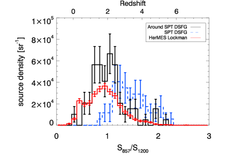
Figure 7: Resolving the excess with Herschel/SPIRE: Number density (within a $3\hbox{\hbox to0.0pt{.\hss}\kern 0.80002pt}^{\scriptstyle\prime}\hbox{\kern-0.29999pt}5$ radius from the position of the SPT DSFG) of detected sources by $S_{857}/S_{1200}$ colour bin. The sources considered are (a) sources detected at $S_{857}>50\thinspace{\rm mJy}$ around the SPT DSFGs (black); (b) all sources detected at $S_{857}>50\thinspace{\rm mJy}$ in the HerMES Lockman-SWIRE field (red); and (c) the SPT DSFGs themselves (blue). The horizontal axis on top shows the estimated redshift derived from the colours using a set of star-forming templates from Magdis et al. (2012) (it should be noted that this photometric redshift estimate is model-dependent).

4.2 The sources contributing to the Planck excess

We use the Herschel/SPIRE observations to probe the sources of the excess signal measured by Planck. The source detection and photometry are described in Sect. 3.2 and Appendix C. We first investigate if there is a statistical excess of such sources around the SPT DSFGs relative to a Poisson distribution of sources.

We focus on only high significance detections ($S_{857}>50\thinspace{\rm mJy}$), measuring the number densities of three types of sources: (1) $n_{\rm neighbours}$ for sources within $3\hbox{\hbox to0.0pt{.\hss}\kern 0.80002pt}^{\scriptstyle\prime}\hbox{\kern-0.29999pt}5$ of the DSFG; (2) $n_{\rm null}$ for sources detected at the same significance ($S_{857}>50\thinspace{\rm mJy}$) in the larger HerMES Lockman-SWIRE field; and (3) $n_{\rm DSFG}$ for the DSFGs themselves.

The computation of the source densities is described fully in Appendix G. In order to determine if such a clustering of sources is associated with the SPT DSFGs or with foreground structures along the line of sight to the DSFGs, we measure the variation of the number density of these three types of detected sources (DSFG neighbours, HerMES Lockman-SWIRE sources and the DSFGs themselves) as a function of their $S_{1200}/S_{857}$ colours. The result is shown in Fig. 7. The top horizontal axis of the same figure represents the photometric redshifts estimated from the sub-mm colours using the B12 effective template SEDs described in Sect. 4.1.3. We make the following observations:

• There is a significant excess of sources within $3\hbox{\hbox to0.0pt{.\hss}\kern 0.80002pt}^{\scriptstyle\prime}\hbox{\kern-0.29999pt}5$ of the DSFG, compared to the null test (using all other sources in the HerMES Lockman-SWIRE field which are detected at the same significance). The excess can also be expressed as the ratio of the mean density of the DSFG neighbours within $3\hbox{\hbox to0.0pt{.\hss}\kern 0.80002pt}^{\scriptstyle\prime}\hbox{\kern-0.29999pt}5$ of the DSFGs to the mean density of the sources in the entire HerMES Lockman-SWIRE field. We obtain a ratio of $2.18\pm 0.15$ at 1200 GHz and $1.76\pm 0.19$ at 857 GHz. The excess extends over a broad range of photometric redshifts from $z\sim 1$ to $z\sim 2$. This is consistent with the combined spectroscopic and photometric $n(z)$ for the lens galaxies. For the lens galaxies themselves, multi-wavelength imaging and spectroscopy has been obtained for more than 50 of the lensed SPT DSFGs (Rotermund et al., 2014). Spectroscopic redshifts are complete for $\sim 70\%$ of the sample, suggesting the median redshift of the lensing halos is at least $\langle z\rangle=0.6$, and with photometric redshifts for the remainder of the (optically fainter) sample, the median is close to the estimated SPT lens redshift of $z\sim 1$ in Hezaveh & Holder (2011).

• On average, the sources clustered around the SPT DSFGs are significantly bluer (in sub-mm colours) than the DSFGs themselves. Our SED fits suggest that these sources are at $z\sim 1-2$ whereas the DSFGs themselves are at $z>2$, consistent with $n(z)$ of the DSFG sample reported in Weiß et al. (2013).

We also estimate the mean colours of the three types of sources in Fig. 7. We compute the mean colour of the sources responsible for the Herschel excess $C_{\rm excess}$ according to:

$$C_{\rm excess}=\frac{\sum{C_{{\rm X},i}(N_{{\rm X},i}-N_{{\rm null},i})}}{\sum(N_{{\rm X},i}-N_{{\rm null},i})},$$ (1)

where $C_{{\rm X},i}$ is the $S_{857}/S_{1200}$ colour of the sources around the DSFG in each interval of colour $i$ in Fig. 7, $N_{{\rm X},i}$ is the number of such sources in that same colour interval, and $N_{{\rm null},i}$ is the number of HerMES Lockman-SWIRE sources in that same colour interval. The mean colours are $\langle S_{857}/S_{1200}\rangle=0.98\pm 0.01$ for the sources in the Lockman-SWIRE field, $\langle S_{857}/S_{1200}\rangle=1.10\pm 0.13$ for $C_{\rm excess}$ and $\langle S_{857}/S_{1200}\rangle=1.47\pm 0.05$ for the DSFGs. We check that cosmic variance has a negligible effect on the uncertainties in the number densities in each bin of colour in Fig. 7 by performing bootstrap realisations over the SPIRE fields around each SPT DSFG. The median ratio of the standard deviation in the number density over the bootstrap realisations to the Poisson uncertainty is 0.96. The mean colours are also dominated by the Poisson errors and not the cosmic variance. The sources responsible for the excess observed by Herschel thus have the same mean colour, and hence probably the same redshift, as the low redshift sources in HerMES Lockman-SWIRE. However, those sources clustered around the DSFGs are significantly bluer (by $\langle S_{857}/S_{1200}\rangle=0.4$ on average) compared to the DSFGs.

We also estimate a mean excess in flux density, $S_{\rm excess}$, of the detected sources around the DSFGs relative to all the other detected sources in the HerMES Lockman-SWIRE field, according to

$$S_{\rm excess}=\langle S_{\rm neighbours}\rangle-\langle S_{\rm null}\rangle,$$ (2)

where $\langle S_{\rm neighbours}\rangle$ is the mean flux density of the detected sources that are within $3\hbox{\hbox to0.0pt{.\hss}\kern 0.80002pt}^{\scriptstyle\prime}\hbox{\kern-0.29999pt}5$ of the SPT DSFGs and $\langle S_{\rm null}\rangle$ is the mean flux density of all the sources detected within an aperture of $3\hbox{\hbox to0.0pt{.\hss}\kern 0.80002pt}^{\scriptstyle\prime}\hbox{\kern-0.29999pt}5$ radius in the HerMES Lockman-SWIRE field, with:

$$\langle S_{\rm neighbours}\rangle=\frac{\sum{S_{\rm neighbours}}}{N_{\rm DSFG}},$$ (3)

where $N_{\rm DSFG}$ is the number of SPIRE maps of the SPT DSFGs (62 in practice, see Table 1) and

$$\langle S_{\rm null}\rangle=\frac{\sum{S_{\rm null}}\times\pi\times(3\hbox{\hbox to0.0pt{.\hss}\kern 0.80002pt}^{\scriptstyle\prime}\hbox{\kern-0.29999pt}5)^{2}}{A_{\rm L}},$$ (4)

where $A_{\rm L}$ is the total area of the Lockman-SWIRE field in square arcminutes.

We obtain $S_{\rm excess}$ of $130\pm 10$ mJy and $43\pm 5$ mJy at 1200 GHz and 857 GHz, respectively. It is important to note that the Herschel observations (with $S_{857}>50\thinspace{\rm mJy}$) thus recover approximately 20% of the Planck excess we measure at 857 GHz, and about 45% at 1200 GHz (see Fig. 4). If we assume $z=1.15$ for the lenses (Hezaveh & Holder, 2011), this resolved excess emission at 857 GHz translates into a mean $L_{\rm IR}$ of $(2.2\pm 0.2)\times 10^{12}\thinspace{\rm L}_{\mathord{\odot}}$ and a mean excess SFR of $(370\pm 40)\thinspace{\rm M}_{\mathord{\odot}}\thinspace{\rm yr}^{-1}$ per resolved source. This suggests that the environments around these massive $z\sim 1$ lensing halos host active star formation and that the galaxies in these environments that are responsible for this excess FIR emission are ultra-luminous infrared galaxies (ULIRGs).

To recover the full excess, we would require deeper imaging at a higher angular resolution (e.g., with ALMA). It is expected that Herschel detects this fraction of the extragalactic sources contributing to the CIB (Béthermin et al., 2012c) and the excess we measure with SPIRE (relative to random regions in the Universe) arises from bright, star-forming galaxies which are associated mainly with the foreground lensing halos of the SPT DSFGs. Finally, it should be noted that neither in the Planck nor Herschel analysis is it possible to pinpoint the sub-mm contribution from the lens galaxy itself. However, the lens galaxies are largely passive elliptical galaxies with no strong star formation (Hezaveh et al., 2013) and their contribution to $S_{\rm excess}$ is expected to be quite small.

5 Modeling the Planck excess

We have shown a large-scale excess of sub-mm emission that is detected out to a distance of $\sim 3.5\arcmin$ from the SPT DSFGs. We cannot interpret it as a classical clustering signal between the high redshift sources and their neighbours (Béthermin et al., 2010b, 2012c), because the colour of this excess indicates that the signal corresponds to objects at $z<2$ (see Sect. 4.1) whereas the SPT DSFGs lie mostly at $z\sim 2$–$6$ (Vieira et al., 2013; Weiß et al., 2013). However, both theoretical models (Negrello et al., 2007; Béthermin et al., 2011; Hezaveh & Holder, 2011) and observations (Vieira et al., 2013) predict that the large majority of bright SPT DSFGs are lensed. Consequently, there must be relatively massive dark matter halos along the line of sight to the SPT sources. Hezaveh & Holder (2011) predict a median mass of the lensing halos of $10^{13.3}\thinspace{\rm M}_{\mathord{\odot}}$. These massive halos are also strongly clustered (Mo & White, 1996; Sheth & Tormen, 1999; Sheth et al., 2001). The excess we measure with Planck could thus be the infrared emission coming mostly from galaxies which are in the neighbouring halos of the lenses.

The exact computation of the excess from a model of galaxy evolution that links the star formation process to the dark matter halos is beyond the scope of this paper. However, an estimate of the expected Planck excess can be performed with a more simplified computation. We use the halo model which assumes that all dark matter is bound in halos and provides a formalism for describing the clustering statistics of halos and galaxies (see Cooray & Sheth, 2002, and references therein). In this model, the one-halo term (due to distinct baryonic mass elements that lie within the same dark matter halo) dominates the correlation function on scales smaller than the virial radii of halos, while the two-halo term (due to baryonic mass elements in distinct pairs of halos) dominates the correlation function on larger scales. The halo occupation distribution (HOD, see Berlind et al., 2003) describes the clustering of galaxies within the halos – it is the probability that a halo of fixed virial mass hosts $N_{gal}$ galaxies. A standard approach to the HOD is to consider two populations of galaxies in the halos: central galaxies located at the centre of the host halo, and satellite galaxies distributed throughout the halo. In the context of the SPT lenses and their environments, the one-halo term thus takes into account the excess signal coming from the satellite galaxies within the lensing halo. The two-halo term accounts for the excess signal arising from clustering with galaxies in neighbouring halos. The use of the two-halo term is justified here because the Planck excess emission we observe extends out to $3\hbox{\hbox to0.0pt{.\hss}\kern 0.80002pt}^{\scriptstyle\prime}\hbox{\kern-0.29999pt}5$ from the DSFG, corresponding to a physical distance of 1.7 Mpc from the lensing halo at $z\sim 1$.

We start by computing the angular auto-correlation function $w_{\rm lens}(\theta)$ of $10^{13.3}\thinspace{\rm M}_{\mathord{\odot}}$ halos assuming the redshift distribution given by the Hezaveh & Holder (2011) model (median $z=1.15$, ${\rm FWHM}=1.53$). The computation is performed using the PMClib tools (Kilbinger et al., 2011; Coupon et al., 2012). We first estimate the two-halo term contribution by computing the HOD assuming no satellites. The cross-correlation function $\Psi$($\theta$) between the lensing halo and the halo hosting the neighbouring galaxies is then $\Psi(\theta)=b_{\rm CIB}/b_{\rm lens}\thinspace w_{\rm lens}(\theta)$, where $b_{\rm CIB}$ is the effective bias of sources responsible for the CIB, thus tracing galaxies in the neighbouring halos, and has a value of 2.4 at 857 GHz (Viero et al., 2009), $w_{\rm lens}(\theta)$ has a typical value of 0.029 at $\theta=5\arcmin$, and $b_{\rm lens}$ is the mean bias of the lensing halos. A mean bias of $b_{\rm lens}=3.6$ is used for the median halo mass at the median redshift of the lenses as predicted by Hezaveh & Holder (2011). The simple conversion above comes from the fact that $\Psi\propto b_{\rm CIB}\times b_{\rm lens}$ when $w_{\rm lens}\propto b_{\rm lens}^{2}$ (Cooray & Sheth, 2002), in the approximation that the redshift distributions of the two components are similar. This is a fair assumption here as Béthermin et al. (2012c) showed that the median redshift of the CIB at 857 GHz is 1.2.

From the auto-correlation function, we can compute the mean number excess, $e$, of infrared galaxies around the lensing halos:

$$e=\int_{\theta=0}^{3\hbox{\hbox to0.0pt{.\hss}\kern 0.56001pt}^{\scriptstyle\prime}\hbox{\kern-0.20999pt}5}\Psi(\theta)\theta d\theta.$$ (5)

We find an excess in the number density of galaxies of 2.3%. The total flux density of all galaxies at 857 GHz in a $3\hbox{\hbox to0.0pt{.\hss}\kern 0.80002pt}^{\scriptstyle\prime}\hbox{\kern-0.29999pt}5$ radius can be computed from the total contribution of galaxies to the CIB within this area, which is estimated in Béthermin et al. (2012c) to be 4300 mJy – the measured Planck excess at 857 GHz corresponds to 6$\%$ of this total contribution to the CIB within the same radius. The expected Planck signal from neighbouring halos (the 2-halo term) is thus $0.023\times 4300=99$ mJy.

Having computed the contribution from galaxies hosted by neighbouring halos of the lensing halos, we then compute the one-halo term contribution from galaxies inside the lensing halo itself, using a different formalism. We assume a standard halo-mass-to-infrared-light ratio estimated from abundance matching (Béthermin et al., 2012b, a) and the satellite mass function of Tinker & Wetzel (2010). By contrast with the two-halo term computation, here we consider both central and satellite galaxies in the lensing halo. For a halo of $10^{13.3}\thinspace{\rm M}_{\mathord{\odot}}$ at $z=1.15$, we find a total flux density from the central and satellite galaxies in the lensing halo of 20 mJy. These predictions are upper limits because the model neglects the environmental quenching of satellites around massive galaxies. The total expected contribution of both the one-halo and two-halo terms is thus 119 mJy at 857 GHz. The prediction from this relatively simple model is in broad agreement with the Planck measurement of the excess ($210\pm 78$ mJy at 857 GHz). In fact, there is a weak indication that the measured value is higher than the model prediction, due to, perhaps, enhanced star formation that could originate from the dense environments around the lensing halos, but the Planck signal does not have sufficient signal-to-noise to confirm this. Finally, we also determine how sensitive the predicted amplitude of the emission is to the assumed halo mass. We obtain 50 mJy (one-halo term) and 148 mJy (two-halo term) for a halo mass of $10^{13.8}\thinspace{\rm M}_{\mathord{\odot}}$, giving a total predicted excess of 200 mJy for $10^{13.8}\thinspace{\rm M}_{\mathord{\odot}}$ halos. We obtain 8 mJy (one-halo term) and 70 mJy (two-halo term) for a halo mass of $10^{12.8}\thinspace{\rm M}_{\mathord{\odot}}$, giving a total predicted excess of 80 mJy for $10^{12.8}\thinspace{\rm M}_{\mathord{\odot}}$ halos.

6 Discussion

Our results support the picture of active star formation proceeding in dense environments at $z\sim 1$. Using a simple model that connects star formation to dark matter halos, we predict that most of this excess emission (around $80\%$) that is detected by Planck should arise from galaxies in the neighboring halos of the foreground lensing halos (the two-halo term in the context of the halo model). A proportion of the excess emission measured by Planck ($20\%$ at 857 GHz and $45\%$ at 1200 GHz) is associated with individual sources detected by Herschel. The sources that contribute to this resolved excess are consistent with being ULIRGs ($L_{\rm IR}>10^{12}\thinspace{\rm L}_{\mathord{\odot}}$). The remainder of the excess FIR emission measured by Planck which is not resolved by Herschel must therefore come from an excess of fainter infrared galaxies ($L_{\rm IR}<10^{12}\thinspace{\rm L}_{\mathord{\odot}}$) at $z\sim 1$ that are in these dense environments.

Several studies (e.g., Noble et al., 2012) report an excess in the number densities of sub-mm galaxies in mass-biased regions of the $z\gtrsim 1$ Universe, relative to blank fields. Although the number statistics are low, surveys towards $z\sim 1$ clusters (e.g., Best, 2002; Webb et al., 2005) suggest that the optical Butcher–-Oemler effect (where a population of blue, star-forming galaxies appears in many $z>0.3$ clusters) is also observed at sub-mm wavelengths. These studies also suggest that if the DSFGs responsible for this excess are confirmed to be at the same redshift as the $z\sim 1$ clusters, their SFRs would be consistent with those of ULIRGs.

Our results are qualitatively consistent with other studies that find active star formation proceeding in dense environments at $z$$\sim$$1$. Brodwin et al. (2013) investigated star-forming properties of galaxy clusters at $1<z<1.5$ and found extensive star formation increasing toward the centres of clusters. Alberts et al. (2014) showed that the SFR in clusters grows more rapidly with increasing redshift than it does in the field, and surpasses the field values around $z\sim 1.4$. Feruglio et al. (2010) found that although the ULIRG$+$LIRG fraction decreases with increasing galaxy density up to $z$$\sim$$1$, the dependence on density flattens from $z=0.4$ to $z=1$. They observed that a large fraction of highly star-forming LIRGs is still present in the most dense environments at $z$$\sim$$1$. The dense environments at $z$$\sim$$1$, including those associated with the SPT lensing halos that we probe in this study, may well be the progenitors of the massive galaxies found in the centres of clusters at $z\sim 0$.

An optical follow-up study of the lens environments will investigate the LIRG hypothesis in more detail. Rotermund et al. (2014) have already used spectroscopic and photometric studies to constrain the $N(z)$ of the SPT lensing halos ($\langle z\rangle>0.6$), and have studied the relative overdensities surrounding the lensing galaxies. However, an analysis of star forming galaxies in these environments has yet to be carried out. Finally, we note that the Planck survey itself will be able to find overdensities at $z\gtrsim 2$ across the full sub-mm sky by selecting the coldest fluctuations of the CIB (Dole et al., 2014).

7 Conclusions

We stack Planck HFI maps at the locations of DSFGs identified in SPT data. The stack provides an ensemble average of the flux density of the background DSFGs, the foreground lensing halos at $z\sim 1$, and the surrounding environments. Though the SPT DSFGs lie at much higher redshift ($z\sim 2-6$), they are angularly correlated with massive ($\sim 10^{13}{\rm M}_{\mathord{\odot}}$) dark matter halos at $z\sim 1$ through strong gravitational lensing. We isolate a clustered component which extends to large angular scales in the stack and demonstrate that it originates from sub-mm emission from star formation in these environments. We exploit Planck’s wide frequency coverage to estimate a photometric redshift for the clustered component from the far-infrared colours. We then use higher resolution Herschel/SPIRE observations in order to study the sources in these dense environments that contribute to the clustering signal. Our results can be summarized as follows.

• We find a mean excess of star formation rate (SFR) compared to the field, of $(2700\pm 700)\thinspace{\rm M}_{\mathord{\odot}}\thinspace{\rm yr}^{-1}$ from all galaxies contributing to the clustering signal within a radius of $3\hbox{\hbox to0.0pt{.\hss}\kern 0.80002pt}^{\scriptstyle\prime}\hbox{\kern-0.29999pt}5$ from the positions of the SPT DSFGs. The sources responsible for the clustering signal are galaxies clustered within about $2$ Mpc around the foreground lensing halo at $z\sim 1$. The magnitude of the measured Planck excess due to the clustered component ($210\pm 78$ mJy at 857 GHz) broadly agrees with the prediction of a model of the CIB that links infrared luminosities with dark matter halos. The measured excess at 857 GHz corresponds to approximately $5\%$ of the total contribution of all galaxies to the CIB within a $3\hbox{\hbox to0.0pt{.\hss}\kern 0.80002pt}^{\scriptstyle\prime}\hbox{\kern-0.29999pt}5$ radius. The model predicts that the excess emission (and hence star formation) should be dominated (around $80\%$) by the two-halo term contribution, due to galaxies in the neighbouring halos which are clustered around the lensing halo itself.

• A fraction (approximately $20\%$ at 857 GHz with $S_{857}>50$ mJy) of the excess emission from these dense $z\sim 1$ environments is resolved by Herschel. The sources contributing to this resolved excess are highly star-forming ULIRGs ($L\sim 10^{12.5}\thinspace{\rm L}_{\mathord{\odot}}$). The mean excess of SFR, relative to the field, due to these detected sources is $370\pm 40\thinspace{\rm M}_{\mathord{\odot}}\thinspace{\rm yr}^{-1}$ per resolved source. The remainder of excess star formation could originate from fainter LIRGs that are in highly dense regions within the neighbouring halos. The overall picture therefore suggests that these dense environments at $z\sim 1$ are still actively forming stars. This is qualitatively consistent with the SFR-density relation reversing at $z\sim 1$ when compared to $z\sim 0$.

• Our work shows that in an experiment where the beam FWHM is comparable or larger than the angular scale of the clustering signal, the stacked flux density estimates of high redshift lensed DSFGs will have significant contributions from galaxies clustered around the lensing halos that are along the line-of-sight to the background lensed galaxies. The relative clustering contamination has a clear dependence on frequency: in Planck data, we measure it to be 0.1$\pm$0.6 at 217 GHz, 0.2$\pm$0.2 at 353 GHz, 0.5$\pm$0.2 at 545 GHz, and 1.1$\pm$0.4 at 857 GHz. This contamination should be taken into account in order to obtain the correct flux densities of the background galaxies with Planck data.

Appendix A Uncertainties in the Planck and IRIS stacked maps of the DSFGs

Table 3: Uncertainties in the stacked Planck (at $217-857$ GHz) and IRIS (at 3000 GHz) maps which are co-added at the locations of the SPT DSFGs: (1) photometric uncertainties $\sigma_{phot}$ estimated from the standard deviation of flux densities over 1000 iterations of stacking 65 randomly chosen patches in the sky (dashed lines in Fig 1); and (2) bootstrap uncertainties $\sigma_{\rm boot}$ computed from the standard deviation of flux densities over 1000 bootstrap realizations of the stacked maps of the 65 DSFGs (solid lines in Fig 1). The sample heterogeneity $\sigma_{\rm pop}$ is the intrinsic dispersion in the DSFG population. It is estimated at each Planck frequency by extrapolating the flux density dispersion at the SPT frequency to the Planck frequencies. $S_{\nu}$ is the mean flux density from performing aperture photometry on the bootstrap realizations of the stacked maps of the DSFGs, and $S_{\nu,compact}$ is the mean flux density of the compact source component in the stack.

Type of variance	217 GHz	353 GHz	545 GHz	857 GHz	3000 GHz
$\sigma_{\rm phot}$ [mJy]	13$\pm$0.4	13$\pm$0.4	30$\pm$0.9	75$\pm$2.4	106$\pm$3.4
$\sigma_{\rm phot}/S_{\nu}$	0.40	0.11	0.11	0.19	0.87
$\sigma_{\rm pop}$ [mJy]	1.5	5.4	8.9	10.0	0.6
$\sigma_{\rm pop}/S_{\nu,compact}$	0.05	0.05	0.05	0.05	0.05
$\sqrt{\sigma_{\rm phot}^{2}+\sigma_{\rm pop}^{2}}$	13	14	31	76	106
$\sigma_{\rm boot}$ [mJy]	16$\pm$2	16$\pm$2	31$\pm$4	73$\pm$10	85$\pm$11
$\sigma_{\rm boot}/S_{\nu}$	0.51	0.13	0.12	0.18	0.67

In Table 3, we compare the uncertainties from bootstrapping, $\sigma_{\rm boot}$, with the photometric uncertainties, $\sigma_{\rm phot}$, derived from performing aperture photometry in the random patches of the SPT fields. In order to compare how close $\sigma_{\rm boot}$ and $\sigma_{\rm phot}$ are to each other, we also compute an uncertainty on them – these scale as $1/\sqrt{(}N_{sources})$ for $\sigma_{\rm boot}$ and $1/\sqrt{(}N_{iter})$ for $\sigma_{\rm phot}$, where $N_{sources}$ is the number of sources in the stack (65) and $N_{iter}$ is the number of stacking iterations (1000). $\sigma_{\rm phot}$ includes both the instrumental and confusion noise. We estimate the standard deviation of the average flux density of the stacked population, $\sigma_{\rm pop}$ assuming that the relative scatter on the flux density of the SPT sources does not depend on wavelength:

$$\sigma_{\rm pop}=\frac{\sigma_{\rm 220}}{\sqrt{N_{sources}}}\times\frac{S_{\nu,compact}}{S_{\rm 220}}$$ (6)

where $S_{\rm 220}$ is the mean flux density of the DSFG sample measured by SPT at 220 GHz, $\sigma_{\rm 220}$ is the standard deviation of the SPT flux densities (sources detected individually) and $S_{\rm\nu,compact}$ is the mean flux density of the compact source component in the stack. Table 3 shows that the bootstrap uncertainties are very close to the photometric uncertainties at 217$-$857 GHz. The bootstrap uncertainties combine the photometric noise and the heterogeneity of the population (Béthermin et al., 2012c):

$$\sigma_{\rm boot}=\sqrt{\sigma_{\rm phot}^{2}+\sigma_{\rm pop}^{2}}$$ (7)

Table 3 shows that this intrinsic dispersion as characterized by $\sigma_{\rm pop}$ is very small compared to the photometric uncertainties. At 3000 GHz, $\sigma_{\rm phot}$ is somewhat higher than $\sigma_{\rm boot}$ (although still within $2\sigma$) due to possible complex effects of Galactic cirrus. In general, the 353, 545 and 857 GHz channels are cleaner than the 3000 and 217 GHz channels and allow better constraints on the properties of the DSFGs.

Appendix B Determining the effect of pixelisation on the FWHM in the HEALPix maps

The Planck HFI maps are pixelized using the HEALPix scheme at resolution $N_{\mathrm{grid}}=2048$, corresponding to $5\times 10^{7}$ pixels over the full sky. This pixelation can lead to positional offsets as large as $0\hbox{\hbox to0.0pt{.\hss}\kern 0.80002pt}^{\scriptstyle\prime}\hbox{\kern-0.29999pt}5$ and can enlarge the effective beam. We calculate the magnitude of this effect using simulations of the stacking analysis. Since the offsets depend on the sky position, we begin by inserting simulated sources with the measured Planck beam (Planck Collaboration VII, 2014) at the known source locations. We then extract $1^{\circ}\times 1^{\circ}$ maps centred at each source location, stack these maps, and measure the beam FWHM in the stacked map. The final FWHMs are $4\hbox{\hbox to0.0pt{.\hss}\kern 0.80002pt}^{\scriptstyle\prime}\hbox{\kern-0.29999pt}64$, $4\hbox{\hbox to0.0pt{.\hss}\kern 0.80002pt}^{\scriptstyle\prime}\hbox{\kern-0.29999pt}97$, $5\hbox{\hbox to0.0pt{.\hss}\kern 0.80002pt}^{\scriptstyle\prime}\hbox{\kern-0.29999pt}10$, and $5\hbox{\hbox to0.0pt{.\hss}\kern 0.80002pt}^{\scriptstyle\prime}\hbox{\kern-0.29999pt}30$ for the Planck 857, 545, 353, and 217 GHz bands respectively, and $4\hbox{\hbox to0.0pt{.\hss}\kern 0.80002pt}^{\scriptstyle\prime}\hbox{\kern-0.29999pt}61$ for the IRIS 3000 GHz band.

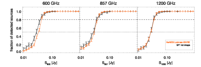
Figure 8: Monte Carlo simulations with sources injected into the 10$\arcmin\times$10$\arcmin$ SPIRE maps of SPT DSFGs at 600, 857, and 1200 GHz. Top panel: ratio of output to input flux densities as a function of the input flux density at the each frequency. Bottom panel: fraction of recovered sources as a function of the input flux density of the sources at each frequency. This is plotted for: (a) the maps containing the SPT sources (black); (b) sources in the entire HerMES Lockman SWIRE field (orange).

Appendix C Monte Carlo simulations on Herschel maps

We perform Monte Carlo simulations to test the robustness of the source detection and photometry in both the $10\arcmin\times 10\arcmin$ SPIRE maps of the SPT DSFGs and the larger HerMES Lockman-SWIRE field. We inject sources of known flux densities at random positions into the maps. We inject 5 sources of a given flux density into each $10^{\circ}\times 10^{\circ}$ map, and record the fraction of sources that are detected. This process is repeated for source flux densities from 10 to 1000 mJy. The same process is applied to the larger HerMES Lockman-SWIRE field, however the number of sources is increased to 1000. Fig. 8 shows: (1) a comparison of the input and output flux densities and (2) the completeness, defined as the fraction of recovered sources, as a function of the input flux densities, for both the SPIRE maps of the SPT DSFGs and the HerMES Lockman-SWIRE field. The simulations for completeness show that the fraction of injected sources that are recovered becomes $\gtrsim 0.8$ at flux densities above around $50$ mJy for both the 1200 and 857 GHz bands.

Appendix D Formalism to measure the flux density of the DSFG and excess in the stacked Planck maps

We use the formalism of Béthermin et al. (2010a) to disentangle source and clustering contributions to the total flux within the Planck beam. Béthermin et al. (2012c) used this method to estimate the level of contamination due to clustering in the deep number counts at 1200, 857 and 600 GHz in HerMES. They fitted stacked images of the SPIRE sources with an auto-correlation function (ACF) $w(\theta)$ which is convolved with the beam function. Heinis et al. (2013) have also applied this method to UV stacking. In particular:

• We fit the compact source component with a 2-dimensional Gaussian profile whose width is determined by the PSF FWHM of the Planck beams as described in Appendix B.

• We fit the clustered component around the source using an angular correlation function $w(\theta)\propto{\theta}^{-0.8}$ that is first convolved with the Planck PSF FWHM at each frequency (the exponent comes from measurements of the angular correlation function of galaxies, e.g., Baugh et al., 1996; Connolly et al., 1998).

• We assume a constant background level.

We define the quantity $s^{2}$ as the difference between the fluxes of the raw stacked Planck maps and a linear combination of the above 3 profiles that are fitted to the stacked map $m_{i{,}j}$:

$$s^{2}=\sum_{i{,}j}{(m_{ij}-\alpha p_{ij}+\beta c_{ij}+\gamma\times\textbf{1}_{ij})^{2}},$$ (8)

where $p_{ij}$ is an array containing the PSF in 2 dimensions ($i{,}j$); $c_{ij}$ is an array containing the clustering signal and $\textbf{{1}}_{ij}$ is an array containing only 1s and represents the background (assumed to be constant). The sum runs over all the pixels $N_{\rm pix}$ in the map. The quantities $\alpha$, $\beta$ and $\gamma$ are normalisation constants for the flux density of the compact source component, clustered component and the background component, respectively. Minimizing $s^{2}$ with respect to $\alpha,\beta$ and $\gamma$ leads to a simple matrix equation

$$\mn@boldsymbol{c}=\textbf{{A}}\thinspace\mn@boldsymbol{b},$$ (9)

where A is defined as:

$$\textbf{{A}}=\left(\begin{array}[]{ccc}\sum_{i,j}{p_{ij}^{2}}&\sum_{i,j}{p_{ij}c_{ij}}&\sum_{i,j}{p_{ij}}\\ \sum_{i,j}{p_{ij}c_{ij}}&\sum_{i,j}{c_{ij}^{2}}&\sum_{i,j}{c_{ij}}\\ \sum_{i,j}{p_{ij}}&\sum_{i,j}{c_{ij}}&N_{\rm pix}\end{array}\right)\thinspace,$$ (10)

with $\mn@boldsymbol{b}$ defined as:

$$\mn@boldsymbol{b}=\left(\begin{array}[]{c}\alpha\\ \beta\\ \gamma\end{array}\right)\thinspace,$$ (11)

and $\mn@boldsymbol{c}$ defined as:

$$\mn@boldsymbol{c}=\left(\begin{array}[]{c}\sum_{i,j}{m_{ij}p_{ij}}\\ \sum_{i,j}{m_{ij}c_{ij}}\\ \sum_{i,j}{m_{ij}}\end{array}\right).$$ (12)

By inverting A and solving this equation, we obtain flux densities of each component $\alpha$, $\beta$, and $\gamma$.

Appendix E Tests of the Planck clustered component

E.1 Stacking simulations

We generate 1000 realisations of 65 $1^{\circ}\times 1^{\circ}$ maps (the same number as in the SPT DSFG sample) where each map contains a compact source component (which is at the centre of the map and modeled as a Gaussian with a FWHM given by the Planck beams) and a clustered component, according to the model given in Appendix D. The input flux densities of the two components are chosen to match the measured mean flux densities given in Table 2. In each individual simulated map, the source and clustering components are added to one of the randomly chosen blank maps in the Planck sky (discussed in Sect 3.1 and in Figure 1). For each of 1000 realisations of the stacked maps, we measure the total flux density within a 3.5$\arcmin$ radius of the central compact source using aperture photometry, and we compare this flux density to the total input flux density at each frequency. We also apply the formalism in Appendix D to each realisation of the stacked maps in order to recover the flux densites of the compact source component and the clustered component at each frequency, and we compare these with their input flux densities. In Table 4, we report the difference between the recovered mean flux density (over 1000 realisations) and the input flux density at each frequency, as a fraction of the statistical uncertainty (given by the photometric uncertainty $\sigma_{phot}$ in each stacked map).

Table 4: The systematic bias, arising from the stacking procedure, in the measured flux density of the high redshift compact component and the clustering component (obtained from the fitting method in Appendix D) and in the measured total flux density (obtained from aperture photometry). Artificial compact source components and clustered components are injected into blank Planck and IRIS maps before these maps are stacked (see Appendix E.1 for details). The difference between the mean recovered flux density of each component (over 1000 stacking realisations) and their true flux density at each frequency is expressed in terms of the photometric uncertainties $\sigma_{phot}$ in the stacked maps.

Frequency	217 GHz	353 GHz	545 GHz	857 GHz	3000 GHz
Systematic bias in mean flux density of all components (from aperture photometry)	0.31$\sigma$	0.38$\sigma$	0.39$\sigma$	0.33$\sigma$	0.19$\sigma$
Systematic bias in mean flux density of compact source component (from fit)	0.01$\sigma$	0.23$\sigma$	0.25$\sigma$	0.16$\sigma$	0.05$\sigma$
Systematic bias in mean flux density of clustered component (from fit)	0.31$\sigma$	0.13$\sigma$	0.07$\sigma$	0.16$\sigma$	0.20$\sigma$

Figure 9: Six realisations of Planck and IRIS residual maps (in units of MJy$sr^{-1}$) after introducing a random rotation of 90^∘ in individual maps of the SPT DSFGs before stacking the maps at the positions of the SPT DSFGs, and then removing the central compact source component in each realisation of the stacked maps using the formalism in Appendix D. The original size of the stacked maps is $1^{\circ}\times 1^{\circ}$. Here, we show the $10\arcmin\times 10\arcmin$ central region in order to see the residual structure more clearly.

Figure 10: Top panel: Planck and IRIS maps (in units of MJy$sr^{-1}$) stacked at the positions of 65 SPT synchrotron sources (Vieira et al., 2010). Each map in the stack is centred on the SPT-derived position of the synchrotron source. The original size of the stacked maps is $1^{\circ}\times 1^{\circ}$. Here, we show the central $20\arcmin\times 20\arcmin$ region in order to see the residual structure more clearly. Bottom panel: residual maps after the compact source (the SPT synchrotron source) at the centre of the stacked maps is removed using the formalism in Appendix D.

E.2 Random rotations of maps

We make another 1000 realisations of stacking Planck and IRIS maps at the positions of the SPT DSFGs by rotating the individual maps randomly by 90^∘ before stacking them. In each realisation, we then remove the compact source component from the stacked map at each frequency using the formalism in Appendix D. Six realisations of the residual maps which are obtained after the removal of the compact source are chosen at random and displayed in Figure 9. We also verified that the measured mean flux densities in this work did not change significantly when we introduced the random rotations of the individual maps.

E.3 Stacking maps of SPT synchrotron sources

We stack Planck and IRIS maps at the positions of a sample of 65 synchrotron sources detected in the SPT survey (Vieira et al., 2010) and with $S_{220}>20$ mJy. These sources are not angularly correlated with foreground structure, unlike the SPT DSFGs. We then remove the compact source component from the stacked maps at each frequency using the formalism in Appendix D. The results are shown in Figure 10. We observe no significant excess emission at 217$-$857 GHz after removal of the central compact source. The residual maps are very different to those for the SPT DSFGs (Fig 2) where we observe a clear extended emission at 545 and 857 GHz.

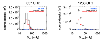
Figure 11: Number density of detected sources as a function of their flux densities at 857 GHz (left) and 1200 GHz (right). The sources considered are: (a) those detected at $S_{857}>50$ mJy around the DSFG (black); (b) all sources detected at $S_{857}>50$ mJy in the HerMES Lockman-SWIRE field (red); and (c) the SPT DSFG themselves (blue). This figure is analogous to Fig. 7, which shows the number density of the detected sources (of each of the 3 types) by their $S_{857}/S_{1200}$ colour.

Appendix F Determining $p(z)$ of the compact source and Planck excess from the stack

In order to obtain the probability distribution for the redshift $p(z)$ for both the compact source component and the Planck excess signal, the expected flux density, $T_{i}$, for each frequency channel, $i$, is calculated for the template SEDs at a range of redshifts $z\in[0,6]$. A $\chi^{2}$ value is computed for each $z$:

$$\chi^{2}(z)=\sum_{i=0}^{N_{\rm f}}{\frac{(F_{i}-b(z)T_{i}(z))^{2}}{\sigma_{i}^{2}}},$$ (13)

where $F_{i}$ is the observed flux density through channel $i$, $\sigma_{i}$ is the error in $F_{i}$, $T_{i}(z)$ is the flux density in the same channel for the template SED at redshift $z$, $N_{\rm f}$ is the number of frequency channels, and $b(z)$ is a scaling factor that normalizes the template to the observed flux density and is determined by minimizing Eq. 13 with respect to $b$ at that redshift, giving

$$b(z)=\frac{\sum_{i=0}^{N_{\rm f}}F_{i}T_{i}(z)/\sigma_{i}^{2}}{\sum_{i=0}^{N_{\rm f}}T_{i}(z)^{2}/\sigma_{i}^{2}}.$$ (14)

The probability distribution for the redshift, $p(z)$, will have the form:

$$p(z)\propto e^{-{\chi^{2}(z)}}.$$ (15)

Appendix G Measuring number densities in Herschel

We estimate the number densities for the three different types of sources as follows.

• The number density (per ${\rm sr}^{-1}$), $n_{\rm neighbours}$, of sources with $S_{857}>50$ mJy within $3\hbox{\hbox to0.0pt{.\hss}\kern 0.80002pt}^{\scriptstyle\prime}\hbox{\kern-0.29999pt}5$ of the DSFGs, defined by:

  $$n_{\rm neighbours}=\frac{N_{\rm sources}}{N_{\rm DSFG}\times\omega_{\rm aper}}$$ (16)

  , where $N_{\rm sources}$ is the number of detected sources around the DSFG, $N_{\rm DSFG}$ is the number of apertures, and $\omega_{\rm aper}$ is the solid angle subtended by the aperture. The DSFG is not counted in $N_{\rm sources}$.

• The number density, $n_{\rm null}$, of all sources with $S_{857}>50$ mJy across the entire HerMES Lockman-SWIRE field. We will use this as a null test.

• The number density of SPT DSFGs, $n_{\rm DSFG}$, with $S_{220}>20$ mJy using the same SPIRE maps of the SPT DSFGs.

Figure 11 shows the number density of the detected sources (for each of the above three classes) per bin of flux density at 1200 and 857 GHz. Throughout this paper, we use $S_{220}>20$ mJy for the SPT flux selection.

References

- Alberts et al. (2014) Alberts S. et al., 2014, MNRAS, 437, 437
- Baugh et al. (1996) Baugh C. M., Gardner J. P., Frenk C. S., Sharples R. M., 1996, MNRAS, 283, L15
- Benson et al. (2000) Benson A. J., Cole S., Frenk C. S., Baugh C. M., Lacey C. G., 2000, MNRAS, 311, 793
- Berlind et al. (2003) Berlind A. A. et al., 2003, ApJ, 593, 1
- Berta et al. (2011) Berta S. et al., 2011, A&A, 532, A49
- Best (2002) Best P. N., 2002, MNRAS, 336, 1293
- Béthermin et al. (2012a) Béthermin M. et al., 2012a, ApJ, 757, L23
- Béthermin et al. (2010a) Béthermin M., Dole H., Beelen A., Aussel H., 2010a, A&A, 512, A78
- Béthermin et al. (2010b) Béthermin M., Dole H., Cousin M., Bavouzet N., 2010b, A&A, 516, A43
- Béthermin et al. (2011) Béthermin M., Dole H., Lagache G., Le Borgne D., Penin A., 2011, A&A, 529, A4
- Béthermin et al. (2012b) Béthermin M., Doré O., Lagache G., 2012b, A&A, 537, L5
- Béthermin et al. (2012c) Béthermin M. et al., 2012c, ArXiv e-prints
- Blain et al. (2002) Blain A. W., Smail I., Ivison R. J., Kneib J.-P., Frayer D. T., 2002, Phys. Rep., 369, 111
- Blake et al. (2006) Blake C., Pope A., Scott D., Mobasher B., 2006, MNRAS, 368, 732
- Blanton et al. (2005) Blanton M. R., Eisenstein D., Hogg D. W., Schlegel D. J., Brinkmann J., 2005, ApJ, 629, 143
- Bourne et al. (2012) Bourne N. et al., 2012, MNRAS, 421, 3027
- Brodwin et al. (2013) Brodwin M. et al., 2013, ApJ, 779, 138
- Carlstrom et al. (2011) Carlstrom J. E. et al., 2011, PASP, 123, 568
- Connolly et al. (1998) Connolly A. J., Szalay A. S., Brunner R. J., 1998, ApJ, 499, L125
- Cooper et al. (2008) Cooper M. C. et al., 2008, MNRAS, 383, 1058
- Cooray & Sheth (2002) Cooray A., Sheth R., 2002, Phys. Rep., 372, 1
- Coupon et al. (2012) Coupon J. et al., 2012, A&A, 542, A5
- Diolaiti et al. (2000) Diolaiti E., Bendinelli O., Bonaccini D., Close L., Currie D., Parmeggiani G., 2000, in Astronomical Society of the Pacific Conference Series, Vol. 216, Astronomical Data Analysis Software and Systems IX, Manset N., Veillet C., Crabtree D., eds., p. 623
- Dole et al. (2006) Dole H. et al., 2006, A&A, 451, 417
- Dole et al. (2014) Dole et al., 2014, in prep.
- Elbaz et al. (2007) Elbaz D. et al., 2007, A&A, 468, 33
- Fernandez-Conde et al. (2008) Fernandez-Conde N., Lagache G., Puget J.-L., Dole H., 2008, A&A, 481, 885
- Fernandez-Conde et al. (2010) Fernandez-Conde N., Lagache G., Puget J.-L., Dole H., 2010, A&A, 515, A48
- Feruglio et al. (2010) Feruglio C. et al., 2010, ApJ, 721, 607
- Górski et al. (2005) Górski K. M., Hivon E., Banday A. J., Wandelt B. D., Hansen F. K., Reinecke M., Bartelmann M., 2005, ApJ, 622, 759
- Greve et al. (2012) Greve T. R. et al., 2012, ApJ, 756, 101
- Griffin et al. (2010) Griffin M. J. et al., 2010, A&A, 518, L3
- Heinis et al. (2013) Heinis S. et al., 2013, MNRAS, 429, 1113
- Hezaveh & Holder (2011) Hezaveh Y. D., Holder G. P., 2011, ApJ, 734, 52
- Hezaveh et al. (2013) Hezaveh Y. D. et al., 2013, ApJ, 767, 132
- Hildebrandt et al. (2013) Hildebrandt H. et al., 2013, MNRAS, 429, 3230
- Hogg et al. (2004) Hogg D. W. et al., 2004, ApJ, 601, L29
- Holder et al. (2013) Holder G. P. et al., 2013, ApJ, 771, L16
- Hwang et al. (2010) Hwang H. S. et al., 2010, MNRAS, 409, 75
- Kennicutt (1998) Kennicutt, Jr. R. C., 1998, ApJ, 498, 541
- Kilbinger et al. (2011) Kilbinger M. et al., 2011, ArXiv e-prints
- Kurczynski & Gawiser (2010) Kurczynski P., Gawiser E., 2010, AJ, 139, 1592
- Lagache et al. (2005) Lagache G., Puget J.-L., Dole H., 2005, ARA&A, 43, 727
- Lamarre et al. (2010) Lamarre J. et al., 2010, A&A, 520, A9
- Magdis et al. (2012) Magdis G. E. et al., 2012, ApJ, 760, 6
- Magnelli et al. (2010) Magnelli B. et al., 2010, A&A, 518, L28
- Miville-Deschênes & Lagache (2005) Miville-Deschênes M.-A., Lagache G., 2005, ApJS, 157, 302
- Mo & White (1996) Mo H. J., White S. D. M., 1996, MNRAS, 282, 347
- Mocanu et al. (2013) Mocanu L. M. et al., 2013, ArXiv e-prints
- Moshir et al. (1992) Moshir M., Kopman G., Conrow T. A. O., 1992, IRAS Faint Source Survey, Explanatory supplement version 2
- Negrello et al. (2007) Negrello M., Perrotta F., González-Nuevo J., Silva L., de Zotti G., Granato G. L., Baccigalupi C., Danese L., 2007, MNRAS, 377, 1557
- Neugebauer et al. (1984) Neugebauer G. et al., 1984, ApJ, 278, L1
- Nguyen et al. (2010) Nguyen H. T. et al., 2010, A&A, 518, L5
- Noble et al. (2012) Noble A. G. et al., 2012, MNRAS, 419, 1983
- Oliver et al. (2012) Oliver S. J. et al., 2012, MNRAS, 424, 1614
- Planck Collaboration I (2011) Planck Collaboration I, 2011, A&A, 536, A1
- Planck Collaboration I (2014) Planck Collaboration I, 2014, A&A, in press, [arXiv:astro-ph/1303.5062]
- Planck Collaboration IX (2014) Planck Collaboration IX, 2014, A&A, in press, [arXiv:astro-ph/1303.5070]
- Planck Collaboration VI (2014) Planck Collaboration VI, 2014, A&A, in press, [arXiv:astro-ph/1303.5067]
- Planck Collaboration VII (2014) Planck Collaboration VII, 2014, A&A, in press, [arXiv:astro-ph/1303.5068]
- Planck Collaboration XVIII (2011) Planck Collaboration XVIII, 2011, A&A, 536, A18
- Planck Collaboration XVIII (2014) Planck Collaboration XVIII, 2014, A&A, in press, [arXiv:astro-ph/1303.5078]
- Planck HFI Core Team (2011) Planck HFI Core Team, 2011, A&A, 536, A4
- Popesso et al. (2011) Popesso P. et al., 2011, A&A, 532, A145
- Reichardt et al. (2012) Reichardt C. L. et al., 2012, ApJ, 755, 70
- Rotermund et al. (2014) Rotermund et al., 2014, in prep.
- Schlegel et al. (1998) Schlegel D. J., Finkbeiner D. P., Davis M., 1998, ApJ, 500, 525
- Sheth et al. (2001) Sheth R. K., Mo H. J., Tormen G., 2001, MNRAS, 323, 1
- Sheth & Tormen (1999) Sheth R. K., Tormen G., 1999, MNRAS, 308, 119
- Siringo et al. (2009) Siringo G. et al., 2009, A&A, 497, 945
- Story et al. (2013) Story K. T. et al., 2013, ApJ, 779, 86
- Swinyard et al. (2010) Swinyard B. M. et al., 2010, A&A, 518, L4
- Tauber et al. (2010) Tauber J. A. et al., 2010, A&A, 520, A1
- Tinker & Wetzel (2010) Tinker J. L., Wetzel A. R., 2010, ApJ, 719, 88
- Vieira et al. (2010) Vieira J. D. et al., 2010, ApJ, 719, 763
- Vieira et al. (2013) Vieira J. D. et al., 2013, Nature, 495, 344
- Viero et al. (2009) Viero M. P. et al., 2009, ApJ, 707, 1766
- Viero et al. (2013a) Viero M. P. et al., 2013a, ApJ, 779, 32
- Viero et al. (2013b) Viero M. P. et al., 2013b, ApJ, 772, 77
- Wang et al. (2011) Wang L. et al., 2011, MNRAS, 414, 596
- Webb et al. (2005) Webb T. M. A., Yee H. K. C., Ivison R. J., Hoekstra H., Gladders M. D., Barrientos L. F., Hsieh B. C., 2005, ApJ, 631, 187
- Weiß et al. (2013) Weiß A. et al., 2013, ApJ, 767, 88
- Ziparo et al. (2014) Ziparo F. et al., 2014, MNRAS, 437, 458