Inverse Problems for a Class of Conditional Probability Measure-Dependent Evolution Equations

Abstract

We investigate the inverse problem of identifying a conditional probability measure in a measure-dependent dynamical system. We provide existence and well-posedness results and outline a discretization scheme for approximating a measure. For this scheme, we prove general method stability.

The work is motivated by Partial Differential Equation (PDE) models of flocculation for which the shape of the post-fragmentation conditional probability measure greatly impacts the solution dynamics. To illustrate our methodology, we apply the theory to a particular PDE model that arises in the study of population dynamics for flocculating bacterial aggregates in suspension, and provide numerical evidence for the utility of the approach.

Keywords: Identification of probability measures, inverse problem, measure-dependent dynamical system, size-structured populations, flocculation, fragmentation, bacterial aggregates

1 Introduction

In this paper, we examine an inverse problem involving a general measure-dependent partial differential equation (PDE). We consider a general abstract evolution equation with solution $b$, depending on the conditional probability measure $F$:

$$\qquad b_{t} = g(b,\,F)$$ (1)

$$b(0,x) = b_{0}(x)$$ (2)

for $t\in T=[0,\,t_{f}]$ with $t_{f}<\infty$. As investigated in our previous work [12, 22], the function space for both the initial condition $b_{0}(\cdot)$ and the solution $b(t,\,x)$ is $H$$=L^{1}(Q,\,\mathbb{R}^{+})$, where $Q=[0,\,\overline{x}]$, $\overline{x}\in\mathbb{R}^{+}$ and $g:H\times\mathscr{F}\to H$.

This study of this class of models is motivated by our interest in studying fragmentation phenomena, which arise in a wide variety of areas including size structured algal populations [2, 1, 5], cancer metastases [15, 19, 25], and mining [16, 23]. In [12], we developed a size-structured partial differential equation (PDE) model for bacterial flocculation, the process whereby aggregates, i.e., flocs, in suspension adhere and separate. For the breakage term in that PDE model each fragmentation event will generate child particles according to a post-fragmentation probability distribution. In the literature, it is widespread to assume that this distribution is independent of parent floc size and is normally distributed. However, in [13], we focused only on the fragmentation and developed a microscale mathematical model which contradicts this result and predicted that the distribution is both dependent on parent size and non-normal. Thus it is clear that there is a need for a methodology to identify this conditional distribution from available data.

In this work, we present and investigate an inverse problem for estimating the conditional probability measures from size-distribution measurements. We use the Prohorov metric (convergence in which is equivalent to weak convergence of measures) in a functional-analytic setting and show well-posedness of the inverse problem. We develop an approximation approach for computational implementation and show well-posedness of this approximate inverse problem. We also show the convergence of solutions to the approximate inverse problem to solutions of the original inverse problem. Our approach is inspired by that for identifying a single probability measure in Banks and Bihari [6] and a countable number of probability measures in Banks and Bortz [7]. The primary contribution of this work is to extend this theory to conditional probability measures. We also illustrate that the flocculation dynamics of bacterial aggregates in suspension is one realization of systems satisfying the hypotheses in our framework.

2 Well-Posedness of the Inverse Problem

We begin by considering the model in (1)-(2). In this section, we will develop the theoretical results needed to prove the well-posedness of the inverse problem.

Note that our eventual goal is to infer the post-fragmentation distribution $F(x,\,y)$ from laboratory data. Accordingly, we will make some assumptions which are driven by the features of the available validating data.

2.1 Theoretical framework

Let $\mathscr{P}(Q)$ be the space of all probability distributions on $(Q,\,\mathscr{A})$, where $\mathscr{A}$ is the Borel $\sigma$-algebra on $Q$. Since we are primarily concerned with the system in (1)-(2), we restrict the space of probability distributions to those that can be solutions to our inverse problem. A fragmentation cannot result in a daughter floc larger than the original floc, therefore we consider the subset $\mathscr{P}_{y}(Q)\subset\mathscr{P}(Q)$ such that $F(x,\,y)\in\mathscr{P}_{y}(Q)$ if $F(x,\,y)\equiv 1$ for $x\geq y$ and fixed $y\in Q$. We also restrict our solutions to piecewise absolutely continuous (PAC) functions with a finite number of discontinuities in $x$ for a fixed $y$. An illustration of the domain and an example using a Beta distribution ($\alpha=\beta=2$) is depicted in Figures 1a and 1b. Note that in Figure 1a, the upper left corner of the domain admits values of $F(x,\,y)$ between 0 and 1, and the lower right requires $F(x,\,y)\equiv 1$. We then define our space of solutions to the inverse problem as $\mathscr{F}(Q\times Q)$, the space of all PAC functions with a finite number of discontinuities in $x$ such that $F(x,\,y)\in\mathscr{P}_{y}(Q)$ for any fixed $y$.

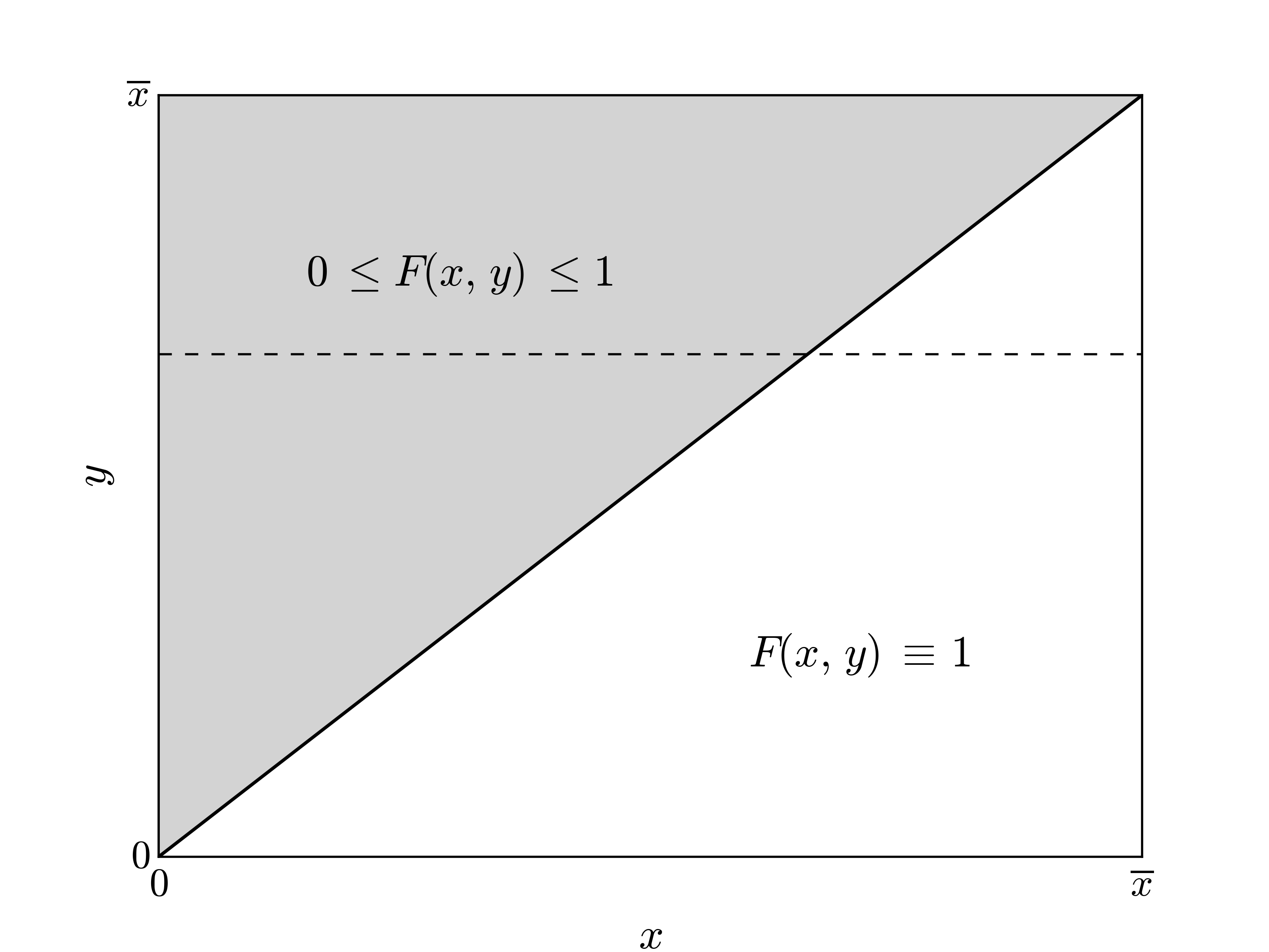
(a)

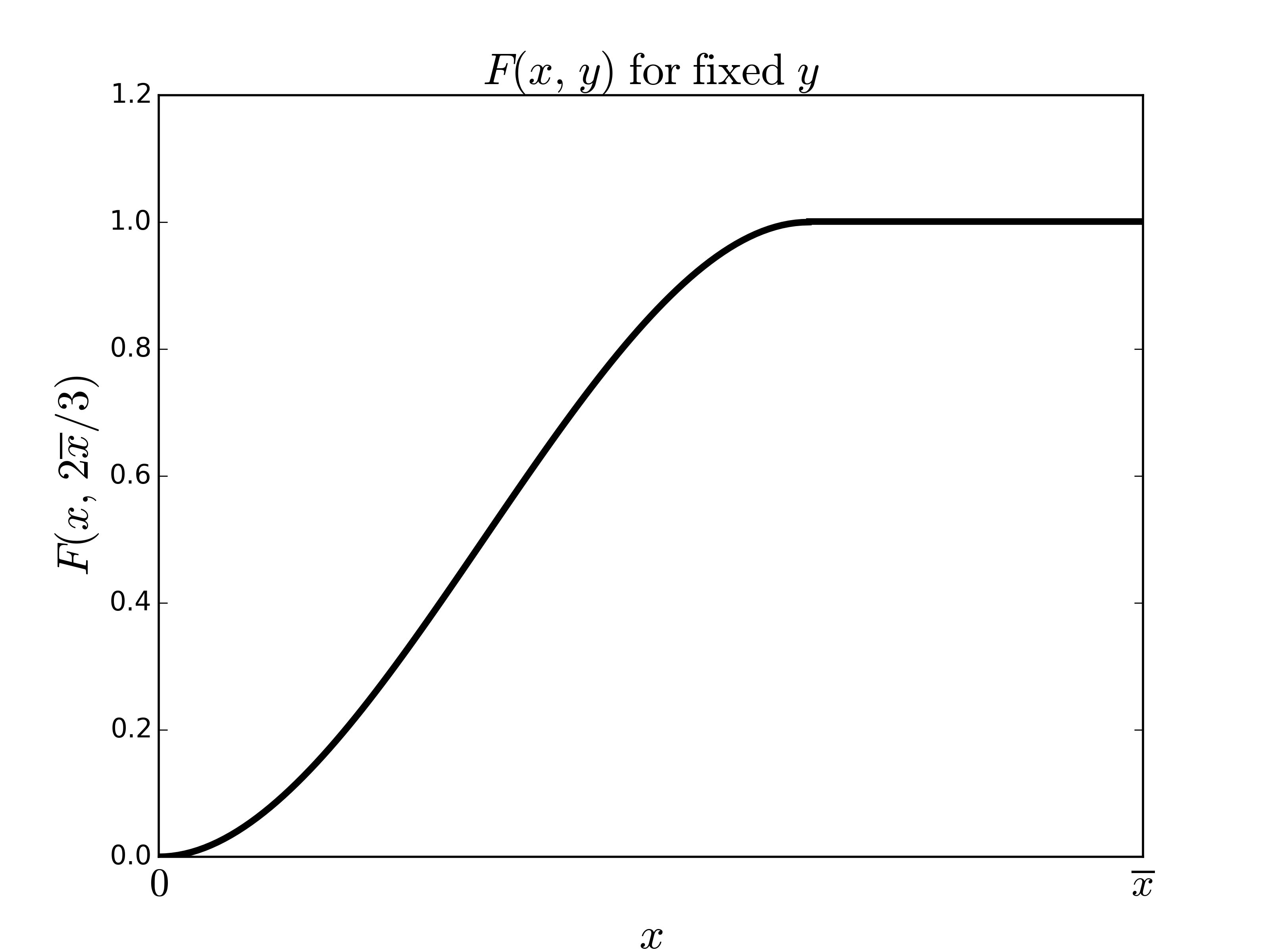
(b)

Figure 1: (a) Domain for the probability measure $F(x,\,y)$ showing admissible values for $F(x,\,y)\subset\mathscr{P}(Q)$. Dotted line is for $y=2\overline{x}/3$. (b) Example $F(x,\,2\overline{x}/3)\subset\mathscr{P}(Q)$ for fixed $y$. In this case, $\Gamma$ is a Beta distribution with $\alpha=\beta=2$

We define a metric on the space $\mathscr{F}$ to create a metric topology, and we accomplish this by making use of the well-known Prohorov metric (see [11] for a full description). Convergence in the Prohorov metric is equivalent to weak convergence, and we direct the interested reader to [17] for a summary of its relationship to a variety of other metrics on probability measures. For $F,\,\tilde{F}\in\mathscr{F}$ and fixed $y$, we use the Prohorov metric $\rho_{Proh}$ to denote the distance $\rho_{Proh}(F(\cdot,y),\,\tilde{F}(\cdot,y))$ between the measures. We extend this concept to define the metric $\rho$ on the space $\mathscr{F}(Q\times Q)$ by taking the supremum of $\rho_{Proh}$ over all $y\in Q$,

$$\rho(F,\,\tilde{F})=\sup_{y\in Q}\,\rho_{Proh}(F(\cdot,\,y),\,\tilde{F}(\cdot,\,y))\,.$$

The most widely available, high-fidelity data for flocculating particles are in the form of particle size histograms from, e.g., from flow-cytometers, Coulter counters, etc. Accordingly, we will define our inverse problem with the goal of comparing with histograms of floc sizes. Let $n_{j}(t_{i})$ represent the number of flocculated biomasses with volume between $x_{j}$ and $x_{j+1}$ at time $t_{i}$. We assume that the data is generated by an actual post-fragmentation function. In other words, $\mathbf{n}^{d}$ is representable as the partial zeroth moment of the solution

$$n_{ji}^{d}=\int_{x_{j-1}}^{x_{j}}b(t_{i},\,x;F_{0})\,dx+\mathcal{E}_{ji}$$

for some true probability-measure $F_{0}\in\mathscr{F}$. The random variables $\mathcal{E}_{ji}$ represent measurement noise. We also assume, as it is commonly assumed in statistics, that the random variables $\mathcal{E}_{ji}$ are independent, identically distributed, $E[\mathcal{E}_{ji}]=0$ and $Var[\mathcal{E}_{ji}]=\sigma^{2}<\infty$ (which is generally true for flow-cytometers [14]). Thus our inverse problem entails finding a minimizer of the least squares cost functional, defined as

$$\min_{F\in\mathscr{F}}\;J(F;\,\mathbf{n}^{d})=\min_{F\in\mathscr{F}}\;\sum_{i=1}^{N_{t}}\sum_{j=1}^{N_{x}}\left(\int_{x_{j-1}}^{x_{j}}b(t_{i},x;F)\,dx\,-\,n_{ji}^{d}\right)^{2}\,,$$ (3)

where the data $\mathbf{n}^{d}\in\mathbb{R}^{N_{x}\times N_{t}}$ consists of the number of flocs in each of the $N_{x}$ bins for floc volume at $N_{t}$ time points. The superscript $d$ denotes the dimension of the data, $d=N_{x}\times N_{t}$. The function $b$ is the solution to (1)-(2) corresponding to the probability measure $F$.

For a given data $\mathbf{n}^{d}$, the cost function $J$ may not have a unique minimizer, thus we denote a corresponding solution set of probability distributions as $\mathscr{F}^{*}(\mathbf{n}^{d}).$ We then define the distance between two such sets of solutions, $\mathscr{F}^{*}(\mathbf{n}_{1}^{d_{1}})$ and $\mathscr{F}^{*}(\mathbf{n}_{2}^{d_{2}})$ (for data $\mathbf{n}_{1}^{d_{1}}$ and $\mathbf{n}_{2}^{d_{2}}$) to be the well-known Hausdorff distance [20]

$$d_{H}(\mathscr{F}^{*}(\mathbf{n}_{1}^{d_{1}}),\,\mathscr{F}^{*}(\mathbf{n}_{2}^{d_{2}}))=\inf\{\rho(F,\tilde{\,F}):\;F\in\mathscr{F}^{*}(\mathbf{n}_{1}^{d_{1}}),\;\tilde{F}\in\mathscr{F}^{*}(\mathbf{n}_{2}^{d_{2}})\}\,.$$

2.2 Inverse Problem

In this section we will establish well-posedness of the inverse problem defined in (3). In particular, we will first show that for a given data $\mathbf{n}^{d}$ with dimension $d$ the least squares estimator defined in (3) has at least one minimizer. Next, we will investigate the behavior of minimizers of (3) as more data is collected. Specifically, we will show that the least squares estimator is consistent, i.e., as the dimension of data increases ($N_{t}\to\infty$ and $N_{x}\to\infty$) the minimizers of the estimator (3) converge to true probability measure $F_{0}$ generating the data $\mathbf{n}^{d}$.

2.2.1 Existence of the estimator.

In this section we prove that the cost functional defined in (3) possesses at least one minimizer. We use the well-known result that a continuous function on a compact metric space has a minimum. In particular, first we show that $(\mathscr{F},\,\rho)$ is a compact metric space. Next, we establish continuous dependence of the solution $b$ on the conditional probability measure $F$.

For much of the following analysis, we require the operator $g$ to satisfy a Lipschitz-type condition. We detail that condition in the following.

Condition 2.1.

Suppose that $b$ and $\tilde{b}$ are solutions to the evolution equation (1)-(2). For fixed $t$, the function $g:\,H\times\mathscr{F}\to H$ must satisfy

$$\left\|g(b,\,F)-g(\tilde{b},\,\tilde{F})\right\|\leq C\left\|b-\tilde{b}\right\|+\mathscr{T}(F,\tilde{\,F}),$$

where $C>0$, and $\mathscr{T}(F,\,\tilde{F})$ is some function such that $|\mathscr{T}(F,\,\tilde{F})|<\infty$ and $\mathscr{T}(F,\,\tilde{F})\to 0$ as $\rho(F,\,\tilde{F})\to 0$.

We begin by proving that $(\mathscr{F},\,\rho)$ is a compact metric space.

Lemma 2.2.

$(\mathscr{F},\,\rho)$ is a compact metric space.

Proof.

Consider a Cauchy sequence $\{F_{n}\}\in\mathscr{F}$. Then $\forall\;\epsilon>0,\;\exists\,N$ such that $\forall\,n,m\geq N$,

$$\sup_{y\in Q}\;\rho_{Proh}\left(F_{n}(\cdot,\,y),\,F_{m}(\cdot,\,y)\right)\,<\,\epsilon.$$

It is easy to see we have a Cauchy sequence $\{F_{n}(\cdot,\,y)\}\in\mathscr{P}_{y}(Q)$ which converges uniformly in $y\in Q$. From results in Billingsley [11], $\mathscr{P}_{y}(Q)$ is a compact metric space, there exists $F(\cdot,\,y)\in\mathscr{P}_{y}(Q)$ such that $\rho_{Proh}(F_{n}(\cdot,\,y),\,F(\cdot,\,y))<\epsilon$ for all $n\geq N$. Thus

$$\sup_{y\in Q}\;\rho_{Proh}\left(F_{n}(\cdot,\,y),\,F(\cdot,\,y)\right)\,<\,\epsilon$$

and $(\mathscr{F},\,\rho)$ is a complete metric space. In addition, since $Q\times Q$ is compact and $0\leq F(x,\,y)\leq 1$ for all $(x,\,y)\in Q\times Q,\,F\in\mathscr{F}$, $\mathscr{F}(Q\times Q)$ is totally bounded and therefore $(\mathscr{F},\,\rho)$ is a compact metric space. ∎

Now that we have a compact metric space, it remains to show that the cost functional on that space is continuous with respect to the function $F$. It suffices to prove point-wise continuity.

Lemma 2.3.

If $t\in T$, $F\in\mathscr{F}$, and the operator $g$ in (1) satisfies Condition 2.1, then the unique solution $b$ to (1) is point-wise continuous at $F\in\mathscr{F}.$ Moreover, since $\mathscr{F}$ is compact space the unique solution $b$ is uniformly continuous on $\mathscr{F}$.

Proof.

For the function $b$ to be point-wise continuous at $F$, we need to show that $\left\|b(t,\cdot;F_{i})-b(t,\cdot;F)\right\|\to 0$ as $\rho(F_{i},F)\to 0$ for $\{F_{i}\}\in\mathscr{F}$ and fixed $t$. We begin by re-writing (1) as an integral equation

$$b(t,x)=b_{0}(x)+\int_{0}^{t}g(b(s,x),F)ds\,.$$

For fixed $t$, consider $b$ to be a function of $F$

$$b(t,x;F)=b_{0}(x)+\int_{0}^{t}g(b(s,x;F),F)ds\,.$$

By definition of solutions, we have

$$\left\|b(t,\cdot;F_{i})-b(t,\cdot;F)\right\|\leq\int_{0}^{t}\left\|g(b(s,\cdot;F_{i}),F_{i})-g(b(s,\cdot;F),F)\right\|ds\,.$$

Based on Condition 2.1, we obtain

$$\left\|b(t,\cdot;F_{i})-b(t,\cdot;F)\right\|\leq C\int_{0}^{t}\left\|b(s,\cdot;F_{i})-b(s,\cdot;F)\right\|ds+\mathcal{T}(F_{i},F)\,,$$

where we define $\mathcal{T}(F_{i},F)=\int_{0}^{t_{f}}\mathscr{T}(F_{i},F)ds$, independent of $t$. An application of Gronwall’s inequality yields

$$\left\|b(t,\cdot;F_{i})-b(t,\cdot;F)\right\|\leq\mathcal{T}(F_{i},F)\,e^{\int_{0}^{t}C\,ds}\leq\mathcal{T}(F_{i},F)\,e^{C\,t_{f}}\to 0$$

since we know that $\mathcal{T}(F_{i},F)\to 0$ as $F_{i}\to F$ in $(\mathscr{F},\,\rho)$. Thus the solutions $b$ are point-wise continuous at $F\in\mathscr{F}$. ∎

We use the results of the above two lemmas to establish existence of a solution to our inverse problem.

Theorem 2.4.

There exists a solution to the inverse problem as described in (3).

Proof.

It is well known that a continuous function on a compact set obtains both a maximum and a minimum. We have shown $(\mathscr{F},\rho)$ is compact, and from Lemma 2.3, for fixed $t\in T,$ we have that $F\mapsto b(t,\cdot;F)$ is continuous. Since $J$ is continuous with respect to $F$ and we can conclude there exist minimizers for $J$. ∎

2.2.2 Consistency of the estimator.

In previous section we have proved that for a given data there exists estimators for the least squares problem. In this section we will investigate the behavior of the least squares estimators as the number of observations increase. In particular, the estimator is said to be consistent if the estimators for the data $\mathbf{n}^{d}$ converge to true probability measure $F_{0}$ as $N_{t}\to\infty$ and $N_{x}\to\infty$. Consistency of the estimators of the least squares problems are well-studied in the statistics and the results of this section follow closely the theoretical results of [10] and [8]. Hence, as in [10, Theorem 4.3] and [8, Corallary 3.2], we will make the following two assumptions required for the convergence of the estimators to the unique true probability measure $F_{0}$.

• Let us denote the space of positive functions $T\times Q\mapsto\mathbb{R}^{+}$, which are bounded and Riemann integrable by $\mathscr{R}\left(T\times Q,\,\mathbb{R}^{+}\right)$. Then, the model function $b(t,x;\,\cdot)\,:\,\mathscr{F}\to\mathscr{R}\left(T\times Q,\,\mathbb{R}^{+}\right)$ is continuous on $\mathscr{F}$.

• The functional

  $$J_{0}(F)=\sigma^{2}+\int_{T}\int_{Q}\left(b(t,x;F)-b(t,x;F_{0})\right)^{2}\,dx\,dt$$

  is uniquely (up to $L^{1}$ norm) minimized at $F_{0}\in\mathscr{F}$.

Having the required assumptions in hand, we now present the following theorem.

Theorem 2.5.

Under assumptions (A1) and (A2)

$$d_{H}\left(\mathscr{F}^{*}(\mathbf{n}^{d}),\,F_{0}\right)\to 0$$

as $N_{t}\to\infty$ and $N_{x}\to\infty$.

Proof.

The specific details of this proof are nearly identical to a similar theorem in [10] and so here we simply provide an overview. Briefly, one first shows that $J(F;\,\mathbf{n}^{d})$ converges to $J_{0}(F)$ for each $F\in\mathscr{F}$ as $N_{t}\to\infty$ and $N_{x}\to\infty$. Then, using the fact that $J_{0}(F)$ is uniquely minimized at $F_{0}$, one can show that for each sequence $\left\{F^{d}\in\mathscr{F}^{*}(\mathbf{n}^{d})\right\}$ the Prohorov distance $\rho\left(F^{d},\,F_{0}\right)$ converges to zero as $N_{t}\to\infty$ and $N_{x}\to\infty$, which yields the result. ∎

3 Approximate Inverse Problem

Since the original problem involves minimizing over the infinite dimensional space $\mathscr{F}$, pursuing this optimization is challenging without some type of finite dimensional approximation. Thus we define some approximation spaces over which the optimization problem becomes computationally tractable. Similar to the partitioning presented in [7], let $Q_{M}=\{q_{j}^{M}\}_{j=0}^{M}$ be partitions of $Q=[0,\overline{x}]$ for $M=1,2,\dots$ and

$$Q_{D}=\bigcup_{M=1}^{\infty}Q_{M}$$ (4)

where the sequences are chosen such that $Q_{D}$ is dense in $Q$.

For positive integers $M,\,L$, let the approximation space be defined as

$$\mathscr{F}^{ML} = \left\{F\in\mathscr{F}\;|\;F(x,y)=\sum_{m=1}^{M}p_{\ell m}\Delta_{q_{m}^{M}}(x)\,\mathbbm{1}_{(q_{\ell-1}^{L},\,q_{\ell}^{L}]}(y),\right.$$

$$\left.\qquad q_{m}^{M}\in Q_{M},\,q_{\ell}^{L}\in Q_{L},\,\sum_{m=1}^{\ell}p_{\ell m}=1,\,\ell=1,2,\dots,L\right\}$$

where $\Delta_{q}(x)$ is the Heaviside step function with atom $x=q$ and the function $\mathbbm{1}_{A}$ is the indicator function on the interval $A$. Next, define the space $\mathscr{F}_{D}$ as

$$\mathscr{F}_{D}=\bigcup_{M,L=1}^{\infty}\mathscr{F}^{ML}.$$

Consequently, since $Q$ is a complete, separable metric space, and by Theorem 3.1 in [6] and properties of the sup norm, $\mathscr{F}_{D}$ is dense in $\mathscr{F}$ in the $\rho$ metric. Therefore we can directly conclude that any function $F\in\mathscr{F}$ can be approximated by a sequence $\{F_{M_{j}L_{k}}\}$, $F_{M_{j}L_{k}}\in\mathscr{F}^{M_{j}L_{k}}$ such that as $M_{j},\,L_{k}\to\infty$, $\rho(F_{M_{j}L_{k}},\,F)\to 0$.

Similar to the discussion concerning Theorem 4.1 in [6], we now state the theorem regarding the continuous dependence of the inverse problem upon the given data, as well as stability under approximation of the inverse problem solution space $\mathscr{F}$.

Theorem 3.1.

Let $Q=[0,\overline{x}]$, assume that for fixed $t\in T,\;x\in Q$, $F\mapsto b(t,x,F)$ is continuous on $\mathscr{F}$, and let $Q_{D}$ be a countable dense subset of $Q$ as defined in (4). Suppose that $\mathscr{F}^{*ML}(\mathbf{n}^{d})$ is the set of minimizers for $J(F;\mathbf{n}^{d})$ over $F\in\mathscr{F}^{ML}$ corresponding to the data $\mathbf{n}^{d}$. Then, $d_{H}(\mathscr{F}^{*ML}(\mathbf{n}^{d}),\,F_{0})\to 0$ as $M,\,L,\,N_{t},\,N_{x}\to\infty$.

Proof.

Suppose that $\mathscr{F}^{*}(\mathbf{n}^{d})$ is the set of minimizers for $J(F;\mathbf{n}^{d})$ over $F\in\mathscr{F}$ corresponding to the data $\mathbf{n}^{d}$. Using continuous dependence of solutions on $F$, compactness of $(\mathscr{F},\,\rho)$, and the density of $\mathscr{F}_{D}$ in $\mathscr{F}$, the arguments follow precisely those for Theorem 4.1 in [6]. In particular, one would argue in the present context that any sequence $F_{d}^{*ML}\in\mathscr{F}^{*ML}(\mathbf{n}^{d})$ has a subsequence $F_{d_{k}}^{*M_{j}L_{i}}$ that converges to a $\tilde{F}\in\mathscr{F}^{*}(\mathbf{n}^{d})$. Therefore, we can claim that

$$d_{H}\left(\mathscr{F}^{*ML}(\mathbf{n}^{d}),\,\mathscr{F}^{*}(\mathbf{n}^{d})\right)\to 0$$ (5)

as $M,\,L,\,N_{t},\,N_{x}\to\infty$. Conversely, simple triangle inequality yields that

$$d_{H}(\mathscr{F}^{*ML}(\mathbf{n}^{d}),\,F_{0})\leq d_{H}\left(\mathscr{F}^{*ML}(\mathbf{n}^{d}),\,\mathscr{F}^{*}(\mathbf{n}^{d})\right)+d_{H}\left(\mathscr{F}^{*}(\mathbf{n}^{d}),\,F_{0}\right)\,.$$

This is in turn, from (5) and Theorem 2.5, implies that $d_{H}(\mathscr{F}^{*ML}(\mathbf{n}^{d}),\,F_{0})$ converges to zero as $M,\,L,\,N_{t},\,N_{x}\to\infty$. ∎

Since we do not have direct access to an analytical solution to (1), our efforts are focused on the solving the approximate inverse problem

$$\min_{F\in\mathcal{F}}J^{N}(F,\mathbf{n}^{d})=\min_{f\in\mathcal{F}}\sum_{i=1}^{N_{t}}\sum_{j=1}^{N_{x}}\left(\int_{x_{j-1}}^{x_{j}}b^{N}(t_{i},x_{j};F)dx-n_{ji}^{d}\right)^{2}\,.$$ (6)

Here, $N_{t}$ is the number of data observations, $N_{x}$ is the number of data bins for floc volume, and $b^{N}$ is the semi-discrete approximation to $b$. In Section 4, we will define a uniformly (in time) convergent discretization scheme and its corresponding approximation space $H^{N}\subset H$. The discretized version of (6) is represented by

$$\qquad b_{t}^{N} = g^{N}(b^{N},F)$$ (7)

$$b^{N}(0,x) = b_{0}^{N}(x)$$ (8)

where $g^{N}:H^{N}\times\mathscr{F}\to H^{N}$ denotes the discretized version of $g$. We will need that $g^{N}$ exhibits a type of local Lipschitz continuity and accordingly define the following condition.

Condition 3.2.

Suppose that the discretization given in (7)-(8) is a convergent scheme. Let $(b^{N},F),\,(\tilde{b}^{N},\tilde{F})\in H^{N}\times\mathscr{F}$. For fixed $t$, the function $g^{N}:\,H^{N}\times\mathscr{F}\to H^{N}$ must satisfy

$$\left\|g^{N}(b^{N},F)-g^{N}(\tilde{b}^{N},\tilde{F})\right\|\leq C_{N}\left\|b^{N}-\tilde{b}^{N}\right\|+\mathscr{T}^{N}(F,\tilde{F}),$$

where $C_{N}>0$, and $\mathscr{T}^{N}(F,\tilde{F})$ is some function such that $|\mathscr{T}^{N}(F,\tilde{F})|<\infty$ and $\mathscr{T}^{N}(F,\tilde{F})\to 0$ as $\rho(F,\tilde{F})\to 0$.

General method stability [9] requires $b^{N}(t,x;F_{i})\to b(t,x;F)$ as $F_{i}\to F$ in the $\rho$ metric and as $N\to\infty$; we will now prove this.

Lemma 3.3.

Let $t\in T$, $F\in\mathscr{F},$and $\{F_{i}\}\in\mathscr{F}$ such that $\lim_{i\to\infty}\rho(F_{i},F)=0$. For fixed $N$, if $b^{N}(t,x;F_{i})$ is the solution to (16)-(17) and Condition 3.2 holds, then $b^{N}$ is pointwise continuous at $F\in\mathscr{F}$.

Proof.

The proof of this lemma is identical to that for Lemma 2.3. We first recast (7) as an integral equation and then apply Condition 3.2 and Gronwall’s inequality to obtain the desired result.∎

Corollary 3.4.

Under Condition 3.2 and Lemma 3.3, we can conclude that $\left\|b^{N}(t,\cdot;F_{N})-b(t,\cdot;F)\right\|\to 0$ as $N\to\infty$ uniformly in $t$ on $I$.

Proof.

A standard application of the triangle inequality yields

$$\left\|b^{N}(t,\cdot;F_{N})-b(t,\cdot;F)\right\| \leq \left\|b^{N}(t,\cdot;F_{N})-b^{N}(t,\cdot;F)\right\|$$

$$\quad+\left\|b^{N}(t,\cdot;F)-b(t,\cdot;F)\right\|\,.$$

The first term converges by Lemma 3.3, while the second term converges because the proposed numerical scheme is assumed to converge uniformly. ∎

With this corollary, we now consider the existence of a solution to the approximate inverse problem in (6), as well as the solution’s dependence on the given data $\mathbf{n}^{d}$.

Theorem 3.5.

There exists solutions to both the original and approximate inverse problems in (3) and (6), respectively. Moreover, for fixed data $\mathbf{n}^{d}$, there exist a subsequence of the estimators $\left\{F_{N}\right\}_{N=1}^{\infty}$ of (6) that converge to a solution of the original inverse problem (3).

Proof.

As noted above, $(\mathscr{F},\rho)$ is compact. By Lemmas 2.3 and 3.3, we have that both $F\mapsto b(t,x;F)$ and $F\mapsto b^{N}(t,x;F)$, for fixed $t\in T$, are continuous with respect to $F$. We therefore know there exist minimizers in $\mathscr{F}$ to the original and approximate cost functionals $J$ and $J^{N}$ respectively.

Let $\{F_{N}^{*}\}\in\mathscr{F}$ be any sequence of solutions to (6) and $\{F_{N_{k}}^{*}\}$ a convergent (in $\rho$) subsequence of minimizers. Recall that minimizers are not necessarily unique, but one can always select a convergent subsequence of minimizers in $\mathscr{F}$. Denote the limit of this subsequence with $F^{*}$. By the minimizing properties of $F_{N_{k}}^{*}\in\mathscr{F}$, we then know that

$$J^{N_{k}}(F_{N_{k}}^{*},\mathbf{n}^{d})\leq J^{N_{k}}(F,\mathbf{n}^{d})\qquad\text{for all }F\in\mathscr{F}.$$ (9)

By Corollary 3.4, we have the convergence of $b^{N}(t,x;F_{N})\to b(t,x;F)$ and thus $J^{N}(F_{N})\to J(F)$ as $N\to\infty$ when $\rho(F_{N},F)\to 0$. Thus in the limit as $N_{k}\to\infty$, the inequality in (9) becomes

$$J(F^{*},\mathbf{n}^{d})\leq J(F,\mathbf{n}^{d})\qquad\text{for all }F\in\mathscr{F}$$

with $F^{*}$ providing a (not necessarily unique) minimizer of (3).∎

Theorem 3.6.

Assume that for fixed $t\in T$, $F\mapsto b(t,x;F)$ is continuous on $\mathscr{F}$ in $\rho$, $b^{N}$ is the approximate solution to the forward problem given (16)-(17), $J^{N}$ is the approximation given in (6), and $Q_{D}$ a countable dense subset of $Q$ as defined in (4). Moreover, suppose that $\mathscr{F}_{N}^{*ML}(\mathbf{n}^{d})$ is the set of minimizers for $J^{N}(F;\mathbf{n}^{d})$ over $F\in\mathscr{F}^{ML}$ corresponding to the data $\mathbf{n}^{d}$. Similarly, suppose that $\mathscr{F}^{*}(\mathbf{n}^{d})$ is the set of minimizers for $J(F;\mathbf{n}^{d})$ over $F\in\mathscr{F}$ corresponding to the data $\mathbf{n}^{d}$. Then, $d_{H}(\mathscr{F}_{N}^{*ML}(\mathbf{n}^{d}),\,F_{0})\to 0$ as $N,\,M,\,L,\,N_{t},\,N_{x}\to\infty$.

Proof.

Observe that a simple triangle inequality yields

$$d_{H}\left(\mathscr{F}_{N}^{*ML}(\mathbf{n}^{d}),\,F_{0}\right)\leq d_{H}\left(\mathscr{F}_{N}^{*ML}(\mathbf{n}^{d}),\,\mathscr{F}^{*ML}(\mathbf{n}^{d})\right)+d_{H}\left(\mathscr{F}^{*ML}(\mathbf{n}^{d}),\,F_{0}\right)\,.$$

Therefore, combining the arguments of Theorem 3.1 and Theorem 3.5, we readily obtain that $d_{H}\left(\mathscr{F}_{N}^{*ML}(\mathbf{n}^{d}),\,F_{0}\right)$ converges to zero as $N,\,M,\,L,\,N_{t},\,N_{x}\to\infty$. ∎

With the results of these two theorems, we can claim that both there exists a solution to the inverse problem and it is continuously dependent on the given data. We have established method stability under approximation of the state space and parameter space of our inverse problem. Therefore we can conclude general well-posedness of the inverse problem.

4 Example Illustration

The particular model we study here is the size-structured flocculation dynamics of the microorganisms in suspension and is given by the following integro-differential equation

$$\qquad b_{t} = \mathcal{A}[b]+\mathcal{B}[b]+\mathcal{R}[b],$$ (10)

$$b(t,\,0) = 0,$$ (11)

$$b(0,\,x) = b_{0}(x),$$ (12)

where $b(t,\,x)\,dx$ is the number of aggregates with volumes in $[x,\,x+dx]$ at time $t$, and $\mathcal{A}$, $\mathcal{B}$ and $\mathcal{R}$ are the aggregation, breakage (fragmentation) and removal operators, respectively. We consider $x\in Q=[0,\,\overline{x}]$, where $\overline{x}$ is the maximum floc volume and $t\in T=[0,\,t_{f}]$, $t_{f}<\infty$. The aggregation, fragmentation and removal functions are defined by:

$$\mathcal{A}[p](t,\,x) := \frac{1}{2}\int_{0}^{x}k_{a}(x-y,\,y)p(t,\,x-y)p(t,\,y)\,dy$$ (13)

$$-p(t,\,x)\int_{0}^{\overline{x}}k_{a}(x,\,y)p(t,\,y)\,dy\,,$$

$$\mathcal{B}[p](t,\,x) := \int_{x}^{\overline{x}}\Gamma(x;\,y)k_{f}(y)p(t,\,y)\,dy-\frac{1}{2}k_{f}(x)p(t,\,x)$$ (14)

and

$$\mathcal{R}[p](t,\,x):=-\mu(x)p(t,\,x)\,.$$ (15)

where $k_{a}(x,\,y)$ is the aggregation kernel, describing the rate at which flocs of volume $x$ and $y$ combine to form a floc of volume $x+y$. The aggregation kernel is symmetric function and $k_{a}(x,\,y)=0$ for $x+y>\overline{x}$. The fragmentation kernel $k_{f}(x)$ describes the rate at which a floc of volume $x$ fragments. The function $\Gamma(x,\,y)$ is the post-fragmentation probability density, for the conditional probability of producing a daughter floc of size $x$ from a mother floc of size $y$. This probability density is used to characterize the stochastic nature of floc fragmentation (e.g., see the discussions in [12, 18, 4, 13]).

In [13], we proposed a model for bacterial floc breakage based upon hydrodynamic arguments and predicted a post fragmentation density $\Gamma$. The eventual goal (and the topic for a future paper) is to unify the theoretical results (in this work and in [12, 13]) with experimental evidence to validate (or refute) our proposed fragmentation model. We now consider the application of this framework to the system in (10)-(12). For fixed $t\in I,\,$$b(t,\cdot)\in H$, $F\in\mathscr{F}$, consider the right side of (10), represented by (1),

$$g(b,\,F)=\mathcal{A}[b]+\mathcal{B}[b;\,F]+\mathcal{R}[b]\,.$$

To show that $g$ satisfies the locally Lipschitz property of Condition 2.1, we need the following two lemmas.

Lemma 4.1.

Suppose that $k_{f},\,\mu\in L^{\infty}(Q)$ and $k_{a},\,\Gamma\in L^{\infty}\left(Q\times Q\right)$. The evolution equation (10)-(12) is well-posed on $H=L^{1}\left(Q,\,\mathbb{R}^{+}\right)$ and for any compact set $T=[0,\,t_{f}]$ and $b_{0}\geq 0$, the classical solution of (10)-(12) satisfies

$$C_{0}=\sup_{t\in T,\,x\in Q}\left|b(t,\,x)\right|<\infty\,.$$

Furthermore, the operator $\mathcal{A}+\mathcal{R}$ is locally Lipschitz

$$\left\|\mathcal{A}[b]+\mathcal{R}[b]-\mathcal{A}[\tilde{b}]-\mathcal{R}[\tilde{b}]\right\|\leq C_{1}\left\|b-\tilde{b}\right\|$$

where $C_{1}=3C_{0}\left\|k_{a}\right\|_{\infty}+\left\|\mu\right\|_{\infty}$.

Proof.

For the proof of the first part we refer readers to [12, §3]. To show that $\mathcal{A}+\mathcal{R}$ is locally Lipschitz, first observe that

$$\left\|\mathcal{A}[b]-\mathcal{A}[\tilde{b}]\right\| \leq \frac{1}{2}\int_{Q}\left|\int_{0}^{x}k_{a}(x-y,\,y)b(x-y)b(y)\,dy\right.$$

$$\left.-\int_{0}^{x}k_{a}(x-y,\,y)\tilde{b}(x-y)\tilde{b}(y)\,dy\right|dx$$

$$+\int_{Q}\left|b(x)\int_{Q}k_{a}(x,\,y)b(y)\,dy-\tilde{b}(x)\int_{Q}k_{a}(x,\,y)\tilde{b}(y)\,dy\right|\,dx$$

$$\leq \left\|k_{a}\right\|_{\infty}\left[\frac{1}{2}\int_{Q}\left|\int_{0}^{x}b(x-y)\left(b(y)-\tilde{b}(y)\right)\,dy\right|\,dx\right.$$

$$+\frac{1}{2}\int_{Q}\left|\int_{0}^{x}\tilde{b}(y)\left(b(x-y)-\tilde{b}(x-y)\right)\,dy\right|\,dx$$

$$+\int_{Q}\left|b(x)\int_{Q}\left(b(y)-\tilde{b}(y)\right)\,dy\right|\,dx$$

$$\left.+\int_{Q}\left|\tilde{b}(x)\int_{Q}\left(b(y)-\tilde{b}(y)\right)\,dy\right|\,dx\right]\,.$$

At this point applying Young’s inequality [3, Theorem 2.24] for the first two integrals yields the desired result

$$\left\|\mathcal{A}[b]-\mathcal{A}[\tilde{b}]\right\| \leq \left\|k_{a}\right\|_{\infty}\left[\frac{1}{2}\left\|b\right\|\left\|b-\tilde{b}\right\|+\frac{1}{2}\left\|\tilde{b}\right\|\left\|b-\tilde{b}\right\|\right.$$

$$\left.+\left\|b\right\|\left\|b-\tilde{b}\right\|+\left\|\tilde{b}\right\|\left\|b-\tilde{b}\right\|\right]$$

$$\leq 3C_{0}\left\|k_{a}\right\|_{\infty}\left\|b-\tilde{b}\right\|\,.$$

∎

The above lemma establishes that the classical solution of (10)-(12) is bounded on $T\times Q$. Moreover, since the space of Riemann integrable functions are dense on $L^{1}(Q,\,\mathbb{R}^{+})$, we tacitly assume that the classical solution is also Riemann integrable. Therefore, the evolution equation (10)-(12) satisfies consistency conditions of Theorem 2.5, and thus the inverse problem defined in (3) is well-posed for this particular application.

Lemma 4.2.

The fragmentation operator $\mathcal{B}$ satisfies the locally Lipschitz property of Condition 2.1.

Proof.

Examining the fragmentation term, we find

$$\left\|\mathcal{B}(b,F)-\mathcal{B}(\tilde{b},\tilde{F})\right\| \leq \left\|\frac{1}{2}k_{f}(x)\left(\tilde{b}(t,\,x)-b(t,\,x)\right)\right\|$$

$$+\left\|\int_{x}^{\overline{x}}k_{f}(y)\left(b(t,\,y)\,\Gamma(x,y)-\tilde{b}(t,\,y)\,\tilde{\Gamma}(x,y)\right)dy\right\|$$

$$\leq \frac{1}{2}C_{\text{frag}}\left\|b-\tilde{b}\right\|+K\left\|\int_{Q}b(t,\,y)\left(\Gamma(x,y)-\tilde{\Gamma}(x,y)\right)dy\right\|$$

$$+C_{\text{frag}}\left\|\int_{Q}\left(b(t,\,y)-\tilde{b}(t,\,y)\right)\tilde{\Gamma}(x,y)\,dy\right\|$$

where $C_{\text{frag}}=\left\|k_{f}\right\|_{\infty}$. The second term on the right hand side becomes

$$C_{\text{frag}}\left\|\int_{Q}b(t,\,y)\left(\Gamma(x,y)-\tilde{\Gamma}(x,y)\right)dy\right\| \leq C_{\text{frag}}\int_{Q}\int_{Q}\left|b(t,\,y)\right|\left|\Gamma(x,y)-\tilde{\Gamma}(x,y)\right|dy\,dx$$

$$\leq C_{\text{frag}}\int_{Q}\left|b(t,\,y)\right|\int_{Q}\left|\Gamma(x,y)dx-\tilde{\Gamma}(x,y)dx\right|dy$$

$$\leq C_{\text{frag}}\int_{Q}\left|b(t,\,y)\right|\left(\int_{Q}\left|dF_{y}-d\tilde{F}_{y}\right|\right)dy$$

$$\leq C_{\text{frag}}\sup_{y\in Q}\int_{Q}\left|dF_{y}-d\tilde{F}_{y}\right|\int_{Q}\left|b(t,\,y)\right|dy$$

$$\leq C_{\text{frag}}\overline{x}C_{0}\sup_{y\in Q}\int_{Q}\left|dF_{y}-d\tilde{F}_{y}\right|$$

Since $\int_{Q}\left|dF_{y}-d\tilde{F}_{y}\right|\to 0$ is equivalent to $\rho_{Proh}(F_{y},\tilde{F}_{y})\to 0$ , we know that

$$\sup_{y\in Q}\int_{Q}\left|dF_{y}-d\tilde{F}_{y}\right|\to 0\quad\text{as}\quad\rho(F,\tilde{F})\to 0.$$

Therefore,

$$C_{\text{frag}}\left\|\int_{Q}b(y)\left(\Gamma(x,y)-\tilde{\Gamma}(x,y)\right)dy\right\|\to 0\quad\text{as}\quad\rho(F,\,\tilde{F})\to 0.$$

Similar analysis for the third term leads to the bound

$$C_{\text{frag}}\left\|\int_{Q}\left(b(y)-\tilde{b}(t,y)\right)\tilde{\Gamma}(x,y)\,dy\right\|\leq C_{\text{frag}}\overline{x}\left\|\Gamma\right\|_{\infty}\left\|b-\tilde{b}\right\|.$$

Combining these results we find the overall fragmentation term can be bounded by

$$\left\|\mathcal{B}(b,\phi)-\mathcal{B}(\tilde{b},\tilde{\phi})\right\|\leq C_{\text{frag}}\left(\frac{1}{2}+\overline{x}\left\|\Gamma\right\|_{\infty}\right)\left\|b-\tilde{b}\right\|+\mathscr{T}(F,\,\tilde{F}).$$

∎

Claim 4.3.

The function $g$ satisfies the locally Lipschitz property of Condition 2.1.

Proof.

Consider

$$\left\|g(b,F)-g(\tilde{b},\tilde{F})\right\| = \left\|\mathcal{A}[b]-\mathcal{A}[\tilde{b}]+\mathcal{B}[b;F]-\mathcal{B}[\tilde{b};\tilde{F}]+\mathcal{R}[b]-\mathcal{R}[\tilde{b}]\right\|$$

$$\leq \left\|\mathcal{A}[b]-\mathcal{A}[\tilde{b}]\right\|+\left\|\mathcal{B}[b;F]-\mathcal{B}[\tilde{b};\tilde{F}]\right\|+\left\|\mathcal{R}[b]-\mathcal{R}[\tilde{b}]\right\|\,.$$

Using the Lipschitz constants from the fragmentation and aggregation terms,

$$\left\|g(b,\phi)-g(\tilde{b},\tilde{\phi})\right\|\leq C\left\|b-\tilde{b}\right\|+\mathscr{T}(F,\,\tilde{F})$$

where $C=C_{\text{frag}}\left(\frac{1}{2}+\overline{x}\left\|\Gamma\right\|_{\infty}\right)+C_{1}$. ∎

Therefore, since the function $g$ satisfies Condition 2.1, we can conclude well-posedness of the inverse problem for identifying the post-fragmentation probability density, $\Gamma(x,y)$, found in the model for flocculation dynamics of bacterial aggregates described in (10)-(12).

4.1 Numerical Implementation

We first form an approximation to $H$. We define basis elements

$$\beta_{i}^{N}(x)=\left\{\begin{array}[]{cc}1;&x_{i-1}^{N}\leq x\leq x_{i}^{N}\,;\,i=1,\ldots,N\\ 0;&\mbox{otherwise}\end{array}\right.$$

for positive integer $N$ and $\{x_{i}^{N}\}_{i=0}^{N}$ a uniform partition of $[0,\overline{x}]=[x_{0}^{N},x_{N}^{N}]$, and $\Delta x=x_{j}^{N}-x_{j-1}^{N}$ for all $j$. The $\beta^{N}$ functions form an orthogonal basis for the approximate solution space

$$H^{N}=\left\{h\in H\;|\;h=\sum_{i=1}^{N}\alpha_{i}\beta_{i}^{N},\;\alpha_{i}\in\mathbb{R}\right\},$$

and accordingly, we define the orthogonal projections $\pi^{N}:\,H\mapsto H^{N}$

$$\pi^{N}h=\sum_{j=1}^{N}\,\alpha_{j}\beta_{j}^{N},\qquad\text{where}\>\alpha_{j}=\frac{1}{\Delta x}\,\int_{x_{j-1}^{N}}^{x_{j}^{N}}\,h(x)\,dx.$$

Thus our approximating formulations of (10), (12) becomes the following system of $N$ ODEs for $b^{N}\in H^{N}$ and $F\in\mathscr{F}$:

$$b_{t}^{N} = \pi^{N}\left(\mathcal{A}[b^{N}]+\mathcal{B}[b^{N};F]+\mathcal{R}[b^{N}]\right),$$ (16)

$$b^{N}(0,x) = \pi^{N}b_{0}(x)\,,$$ (17)

where

$$\pi^{N}\mathcal{A}[b^{N}] = \left(\begin{array}[]{c}-\alpha_{1}\sum_{j=1}^{N-1}k_{a}(x_{1},\,x_{j})\alpha_{j}\Delta x\\ \frac{1}{2}k_{a}(x_{1},x_{1})\alpha_{1}\alpha_{1}\Delta x-\alpha_{2}\sum_{j=1}^{N-2}k_{a}(x_{2},\,x_{j})\alpha_{j}\Delta x\\ \vdots\\ \frac{1}{2}\sum_{j=1}^{N-2}k_{a}(x_{j},x_{N-1-j})\alpha_{j}\alpha_{N-1-j}\Delta x-\alpha_{N-1}k_{a}(x_{N-1},\,x_{1})\alpha_{1}\Delta x\\ \frac{1}{2}\sum_{j=1}^{N-1}k_{a}(x_{j},x_{N-j})\alpha_{j}\alpha_{N-j}\Delta x\end{array}\right)$$

and

$$\pi^{N}\left(\mathcal{B}[b^{N};F]+\mathcal{R}[b^{N}]\right) = \left(\begin{array}[]{c}\sum_{j=2}^{N}\Gamma(x_{1};x_{j})k_{f}(x_{j})\alpha_{j}\Delta x-\frac{1}{2}k_{f}(x_{1})\alpha_{1}-\mu(x_{1})\alpha_{1}\\ \sum_{j=3}^{N}\Gamma(x_{2};x_{j})k_{f}(x_{j})\alpha_{j}\Delta x-\frac{1}{2}k_{f}(x_{2})\alpha_{2}-\mu(x_{2})\alpha_{2}\\ \vdots\\ \Gamma(x_{N-1};x_{N})k_{f}(x_{N})\alpha_{N}\Delta x-\frac{1}{2}k_{f}(x_{N-1})\alpha_{N-1}-\mu(x_{N-1})\alpha_{N-1}\\ -\frac{1}{2}k_{f}(x_{N})\alpha_{N}-\mu(x_{N})\alpha_{N}\end{array}\right)\,.$$

In the following lemma we show that the numerical scheme satisfies Condition 3.2.

Claim 4.4.

The function $g^{N}:H^{N}\times\mathscr{F}\to H^{N}$ as defined by

$$g^{N}(b^{N},F)=\mathcal{A}[b^{N}]+\mathcal{B}[b^{N};F]+\mathcal{R}[b^{N}]$$

satisfies the Lipschitz-type property in Condition 3.2.

Proof.

We consider the integrand

$$\left\|\pi^{N}\left(\mathcal{A}[b^{N}(t,x;\tilde{F})]+\mathcal{B}[b^{N}(t,x;\tilde{F})]-\mathcal{A}[b^{N}(t,x;F)]-\mathcal{B}[b^{N}(t,x;F)]\right)\right\|\,,$$

and note that

$$\begin{array}[]{cc}\leq&\left\|\pi^{N}\right\|\left(\left\|\mathcal{A}[b(t,x;\tilde{F})]-\mathcal{A}[b^{N}(t,x;F)]\right\|\right.\\ &\qquad\left.+\left\|\mathcal{B}[b^{N}(t,x;\tilde{F})]-\mathcal{B}[b^{N}(t,x;F)]\right\|\right)\,.\end{array}$$

The induced ($L^{1}$-) norm on the projection operator will not be an issue as

$$\left\|\pi^{N}\right\| = \sup_{h\in H,\left\|h\right\|=1}\left\|\pi^{N}h\right\|$$

$$= \sup_{h\in H,\left\|h\right\|=1}\left\|\sum_{j=1}^{N}\frac{\beta_{j}^{N}(\cdot)}{\Delta x}\int_{x_{j-1}^{N}}^{x_{j}^{N}}h(x)dx\right\|$$

$$= 1\,.$$

As illustrated in the proof of Claim 4.3 above, the bounding constants for $\mathcal{A}$ and $\mathcal{B}$ are $C_{\text{agg}}$ and $\frac{3}{2}C_{\text{frag}}$, respectively.

Combining these results,

$$\left\|b^{N}(t,x;\tilde{F})-b^{N}(t,x;F)\right\|\leq C_{N}\left\|b^{N}(t,x;\tilde{F})-b^{N}(t,x;F)\right\|+\mathcal{T}^{N}(\tilde{F},F)$$

where $\mathcal{T}^{N}(\tilde{F},F)=\int_{0}^{t_{f}}\pi^{N}\mathscr{T}(\tilde{F},F)ds$, independent of $t$, and $C_{N}=\left\|k_{f}\right\|_{\infty}\left(\frac{1}{2}+\overline{x}\left\|\Gamma\right\|_{\infty}\right)+3C_{0}\left\|k_{a}\right\|_{\infty}+\left\|\mu\right\|_{\infty}\,.$ ∎

Corollary 4.5.

The semi-discrete solutions to (16) converge uniformly in norm to the unique solution of (10) on a bounded time interval as $N\to\infty$.

Proof.

From results in [12], we can obtain semi-discrete solutions $b^{N}$ to the forward problem that converge uniformly in norm to the unique solution of (10)-(12) on a bounded time interval as $N\to\infty$.

For fixed $N$, we rewrite (16) in integral form and consider

$$\left\|b^{N}(t,x;F)-\pi^{N}b(t,x;F)\right\| \leq \int_{0}^{t}\left\|\pi^{N}\left(\mathcal{R}[b^{N}(s,x;F)]-\mathcal{R}[b(s,x;F)]\right)\right\|ds$$

$$+\int_{0}^{t}\left\|\pi^{N}\left(\mathcal{A}[b^{N}(s,x;F)]+\mathcal{B}[b(s,x;F)]\right.\right.$$

$$\left.\left.-\mathcal{A}[b^{N}(s,x;F)]-\mathcal{B}[b(s,x;F]\right)\right\|ds.$$

for $t\in T$. Our strategy is to use the fact that our discretized version of $g$ is locally Lipschitz and then apply Gronwall’s inequality. We refer readers to [1, 12] for the detailed discussion about the convergence of the numerical scheme. ∎

4.2 Results

As an initial investigation into the utility of this approach, we applied the method to the problem of flocculation dynamics. In [13], we have shown that the post-fragmentation density function greatly depends on the parent floc size. In particular, we found that the resulting post-fragmentation density for large parent flocs resembles a Beta distribution with $\alpha=\beta=0.5$. For small flocs, however, the resulting density resembles a Beta distribution with $\alpha=\beta=2$. Towards this end, we applied the framework presented in this paper to these two different post-fragmentation functions. In Figure 2, data were generated from the forward problem by assuming a post-fragmentation density function,

$$\Gamma_{\text{true}}(x,y)=\mathbbm{1}_{[0,\,y]}(x)\frac{6x(y-x)}{y^{3}}\,.$$

Similarly, in Figure 3, data were generated with a post-fragmentation density function,

$$\Gamma_{\text{true}}(x,y)=\mathbbm{1}_{[0,\,y]}(x)\frac{1}{\pi\sqrt{x(y-x)}}\,.$$

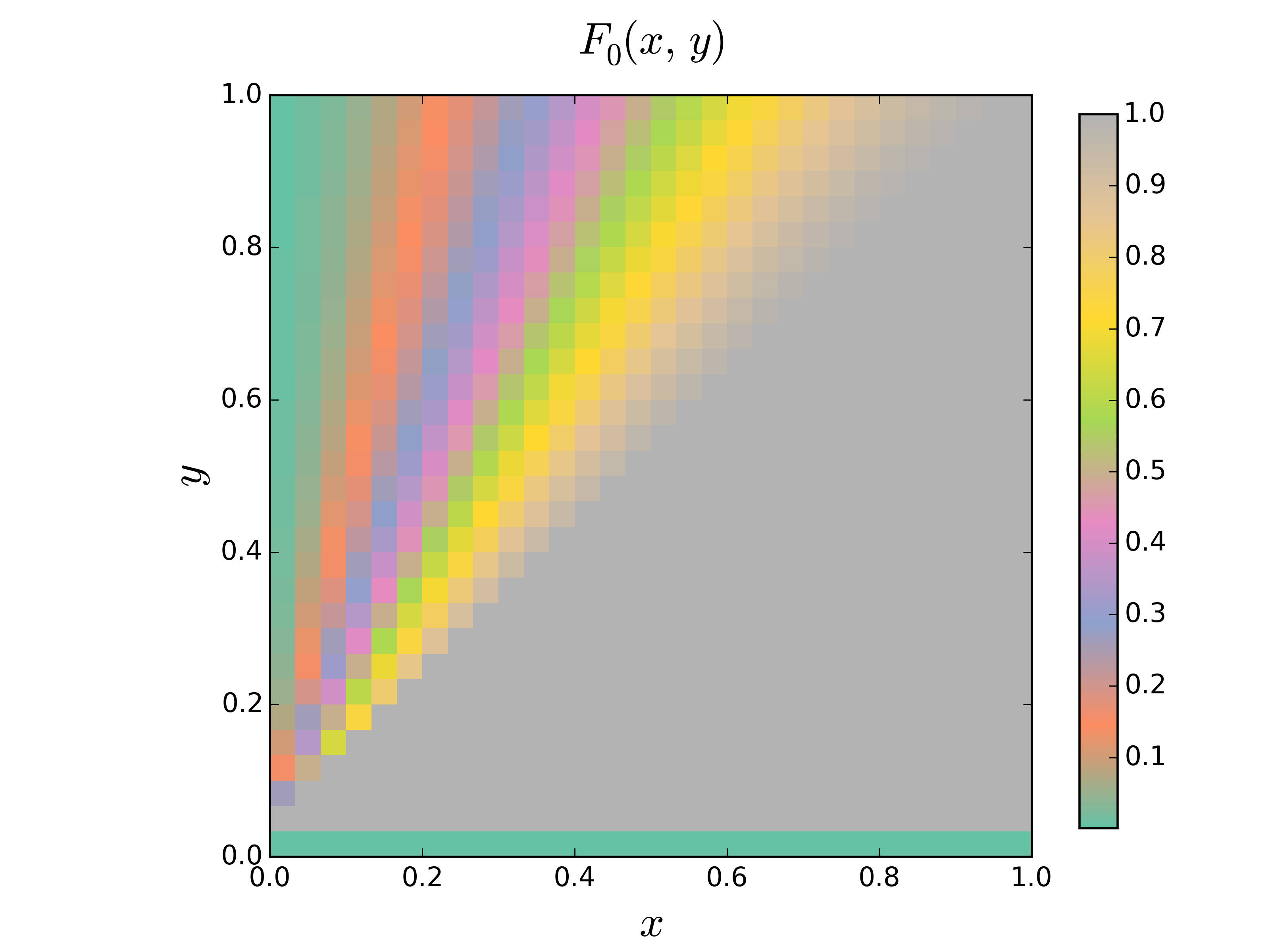
(a)

(b)

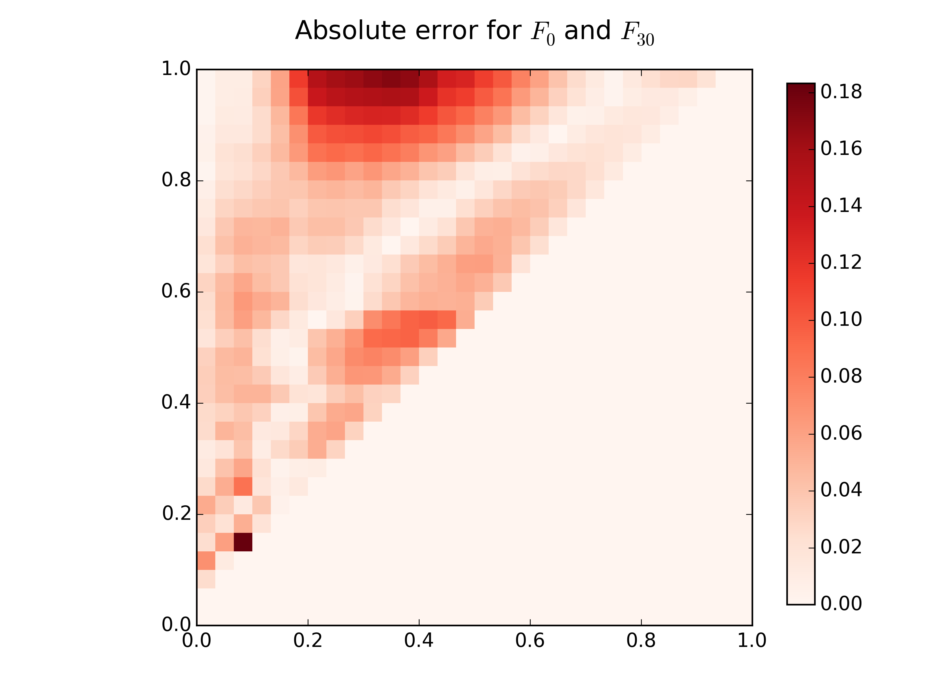
(c)

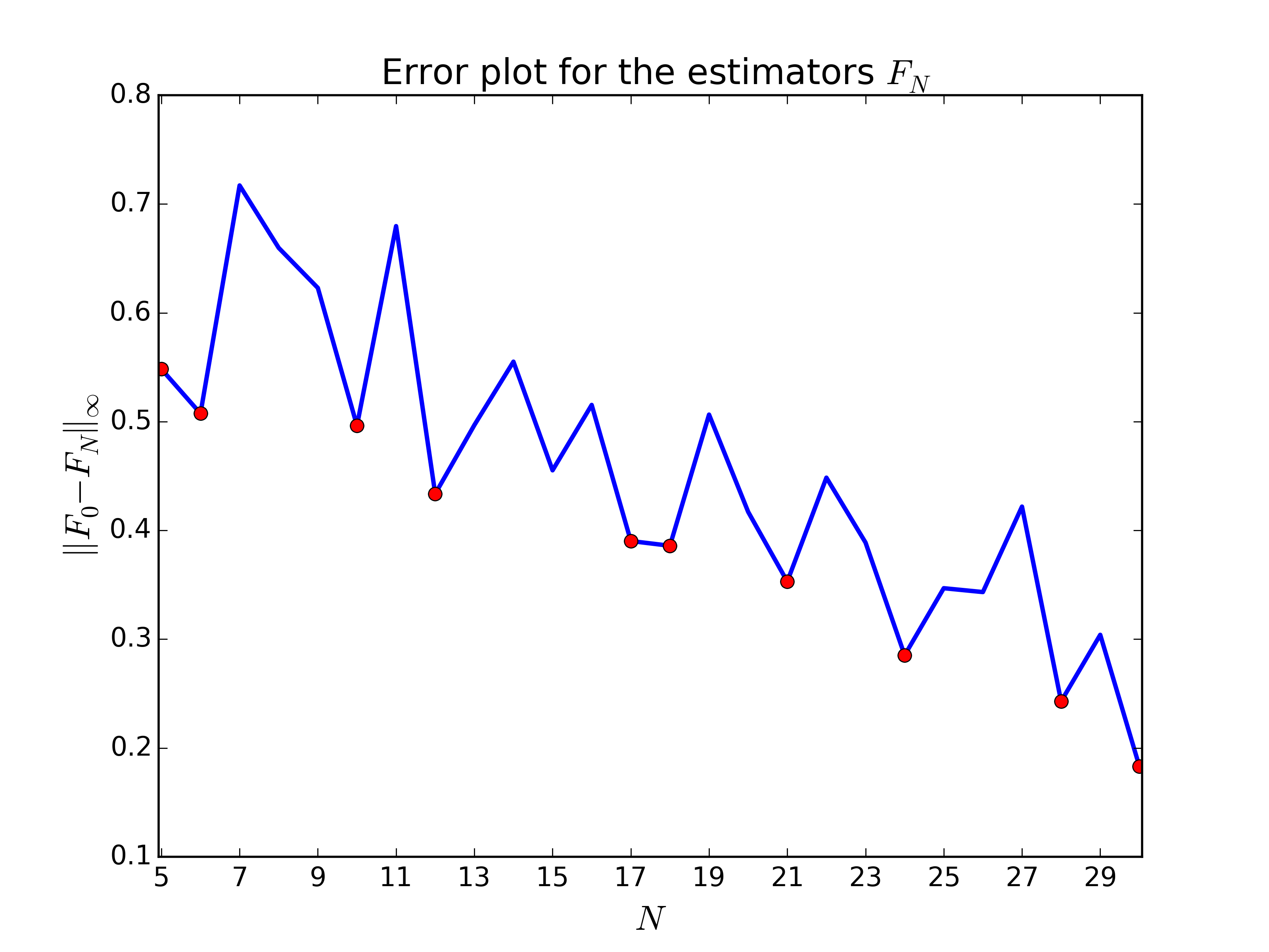
(d)

Figure 2: Simulation results for pseudo-data generated with Beta distribution with $\alpha=\beta=2$ (a) Post-fragmentation density used to generate test data (true post-fragmentation density). (b) Results of the optimization scheme based on these data and an initial density function uniform in $x$. (c) Absolute error for true probability measure $F_{0}$ and the approximate estimator $F_{30}$. (d) Error plots for the sequence of estimators $\left\{F_{N}\right\}_{N=5}^{30}$ . Solid red dots indicate the convergent subsequence of the estimators.

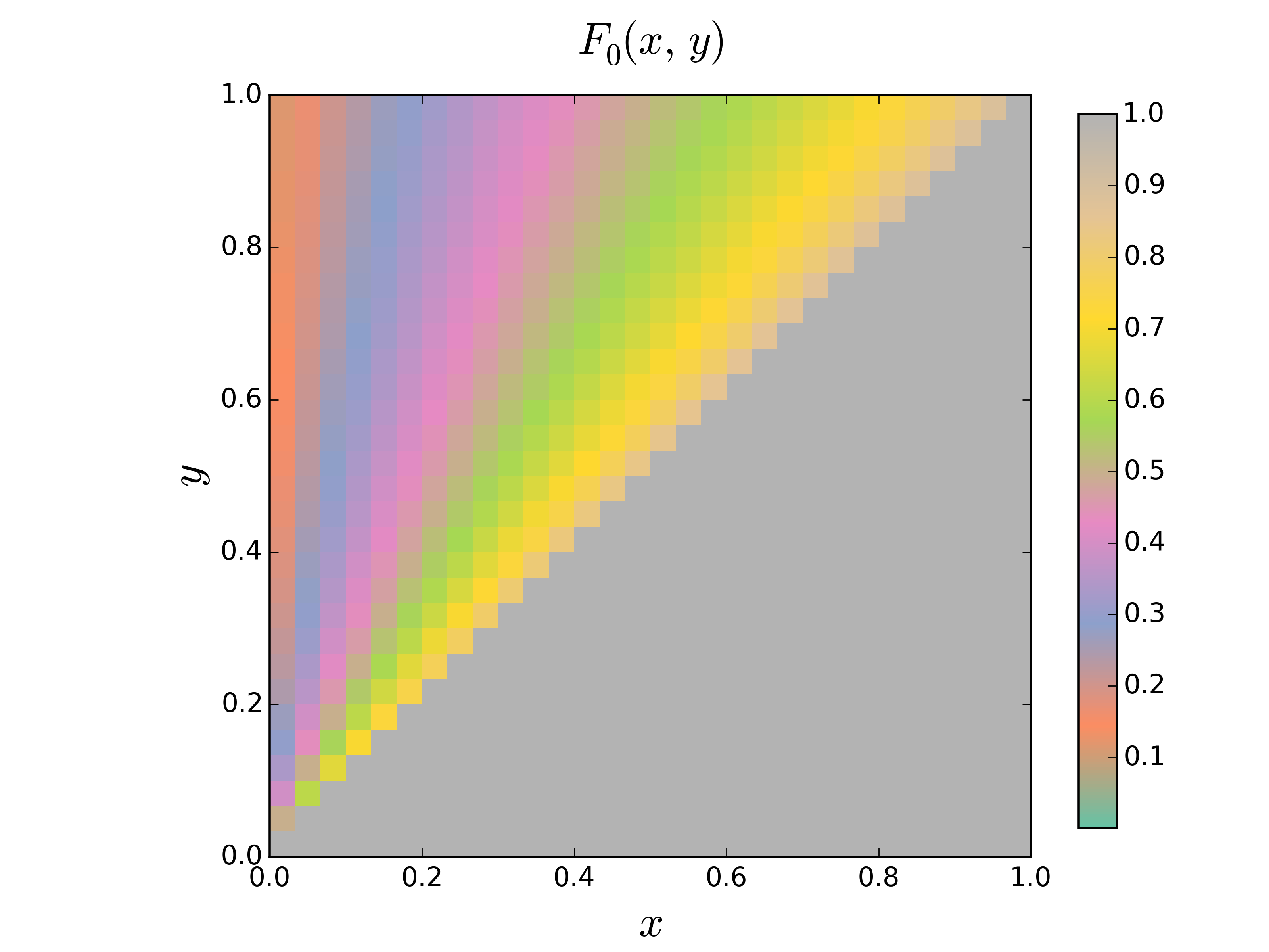
(a)

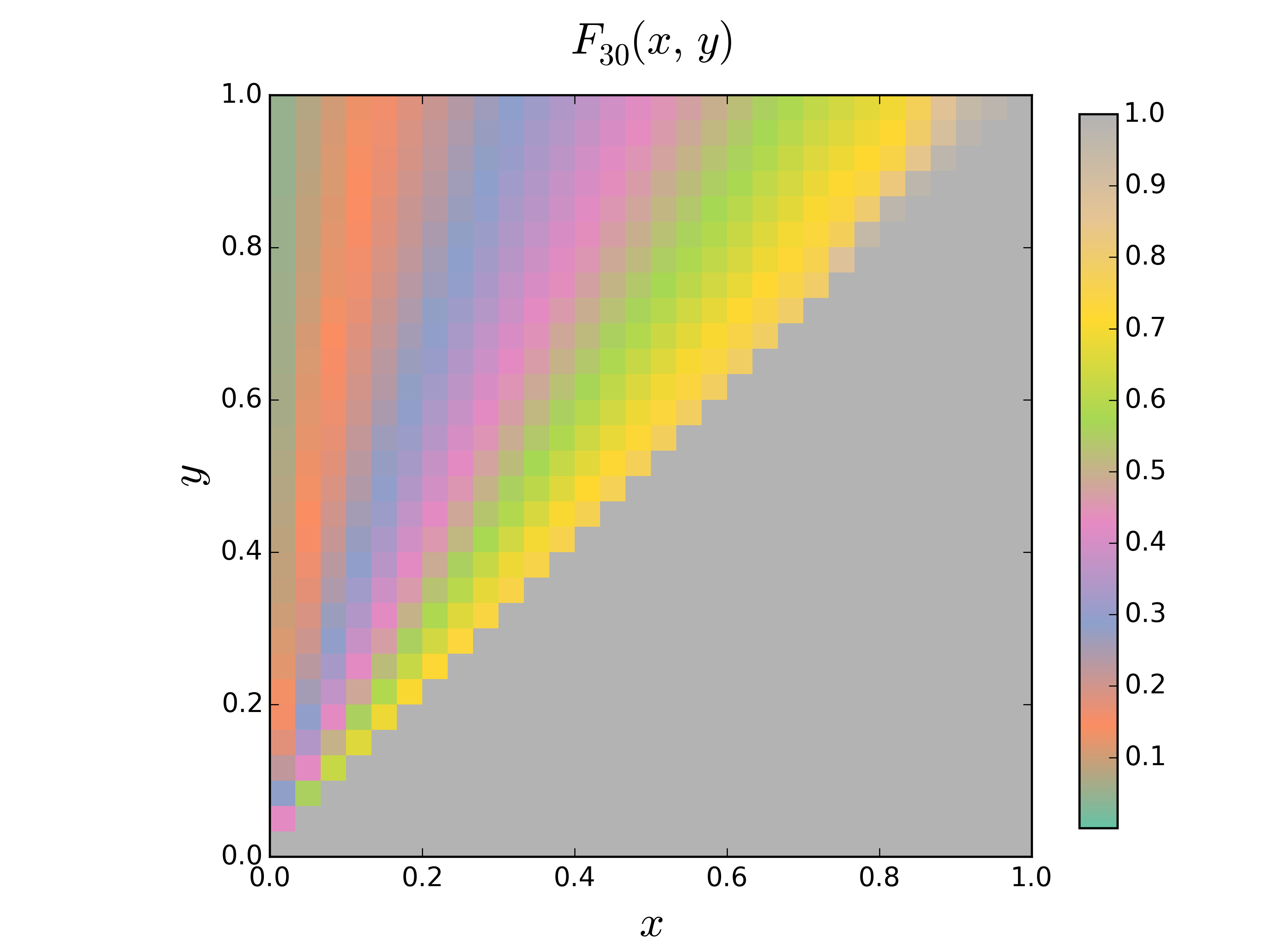
(b)

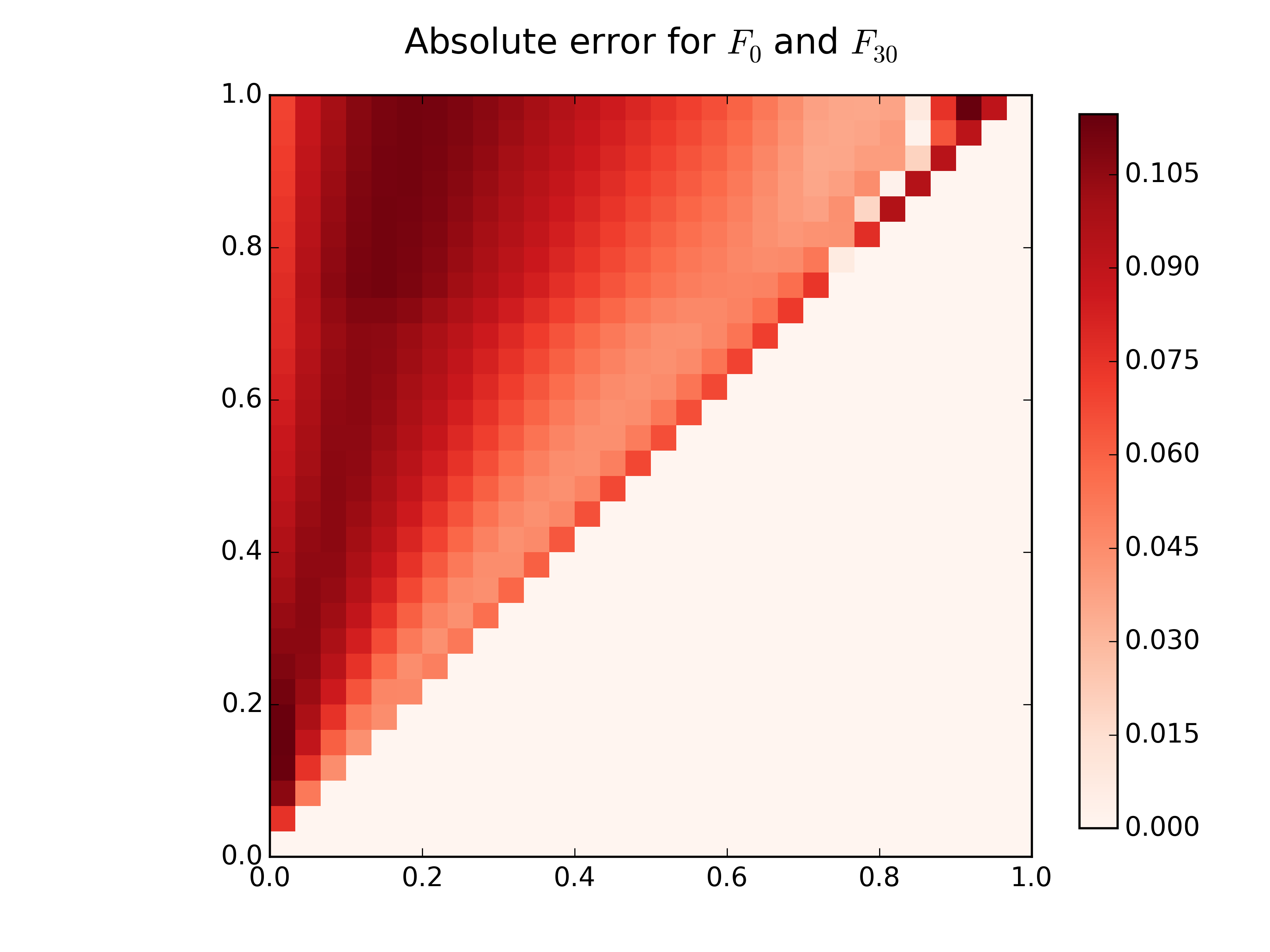
(c)

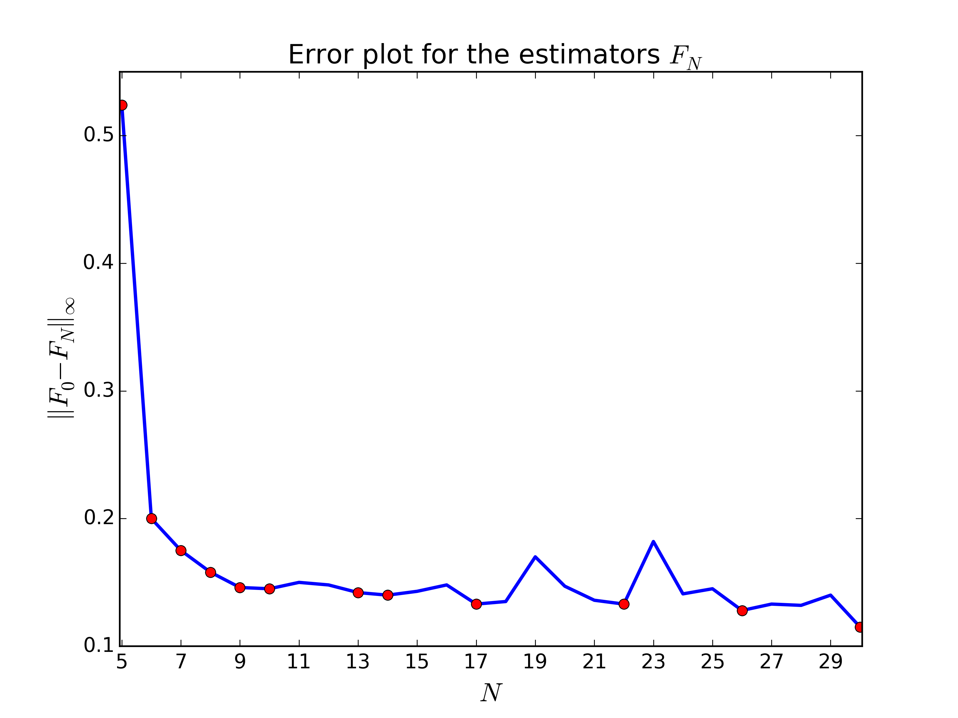
(d)

Figure 3: Simulation results for pseudo-data generated with Beta distribution with $\alpha=\beta=0.5$ (a) Post-fragmentation density used to generate test data. (b) Results of the optimization scheme based on these data and an initial density function uniform in $x$. (c) Absolute error for true probability measure $F_{0}$ and the approximate estimator $F_{30}$. (d) Error plots for the sequence of estimators $\left\{F_{N}\right\}_{N=5}^{30}$ . Solid red dots indicate the convergent subsequence of the estimators.

To describe the aggregation within a laminar shear field (orthokinetic aggregation) we used the kernel,

$$k_{a}(x,\,y)=10^{-6}\left(x^{1/3}+y^{1/3}\right)^{3}\,,$$

proposed by von Smoluchowski [24]. As in [12, 2, 21, 22] we assume that the breakage and removal rate of a floc of volume $x$ is proportional to its size,

$$k_{f}(x)=10^{-1}x^{1/3}\quad\mu(x)=10^{-1}x^{1/3}\,.$$

We also note that constants for the rate functions were chosen to emphasize the fragmentation as a driving factor. The simulations were run with initial size-distribution $b_{0}(x)=10^{3}\exp(-x)$ on $Q=[0,\,1]$ for $t\in[0,\,1]$. These data serve as the “observed” data $\mathbf{n}^{d}$. Nonlinear constrained optimization employing the sequential least squares algorithm as implemented in Python fmin_slsqp was used to minimize the cost functional in (6). The optimization was seeded with an initial density comprised of a uniform density in $x$ for fixed $y$. Naturally, we constrained $\Gamma(\cdot,y)$ to be a probability density for each fixed $y$, i.e.,

$$\int_{0}^{y}\Gamma(x;\,y)\,dx=1\text{ for all }y\in(0,\,\overline{x}].$$

Our discretization uses $M=L=N_{x}=N$. We found that having more comparison points in time was critical to observe the expected error convergence in N. To illustrate this effect, we let $N_{t}=N+40$. The result of the optimization for $N=30$, $F_{30}(x,y)$, is shown in Figure 2. Absolute error for the true probability measure $F_{0}$ and the approximate estimator $F_{30}$ is depicted in Figure  2c. Convergence in Prohorov metric implies the uniform convergence of probability measures [17], i.e.,

$$\sup_{(x,\,y)\in Q\times Q}\left|F(x,\,y)-\tilde{F}(x,\,y)\right|\leq\rho(F,\,\tilde{F})\,.$$

Towards this end, in Figure 2d, we have illustrated error plots for the sequence of estimators $\left\{F_{N}\right\}_{N=5}^{30}$ . As it has been predicted in Theorem 3.5 the sequence of the estimators has a subsequence (indicated by solid red dots) which is convergent to true probability measure $F_{0}$. Our results for larger $N$ confirm that trend continues for $N>30$.

5 Concluding Remarks

Our efforts here are motivated by a class of mathematical models which characterize a random process, such as fragmentation, by a probability distribution. We are concerned with the inverse problem for inferring the probability distribution, and present the specific problem for the flocculation dynamics of aggregates in suspension which motivated this study. We then developed the mathematical framework in which we establish well-posedness of the inverse problem for inferring the probability distribution. We also include results for overall method stability for numerical approximation, confirming a computationally feasible methodology. Finally, we verify that our motivating example in flocculation dynamics conforms to the developed framework, and illustrate its utility by identifying a sample distribution.

We originally proposed the flocculation model in [12] and this work is one piece of a larger effort aimed at pushing the boundaries for identifying microscale phenomena from size-structured population measurements. In particular, we are interested in fragmentation. The model proposed in [13] uses knowledge of the hydrodynamics to predict a breakage event and thus the post fragmentation density $\Gamma$. With this work, we now have a tool to bridge the gap between the experimental and modeling efforts for fragmentation. And, a future paper will focus on using experimental evidence to validate (or refute) our proposed fragmentation model.

References

References

- [1] A. S. Ackleh, Parameter estimation in a structured algal coagulation-fragmentation model, Nonlinear Analysis, 28 (1997), pp. 837–854.
- [2] A. S. Ackleh and B. G. Fitzpatrick, Modeling aggregation and growth processes in an algal population model: analysis and computations, Journal of Mathematical Biology, 35 (1997), pp. 480–502.
- [3] R. Adams and J. Fournier, Sobolev spaces, Elsevier Ltd, Oxford, UK, 2003.
- [4] M. U. Bäbler, M. Morbidelli, and J. Baldyga, Modelling the breakup of solid aggregates in turbulent flows, Journal of Fluid Mechanics, 612 (2008), pp. 261–289.
- [5] J. Banasiak and W. Lamb, Coagulation, fragmentation and growth processes in a size structured population, Discrete and Continuous Dynamical Systems - Series B, 11 (2009), pp. 563–585.
- [6] H. T. Banks and K. L. Bihari, Modeling and Estimating Uncertainty in Parameter Estimation, Inverse Problems, 17 (2001), pp. 95–111.
- [7] H. T. Banks and D. M. Bortz, Inverse problems for a class of measure dependent dynamical systems, Journal of Inverse and Ill-posed Problems, 13 (2005), pp. 103–121.
- [8] H. T. Banks and B. G. Fitzpatrick, Statistical methods for model comparison in parameter estimation problems for distributed systems, Journal of Mathematical Biology, 28 (1990), pp. 501–527.
- [9] H. T. Banks and K. Kunisch, Estimation Techniques for Distributed Parameter Systems, vol. 1 of Systems & Control: Foundations & Applications, Birkhäuser, Boston, MA, 1989.
- [10] H. T. Banks and W. C. Thompson, Least Squares Estimation of Probability Measures in the Prohorov Metric Framework, N.C. State Center for Research in Scientific Computation Technical Report, (2012).
- [11] P. Billingsley, Convergence of Probability Measures, John Wiley & Sons, New York, NY, 1968.
- [12] D. M. Bortz, T. L. Jackson, K. A. Taylor, A. P. Thompson, and J. G. Younger, Klebsiella pneumoniae Flocculation Dynamics, Bull. Math. Biology, 70 (2008), pp. 745–68.
- [13] E. Byrne, S. Dzul, M. Solomon, J. Younger, and D. M. Bortz, Postfragmentation density function for bacterial aggregates in laminar flow, Physical Review E, 83 (2011), p. 041911.
- [14] Z. Darzynkiewicz, J. P. Robinson, and H. A. Crissman, Flow Cytometry, in Methods in Cell Biology, Academic Press, San Diego, CA, 2nd ed., 1994, pp. 1–697.
- [15] V. T. DeVita, S. Lawrence, Theodore, and S. A. Rosenberg, Cancer: Principles and Practice of Oncology, vol. 1, Lippincott Williams & Wilkins, 2008.
- [16] C. D. Gamma and C. L. Jimeno, Rock fragmentation control for blasting cost minimization and environmental impact abatement, in Rock Fragmentation by Blasting, P. P. Roy, ed., A. A. Balkema Publishers, Amsterdam, The Netherlands, 1993, p. 273.
- [17] A. L. Gibbs and F. E. Su, On Choosing and Bounding Probability Metrics, International Statistical Review, 70 (2002), pp. 419–435.
- [18] B. Han, S. Akeprathumchai, S. R. Wickramasinghe, and X. Qian, Flocculation of biological cells: Experiment vs. theory, AIChE Journal, 49 (2003), pp. 1687–1701.
- [19] N. Ilana, M. Elkinb, and I. Vlodavsky, Regulation, function and clinical significance of heparanase in cancer metastasis and angiogenesis, The International Journal of Biochemistry & Cell Biology, 38 (2006), p. 2018.
- [20] J. L. Kelley, General Topology, Van Nostrand-Reinhold, Princeton, NJ, 1955.
- [21] I. Mirzaev and D. M. Bortz, Criteria for linearized stability for a size-structured population model, arXiv:1502.02754, (2015).
- [22] , Stability of steady states for a class of flocculation equations with growth and removal, arXiv:1507.07127, (2015).
- [23] P.-A. Persson, R. Holmberg, and J. Lee, Rock Blasting and Explosives engineering, CRC Press, 1994.
- [24] M. van Smoluchowski, Versuch einer mathematischen theorie der koagulation kinetic kolloider losungen, Zeitschrift für physikalische Chemie, 92 (1917), pp. 129–168.
- [25] J. B. Wyckoff, J. G. Jones, J. S. Condeelis, and J. E. Segall, A critical step in metastasis: in vivo analysis of intravasation at the primary tumor., Cancer research, 60 (2000), pp. 2504–2511.