Regular rotating electrically charged black holes and solitons

in nonlinear electrodynamics minimally coupled to gravity

Irina Dymnikova^a,b and Evgeny Galaktionov^a

^aA.F. Ioffe Physico-Technical Institute, Politekhnicheskaja 26, St.Petersburg, 194021 Russia

^bDepartment of Mathematics and Computer Science, University of Warmia and Mazury,

Słoneczna 54, 10-710 Olsztyn, Poland; e-mail: irina@uwm.edu.pl

Abstract

In nonlinear electrodynamics coupled to gravity, regular spherically symmetric electrically charged solutions satisfy the weak energy condition and have obligatory de Sitter centre. By the Gürses-Gürsey algorithm they are transformed to spinning electrically charged solutions asymptotically Kerr-Newman for a distant observer. Rotation transforms de Sitter center into de Sitter vacuum surface which contains equatorial disk $r=0$ as a bridge. We present general analysis of the horizons, ergoregions and de Sitter surfaces, as well as the conditions of the existence of regular solutions to the field equations. We find asymptotic solutions and show that de Sitter vacuum surfaces have properties of a perfect conductor and ideal diamagnetic, violation of the weak energy condition is prevented by the basic requirement of electrodynamics of continued media, and the Kerr ring singularity is replaced with the superconducting current.

Journal Reference: Class. Quant. Grav. 32 (2015) 165015

1 Introduction

The Kerr-Newman electrically charged rotating solution to the Maxwell-Einstein equations [1]

$$ds^{2}=\frac{(2mr-e^{2})-\Sigma}{\Sigma}dt^{2}+\frac{\Sigma}{\Delta}dr^{2}+\Sigma d\theta^{2}-\frac{2a(2mr-e^{2})\sin^{2}\theta}{\Sigma}dtd\phi$$

$$+\biggl{(}r^{2}+a^{2}+\frac{(2mr-e^{2})a^{2}\sin^{2}\theta}{\Sigma}\biggr{)}\sin^{2}\theta d\phi^{2};~{}~{}\Delta=r^{2}-2mr+a^{2}+e^{2},$$ (1)

where $\Sigma$-function and the associated electromagnetic potential read

$$\Sigma=r^{2}+a^{2}\cos^{2}\theta;~{}~{}A_{i}=-\frac{er}{\Sigma}[1;0,0,-a\sin^{2}\theta],$$ (2)

was obtained from the Reissner-Nordström electrovacuum solution with using the complex coordinate transformation discovered by Newman and Janis [2].

The Kerr-Newman geometry has at most two horizons $r_{\pm}=m\pm\sqrt{m^{2}-(a^{2}+e^{2})}$, and implies the same value of the gyromagnetic ratio $g=2$, as predicted for a spinning particle by the Dirac equation [3]. In the case appropriate for particles, $a^{2}+e^{2}>m^{2}$, there are no Killing horizons, the manifold is geodesically complete (except for geodesics which reach the singularity), and any point can be connected to any other point by both a future and a past directed time-like curve. Closed time-like curves originate in the region where $g_{\phi\phi}<0$, can extend over the whole manifold and cannot be removed by taking a covering space [3].

The Kerr-Newman solution belongs to the Kerr family of solutions to the source-free Maxwell-Einstein equations, and represents the exterior fields of a rotating charged body [3]. The source models for the Kerr-Newman exterior can be roughly divided into disk-like [4, 5, 6], shell-like [7, 8, 9], bag-like [10, 11, 12, 13, 14, 15, 16], and string-like ([17] and references therein).

The problem of matching the Kerr-Newman exterior to a rotating material source does not have a unique solution, since one is free to choose arbitrarily the boundary between the exterior and the interior [4], not speaking about freedom in choosing an interior model itself.

On the other hand, one can study equations describing a dynamical system to get information about its basic properties rather than postulate properties of a source which could give rise to the Kerr-Newman fields. In the case of an electromagnetically interacting structure the appropriate equations come from nonlinear electrodynamics coupled to gravity (NED-GR).

Nonlinear electrodynamics was proposed by Born and Infeld as founded on two basic points: to consider electromagnetic field and particles within the frame of one physical entity which is electromagnetic field; to avoid letting physical quantities become infinite [21]. This program can be realized in nonlinear electrodynamics coupled to gravity. Source-free NED-GR equations admit regular causally safe axially symmetric asymptotically Kerr-Newman solutions [22], which describe regular rotating charged black holes and electromagnetic spinning solitons.

The key point is that for any gauge-invariant Lagrangian ${\cal L}(F)$, stress-energy tensor of electromagnetic field in the spherically symmetric case has the algebraic structure

$$T^{t}_{t}=T^{r}_{r}~{}~{}~{}(p_{r}=-\rho).$$ (3)

Regular spherically symmetric solutions with stress-energy tensors specified by (3) satisfying the weak energy condition (non-negativity of density as measured by any local observe), have obligatory de Sitter center with $p=-\rho$ [23, 24, 25, 26]. The mass $m$ of an object is generically related to de Sitter vacuum and breaking of space-time symmetry from the de Sitter group in the origin [25].In the NED-GR regular solutions interior de Sitter vacuum provides a proper cut-off on self-interaction divergent for a point charge [27, 22].

The regular spherical solutions generated by (3) belong to the Kerr-Schild class [28, 15, 29] and can be transformed by the Gürses-Gürsey algorithm [30] into regular axially symmetric solutions which describe regular rotating electrically charged objects, asymptotically Kerr-Newman for a distant observer [31, 22]. Rotation transforms the de Sitter center into de Sitter vacuum disk which has properties of a perfect conductor and ideal diamagnetic and displays superconducting behavior within a single spinning object [22, 32].

In this paper we address the question of the existence and asymptotic behaviour of solutions to the dynamical field equations which define the basic generic features of regular rotating electrically charged objects. In the paper [15] it was noted that rotation leads to violation of the weak energy condition (WEC) in interior regions of neutral regular rotating configurations. Violation of WEC was found for regular solutions obtained with the Newman-Janis algorithm from the Hayward and Bardeen metrics [33], for rotating regular solutions obtained by postulating a metric $g_{\mu\nu}$ and calculating $T_{\mu\nu}$ from the Einstein equations [34], and for the Ayón-Beato-Garcia solution transformed to rotational form with the Newman-Janis algorithm [35]. Here we study the weak energy condition for NED-GR electrically charged rotating regular structures with an arbitrary Lagrangian ${\cal L}(F)$, and generic behaviour of electromagnetic fields on the vacuum surfaces ($p+\rho=0$), beyond which the weak energy condition could be violated.

The paper is organized as follows. In Sect. 2 we present and analyze the basic equations. In Sect. 3 we address the question of the existence of horizons and ergoregions, and present interior de Sitter vacuum surfaces. In Sect. 4 we study electromagnetic fields and in Sect 5 behaviour of fields in regular interiors. In Sect. 6 we summarize and discuss the results.

2 Basic equations

Nonlinear electrodynamics minimally coupled to gravity is described by the action

$$S=\frac{1}{16\pi G}\int{d^{4}x\sqrt{-g}[R-{\cal L}(F)]};~{}~{}~{}F=F_{\mu\nu}F^{\mu\nu},$$ (4)

where $R$ is the scalar curvature, and $F_{\mu\nu}=\partial_{\mu}A_{\nu}-\partial_{\nu}A_{\mu}$ is the electromagnetic field. The gauge-invariant electromagnetic Lagrangian ${\cal L}(F)$ is an arbitrary function of $F$ which should have the Maxwell limit, ${\cal L}\rightarrow F,~{}{\cal L}_{F}\rightarrow 1$ in the weak field regime.

Variation with respect to $A^{\mu}$ and $g_{\mu\nu}$ yields the dynamic field equations

$$\nabla_{\mu}({\cal L}_{F}F^{\mu\nu})=0;$$ (5)

$$\nabla_{\mu}{{}^{*}}F^{\mu\nu}=0;~{}~{}^{\star}F^{\mu\nu}=\frac{1}{2}\eta^{\mu\nu\alpha\beta}F_{\alpha\beta};~{}~{}\eta^{0123}=-\frac{1}{\sqrt{-g}},$$ (6)

where greek indices run from 0 to 3 and ${\cal L}_{F}=d{\cal L}/dF$, and the Einstein equations $G_{\mu\nu}=-\kappa T_{\mu\nu}$ with the stress-energy tensor

$$\kappa T^{\mu}_{\nu}=-2{\cal L}_{F}F_{\nu\alpha}F^{\mu\alpha}+\frac{1}{2}\delta^{\mu}_{\nu}{\cal L};~{}~{}~{}\kappa=8\pi G.$$ (7)

NED-GR equations do not admit regular spherically symmetric solutions with the Maxwell center [36], but they admit regular solutions with the de Sitter center in which field tension goes to zero, while the energy density of the electromagnetic vacuum $T_{t}^{t}$ achieves its maximal finite value which represents the de Sitter cutoff on the self-energy density [27]. The question of correct description of NED-GR regular electrically charged structures by the Lagrange dynamics is clarified in [37]. Regular spherical solutions satisfying (3) are described by the metric

$$ds^{2}=g(r)dt^{2}-\frac{dr^{2}}{g(r)}-r^{2}d\Omega^{2};~{}~{}g(r)=1-\frac{2{\cal M}(r)}{r};~{}~{}{\cal M}(r)=4\pi\int_{0}^{r}{~{}\tilde{\rho}(x)x^{2}dx},$$ (8)

with the electromagnetic density $\tilde{\rho}(r)=T^{t}_{t}(r)$ from (7). This metric has the de Sitter asymptotic as $r\rightarrow 0$ and the Reissner-Nordström asymptotic as $r\rightarrow\infty$ [27].

Spherically symmetric solutions of the Einstein equations specified by (3) belong to the Kerr-Schild class [29, 15]. By the Gürses-Gürsey algorithm they can be transformed into axially symmetric regular solutions describing rotating objects [30]. The Kerr-Schild metric has the form

$$g_{\mu\nu}=\eta_{\mu\nu}+\frac{2f(r)}{\Sigma}k_{\mu}k_{\nu},$$ (9)

where $\eta_{\mu\nu}$ is the Minkowski metric and $k_{\mu}$ is a vector field tangent to the Kerr principal null congruence. Metric (9) involves a function $f(r)=r{\cal M}(r)$ which comes from a spherically symmetric solution [30]. For the Kerr-Newman geometry $f(r)=mr-e^{2}/2$. The parameter $r$ is defined as an affine parameter along either of two principal null congruences. The surfaces of constant $r$ are the oblate confocal ellipsoids of revolution given by [38]

$$r^{4}-(x^{2}+y^{2}+z^{2}-a^{2})r^{2}-a^{2}z^{2}=0$$ (10)

which degenerate, for $r=0$, to the equatorial disk

$$x^{2}+y^{2}\leq a^{2},~{}~{}z=0$$ (11)

centered on the symmetry axis and bounded by the ring

$$x^{2}+y^{2}=a^{2},~{}~{}z=0.$$ (12)

In the Kerr-Newman metric (1) the ring (12) comprises the Kerr singularity of the Kerr-Newman geometry [38].

The Cartesian coordinates $x,y,z$ are related to the Boyer-Lindquist coordinates $r,\theta,\phi$ by

$$x^{2}+y^{2}=(r^{2}+a^{2})\sin^{2}\theta;~{}~{}z=r\cos\theta.$$ (13)

In the Boyer-Lindquist coordinates the Gürses-Gürsey metric reads

$$ds^{2}=\frac{2f-\Sigma}{\Sigma}dt^{2}+\frac{\Sigma}{\Delta}dr^{2}+\Sigma d\theta^{2}-\frac{4af\sin^{2}\theta}{\Sigma}dtd\phi+\biggl{(}r^{2}+a^{2}+\frac{2fa^{2}\sin^{2}\theta}{\Sigma}\biggr{)}\sin^{2}\theta d\phi^{2},$$ (14)

where the Lorentz signature is [- + + +], and

$$\Delta(r)=r^{2}+a^{2}-2f(r);~{}~{}\Sigma=r^{2}+a^{2}\cos^{2}\theta.$$ (15)

For the Kerr-Newman geometry $2f(r)=2mr-e^{2}$ can change the sign which leads to causality violation related to regions where $g_{\phi\phi}<0$. For regular spherical solutions satisfying the weak energy condition, $f(r)=r{\cal M}(r)$ is non-negative function since ${\cal M}(r)$ is monotonically growing from $4\pi\tilde{\rho}(0)r^{3}/3$ as $r\rightarrow 0$ to $m-e^{2}/2r$ as $r\rightarrow\infty$ [27]. This guarantees the causal safety on the whole manifold due to $f(r)\geq 0$ and $g_{\phi\phi}>0$ in (14). For regular spherical configurations $\kappa(p_{\perp}+\rho)=-{\cal L}_{F}F$, the field invariant $F$ is non-positive function evolving from $F=-0$ as $r\rightarrow 0$ to $F=-0$ for $r\rightarrow\infty$ [27], ${\cal L}_{F}$ plays the role of the electric permeability [31, 27], and electrodynamics of the continued media requires ${\cal L}_{F}>0$ [39], so that WEC is always satisfied. The mass parameter $m=4\pi\int_{0}^{\infty}{{\tilde{\rho}}(r)r^{2}dr}$ appearing in a spinning solution, is the finite positive electromagnetic mass [27], generically related to interior de Sitter vacuum for any solution from the class specified by (3) [25].

The anisotropic stress-energy tensor responsible for (14) can be written in the form [30]

$$T_{\mu\nu}=(\rho+p_{\perp})(u_{\mu}u_{\nu}-l_{\mu}l_{\nu})+p_{\perp}g_{\mu\nu}$$ (16)

in the orthonormal tetrad

$$u^{\mu}=\frac{1}{\sqrt{\pm\Delta\Sigma}}[(r^{2}+a^{2})\delta^{\mu}_{0}+a\delta^{\mu}_{3}],~{}~{}l^{\mu}=\sqrt{\frac{\pm\Delta}{\Sigma}}\delta^{\mu}_{1},~{}~{}n^{\mu}=\frac{1}{\sqrt{\Sigma}}\delta^{\mu}_{2},~{}~{}m^{\mu}=\frac{-1}{\sqrt{\Sigma}\sin\theta}[a\sin^{2}\theta\delta^{\mu}_{0}+\delta^{\mu}_{3}].$$ (17)

The sign plus refers to the regions outside the event horizon and inside the Cauchy horizon where the vector $u^{\mu}$ is time-like, and the sign minus refers to the regions between the horizons where the vector $l^{\mu}$ is time-like. The vectors $m^{\mu}$ and $n^{\mu}$ are space-like in all regions.

The eigenvalues of the stress-energy tensor (7) in the co-rotating frame where each of ellipsoidal layers rotates with the angular velocity $\omega(r)=u^{\phi}/u^{t}=a/(r^{2}+a^{2})$ [15], are defined by

$$T_{\mu\nu}u^{\mu}u^{\nu}=\rho(r,\theta);~{}~{}T_{\mu\nu}l^{\mu}l^{\nu}=p_{r}=-\rho;~{}~{}T_{\mu\nu}n^{\mu}n^{\nu}=T_{\mu\nu}m^{\mu}m^{\nu}=p_{\perp}(r,\theta).$$ (18)

in the regions outside the event horizon and inside the Cauchy horizon where density is defined as the eigenvalue of the time-like eigenvector $u^{\mu}$. They are related to the function $f(r)$ as [15]

$$\kappa\Sigma^{2}\rho={2(f^{\prime}r-f);~{}~{}\kappa\Sigma^{2}p_{\perp}=2(f^{\prime}r-f)-f^{\prime\prime}\Sigma}.$$ (19)

It follows

$$\kappa\rho=\frac{r^{4}}{\Sigma^{2}}{\tilde{\rho}}(r);~{}~{}\kappa p_{\perp}=\left(\frac{r^{4}}{\Sigma^{2}}-\frac{2r^{2}}{\Sigma}\right)\tilde{\rho}(r)-\frac{r^{3}}{2\Sigma}{\tilde{\rho}}^{\prime}(r).$$ (20)

The prime denotes the derivative with respect to $r$. In the co-rotating frame we thus have

$$\kappa(p_{\perp}+\rho)=2\left(\frac{r^{4}}{\Sigma^{2}}-\frac{r^{2}}{\Sigma}\right){\tilde{\rho}}(r)-\frac{r^{3}}{2\Sigma}{\tilde{\rho}}^{\prime}(r).$$ (21)

The basic features of regular rotating objects follow from generic behaviour of related regular spherical solutions without specifying the particular form of the NED lagrangian ${\cal L}(F)$.

3 Geometry

3.1 Horizons and ergospheres

Horizons are defined by zeros of the function $\Delta(r)$ in (15) which can be written as

$$\Delta(r)=r^{2}+a^{2}-2f(r)=a^{2}+r^{2}g(r).$$ (22)

$\Delta=a^{2}$ at zero points of the metric function $g(r_{h})=0$, and evolves from $\Delta=a^{2}$ as $r=0$ to $\Delta\rightarrow\infty$ as $r\rightarrow\infty$.

The number of horizons depends on the generic properties of the metric function $g(r)$, which has at most two zero points and one minimum [25].

H1. The case of two zero points of the metric function $g(r)$. Derivatives of $\Delta$ are

$$\Delta^{\prime}=2rg(r)+r^{2}g^{\prime}(r);~{}~{}\Delta^{\prime\prime}=2g(r)+4rg^{\prime}(r)+r^{2}g^{\prime\prime}(r).$$ (23)

At $r=0$ derivatives take the values $\Delta^{\prime}=0;~{}\Delta^{\prime\prime}=2$ and the function $\Delta$ has the minimum, $\Delta=a^{2}$. Next it grows and can have maximum at a certain value $r_{m}<r_{a}$ where $r_{a}$ is the first zero of $g(r)$. At the maximum $\Delta^{\prime}(r_{m})=0$ and hence $g^{\prime}(r_{m})=-2g(r_{m})/r_{m}$, second derivative $\Delta^{\prime\prime}(r_{m})=-6g(r_{m})+r_{m}^{2}g^{\prime\prime}(r_{m})<0$. After passing the maximum $\Delta$ achieves $\Delta=a^{2}$ at the first zero of $g(r)$, then it will achieve this value at the second zero point $r_{b}$ of $g(r)$. Between $r_{a}$ and $r_{b}$ it has at least one extremum, which is the minimum, because in the region $r_{a}<r<r_{b}$ the metric function $g(r)$ is negative and has the minimum. In this region $g^{\prime}$ is first negative, then passes zero and becomes positive, hence $g^{\prime\prime}\geq 0$ everywhere between zeros of $g(r)$, while $g\leq 0$, as a result $\Delta^{\prime\prime}\geq 0$ everywhere in the considered region. It is evident that in this region the function $\Delta(r)$ can have only minimum and only one.

At $r>r_{b}$ we have $g(r)>0$ and $g^{\prime}>0$ so that $\Delta$ cannot vanish. We proved that in the case of two zero points of the metric function $g(r)$ the number of zero points of the function $\Delta(r)$ is maximum two, i.e. axially symmetric spacetime can have at most two horizons.

H2. The case of the double root of the function $g(r)$. In this case $g(r)\geq 0$ everywhere. $\Delta^{\prime}=0$ at $r_{a}=r_{b}=r_{d}$. In this point $g^{\prime\prime}>0$ and $\Delta^{\prime\prime}>0$, hence $\Delta$ has the minimum $\Delta=a^{2}$. In this case $\Delta(r)$ is everywhere positive function which has one maximum at $r=0$ and one minimum at $r=r_{d}$. Axially symmetric spacetime does not have horizons.

H3. The case when $g(r)>0$ everywhere does not differ essentially from the case B. The function $\Delta(r)$ is positive everywhere. Extremum of $\Delta$ can be only in the region where $g^{\prime}<0$, but in this case it can have an inflection point instead of an extremum.

Ergospheres and ergoregions. Ergosphere is a surface of a static limit $g_{tt}=0$ given by

$$g_{tt}(r,\theta)=r^{2}+a^{2}\cos^{2}\theta-2f(r)=0$$ (24)

It follows that $z^{2}=(2r^{2}f(r)-r^{4})/a^{2}$. Each point of the ergosphere belongs to some of confocal ellipsoids (10) covering the whole space as the coordinate surfaces $r$=const. The width of the ergosphere at a certain $z$ is $x^{2}+y^{2}=(a^{2}+r^{2})(1-z^{2}/r^{2})$. In the equatorial plane $x^{2}+y^{2}=a^{2}+r^{2}$ provided that $z^{2}=0=2f(r)-r^{2}$. For any regular density profile the function $f(r)$ is everywhere positive and monotonically grows from $Dr^{4}$ as $r\rightarrow 0$, where $D$ is constant, to $mr$ where $m$ is the mass parameter. Ergosphere exists when the curve $u=2f(r)$ intersects or touches the parabola $u=r^{2}$ (curve 2 in Fig.1). It is evident that in this case the curve $u=2f(r)$ intersects also the (situated above) parabola $u=r^{2}+a^{2}\cos^{2}\theta$ for a given $\theta$. There are four cases of the existence of ergospheres and ergoregions (the regions where $g_{tt}<0$).

E1. Black hole case. In this case, ergospheres and ergoregions exist for any density profile. At $z$-axis equations (22) and (24) are identical, so that the minor axis of the ergosphere is equal $r_{+}$. In accordance with (22), the function $u=2f(r)$ intersects or touches the parabola $u=r^{2}+a^{2}$ (curve 1 in Fig.1) and hence intersects the (situated below) parabola $u=r^{2}$, since near $r\rightarrow 0$ a function $f(r)$ goes to zero as $r^{4}$, faster than $r^{2}$. In the case of two horizons the curve $u=2f(r)$ intersects the parabola $u=r^{2}+a^{2}$ on the internal horizon $r=r_{-}$, then on the event horizon $r=r_{+}$ and ultimately at the point $r=r_{e}$ which defines the width of the ergosphere in the equatorial plane $x^{2}+y^{2}=a^{2}+r_{e}^{2}$. In this case the ergoregion exists between the event horizon $r=r_{+}$ and the ergosphere (curve 3a in Fig.1). In the case of a double horizon, the ergoregion exists between $r=r_{\pm}$ and the ergosphere (curve 3b in Fig.1).

Figure 1: Functions $2f(r)$ for the four cases of existence of ergosphere.

E2. Soliton case. In the case of absence of horizons, there are three options. The curve $u=2f(r)$ can intersect the parabola $u=r^{2}$ twice, and there exists ergoregion between two surfaces of intersection (curve 4a). Second option is that the curve $u=2f(r)$ touches the parabola $u=r^{2}$ in a certain point $r=r_{e}$ (curve 4b). In this case ergoregion exists beyond the ergosphere whose width in the equatorial plane is $x^{2}+y^{2}=a^{2}+r_{e}^{2}$ and includes the whole interior. Third option is no intersections or touching, and hence no ergospheres.

3.2 De Sitter vacuum surfaces

Near the disk (11) the function $f(r)$ in (14) approaches de Sitter asymptotic [27]

$$2f(r)\rightarrow\frac{\kappa{\tilde{\rho}(0)}}{3}r^{4}=\frac{r^{4}}{r_{0}^{2}};~{}~{}~{}r_{0}^{2}=\frac{3}{\kappa{\tilde{\rho}(0)}}.$$ (25)

With taking into account $\Sigma=(r^{4}+a^{2}z^{2})r^{-2}$, we get

$$\frac{2f(r)}{\Sigma}=\frac{r^{4}}{r_{0}^{2}}\frac{r^{2}}{(r^{4}+a^{2}z^{2})}.$$ (26)

In the equatorial plane it gives ${2f(r)}/{\Sigma}=\kappa\tilde{\rho}(0){r^{2}}/3$, so that the disk $r=0$ is intrinsically flat. But vacuum density is non-zero throughout the whole disk. In the equatorial plane ${r^{2}}/{\Sigma}\rightarrow 1$ as $z\rightarrow 0$ [22], and the equation (21) reduces to

$$\kappa(p_{\perp}+\rho)=-{r}{\tilde{\rho}}^{\prime}(r)/2.$$ (27)

For the regular spherical solutions $\tilde{\rho}^{\prime}\leq 0$ [25], and the weak energy condition is satisfied for axially symmetric solutions in the equatorial plane.

By (20), the density in the equatorial plane is $\rho(r,\theta)={\tilde{\rho}}(r)$. When $r\rightarrow 0$, ${\tilde{\rho}}(r)\rightarrow\tilde{\rho}(0)$, so that on the disk $\rho(r,\theta)={\tilde{\rho}}(0)$. For the spherically symmetric solutions regularity requires $r{\tilde{\rho}}^{\prime}(r)\rightarrow 0$ as $r\rightarrow 0$ [27]. As a result the equation (27) gives on the disk the equation of state

$$p_{\perp}=p_{r}=-\rho$$ (28)

which represents the rotating de Sitter vacuum.

The equation (21) can be written as

$$\kappa(p_{\perp}+\rho)=\frac{2r^{2}}{\Sigma^{2}}\left(\frac{\Sigma r}{4}|\tilde{\rho}^{\prime}|-{\tilde{\rho}}a^{2}\cos^{2}\theta\right).$$ (29)

It implies a possibility of generic violation of the weak energy condition. WEC requires $T_{\mu\nu}w^{\mu}w^{\nu}\geq 0$ for any time-like vector $w^{\mu}$. Representing vector $w^{\mu}$ in the tetrad (17) we find that WEC is valid if $\rho\geq 0$ and $p_{\perp}+\rho\geq 0$. The first condition is satisfied according to (20). WEC can be thus violated beyond the vacuum surface ${\cal E}(r,z)=0$ on which $p_{\perp}+\rho=0$ and the right-hand side in (29) can change its sign. It can be expressed through the pressure of a related spherical solution, $~{}\tilde{p_{\perp}}=-\tilde{\rho}-r\tilde{\rho}^{\prime}/2~{}$ [25], which gives

$$\kappa(p_{\perp}+\rho)=\frac{r|\tilde{\rho}^{\prime}|}{2\Sigma^{2}}~{}{\cal E}(r,z)=0;~{}~{}{\cal E}(r,z)=r^{4}-z^{2}P(r);~{}~{}P(r)=\frac{2a^{2}}{r|\tilde{\rho}^{\prime}|}(\tilde{\rho}-\tilde{p_{\perp}}).$$ (30)

As we see, the existence of vacuum surfaces and hence possible violation of the weak energy condition is possible only for the mass functions originated from spherical solutions satisfying the dominant energy condition ($\tilde{\rho}\geq\tilde{p_{k}}$).

Each point of the ${\cal E}$-surface belongs to some of confocal ellipsoids (10). In the Cartesian coordinates (13) the equation of the ellipsoid (10) reads $(r^{2}-z^{2})(a^{2}+r^{2})=r^{2}(x^{2}+y^{2})$. On the ${\cal E}$-surface we have $z^{2}=r^{4}/P(r)$. The squared width of the ${\cal E}$-surface, $W^{2}_{\cal E}=(x^{2}+y^{2})_{\cal E}=(a^{2}+|z|\sqrt{P(r)})(1-|z|/\sqrt{P(r)})$. It is easily to show that ${\cal E}$-surface is entirely confined within the $r_{*}$-ellipsoid whose minor axis coincides with $|z|_{max}$ for the ${\cal E}$-surface [40]. For regular solutions $r\tilde{\rho}^{\prime}\rightarrow 0$,  $p_{\perp}\rightarrow-\rho$ as $r\rightarrow 0$ [27], and $P(r)\rightarrow A^{2}r^{-(n+1)}$ as $r\rightarrow 0$, with the integer $n\geq 0$ . As a result the derivative of $W_{\cal E}(z)$ near $z\rightarrow 0$ behaves as $z^{-(n+1)/(n+5)}$ and goes to $\pm\infty$ as $z\rightarrow 0$, so that the function $W_{\cal E}(z)$ has the cusp at approaching the disk and at least two symmetric (with respect to the equatorial plane) maxima between $z=\pm r_{*}$ and $z=0$ [40].

The $\cal E$-surface is plotted below for the regularized Coulomb profile [27]

$$\tilde{\rho}=\frac{q^{2}}{(r^{2}+r_{q}^{2})^{2}};~{}~{}r_{q}=\frac{\pi}{8}\frac{q^{2}}{m}.$$ (31)

For this profile $P(r_{*})=r_{*}^{2}=r_{q}a$, and the ${\cal E}$-surface is given by ${\cal E}(r,z)=r^{6}-r_{*}^{4}z^{2}=0$.

The width of the ${\cal E}$-surface $W_{\cal E}=(x^{2}+y^{2})_{\cal E}$ as the function of $z$ has two maxima at $z_{m}=\pm r_{m}^{3}/r_{*}^{2}$. Relation between the width of the ${\cal E}$-surface in the equatorial plane $W_{\cal E}=a$ and its height $|z|_{max}=\sqrt{ar_{q}}$ defines the explicit form of the ${\cal E}$-surface. It depends on two parameters: $\alpha=a/m$ and specific charge $\beta=q/m$. In terms of these parameters

$$H_{{\cal E}}=\sqrt{\frac{a}{r_{q}}}=\frac{2\sqrt{2\alpha}}{\sqrt{\pi}\beta};~{}~{}~{}W_{\cal E}=\frac{a}{r_{q}}=\frac{8\alpha}{\pi\beta^{2}}.$$ (32)

For $\alpha<\pi\beta^{2}/8$ we have $H_{\cal E}/W_{\cal E}>1$ and the ${\cal E}$-surface is prolate (Fig. 2). For black holes the parameter $\beta$ changes within the range $0<\beta<0.99$ [41, 42]. It can be the case of a slowly rotating moderately charged black hole.

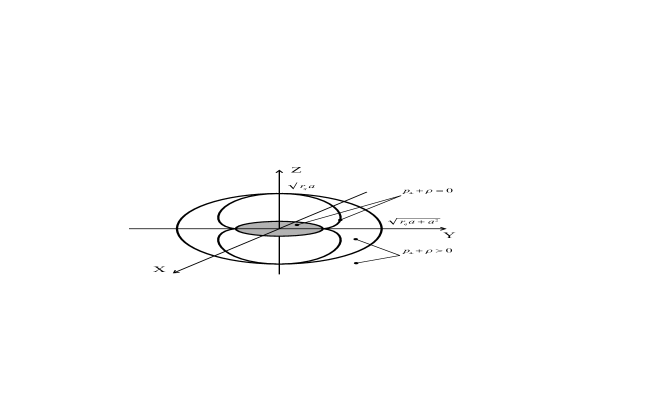
Figure 2: Vacuum ${\cal E}$-surface for the case $\alpha<\pi\beta^{2}/8$.

In the case $\alpha>\pi\beta^{2}/8$, the ${\cal E}$-surface is oblate (Fig. 3). It is the case for electromagnetic spinning soliton. It can be also the case of a slightly charged rotating black hole and of an extreme black hole.

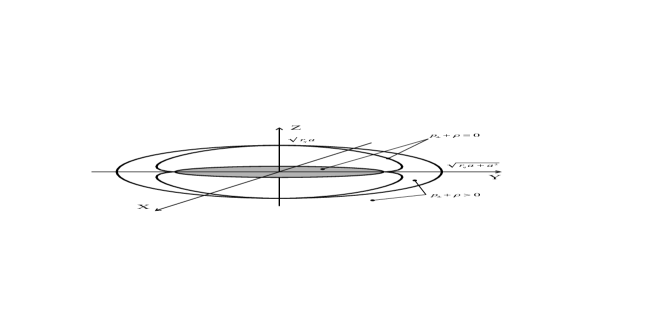
Figure 3: Vacuum ${\cal E}$-surface for the case $\alpha>\pi\beta^{2}/8$.

4 Electromagnetic fields

4.1 Field equations

Non-zero field components compatible with the axial symmetry are $F_{01},F_{02},F_{13},F_{23}$. In geometry with the metric (14) they are related by

$$F_{31}=a\sin^{2}\theta F_{10};~{}~{}aF_{23}=(r^{2}+a^{2})F_{02}.$$ (33)

The field invariant $F=F_{\mu\nu}F^{\mu\nu}$ in the axially symmetric case reduces to

$$F=2\left(\frac{F_{20}^{2}}{a^{2}\sin^{2}\theta}-F_{10}^{2}\right).$$ (34)

In terms of the 3-vectors, denoted by the italic indices running from 1 to 3 and defined as

$${E}_{j}=\{F_{j0}\};~{}~{}{D}^{j}=\{{\cal L}_{F}F^{0j}\};~{}~{}{B}^{j}=\{{{}^{*}}F^{j0}\};~{}~{}{H}_{j}=\{{\cal L}_{F}{{}^{*}}F_{0j}\},$$ (35)

the field equations (5)-(6) take the form of the source-free Maxwell equations

$$\nabla{\mathbf{D}}=0;~{}~{}\nabla\times{\mathbf{H}}=\frac{\partial{\mathbf{D}}}{\partial t};~{}~{}~{}\nabla{\mathbf{B}}=0;~{}~{}\nabla\times{\mathbf{E}}=-\frac{\partial{\mathbf{B}}}{\partial t}.$$ (36)

The electric induction ${\mathbf{D}}$ and the magnetic induction $\mathbf{B}$ are related with the electric and magnetic field intensities by

$$D^{j}=\epsilon^{j}_{k}E^{k};~{}~{}B^{j}=\mu^{j}_{k}H^{k},$$ (37)

where $\epsilon_{j}^{k}$ and $\mu_{j}^{k}$ are the tensors of the electric and magnetic permeability given by [22]

$$\epsilon_{r}^{r}=\frac{(r^{2}+a^{2})}{\Delta}{\cal L}_{F};~{}~{}\epsilon_{\theta}^{\theta}={\cal L}_{F};~{}~{}\mu_{r}^{r}=\frac{(r^{2}+a^{2})}{\Delta{\cal L}_{F}};~{}~{}\mu_{\theta}^{\theta}=\frac{1}{{\cal L}_{F}}.$$ (38)

Equations (5) and (6) form the system

$$\frac{\partial}{\partial r}[(r^{2}+a^{2})\sin\theta{\cal L}_{F}F_{10}]+\frac{\partial}{\partial\theta}[\sin\theta{\cal L}_{F}F_{20}]=0$$ (39)

$$\frac{\partial}{\partial r}\left[\frac{1}{\sin\theta}{\cal L}_{F}F_{31}\right]+\frac{\partial}{\partial\theta}\left[\frac{1}{(r^{2}+a^{2})\sin\theta}{\cal L}_{F}F_{32}\right]=0$$ (40)

$$\frac{\partial F_{23}}{\partial r}+\frac{\partial F_{31}}{\partial\theta}=0$$ (41)

$$\frac{\partial F_{01}}{\partial\theta}+\frac{\partial F_{20}}{\partial r}=0.$$ (42)

Four field components are related by two equations (33), so only two are independent and we can apply (33) to transform this system to the form

$$\frac{\partial}{\partial r}\biggl{[}(r^{2}+a^{2})\sin\theta{\cal L}_{F}F_{10}\biggr{]}+\frac{\partial}{\partial\theta}\biggl{[}\sin\theta{\cal L}_{F}F_{20}\biggr{]}=0$$ (43)

$$\frac{\partial}{\partial r}\biggl{[}a\sin\theta{\cal L}_{F}F_{10}\biggr{]}+\frac{\partial}{\partial\theta}\biggl{[}\frac{1}{a\sin\theta}{\cal L}_{F}F_{20}\biggr{]}=0$$ (44)

$$\frac{\partial}{\partial r}F_{20}-\frac{\partial}{\partial\theta}F_{10}=0$$ (45)

$$\frac{\partial}{\partial\theta}\biggl{[}a^{2}\sin^{2}\theta F_{10}\biggr{]}-\frac{\partial}{\partial r}\biggl{[}(r^{2}+a^{2})F_{20}\biggr{]}=0.$$ (46)

For calculation of derivatives in (43)-(44) we need derivatives of the invariant $F$ which read

$$\frac{\partial F}{\partial r}=4\biggl{(}\frac{F_{20}}{a^{2}\sin^{2}\theta}\frac{\partial F_{20}}{\partial r}-F_{10}\frac{\partial F_{10}}{\partial r}\biggr{)}$$ (47)

$$\frac{\partial F}{\partial\theta}=4\biggl{(}\frac{F_{20}}{a^{2}\sin^{2}\theta}\frac{\partial F_{20}}{\partial\theta}-\frac{\cot\theta}{a^{2}\sin^{2}\theta}F_{20}^{2}-F_{10}\frac{\partial F_{10}}{\partial\theta}\biggr{)}.$$ (48)

With taking into account (47), (48) and (45), we reduce the system (43)-(46) to

$$(r^{2}+a^{2})\biggl{\{}{\cal L}_{F}-4{\cal L}_{FF}F_{10}^{2}\biggr{\}}\frac{\partial F_{10}}{\partial r}+\biggl{\{}{\cal L}_{F}+4{\cal L}_{FF}\frac{F_{20}^{2}}{a^{2}\sin^{2}\theta}\biggr{\}}\frac{\partial F_{20}}{\partial\theta}$$

$$+4{\cal L}_{FF}\Sigma\frac{F_{10}F_{20}}{a^{2}\sin^{2}\theta}\frac{\partial F_{20}}{\partial r}+2r{\cal L}_{F}F_{10}+F_{20}\cot\theta\biggl{\{}{\cal L}_{F}-4{\cal L}_{FF}\frac{F_{20}^{2}}{a^{2}\sin^{2}\theta}\biggr{\}}=0$$ (49)

$$\biggl{\{}{\cal L}_{F}-4{\cal L}_{FF}F_{10}^{2}\biggr{\}}\frac{\partial F_{10}}{\partial r}+\frac{1}{a^{2}\sin^{2}\theta}\biggl{\{}{\cal L}_{F}+4{\cal L}_{FF}\frac{F_{20}^{2}}{a^{2}\sin^{2}\theta}\biggr{\}}\frac{\partial F_{20}}{\partial\theta}-\frac{\cot\theta}{a^{2}\sin^{2}\theta}F_{20}\biggl{\{}{\cal L}_{F}+4{\cal L}_{FF}\frac{F_{20}^{2}}{a^{2}\sin^{2}\theta}\biggr{\}}=0$$ (50)

$$\Sigma\frac{\partial F_{20}}{\partial r}+2rF_{20}-a^{2}\sin{2\theta}F_{10}=0$$ (51)

$$\frac{\partial}{\partial r}F_{20}-\frac{\partial}{\partial\theta}F_{10}=0.$$ (52)

Two of these equations are strongly non-linear.

4.2 Asymptotic solutions

Dynamical equations $\nabla_{\mu}({\cal L}_{F}F^{\mu\nu})=0$ are satisfied by the functions [22]

$$\Sigma^{2}({\cal L}_{F}F_{01})=-q(r^{2}-a^{2}\cos^{2}\theta);~{}~{}\Sigma^{2}({\cal L}_{F}F_{02})=qa^{2}r\sin 2\theta;$$ (53)

$$\Sigma^{2}({\cal L}_{F}F_{31})=aq\sin^{2}\theta(r^{2}-a^{2}\cos^{2}\theta);~{}~{}~{}\Sigma^{2}({\cal L}_{F}F_{23})=aqr(r^{2}+a^{2})\sin 2\theta.$$ (54)

In the case ${\cal L}_{F}=1$, they satisfies also the dynamical equations (6) and coincide with the solutions to the Maxwell-Einstein equations [3, 12].

The field functions (54)-(53) satisfy the equations

$$\frac{\partial({\cal L}_{F}F_{23})}{\partial r}+\frac{\partial({\cal L}_{F}F_{31})}{\partial\theta}=0$$ (55)

$$\frac{\partial({\cal L}_{F}F_{01})}{\partial\theta}+\frac{\partial({\cal L}_{F}F_{20})}{\partial r}=0.$$ (56)

It follows

$$\frac{\partial F_{23}}{\partial r}+\frac{\partial F_{31}}{\partial\theta}=-\frac{{\cal L}_{FF}}{{\cal L}_{F}}\left[F_{31}\frac{\partial F}{\partial\theta}+F_{23}\frac{\partial F}{\partial r}\right]$$ (57)

$$\frac{\partial F_{01}}{\partial\theta}+\frac{\partial F_{20}}{\partial r}=-\frac{{\cal L}_{FF}}{{\cal L}_{F}}\left[F_{01}\frac{\partial F}{\partial\theta}+F_{20}\frac{\partial F}{\partial r}\right]$$ (58)

Left sides vanish identically when right sides are zero. This defines the following cases when the functions (54)-(53) satisfy the dynamical system (39)-(42):

(A) ${\cal L}_{FF}=0,{\cal L}_{F}\neq 0$, the case of the linear electromagnetic field;

(B) ${\cal L}_{F}=\infty,{\cal L}_{FF}\neq 0$, strongly nonlinear regime. Density of electromagnetic energy given by (20) grows towards the interior disk $r=0$. Applying (54)-(53) we obtain

$$\kappa{(p_{\perp}+\rho)}=\frac{2q^{2}}{{\cal L}_{F}\Sigma^{2}}.$$ (59)

For the regular solutions on the interior disk geometry requires $p_{\perp}+\rho=0$. It follows ${\cal L}_{F}\Sigma^{2}\rightarrow\infty$ and hence ${\cal L}_{F}\rightarrow\infty$, since $\Sigma\rightarrow 0$ on the disk. The case (B) represents thus realization of the underlying hypothesis of non-linearity replacing a singularity.

Third possibility is vanishing of the expression in the square brackets in the right hand sides of equations (57)-(58)

$$F_{31}\frac{\partial F}{\partial\theta}+F_{23}\frac{\partial F}{\partial r}=0$$ (60)

$$F_{01}\frac{\partial F}{\partial\theta}+F_{20}\frac{\partial F}{\partial r}=0.$$ (61)

With taking into account (33), this system reduces to

$$a^{2}\sin^{2}\theta F_{01}\frac{\partial F}{\partial\theta}+(r^{2}+a^{2})F_{20}\frac{\partial F}{\partial r}=0$$ (62)

$$F_{01}\frac{\partial F}{\partial\theta}+F_{20}\frac{\partial F}{\partial r}=0.$$ (63)

It is the system of two algebraic equations for $F_{01}({\partial F}/{\partial\theta})$ and $F_{20}({\partial F}/{\partial r})$. Its determinant is equal $Det=-\Sigma$. The case $\Sigma\neq 0$ corresponds to the trivial solutions $F_{01}({\partial F}/{\partial\theta})=0$, $F_{20}({\partial F}/{\partial r})=0$, and includes the case

(C) $F_{10}=F_{20}=0$, zero fields regime.

4.3 Necessary condition for the existence of solutions

The basic question in the case of the system of four equations (39)-(42) for three functions $F_{10},F_{20}$ and ${\cal L}_{F}$, is the question of its compatibility, i.e. compatibility of equations (5)-(6).

The system (39)-(42) for $F_{10},F_{20}$ and ${\cal L}_{F}$, with taking into account (33), reduces to

$$(r^{2}+a^{2})\frac{\partial F_{10}}{\partial r}+\frac{\partial F_{20}}{\partial\theta}=A_{1}F_{10}+A_{2}F_{20}$$ (64)

$$\frac{\partial F_{10}}{\partial r}+\frac{1}{a^{2}\sin^{2}\theta}\frac{\partial F_{20}}{\partial\theta}=B_{1}F_{10}+B_{2}F_{20}$$ (65)

$$\sin^{2}\theta\frac{\partial F_{10}}{\partial\theta}-\frac{(r^{2}+a^{2})}{a^{2}}\frac{\partial F_{20}}{\partial r}=C_{1}F_{10}+C_{2}F_{20}$$ (66)

$$-\frac{\partial F_{10}}{\partial\theta}+\frac{\partial F_{20}}{\partial r}=0,$$ (67)

where

$$A_{1}=-2r-(r^{2}+a^{2})\frac{1}{{\cal L}_{F}}\frac{\partial{\cal L}_{F}}{\partial r};~{}~{}~{}A_{2}=-\cot\theta-\frac{1}{{\cal L}_{F}}\frac{\partial{\cal L}_{F}}{\partial\theta};~{}~{}~{}B_{1}=-\frac{1}{{\cal L}_{F}}\frac{\partial{\cal L}_{F}}{\partial r};$$ (68)

$$B_{2}=\frac{\cos\theta}{a^{2}\sin^{3}\theta}-\frac{1}{a^{2}\sin^{2}\theta}\frac{1}{{\cal L}_{F}}\frac{\partial{\cal L}_{F}}{\partial\theta};~{}~{}~{}C_{1}=-\sin 2\theta;~{}~{}~{}C_{2}=\frac{2r}{a^{2}}.$$ (69)

The system (64)-(67) can be resolved with respect to the derivatives of $F_{10}$ and $F_{20}$. This gives

$$\frac{\partial F_{10}}{\partial r}={\tilde{A}}_{1}F_{10}+{\tilde{A}}_{2}F_{20}$$ (70)

$$\frac{\partial F_{20}}{\partial\theta}={\tilde{B}}_{1}F_{10}+{\tilde{B}}_{2}F_{20}$$ (71)

$$\frac{\partial F_{10}}{\partial\theta}=\frac{\partial F_{20}}{\partial r}={\tilde{C}}_{1}F_{10}+{\tilde{C}}_{2}F_{20},$$ (72)

where

$${\tilde{A}}_{1}=-\frac{2r}{\Sigma}-\frac{1}{{\cal L}_{F}}\frac{\partial{\cal L}_{F}}{\partial r};~{}~{}~{}{\tilde{A}}_{2}=-\frac{2\cot\theta}{\Sigma};~{}~{}~{}{\tilde{B}}_{1}=\frac{2a^{2}r\sin^{2}\theta}{\Sigma}~{};$$ (73)

$${\tilde{B}}_{2}=\frac{1}{\Sigma}\bigg{[}\cot\theta\bigg{(}r^{2}+a^{2}+a^{2}\sin^{2}\theta\bigg{)}\bigg{]}-\frac{1}{{\cal L}_{F}}\frac{\partial{\cal L}_{F}}{\partial\theta};~{}~{}~{}{\tilde{C}}_{1}=\frac{a^{2}\sin 2\theta}{\Sigma};~{}~{}~{}{\tilde{C}}_{2}=-\frac{2r}{\Sigma}.$$ (74)

Equality of the mixed second derivatives of $F_{10}$ and $F_{20}$ gives, respectively,

$$D_{1}F_{10}+D_{2}F_{20}=0,~{}~{}D_{3}F_{10}+D_{4}F_{20}=0,$$ (75)

where

$$D_{1}=-\frac{\partial}{\partial\theta}\bigg{(}\frac{1}{{\cal L}_{F}}\frac{\partial{\cal L}_{F}}{\partial r}\bigg{)};~{}~{}~{}D_{2}=\frac{2}{\Sigma{\cal L}_{F}}\bigg{[}r\frac{\partial{\cal L}_{F}}{\partial r}+\cot\theta\frac{\partial{\cal L}_{F}}{\partial\theta}\bigg{]};$$ (76)

$$D_{3}=\frac{2a^{2}\sin^{2}\theta}{\Sigma{\cal L}_{F}}\bigg{[}r\frac{\partial{\cal L}_{F}}{\partial r}+\cot\theta\frac{\partial{\cal L}_{F}}{\partial\theta}\bigg{]};~{}~{}~{}D_{4}=\frac{\partial}{\partial r}\bigg{(}\frac{1}{{\cal L}_{F}}\frac{\partial{\cal L}_{F}}{\partial\theta}\bigg{)}.$$ (77)

We obtained the uniform system of two algebraic equations (75) with respect to field tensions $F_{10}$ and $F_{20}$. Necessary and sufficient condition of the existence of a non-trivial solution of this system is vanishing of its determinant. Hence, the necessary and sufficient condition of compatibility of equations (64)-(67) is

$$D_{1}D_{4}-D_{2}D_{3}=0.$$ (78)

In the explicit form it reads

$$\frac{\partial}{\partial r}\bigg{(}\frac{1}{L_{F}}\frac{\partial L_{F}}{\partial\theta}\bigg{)}\frac{\partial}{\partial\theta}\bigg{(}\frac{1}{L_{F}}\frac{\partial L_{F}}{\partial r}\bigg{)}+\frac{4a^{2}\sin^{2}(\theta)}{\Sigma^{2}}\frac{1}{L^{2}_{F}}\bigg{[}r\frac{\partial L_{F}}{\partial r}+\cot(\theta)\frac{\partial L_{F}}{\partial\theta}\bigg{]}^{2}=0.$$ (79)

This is the condition on a function ${\cal L}_{F}$, which is the necessary and sufficient condition of compatibility of equations (5)-(6) and hence necessary condition for the existence of solutions.

The condition (79) is evidently satisfied for ${\cal L}_{F}=$const which can be normalized to ${\cal L}_{F}=1$ and corresponds to the Maxwell weak field limit, and in the case of trivial zero fields solutions.

The equation (79) can be written as

$$\frac{1}{{\cal L}_{F}^{2}}\bigg{(}\frac{\partial^{2}{\cal L}_{F}}{\partial r\partial\theta}\bigg{)}^{2}-\frac{{\cal L}_{FF}}{{\cal L}_{F}^{3}}\bigg{(}\frac{\partial^{2}{\cal L}_{F}}{\partial r\partial\theta}\bigg{)}^{2}\bigg{[}\frac{\partial F}{\partial\theta}\frac{\partial{\cal L}_{F}}{\partial r}+\frac{\partial F}{\partial r}\frac{\partial{\cal L}_{F}}{\partial\theta}\bigg{]}+\frac{4a^{2}\sin^{2}(\theta)}{\Sigma^{2}}\frac{1}{L^{2}_{F}}\bigg{[}r\frac{\partial L_{F}}{\partial r}+\cot(\theta)\frac{\partial L_{F}}{\partial\theta}\bigg{]}^{2}=0.$$ (80)

This condition should be analyzed carefully since it implies that ${\cal L}_{F}(r,\theta)\subset C^{2}$. However, it could be not the case on the whole manifold. For regular solutions, invariant $F$ vanishes on the disk where it is given by [22]

$$F=-\frac{\kappa^{2}(p_{\perp}+\rho)^{2}\Sigma^{2}}{2q^{2}},$$ (81)

and vanishes at infinity in the Maxwell weak field limit. Lagrangian ${\cal L}(F)$ is a function of a non-monotonic function $F$ with equal limiting values and should suffer branching and have a cusp at a certain value of $F$. Correct description of Lagrange dynamics requires non-uniform variational problem [37]. On the boundary hypersurface which divides two regions of the manifold with different Lagrangians, the function ${\cal L}_{F}$ does not belong to the class $C^{2}$ as a function of $F$, but can be $C^{2}$ as a function of $r$ and $\theta$. This point has been studied separately and the results will be reported somewhere [43]. Here we point out that ${\cal L}_{F}$ is finite in the boundary region and is $C^{2}$ in the region described by the internal Lagrangian including the interior region where ${\cal L}_{F}\rightarrow\infty$. In this region asymptotic solutions (54)-(53) satisfy dynamical equations (5)-(6), regularity requires ${\cal L}_{F}\Sigma^{2}\rightarrow\infty$ and ${\cal L}_{F}\rightarrow\infty$, so that the condition (80) is satisfied and gives formal confirmation of compatibility of the system (5)-(6) in this limit.

5 Vacuum interiors

The relation connecting density and pressure with the electromagnetic fields reads [22]

$$\kappa(p_{\perp}+\rho)=2{\cal L}_{F}\left(F_{10}^{2}+\frac{F_{20}^{2}}{a^{2}\sin^{2}\theta}\right).$$ (82)

Vacuum ${\cal E}$-surface is defined by $p_{\perp}+\rho=0$. By virtue of (59) it leads to ${\cal L}_{F}\rightarrow\infty$. As a result the magnetic permeability vanishes and electric permeability goes to infinity, so that the ${\cal E}$-surface and the disk display the properties of a perfect conductor and ideal diamagnetic. In the limit ${\cal L}_{F}\rightarrow\infty$ the magnetic induction vanishes on the vacuum ${\cal E}$-surface and on the disk by virtue of the asymptotic solutions (53) which satisfy the dynamical equations (5)-(6) in this limit.

On the de Sitter disk $r=0$ we obtain from (37)-(38) $\epsilon_{r}^{r}=\epsilon_{\theta}^{\theta}={\cal L}_{F}$ and $\mu_{r}^{r}=\mu_{\theta}^{\theta}={{\cal L}_{F}}^{-1}=\mu\rightarrow 0$. The magnetic induction $\mathbf{B}$ also vanishes on the disk. In electrodynamics of continued media the transition to a superconducting state corresponds to the limits ${\mathbf{B}}\rightarrow 0$ and $\mu\rightarrow 0$ in a surface current ${\mathbf{j_{s}}}=\frac{(1-\mu)}{4\pi\mu}[{\mathbf{n}}{\mathbf{B}}]$, where ${\mathbf{n}}$ is the normal to the surface. The right-hand side then becomes indeterminate, and there is no condition which would restrict the possible values of the current [39]. On the de Sitter disk we can apply definition of a surface current for a charged surface layer, $4\pi j_{k}=[e_{(k)}^{\alpha}F_{\alpha\beta}n^{\beta}]$ [4], where $[..]$ denotes a jump across the layer; $e_{(k)}^{\alpha}$ are the tangential base vectors associated with the intrinsic coordinates on the disk $t,\phi$, $0\leq\xi\leq\pi/2$; $n_{\alpha}=(1+q^{2}/a^{2})^{-1/2}\cos\xi~{}\delta^{1}_{\alpha}$ is the unit normal directed upwards [4]. With using asymptotic solutions (53) and magnetic permeability $\mu=1/{\cal L}_{F}$, we obtain the surface current [32]

$$j_{\phi}=-\frac{q}{2\pi a}~{}\sqrt{1+q^{2}/a^{2}}~{}\sin^{2}\xi~{}\frac{\mu}{\cos^{3}\xi}.$$ (83)

At approaching the ring $r=0,~{}\xi=\pi/2$, both terms in the second fraction go to zero quite independently. As a result the surface currents on the ring can be any and amount to a non-zero total value. Superconducting currents flowing (forever) on the de Sitter vacuum ring can be considered as a source of the Kerr-Newman fields. This kind of a source is non-dissipative so that life time of the electromagnetic spinning structure can be unlimited.

We find the existence of the interior de Sitter vacuum ${\cal E}$-surface, which contains de Sitter disk as the bridge, with zero magnetic induction on the whole surface. The next question - what is going on within ${\cal E}$-surface, in cavities between its upper and down boundaries and the bridge? Negative value of $(p_{\perp}+\rho)$ in (82)  would mean negative values for the electric and magnetic permeabilities inadmissible in electrodynamics of continued media [39].

One possibility to satisfy the basic requirement of electrodynamics of continued media, can be zero value of $(p_{\perp}+\rho)$ also inside ${\cal E}$-surface. This can be the case for the shell-like models ([9] and references therein) with the flat vacuum interior, zero fields and in consequence zero density and pressures, and no violation of the weak energy condition.

The other possibility, favored by the underlying idea of nonlinearity replacing a singularity and suggested by vanishing of magnetic induction on the surrounding ${\cal E}$-surface, is the extension of ${\cal L}_{F}\rightarrow\infty$ to its interiors. Then we have de Sitter vacuum core, $p=-\rho$, with the properties of a perfect conductor and ideal diamagnetic, zero magnetic induction, and valid weak energy condition throughout the whole core.

6 Summary and discussion

We studied regular rotating electrically charged rotating black holes and solitons in nonlinear electrodynamics non-minimally coupled to gravity with the model-independent approach based on generic information following from the source-free dynamical equations, in which nonlinear electromagnetic fields provide a source in the Einstein equations.

Regular spherically symmetric NED-GR solutions are asymptotically de Sitter for $r\rightarrow 0$ and asymptotically Reissner-Nordström for $r\rightarrow\infty$. They always satisfy the weak energy condition since $\kappa(p_{\perp}+\rho)=-{\cal L}_{F}F$, the invariant $F$ is generically non-positive and ${\cal L}_{F}$ represents the electric permeability which can not be negative in electrodynamics of continued media.

The spherical solutions give rise, by the Gürses-Gürsey algorithm, to regular axially symmetric solutions describing rotating electrically charged black holes and solitons, asymptotically Kerr-Newman for a distant observer. Black holes have at most two horizons and ergoregions. Solitons can have two ergoregions.

We formulated the necessary and sufficient conditions of compatibility of dynamical equations governing the electromagnetic fields dynamics, necessary for the existence of solutions, and found asymptotic solutions needed to study field dynamics in the interior regions.

Rotation transforms de Sitter center into de Sitter disk $r=0$ with $p_{\perp}+\rho=0$ and with superconducting current flowing on the surrounding ring (in place of the Kerr singularity). Superconducting current can be regarded as a non-dissipative source of the Kerr-Newman exterior fields, providing unlimited life time of NED-GR spinning regular objects [32].

The weak energy condition could be violated in the case when the related spherical solution satisfies the dominant energy condition. In this case there exists the vacuum ${\cal E}$-surface defined by $p_{\perp}+\rho=0$ with the de Sitter disk $r=0$ as a bridge. Both ${\cal E}$-surface and the disk have properties of the perfect conductor and ideal diamagnetic. Violation of the weak energy condition inside the vacuum surface would need negative values of electric and magnetic permeability inadmissible in electrodynamics of continued media. We can conclude that WEC is not violated in the interiors of regular rotating charged black holes and solitons in NED-GR theories compatible with the basic requirement of electrodynamics of continued media on the electric and magnetic permeability.

Alternative favored by the underlying idea of non-linearity regularizing a singularity and suggested by vanishing magnetic induction on the vacuum ${\cal E}$-surface, is extension of its basic properties to its interior. Then the regular interior is presented by de Sitter vacuum core with properties of perfect conductor and ideal diamagnetic.

This work was motivated by search for an image of the electron, inspired by the Dirac paper on the extended electron [44], and by the Carter remarkable discovery of ability of the Kerr-Newman solution to represent the electron for a distant observer. Electromagnetic spinning soliton can be considered as the Coleman lump, a non-singular, non-dissipative solution of finite energy holding itself together by its own self-interaction [45], which can be applied as the model for the extended electron.

For the electron $q=-e$ and $a=\lambda/2$ where $\lambda=\hbar/m$ is its Compton wavelength [3]. In the observer region $r\gg\lambda_{e}$

$$E_{r}=-\frac{e}{r^{2}}\left(1-\frac{\hbar^{2}}{m_{e}^{2}c^{2}}\frac{3\cos^{2}\theta}{4r^{2}}\right);~{}E_{\theta}=\frac{e\hbar^{2}}{m_{e}^{2}c^{2}}\frac{\sin 2\theta}{4r^{3}};~{}~{}B^{r}=-\frac{e\hbar}{m_{e}c}\frac{\cos\theta}{r^{3}}=2\mu_{e}\frac{\cos\theta}{r^{3}};~{}B_{\theta}=-\mu_{e}\frac{\sin\theta}{r^{4}}.$$ (84)

The Planck constant appears due to discovered by Carter ability of the Kerr-Newman solution to present the electron as seen by a distant observer. In terms of the Coleman lump (84) describes the following situation: The leading term in $E_{r}$ gives the Coulomb law as the classical limit $\hbar=0$, and the higher terms represent the quantum corrections.

Purely electromagnetic reaction of annihilation $e^{+}e^{-}\rightarrow\gamma\gamma(\gamma)$ reveals, at the $5\sigma$ confidence level, the existence of the minimal length $l_{e}=1.57\times 10^{-17}$ cm at the scale $E=1.253$ TeV which can be explained as the distance of the closest approach of annihilating particles where electromagnetic attraction is stopped by the gravitational repulsion of the interior de Sitter vacuum of electromagnetic spinning soliton [46].

References

- [1] E.T. Newman, E. Cough, K. Chinnapared, A. Exton, A. Prakash, and R. Torrence, J. Math. Phys. 6 (1965) 918.
- [2] E.T. Newman and A.J. Janis, J. Math. Phys. 6 (1965) 915.
- [3] B. Carter, Phys. Rev. 174 (1968) 1559.
- [4] W. Israel, Phys. Rev. D 2 (1970) 641.
- [5] A.Ya. Burinskii, Sov. Phys. JETP 39 (1974) 193.
- [6] C.A. López, Nuovo Cim. 76 B (1983) 9.
- [7] V. de la Cruz, J.E. Chase, and W. Israel, Phys. Rev. Lett. 24 (1970) 423.
- [8] J.M. Cohen, J. Math. Phys. 8 (1967) 1477.
- [9] C.A. López, Phys. Rev. D 30 (1984) 313.
- [10] R.H. Boyer, Proc. Cambridge Phil. Soc. 61 (1965) 527; ibid, 62 (1966) 495.
- [11] M. Trümper, Z. Naturforschung 22a (1967) 1347.
- [12] J. Tiomno, Phys. Rev. D 7 (1973) 992.
- [13] A.Ya. Burinskii, Phys. Lett. B 216 (1989) 123.
- [14] A. Burinskii, Grav. and Cosmology 8 (2002) 261.
- [15] A. Burinskii, E. Elizalde, S.R. Hildebrandt, G. Magli, Phys. Rev. D 65 (2002) 064039.
- [16] A. Burinskii, Int. J. Mod. Phys. A 29 (2014) 1450133.
- [17] A. Burinskii, Theor. Math. Phys. 177 (2013) 1492.
- [18] E.S. Fradkin and A.A. Tseytlin, Phys. Lett. B 163 (1985) 123.
- [19] A.A. Tseytlin, Nucl. Phys. B 276 (1986) 391.
- [20] N. Siberg and E. Witten, JHEP vol.1999, article 032 (1999).
- [21] M. Born and L. Infeld, Proc. R. Soc. London A 144 (1934) 425.
- [22] I. Dymnikova, Phys. Lett. B 639 (2006) 368.
- [23] I. Dymnikova, Gen. Rel. Grav. 24 (1992) 235.
- [24] I. Dymnikova, Phys. Lett. B 472 (2000) 33.
- [25] I. Dymnikova, Class. Quant. Grav. 19 (2002) 725.
- [26] I. Dymnikova, Int. J. Mod. Phys. D 12 (2003) 1015.
- [27] I. Dymnikova, Class. Quant. Grav. 21 (2004) 4417.
- [28] R.P. Kerr and A. Schild, Proc. of Symp. in Appl. Math. 17 (1965) 199.
- [29] E. Elizalde and S.R. Hildebrandt, Phys. Rev. D 65 (2002) 124024.
- [30] M. Gürses and F. Gürsey, J. Math. Phys. 16 (1975) 2385.
- [31] A. Burinskii and S.R. Hildebrandt, Phys. Rev. D 65 (2002) 104017.
- [32] I. Dymnikova, to be published (2015).
- [33] C. Bambi, L. Modesto, Phys. Lett. B 721 (2013) 329.
- [34] J.C.S. Neves and A. Saa, Phys. Lett. B 734 (2014) 44.
- [35] B. Toshmatov, B. Ahmedov, A. Abdujabbarov, and Z. Stuchlik, Phys. Rev. D 89 (2014) 104017.
- [36] K.A. Bronnikov, Phys. Rev. D 63 (2001) 044005.
- [37] I. Dymnikova, E. Galaktionov, and E. Tropp, Advances in Math. Phys. Volume 2015, Article ID 496475 (2015).
- [38] S. Chandrasekhar, The Mathematical Theory of Black Holes, Clarendon Press (1983).
- [39] L.D. Landau and E.M. Lifshitz Electrodynamics of Continued Media, Pergamon Press (1993).
- [40] I. Dymnikova and Galaktionov (2015), to be published.
- [41] M.Zilho, V.Cardoso, C.Herdeira, L.Lehner, U.Sperhake, Phys. Rev. D 89 (2014) 044008.
- [42] A.J.S. Hamilton, Phys. Rev. D 84 (2011) 124057.
- [43] I. Dymnikova, E. Galaktionov, and E. Tropp (2015), to be published.
- [44] P.A.M. Dirac, Proc. Roy. Soc. Lond. A 268 (1962) 57.
- [45] S. Coleman, in: New Phenomena in Subnuclear Physics, Ed. A. Zichichi, New York: Plenum (1977) 297.
- [46] I. Dymnikova, A. Sakharov and J. Ulbricht, AHEP vol. 2014, ID 707812 (2014).