Stochastic model for phonemes uncovers an author-dependency of their usage

Abstract

We study rank-frequency relations for phonemes, the minimal units that still relate to linguistic meaning. We show that these relations can be described by the Dirichlet distribution, a direct analogue of the ideal-gas model in statistical mechanics. This description allows us to demonstrate that the rank-frequency relations for phonemes of a text do depend on its author. The author-dependency effect is not caused by the author's vocabulary (common words used in different texts), and is confirmed by several alternative means. This suggests that it can be directly related to phonemes. These features contrast to rank-frequency relations for words, which are both author and text independent and are governed by the Zipf's law.

I Introduction

Language can be viewed as a hierarchic construction: phoneme, syllable, morpheme, word … Each of these objects expresses meaning or participates in its formation, and consists of elements of the previous level, i.e. syllable consists of phonemes scherba ; phoneme_def ; sapir .

The lowest hierarchic level is phoneme, which is defined to be a representative for a group of sounds that are not distinguishable with respect to their meaning-formation function in a concrete language. For instance /r/ and /l/ are different phonemes in English, e.g. because row and low which differ only by these phonemes are different words; see section I of the supplementary material for a list of English phonemes. But they are the same phoneme in Japanese, since in that language there is no danger of meaning-ambiguity upon mixing /r/ with /l/. (Different speech sounds that are realizations of the same phoneme are known as allophones.) Thus the meaning is crucial for the definition of the phoneme, although a single phoneme does not express a separate meaning scherba ; phoneme_def ; sapir . The next hierarchic level (syllable) indirectly participates in the definition of the phoneme, since the syllable bounds phonemes, i.e. there cannot be a phoneme which belongs to two different syllables; e.g. diphthongs belong to the same syllable scherba ; phoneme_def .

The history of phoneme is a rich and complex one. It appeared in Greek and Indian linguistic traditions simultaneously with atomistic ideas in natural philosophy skoyles ; staal ; lysenko . Analogies between atom and phoneme are still potent in describing complex systems zwick ; abler . Within the Western linguistic tradition the development of phoneme was for a while overshadowed by related (but different) concepts of letter and sound scherba ; phoneme_def . The modern definition of phoneme goes back to late XIX century phoneme_def . While it is agreed that the phoneme is a unit of linguistic analysis sapir , its psychological status is a convoluted issue port ; suomi ; nathan ; savin ; foss . Different schools of phonology and psychology argue differently about it, and there is a spectrum of opinions concerning the issue (e.g. perception of phonemes, their identification, reproduction etc) savin ; foss ; see port ; suomi ; nathan for recent reviews.

For defining a rank-frequency relation, one calculates the frequencies $f_{r}$ of certain constituents (e.g. words or phonemes) entering into a given text, lists them in a decreasing order

$$f_{1}\geq f_{2}\geq...\geq f_{n},$$ (1)

and studies the dependence of the frequency $f_{r}$ on the rank $r$ (its position in (1), $1\leq r\leq n$). This provides a coarse-grained description, because not the frequencies of specific phonemes are described, but rather the order relation between them, e.g. the same form of the rank-frequency relation in two different texts is consistent with the same phoneme having different frequencies in those texts. The main point of employing rank-frequency relations is that they (in contrast to the full set of frequencies) can be described via simple statistical models with very few parameters.

Rank-frequency relations are well-known for words, where they comply to the Zipf's law; see wyllis ; baa for reviews. This law is universal in the sense that for all sufficiently long texts (and their mixtures, i.e. corpora) it predicts the same power law shape $f_{r}\propto r^{-1}$ for the dependence of the word frequency on its rank. It was shown recently that the representation of the word frequencies via hidden frequencies|the same idea as employed in the present work|is capable of reproducing both the Zipf's law and its generalizations to low-frequency words (hapax legomena) zipf_pre . Due to its universality, the Zipf's law for words cannot relate the text to its author.

The rank-frequency relation for morphemes and syllables was so far not studied systematically. Ref. zipf_chin comes close to this potentially interesting problem, since it studies the rank-frequency relations of Chinese characters, which are known to represent both morpheme and syllable (in this context see also am_j ; sh ; chen_guo ). This study demonstrated that the Zipf's law still holds for a restricted range of ranks. For long texts this range is relatively small, but the frequencies in this range are important, since they carry out $\simeq 40$ % of the overall text frequency. It was argued that the characters in this range refer to the most polysemic morphemes zipf_chin .

There are also several works devoted to the rank-frequency relations of phonemes and letters sigurd ; good ; gusein_1 ; gusein_2 ; witten_bell ; tambov ; hindu . One of first works is that by Sigurd, who has shown that the phoneme rank-frequency relations are not described by the Zipf's law sigurd . He also noted that a geometric distribution gives a better fit than the Zipf's law. Other works studied various few-parameter functions|e.g. the Yule's distribution|and fitted it to the rank-frequency relations for phonemes of various languages; see hindu for a recent review of that activity.

The present work has two motivations. First, we want to provide an accurate description of rank-frequency relation for phonemes. It is shown that such a description is provided by postulating that phoneme frequencies are random variables with a given density. The ranked frequencies are then recovered via the order statistics of this density. This postulate allows to restrict the freedom of choosing various (theoretical) forms of rank-frequency relations, since|as developed in mathematical statistics neutral ; washington |the idea of the simplest density for probability of probability allows to come up with the unique family of Dirichlet densities. This family is characterized by a positive parameter $\beta$, which allows quantitative comparison between phoneme frequencies for different authors. From the physical side, the Dirichlet density is a direct analogue of the ideal gas model from statistical mechanics, while $\beta$ relates to the inverse temperature. Recall that the ideal-gas model provides a simple and fruitful description of the coarse-grained (thermodynamic) features of matter starting from the principles of atomic and molecular physics balian . Thus we substantiate the atom-phoneme metaphor, that so far was developed only qualitatively zwick ; abler .

Our second motivation for studying rank-frequency relations for phonemes is whether they can provide information on the author of the text, and thereby attempt at clarifying the psychological aspect of phonemes. As seen below, the Dirichlet density not only leads to an accurate description of phoneme rank-frequency relations, but it also allows to establish that the frequencies of phonemes do depend on the author of the text. We corroborate this result by an alternative means.

The closest to the present approach is the study by Good good which was developed in Refs. gusein_1 ; gusein_2 ; witten_bell . These authors applied the same idea on hidden probabilities as here, but they restricted themselves by the flat density, which is a particular case $\beta=1$ of the Dirichlet density good ; gusein_1 ; gusein_2 . Superficially, this case seems to be special, because it incorporates the idea of non-informative (unknown) probabilities (in the Bayesian sense) jaynes . However, the development of the Bayesian statistics has shown that the $\beta=1$ case of the Dirichlet density is by no means special with respect the prior information jaynes . Rather, the whole family of Dirichlet densities (with $\beta>0$ being a free parameter) qualifies for this role schafer .

This paper is organized as follows. Next section discusses the Dirichlet density and its features. There we also deduce explicit formulas for the probabilities ordered according to the Dirichlet density. Then, we analyze the data obtained from English texts written by different authors and show that it can be described via the Dirichlet density. There we also demonstrate (in different ways including non-parametric methods) that rank-frequency relations for phonemes are author-dependent. Next, we show that the author-dependency effect is not caused by common words used in different texts. We summarize in the last section.

II Dirichlet density

II.1 Ideal-gas models

The general idea of applying ideal-gas models in physics balian is that for describing coarse-grained features of certain physical systems, interactions between their constituents (atoms or molecules) can be accounted for superficially (in particular, neglected to a large extent). Instead, one focusses on the simplest statistical description that contains only a few parameters (e.g. temperature, volume, number of particles etc) balian . In physics this simplest descriptions amounts to the Gibbs density balian . Its analogue in mathematical statistics is known as the Dirichlet density, and is explained below. Ideal gas models in physics are useful not only for gases|where interactions are literally weak|but also for solids, where interactions are important, but their detailed structure is not, and hence it can be accounted for in a simplified way balian .

Following these lines, we apply below the Dirichlet density to phoneme frequencies observed in a given text. More precisely, the ordered frequencies generated by the Dirichlet density are compared with observed (and ordered) frequencies of phonemes in a given text. This ordering of frequencies amounts to a rough and simplified account of (inter-phoneme) interactions, and suffices for an accurate description of the rank-frequency relations for phonemes; see below.

II.2 Definition and main features

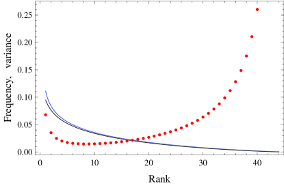
Figure 1: Rank-frequency curves and error generated by the Dirichlet density with $\beta=0.8$ and $n=44$. Blue curve: $\langle\theta_{(r)}\rangle$ (as a function of $r$) calculated according to (7–9). Black curve: $\hat{f}_{r}$ calculated via the approximate formula (10); cf. section II of the supplementary material. Red points: the normalized variance $(\langle\theta_{(r)}^{2}\rangle-\langle\theta_{(r)}\rangle^{2})/\langle\theta_{(r)}\rangle^{2}$ for $r=1,...,44$ calculated according to (7–9). This expression is well approximated by (39).

The Dirichlet density ${\cal D}(\theta_{1},...,\theta_{n})$ is a probability density over continuous variables $(\theta_{1},...,\theta_{n})$ which by themselves have the meaning of probabilities, i.e. ${\cal D}(\theta_{1},...,\theta_{n})$ is non-zero only for $\theta_{k}\geq 0$ and $\sum_{k=1}^{n}\theta_{k}=1$:

$${\cal D}(\theta_{1},...,\theta_{n}|\beta_{1},...,\beta_{n})=\frac{\Gamma[\sum_{k=1}^{n}\beta_{k}]}{\prod_{k=1}^{n}\Gamma[\beta_{k}]}\prod_{k=1}^{n}\theta_{k}^{\beta_{k}-1}\,\delta(\sum_{k=1}^{n}\theta_{k}-1),$$ (2)

where $\beta_{k}>0$ are the parameters of the Dirichlet density, $\delta(x)$ is the delta-function, $\Gamma[x]=\int_{0}^{\infty}{\rm d}\theta\,\theta^{x-1}e^{-\theta}$ is the Euler's $\Gamma$-function, and (2) is properly normalized: $\int_{0}^{\infty}\prod_{k=1}^{n}{\rm d}\theta_{k}{\cal D}(\theta_{1},...,\theta_{n}|\beta_{1},...,\beta_{n})=1$.

The random variables $\Theta_{1},...,\Theta_{n}$ (with realizations $\theta_{1},...,\theta_{n}$) are independent modulo the constraint that they sum to $1$; see (2). In this sense (2) is the simplest density for probabilities. Now (2) for a particular case $\beta_{k}=\beta$ (which is most relevant for our purposes) can be given the following statistical-physics interpretation: if $\ln(\frac{1}{\theta_{k}})$ is interpreted as the energy of $k$ shrejder ; dover ; vakarin , then $\beta-1$ becomes the inverse temperature for an ideal gas. It is useful to keep this analogy in mind, when discussing further features of the Dirichlet density.

Consider the subset $(\theta_{1},...,\theta_{m})$ ($m<n$) of probabilities $(\theta_{1},...,\theta_{n})$. If $(\theta_{1},...,\theta_{m})$ should serve as new probabilities, they should be properly normalized. Hence we define new random variables as follows:

$$(\widetilde{\theta}_{1},...,\widetilde{\theta}_{n})=(\widehat{\theta}_{1},...,\widehat{\theta}_{m},\theta_{m+1},...\theta_{n}),~{}~{}~{}\widehat{\theta}_{k}=\frac{\theta_{k}}{\sum_{i=1}^{m}\theta_{i}},~{}~{}k=1,...,m.$$ (3)

The joint probability ${\cal P}(\widetilde{\theta}_{1},...,\widetilde{\theta}_{n})$ now reads from (2):

$${\cal P}(\widetilde{\theta}_{1},...,\widetilde{\theta}_{n})={\cal D}(\hat{\theta}_{1},...,\hat{\theta}_{m}|\beta_{1},...,\beta_{m})\,{\cal X}(\theta_{m+1},...,\theta_{n}),$$ (4)

where the precise form of ${\cal X}$ is not relevant for the message of (4): if we disregard some probabilities and properly re-normalize the remaining ones, the kept probabilities follow the same Dirichlet density and are independent from the disregarded ones washington . This means that we do not need to know the number of constituents before applying the Dirichlet density. This feature is relevant for phonemes, because their exact number is to a large extent a matter of convention, e.g. should English diphthongs be regarded as separate phonemes, or as combinations of a vowel and a semi-vowel.

Condition (4) (called sometimes neutrality), together with few smoothness conditions, determines the shape (2) of the Dirichlet density neutral .

Assuming $n$ free parameters $\beta_{k}$ for $n$ phoneme frequencies does not amount to any effective description. Hence below we employ (2) with

$$\beta_{k}=\beta,$$ (5)

for describing the ranked phoneme frequencies. This implies that the full vector $(\beta_{1},...,\beta_{n})$ is replaced by a certain characteristic value $\beta$, which is to be determined from comparing with data. To provide some intuition on $\beta$, let us note from (2) that a larger value of $\beta$ leads to more homogeneous density (many events have approximately equal probabilities). For $\beta_{k}\to 0$ the region $\theta_{k}\simeq 0$ is the most probable one.

II.3 Distribution of ordered probabilities (order statistics)

The random variables $\Theta_{1},...,\Theta_{n}$ (whose realizations are $\theta_{1},...,\theta_{n}$ in (2)) are now put in a non-increasing order:

$$\Theta_{(1)}\geq...\geq\Theta_{(n)}.$$ (6)

This procedure defines new random variables, so called order statistics of the original ones david . We are interested by the marginal probability density of $\Theta_{(r)}$. It is difficult to obtain this object explicitly, because the initial $\Theta_{1},...,\Theta_{n}$ are correlated random variables. However, we can explicitly obtain from (2) a two-argument function that suffices for calculating the moments of $\Theta_{(r)}$ [see section II of the supplementary material]:

$$\chi_{r}(y;m)=\frac{\Gamma[n\beta]}{\Gamma[n\beta+m]}\,\frac{n!}{(n-r)!(r-1)!}\,\frac{y^{\beta-1}e^{-y}}{\Gamma[\beta]}\,\varphi^{n-r}(y)[1-\varphi(y)]^{r-1},$$ (7)

where $\Gamma[x]$ is the $\Gamma$-function and where

$$\varphi(y)=\frac{1}{\Gamma[\beta]}\int_{0}^{y}{\rm d}x\,x^{\beta-1}e^{-x}$$ (8)

is the regularized incomplete $\Gamma$-function. Now the moments of $\Theta_{(r)}$ are obtained as

$$\langle\theta_{(r)}^{m}\rangle=\int_{0}^{\infty}{\rm d}y\,y^{m}\chi_{r}(y;m).$$ (9)

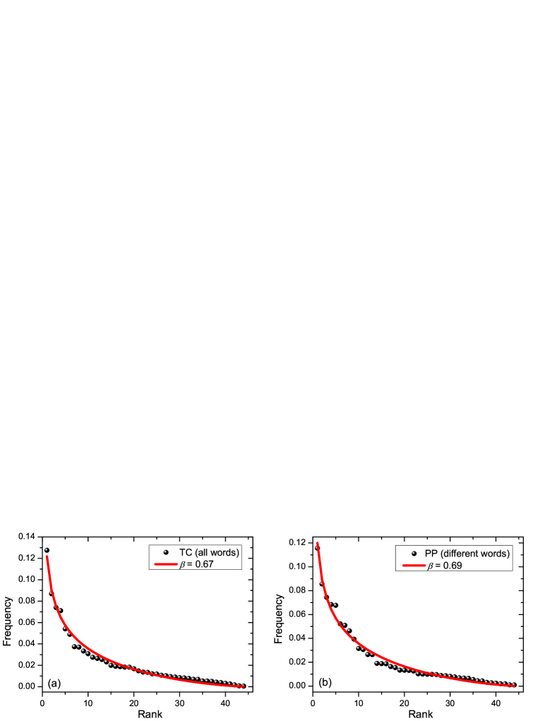
Figure 2: Rank-frequency relation (black circles) and the fitting with Dirichlet distribution (red line). (a) Left figure: text TC, where frequencies were extracted from all words. (b) Right figure: text PP, where different words were employed; see Table I for the description of texts.

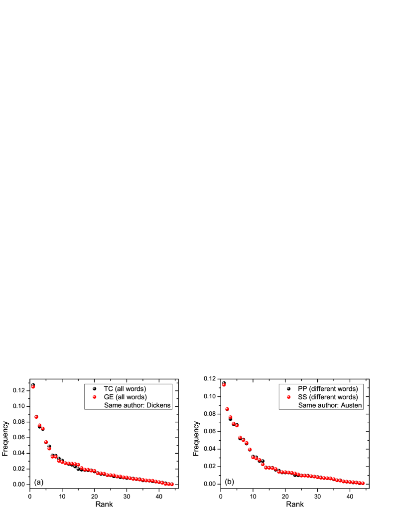
Figure 3: Rank-frequency relation (black and red circles) for two texts written by the same author. (a) Left figure: TC and GE written by Dickens (all words were employed for extracting the phoneme frequencies). (b) Right figure: PP and SS written by Austen (different words were employed); see Table I.

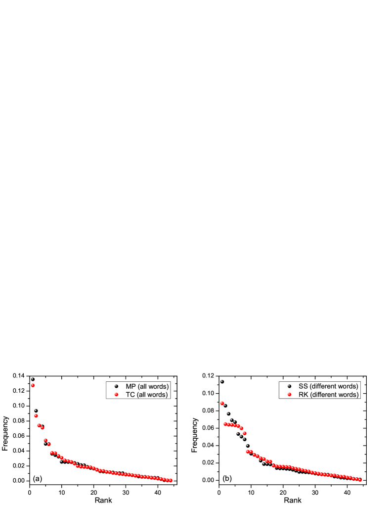
Figure 4: Rank-frequency relation (black and red circles) for two texts written by different authors. (a) Left figure: TC by Dickens versus MP by Austen (all words were employed). (b) Right figure: SS by Austen versus RK by Tolkien (different words were employed); see Table I for parameters of these texts.

In the next section we shall see that the sequence of ordered probabilities $f_{r}$ [cf. (1)] can be generated via (7). To this end, the empiric quantities $f_{r}$ will be compared to $\hat{f}_{r}=\langle\theta_{(r)}\rangle$; cf. (9). The rationale for using the average is that for parameters we are interested in|where $n\simeq 40-50$ (for English phonemes $n=44$) and $0.5\leq\beta\leq 1$|we get from (7–9) that relative fluctuations around the average $\hat{f}_{r}\equiv\langle\theta_{(r)}\rangle$ are small. Namely, $\varepsilon_{r}\equiv(\langle\theta_{(r)}^{2}\rangle-\langle\theta_{(r)}\rangle^{2})/\langle\theta_{(r)}\rangle^{2}\lesssim 0.02$ for all values of $r$, excluding $r\approx n$, i.e. very low frequency phonemes. This is shown in Fig. 1 for a particular value $\beta=0.8$. Note that $\varepsilon_{r}$ is not a monotonic function of $r$: it is smallest for middle ranks. (Even for those values of $r$, where $\varepsilon_{r}\simeq 1$, $\hat{f}_{r}=\langle\theta_{(r)}\rangle$ can still describe the empiric frequencies $f_{r}$, as seen below.) Now there is a simpler approximate formula for $\hat{f}_{r}=\langle\theta_{(r)}\rangle$ that is deduced from (9) [see section II of the supplementary material]:

$$\frac{r}{n}=1-\varphi(\hat{f}_{r}n\beta).$$ (10)

Fig. 1 shows that $\hat{f}_{r}$ obtained from (10) indeed approximates well $\langle\theta_{(r)}\rangle$ for almost all ranks $r$.

III Results

III.1 Fitting rank-frequency relations to the Dirichlet distribution

Table 1: Nine texts and their parameters. Texts are abbreviated and numbered. $N_{tw}$, $N_{pht}$, $N_{dw}$ and $N_{phd}$ are, respectively, the total number of words, the number of phonemes of the total words, the number of different words and the number of phonemes of different words.
J. Austen: Mansfield Park (MP or 1) 1814; Pride and Prejudice (PP or 2) 1813; Sense and Sensibility (SS or 3) 1811.
C. Dickens: A Tail of Two Cities (TC or 4) 1859; Great Expectations (GE or 5) 1861; Adventures of Oliver Twist (OT or 6) 1838.
J. Tolkien: The Fellowship of the Ring (FR or 7) 1954; The Return of the King (RK or 8) 1955; The Two Towers (TT or 9) 1954.

Texts	$N_{tw}$	$N_{pht}$	$N_{dw}$	$N_{phd}$
MP (1)	160473	567750	7854	48747
PP (2)	121763	435322	6385	39767
SS (3)	119394	425822	6264	38668
TC (4)	135420	468642	9841	58760
GE (5)	186683	623079	10933	65364
OT (6)	159103	555372	10359	61072
FR (7)	177227	617106	8644	46509
TT (8)	143436	502303	7676	39823
RK (9)	134462	431141	7087	36494

Table 2: Fitting parameters for texts numbered as 1-9; see (11, 12) and Table I for text numbers. The phoneme frequencies are extracted from all words of the text; see Table III for the values of $\beta$ calculated from different words of texts.

	1	2	3	4	5	6	7	8	9
$\beta$	0.61	0.63	0.61	0.67	0.69	0.69	0.75	0.74	0.79
$SS_{err}\times 10^{7}$	7696	7574	6151	4317	5287	3993	4196	4337	3580
$R^{2}$	0.9768	0.9765	0.9816	0.9859	0.9820	0.9867	0.9844	0.9842	0.9860

Table 3: Fitting parameters for texts numbered as 1-9; see (11, 12) and Table I for text numbers. The phoneme frequencies are extracted from different words of the text; see Table II for the values of $\beta$ calculated from all words of texts. Eqs. (17, 18) compare the data presented in Tables II and III.

	1	2	3	4	5	6	7	8	9
$\beta$	0.72	0.69	0.69	0.77	0.78	0.79	0.968	0.979	0.975
$SS_{err}\times 10^{7}$	5150	4495	5003	6107	5265	5220	11296	12943	10366
$R^{2}$	0.9818	0.9847	0.9829	0.9771	0.9800	0.9800	0.9501	0.9403	0.9525

We studied 48 English texts written by 16 different, native-English authors; see Table I and section III of the supplementary material. For each text we extracted the phoneme frequencies $\{f_{r}\}_{r=1}^{n}$ and ordered them as in (1); the list of English phonemes is given in section I of the supplementary material. The transcription of words into phonemes was carried out via the software PhoTransEdit, which is available at pho . This is a relatively slow, but very robust software, since it works by checking each word in the phonetic dictionary. Thus it can err only on those unlikely cases, when the word is not found in the dictionary.

It is important to specify from which set of words (of a text) one extracts the phoneme frequencies. Two natural choices are possible here: either one employs all words of the text, or different words of the text (i.e. multiple occurrences of the same word are neglected). We shall study both cases. For clarity reasons, we shall present our results by focussing on the three authors mentioned in Table I. Three texts by three authors is in a sense the minimal set-up for described effects. We stress that other texts we studied fully corroborate our results; they are partially described in Table 4 below and in section III of the supplementary material.

The ordered set $\{f_{r}\}_{r=1}^{n}$ of phoneme frequencies for each text was compared with the prediction $\{\hat{f}_{r}=\langle\theta_{(r)}\rangle\}_{r=1}^{n}$ of the Dirichlet density [see (9)]. Here the parameter $\beta$ [cf. (2, 5)] is found from minimizing the error:

$$SS_{err}=\sum_{k=1}^{n}(f_{k}-\hat{f}_{k})^{2}.$$ (11)

For each studied case we also monitored the coefficient of correlation between $\{f_{r}\}_{r=1}^{n}$ and $\{\hat{f}_{r}\}_{r=1}^{n}$:

$$R^{2}=\frac{\left[\,\sum_{k=1}^{n}(f_{k}-\bar{f})(\hat{f}_{k}-\overline{\hat{f}})\,\right]^{2}}{\sum_{k=1}^{n}(f_{k}-\bar{f})^{2}\sum_{k=1}^{n}(\hat{f}_{k}-\overline{\hat{f}})^{2}},$$ (12)

where

$$\bar{f}\equiv\frac{1}{n}{\sum}_{k=1}^{n}f_{k},\qquad\overline{\hat{f}}\equiv\frac{1}{n}{\sum}_{k=1}^{n}\hat{f}_{k}.$$ (13)

A good fitting means that $R^{2}$ is close to $1$. We found that (as functions of $\beta$) $SS_{err}$ and $1-R^{2}$ minimize simultaneously.

Examples of fitting curves for phoneme rank-frequency relations are presented in Fig. 2. The fitting parameters are given in Tables II and III. Note that the fitting values of $R^{2}$ are good. The group of most frequent eight phonemes reads [see section I of the supplementary material]: /ı/,  //,  /n/,  /s/,  /t/,  /l/,  /d/,  /r/. The concrete ranking between them depends on the text, but the most frequent one is normally /ı/.

Tables II and III show that the texts by the same author have closer values of $\beta$ than those written by different authors; see also Figs. 3 and 4. This can be quantified via the following three inequalities

$$0<b({\rm A})\equiv{\rm min\,}\{|\beta_{i}-\beta_{k}|\}_{i=1,2,3;k=4,5,6,7,8,9}\,-\,{\rm max\,}\{|\beta_{i}-\beta_{j}|\}_{i<j;i,j=1,2,3},$$ (14)

$$0<b({\rm D})\equiv{\rm min\,}\{|\beta_{i}-\beta_{k}|\}_{i=4,5,6;k=1,2,3,7,8,9}\,-\,{\rm max\,}\{|\beta_{i}-\beta_{j}|\}_{i<j;i,j=4,5,6},$$ (15)

$$0<b({\rm T})\equiv{\rm min\,}\{|\beta_{i}-\beta_{k}|\}_{i=7,8,9;k=1,2,3,4,5,6}\,-\,{\rm max\,}\{|\beta_{i}-\beta_{j}|\}_{i<j;i,j=7,8,9},$$ (16)

where A, D and T refer, respectively to Austen, Dickens and Tolkien [see Table I]. The indices $i$ and $j$ run over the texts by the same author, while $k$ refer to different authors, e.g. $i,j=\{1,2,3\}$ (Austen) and $k=\{4,5,6,7,8,9\}$ (not Austen). The minimization (or maximization) in (14-16) goes over indicated indices.

Eqs. (14-16) hold both for phoneme frequencies extracted from different words and from all words of a text; cf. Tables II and III. For instance, $b^{\rm[all~{}words]}({\rm A})=0.02$, $b^{\rm[all~{}words]}({\rm D})=0.02$, $b^{\rm[all~{}words]}({\rm T})=0$. The latter is the only minor exclusion from (14-16).

Thus the set $\{\beta_{i}\}_{i=1}^{9}$ fragments into three clusters that refer to different authors. Note that

$$b^{\rm[diff.~{}words]}(a)>b^{\rm[all~{}words]}(a),\qquad a={\rm A,\,D,\,T}.$$ (17)

Hence different words display the author-dependency in a stronger form; this is confirmed below by other methods.

The author-dependency of phoneme rank-frequency relation is unexpected, because the rank-frequency relation for words (which consists of phonemes) follows the Zipf's law whose shape is independent of the author wyllis ; baa ; zipf_pre . Note that the few most frequent phonemes and the least frequent ones appear to fit best the theoretical prediction; cf. Fig. 2. This feature again contrasts the rank-frequency relation for words, where it is known that high-frequency words|these are mostly the functional words, e.g. and, or|do hold the Zipf's law worst than other words zipf_pre . On the other hand, the moderate-frequency phonemes deviate most from the prediction of the Dirichlet curve; cf. Fig. 2. This effect is not statistical, since fluctuations around the average are most suppressed for moderate-frequency phonemes; see after (9) and Figs. 1 and 2.

Another pertinent result is that [see Tables II and III]

$$\beta_{i}^{\rm[diff.~{}words]}>\beta_{i}^{\rm[all~{}words]},~{}\qquad i=1,...,9,$$ (18)

i.e. the phoneme distribution obtained from different words is more homogeneous [see our discussion after (5)], because for all words the frequency of high-rank phonemes is amplified due to multiple usage of frequent words.

Note that the above three texts belong to one genre (novels) and concern only three authors. Hence we studied other 13 native-English authors who created in XIX'th and the first half of XX'th century; see section III of the supplementary material. These additional studies corroborate the obtained results. In particular, Table 4 presents the values of $\beta$ extracted from different texts of 5 authors. These authors were selected so that their language differences due to social, temporal and professional backgrounds are minimized. In addition, we selected 4 of them to be professional scientists, since the language of scientific works is normally more unified. Lyell, Darwin, Wallace, and Spenser were naturalists, while the fifth author (H.G. Wells) held a PhD in biology and wrote a lot about scientists. Lyell strongly influenced Darwin, while Darwin and Wallace were close colleagues. All these three naturalists influenced Spenser and Wells. However, Table 4 shows that the values of $\beta$ for these 5 authors are clearly different and hold analogues of (14-16).

We want to stress that $\beta$ anyhow changes in a bounded interval: $0.5<\beta<1$. Hence if one takes sufficiently many authors, their values of $\beta$ will start to overlap. In our study of (overall) 16 authors we confirmed this expectation; see section III of the supplementary material. However, these overlaps are accidental, i.e. the overlapping authors can be easily distinguished by alternative means. In particular, their phoneme distributions can be robustly distinguished via distances, as described below.

Table 4: The values of $\beta$ extracted from different words of texts for 5 authors. For each author we analyzed three texts. They are described in the supplementary material, where we also discuss 8 other authors.

C. Lyell	0.798	0.785	0.792
A. R. Wallace	0.744	0.756	0.739
C. Darwin	0.817	0.810	0.822
H. Spenser	0.646	0.658	0.650
H. G. Wells	0.737	0.735	0.724

III.2 Distance between phoneme frequencies

The author-dependency of phoneme rank-frequency relation is corroborated by looking directly at suitable distances between the ranked phoneme frequencies in different texts. We choose to work with the variational distance

$$\rho_{1}(ij)=\frac{1}{2}\sum_{k=1}^{n}|\,f_{k}[i]-f_{k}[j]\,|,$$ (19)

where $\{f_{k}[i]\}_{k=1}^{n}$ are the ordered phoneme frequencies in the text $i$. We shall also employ a more fine-grained (detail-specific) distance. Let $f[\alpha|i]$ be the frequency of phoneme $\alpha$ in text $i$ ($\alpha=1,...,n$, $i=1,..,9$). We can now define [cf. (19)]

$$\rho_{0}(ij)=\frac{1}{2}\sum_{\alpha=1}^{n}|\,f[\alpha|i]-f[\alpha|j]\,|.$$ (20)

Now $\rho_{0}(ij)=0$ only if $f[\alpha|i]=f[\alpha|j]$. It is seen from Tables V-VII that $\rho_{0}(ij)>\rho_{1}(ij)$, as it should be, because $\rho_{1}(ij)$ is less sensitive to details (i.e. it is more coarse-grained).

To motivate the choice of the variational distance $\rho_{0}=\frac{1}{2}\sum_{\alpha=1}^{n}|\,p_{\alpha}-q_{\alpha}\,|$ between two sets of probabilities $\{p_{\alpha}\}_{\alpha=1}^{n}$ and $\{q_{\alpha}\}_{\alpha=1}^{n}$, let us recall an important feature of this distance gibbs : $\rho_{0}={\rm max}_{\Omega}\left|\sum_{\alpha\in\Omega}(p_{\alpha}-q_{\alpha})\,\right|$, where the maximization goes over all sub-sets $\Omega$ of $\{1,...,n\}$. Thus $\rho_{0}$ refers to the (composite) event that gives the largest probability difference between $\{p_{\alpha}\}_{\alpha=1}^{n}$ and $\{q_{\alpha}\}_{\alpha=1}^{n}$.

Tables V and VI refer, respectively, to phoneme frequencies extracted from all words and different words of the text. These tables show that phoneme rank-frequency relations between the texts written by the same author are closer to each other|in the sense of distances $\rho_{0}$ and $\rho_{1}$|than the ones written by different authors. This is also seen on Figs. 3 and 4.

To quantify these differences, consider the following inequalities that define clustering with respect to authors (see Table I for numbering of texts, and note that $\rho_{\lambda}(ij)=\rho_{\lambda}(ji)$ for the distance between the texts $i$ and $j$):

$$0<z_{\lambda}({\rm A})\equiv{\rm min\,}\{\rho_{\lambda}(ik)\}_{i=1,2,3;k=4,5,6,7,8,9}\,-\,{\rm max\,}\{\rho_{\lambda}(ij)\}_{i<j;i,j=1,2,3},~{}~{}\lambda=0,1,$$ (21)

$$0<z_{\lambda}({\rm D})\equiv{\rm min\,}\{\rho_{\lambda}(ik)\}_{i=4,5,6;k=1,2,3,7,8,9}\,-\,{\rm max\,}\{\rho_{\lambda}(ij)\}_{i<j;i,j=4,5,6},~{}~{}\lambda=0,1,$$ (22)

$$0<z_{\lambda}({\rm T})\equiv{\rm min\,}\{\rho_{\lambda}(ik)\}_{i=7,8,9;k=1,2,3,4,5,6}\,-\,{\rm max\,}\{\rho_{\lambda}(ij)\}_{i<j;i,j=7,8,9},~{}~{}\lambda=0,1,$$ (23)

where A, D and T refer, respectively to Austen, Dickens and Tolkien; cf. (21–23) with (14-16). For example, the maximal distance (20) between texts by Austen (see Table I) is denoted by ${\rm max\,}\{\rho_{0}(ij)\}_{i<j;i,j=1,2,3}$, while ${\rm min\,}\{\rho_{0}(kl)\}_{k=1,2,3;l=4,5,6,7,8,9}$ is the minimal distance between texts written by Austen and those written by Dickens and Tolkien. Note that (21–23) hold as well for other 13 authors we analyzed; see section III of the supplementary material for examples.

The meaning of (21–23) can be clarified by looking at an authorship attribution task: let several texts $i=1,2,3$ by (for example) Austen are at hands, and one is given an unknown text $\alpha$. The question is whether $\alpha$ could also be written by Austen. If now ${\rm max}_{i}[\rho_{\lambda}(i\alpha)]\leq{\rm max}_{i<j}[\rho_{\lambda}(ij)]$, we have an evidence that $\alpha$ is written by Austen.

We stress that there are no fitting parameters in (20–23). Our data (cf. Tables V and VI) holds eleven (out of twelve) inequalities (21–23) for phoneme frequencies extracted both from different and from all words of the text. There is only one exclusion: $z_{1}^{\rm[all~{}words]}({\rm T})=-0.00207$, which is by an order of magnitude smaller than the respective frequencies [cf. (23)]. Apart of this minor exclusion, we confirm the above prediction (obtained via the fitted values of $\beta$) on the author-dependency for phoneme frequencies.

Data shown in Tables V (all words) and VI (different words) also imply the following inequalities [confirming (17)]

$$z_{\lambda}^{\rm[diff.~{}words]}(a)>z_{\lambda}^{\rm[all~{}words]}(a),\qquad\lambda=0,1,\qquad a={\rm A,\,D,\,T}.$$ (24)

Another pertinent feature is that the distances $\rho_{0}$ and $\rho_{1}$ between texts written by the same author hold

$$\rho^{\rm[all~{}words]}_{\lambda}(ij)>\rho^{\rm[diff.~{}words]}_{\lambda}(ij),$$ (25)

$$\lambda=0,1,\quad(ij)=\{\,(12),(13),(23),(45),(46),(78),(79),(89)\,\}.$$

Seventeen out of eighteen relations (25) hold for our data; see Tables V and VI, where we present the distances $\rho_{0}$ and $\rho_{1}$ for phoneme frequencies deduced from, respectively, all words and different words of the texts. The only exclusion in (25) is $\rho^{\rm[diff.~{}words]}_{0}(78)-\rho^{\rm[all~{}words]}_{0}(78)=0.02853-0.02584=0.00269$. No definite relations exist between $\rho^{\rm[all~{}words]}_{\lambda}$ and $\rho^{\rm[diff.~{}words]}_{\lambda}$ for texts written by different authors. One can interpret (25) as follows. When going from different words to all words of the text, the majority of frequent words are not author-specific: they are mostly key-words (that are specific to the text, but not necessarily to the author) and functional words (e.g. and, or, of, but) that are again not author-specific.

Taken together, (24) and (25) imply that the clustering with respect to authors is better visible for frequencies extracted from different words of the texts (the inter-cluster distance increases, whereas the intra-cluster distance decreases). The same effect was obtained above via fitted values of $\beta$'s; see (17).

Table 5: Distances $\rho_{0}$ and $\rho_{1}$ between texts; see Table I and (20–19) for the definition of $\rho_{0}$ and $\rho_{1}$. The phoneme frequencies are extracted from all words of the text. Eqs. (24, 25) compare the distances from all words with those from different words.

	12	13	23	45	46	56	78	79	89
$\rho_{0}\times 10^{5}$	3045	2062	2549	3423	2382	3448	2584	2066	2464
$\rho_{1}\times 10^{5}$	2227	1602	2103	2100	1978	2753	1808	1809	2037

	14	15	16	17	18	19	24	25	26	27	28	29
$\rho_{0}\times 10^{5}$	3583	4690	4000	7372	7402	7322	3645	4762	4064	7653	7629	7650
$\rho_{1}\times 10^{5}$	2784	3044	3260	5149	5227	5599	2712	3059	3110	4978	5052	5449

	34	35	36	37	38	39	47	48	49	57	58	59	67	68	69
$\rho_{0}\times 10^{5}$	3562	4924	4358	7737	6950	7447	5174	5327	5061	6113	6436	6217	5074	5706	5202
$\rho_{1}\times 10^{5}$	2546	3022	3181	5266	5085	5654	3950	3568	3935	3894	4014	4325	3727	3934	3770

Table 6: Distances $\rho_{0}$ and $\rho_{1}$ between texts; see Table I and (20–19). The phoneme frequencies are extracted from different words of the text; see (24, 25) for comparison with all words.

	12	13	23	45	46	56	78	79	89
$\rho_{0}\times 10^{5}$	1563	1317	1413	1568	1380	1100	2853	1946	2025
$\rho_{1}\times 10^{5}$	1346	1205	1346	1266	1126	1052	1635	1476	1569

	14	15	16	17	18	19	24	25	26	27	28	29
$\rho_{0}\times 10^{5}$	2296	2703	2868	7430	9535	8434	2839	3318	3458	8141	9999	9167
$\rho_{1}\times 10^{5}$	1967	2110	2470	6103	7200	6775	2252	2436	2709	6587	7544	7136

	34	35	36	37	38	39	47	48	49	57	58	59	67	68	69
$\rho_{0}\times 10^{5}$	2718	3264	3257	7943	9998	8997	5918	7875	6899	5521	7842	6646	5595	7785	6786
$\rho_{1}\times 10^{5}$	2193	2486	2636	6539	7447	7022	4795	5971	5368	4631	5566	5222	4486	5645	5201

Table 7: Distances $\rho_{0}$ and $\rho_{1}$ between texts; see Table I and (20–19). The phoneme frequencies are extracted from different words of each text after excluding the words that are common for both compared texts; see (26, 27) for comparison with the situation without excluding common words.

	12	13	23	45	46	56	78	79	89
$\rho_{0}\times 10^{5}$	3792	3217	3734	3146	2930	2329	5918	4421	4770
$\rho_{1}\times 10^{5}$	2832	2463	2502	2190	2215	1610	3317	2773	2809

	14	15	16	17	18	19	24	25	26	27	28	29
$\rho_{0}\times 10^{5}$	4758	5742	6087	12574	15119	13490	5708	6385	6880	13323	15733	14113
$\rho_{1}\times 10^{5}$	3912	4276	4830	8800	9576	8895	4529	4991	5495	9469	10387	9621

	34	35	36	37	38	39	47	48	49	57	58	59	67	68	69
$\rho_{0}\times 10^{5}$	5188	5887	6476	13391	15842	14244	10980	13905	12109	10346	13003	11673	10413	13288	11911
$\rho_{1}\times 10^{5}$	4344	4917	5285	9835	10637	9891	7025	7371	6928	6537	7021	6673	6580	6667	6433

Table 8: The fraction $p$ of common words between texts given in Table I. Now $p$ is defined as follows. Let $n(i)$ and $n(ij)$ be, respectively, the number of different words in text $i$ and the number of common words in texts $i$ and $j$. We define: $p(ij)=n(ij)/(n(i)+n(j)-n(ij))$, where $0\leq p(ij)\leq 1$. This is the number of common words divided over the number of all different words in texts $i$ and $j$. As seen from the data below, analogues of (21–23) hold with $1-p(ij)$ instead of $\rho_{\lambda}(ij)$.

	12	13	23	45	46	56	78	79	89
$p\times 10^{5}$	47554	47786	50655	41146	42454	41822	45010	46948	48173

	14	15	16	17	18	19	24	25	26	27	28	29
$p\times 10^{5}$	35592	35819	36660	28978	25870	26730	32902	32499	33877	26549	24180	24643

	34	35	36	37	38	39	47	48	49	57	58	59	67	68	69
$p\times 10^{5}$	33463	32813	34643	27572	25340	25733	33901	30387	32005	32069	27963	29994	32002	28649	30518

III.3 The origin of the author-dependency effect is not in common words

One possible reason for the author-dependency of phoneme frequencies is that the effect is due to the vocabulary of the author. In this scenario the similarity between phoneme frequencies in text written by the same author would be caused by the fact that these texts have sufficiently many common words that carry out the same phonemes.

Texts written by the same author do have a sizeable number of common words, as was already noted within the authorship attribution research joula ; ule . We confirm this result in Table VIII, where it is seen that the fraction of common words holds the analogues of (21–23). Hence this fraction also shows the author-dependency effect.

In order to understand whether the author-dependency of phoneme frequencies can be explained via common words, we excluded from different words of texts $i$ and $k$ the common words of those texts [$i,k=1,...,9$, see Table I], re-calculated phoneme frequencies, and only then determined the respective distances $\rho_{0}^{\rm[no~{}comm.~{}words]}(ik)$ and $\rho_{1}^{\rm[no~{}comm.~{}words]}(ik)$. If the explanation via common words holds, they will not show author-dependency. This is however not the case: the effect is there because relations (21–23) do hold for them

$$z_{\lambda}^{\rm[no~{}comm.~{}words]}(a)>0,\qquad\lambda=0,1,\qquad a={\rm A,\,D,\,T}.$$ (26)

Eq. (26) is deduced from Table VII, where we present the distances $\rho_{0}$ and $\rho_{1}$ for the situation, where the common words are excluded.

After excluding the common words the author-dependency did not get stronger in the sense of (25), because the data of Tables VI (different words) and VII (excluded common words) imply for texts written by the same author

$$\rho^{\rm[no~{}comm.~{}words]}_{\lambda}(ij)>\rho^{\rm[diff.~{}words]}_{\lambda}(ij),\qquad\lambda=0,1,$$ (27)

$$\quad(ij)=\{\,(12),(13),(23),(45),(46),(78),(79),(89)\,\}.$$

In this context recall (24, 25). But it also did not get weaker [cf. (24) and (21–23)], because

$$z_{\lambda}^{\rm[no~{}comm.~{}words]}(a)>z_{\lambda}^{\rm[diff.~{}words]}(a),\qquad\lambda=0,1,\qquad a={\rm A,\,D,\,T},$$ (28)

as seen from Tables VI and VII, which refer, respectively, to different words and the excluded common words.

IV Summary

Phonemes are the minimal building blocks of the linguistic hierarchy that still relate to meaning. A coarse-grained description of phoneme frequencies is provided by rank-frequency relations. For describing these relations we followed the qualitative analogy between atoms and phonemes zwick ; abler . Atoms amount to a finite (and not very large) number of discrete elements from which the multitude of substances and materials are built balian . Likewise, a finite number of phonemes can construct a huge number of texts abler .

The simplest description of an (sufficiently dilute) atomic system is provided via the ideal gas model balian . By studying 16 native-English authors, we show that the rank-frequency relations for phonemes can be described via the ordered statistics of the Dirichlet density, the direct analogue of the ideal gas model in statistics. In particular, though the number of phonemes is not very large (English has 44 phonemes), it is just large enough to validate the statistical description. The single parameter of the Dirichlet density corresponds to the (inverse) temperature of the ideal gas in statistical physics. It appears that the most frequent phonemes fit the Dirichlet distribution much better than others. This contrasts to the rank-frequency relations for words, where the Zipf's law holds worst for the most frequent words.

The fitting to the Dirichlet density uncovers an important aspect of phoneme frequencies: they depend on the author of the text. This fact is seen for authors who created their works in various genres (novels, scientific texts, journal papers), and also for authors whose language-dependence on social, temporal and educational background has been minimized (e.g. the closely inter-related group of English naturalists including Darwin, Wallace, Lyell, and Spencer). We confirmed this result via a parameter-free method that is based on calculating distances between phoneme frequencies of different texts. Again, this contrasts to the Zipf's law for rank-frequency relations of words whose shape is author-independent.

It is well-known that certain aspects of text-statistics display author-dependency, and this is applied in various author attribution tasks; see e.g. gibbs ; ule ; joula ; koppel ; stama ; kuku for recent reviews. In particular, this concerns frequencies of functional words. The fact that author-dependency is seen on such a coarse-grained level as rank-frequency relations may mean that phoneme frequencies can be useful for existing methods of authorship attribution joula ; koppel ; stama ; kuku . This should be clarified in future.

A straightforward reason for explaining the author-dependency effect of phoneme frequencies would be that it is due to the author's vocabulary, as reflected by common words in texts written by the same author. The previous section has shown that such an explanation is ruled out.

Then we are left with options that the effect is due to storing (with different frequencies) syllables or/and phonemes. If syllable frequencies have author-dependency, this could result to author-dependent phoneme frequencies, because there are specific rules that (at least probabilistically) determine the phoneme composition of syllables kessler . But note that syllables are in several respect similar to words (and not phonemes): (i) there are many of them; e.g. English has more than 12000 syllables. (ii) There is large gap between frequent and infrequent syllables levelt (cf. with the hapax legomena for words). (iii) There are indications that syllables are stored in a syllabic lexicon that in several ways is similar to the mental lexicon that stores words levelt .

The second possibility would mean that the authors store phonemes nathan , and this will provide a statistical argument for psychological reality of phonemes. Note that the issue of psychological reality of a phoneme is not settled in modern phonology and psychology, various schools arguing pro and contra of it; see port ; suomi ; nathan ; savin ; foss for discussions. And then both these options might be present together. Thus further research|also involving rank-frequency relations for syllables|is needed for clarifying the situation.

The presented methods can find applications in animal communication systems. In this context, we recall an interesting argument ivanov . The number of phonemes in languages roughly varies between $20$ and $50$. Indeed, the average number of phonemes in European languages is $\simeq 37$. (English has 44 phonemes, but if diphthongs are regarded as combinations of a vowel and a semi-vowel this number reduces to 36.) In tonal languages the overall number of phonemes is larger, e.g. it is $\sim 180$ for Chinese. (The tone produces phonemes and not allophones, since they do change the meaning.) But the number of phonemes without tones still complies with the above rough bound. Since Old Chinese (spoken in 11 to 7'th centuries B.C.) lacked tones, the tonal phonemes of modern Chinese evolved from their non-tonal analogues that complies with the above number sampson . By its order of magnitude this number ($\sim 20-50$) coincides ivanov with the number of ritualized (i.e. sufficiently abstract) signals of animal communication, which is also stable across different species moynihan . (An example of this are gestures of apes.) This number is sufficiently large to invite the application of the presented statistical methods to signals of animal communication. And the stability of this number may mean that there are further similarities (to be yet uncovered) between phonemes and ritualized signals.

Supplementary material

I. English phonemes

Here we recall $44$ English phonemes according to the International Phonetic Alphabet.

I. $20$ vowels (7 short phonemes, 5 long and 8 diphtongs):

(but), æ  (cat),   (about), e (men), ı  (sit),   (not),   (book),

: (part), : (word, learn), i: (read), : (sort), u: (too),

aı  (my), a  (how), o  (go), eı  (day), ı  (here), oı  (boy),   (tour, pure), e  (wear, fair)

II. $24$ consonants:

b   (born), d   (do), f   (five), g   (get), h   (house), j   (yes), k   (cat), l   (lion), m   (mouse), n   (nouse),   (sing), p   (put), r   (room), s   (saw),   (shall), t   (time),   (church),   (think), $\eth$   (the), v   (very), w   (window), z   (zoo),   (casual), d  (judge)

II. Order statistics for Dirichlet density

Let us introduce the following notation for the order integration

$${\cal I}({\rm d}\theta_{1},...,{\rm d}\theta_{n})\equiv\int_{0}^{\infty}{\rm d}\theta_{1}\int_{0}^{\theta_{1}}{\rm d}\theta_{2}...\int_{0}^{\theta_{n-1}}{\rm d}\theta_{n}.$$ (29)

Now the average over the order statistics of the Dirichlet density is defined as

$$\langle\theta_{(r)}^{m}\rangle=\frac{{\cal I}({\rm d}\theta_{1},...,{\rm d}\theta_{n})\,\theta_{r}^{m}\,\delta(\sum_{k=1}^{n}\theta_{k}-1)\,\prod_{k=1}^{n}\theta_{k}^{\beta-1}}{{\cal I}({\rm d}\theta_{1},...,{\rm d}\theta_{n})\,\delta(\sum_{k=1}^{n}\theta_{k}-1)\,\prod_{k=1}^{n}\theta_{k}^{\beta-1}}.$$ (30)

In the numerator of (30) we change variables as $\hat{\theta}_{k}=r\theta_{k}$ ($r>0$), multiply both sides by $e^{-r}$, and then integrate both sides over $r\in[0,\infty)$:

$${\cal I}({\rm d}\theta_{1},...,{\rm d}\theta_{n})\,\theta_{r}^{m}\,\delta(\sum_{k=1}^{n}\theta_{k}-1)\,\prod_{k=1}^{n}\theta_{k}^{\beta-1}\times\Gamma[n\beta+m]={\cal I}({\rm d}\hat{\theta}_{1},...,{\rm d}\hat{\theta}_{n})\,\hat{\theta}_{r}^{m}\prod_{k=1}^{n}\hat{\theta}_{k}^{\beta-1}e^{-\hat{\theta}_{k}}.$$ (31)

The denominator of (30) is worked out analogously.

Let us now define

$$\chi_{r}(y;m)=\frac{\Gamma[n\beta]}{\Gamma[n\beta+m]}\,\frac{{\cal I}({\rm d}\hat{\theta}_{1},...,{\rm d}\hat{\theta}_{n})\,\delta(y-\hat{\theta}_{r})\,\prod_{k=1}^{n}\hat{\theta}_{k}^{\beta-1}e^{-\hat{\theta}_{k}}}{{\cal I}({\rm d}\hat{\theta}_{1},...,{\rm d}\hat{\theta}_{n})\,\prod_{k=1}^{n}\hat{\theta}_{k}^{\beta-1}e^{-\hat{\theta}_{k}}}$$ (32)

so that the following relation holds

$$\langle\theta_{(r)}^{m}\rangle=\int_{0}^{\infty}{\rm d}y\,y^{m}\chi_{r}(y;m).$$ (33)

This is the equation (9) of the main text. Working out ${\cal I}({\rm d}\hat{\theta}_{1},...,{\rm d}\hat{\theta}_{n})\,\prod_{k=1}^{n}\hat{\theta}_{k}^{\beta-1}e^{-\hat{\theta}_{k}}$ and ${\cal I}({\rm d}\hat{\theta}_{1},...,{\rm d}\hat{\theta}_{n})\,\delta(y-\hat{\theta}_{r})\,\prod_{k=1}^{n}\hat{\theta}_{k}^{\beta-1}e^{-\hat{\theta}_{k}}$ in (32) via integration by parts (starting from the last integration in ${\cal I}({\rm d}\hat{\theta}_{1},...,{\rm d}\hat{\theta}_{n})$) we obtain equations (7–9) of the main text.

If $(n-r)\gg 1$ and $r\gg 1$ the behavior of $\chi_{r}(y;m)$ in equations (7) of the main text is determined by the exponential factor $e^{(n-r)\ln\varphi(y)+r\ln(1-\varphi(y))}$. Working it out via the saddle-point method we conclude that asymptotically:

$$\chi_{r}(y;m)\simeq\frac{\Gamma[n\beta]}{\Gamma[n\beta+m]}\,\frac{1}{\sqrt{2\pi\sigma}}\,e^{-\frac{1}{2\sigma}(y-y_{0})^{2}},$$ (34)

where $y_{0}$ and $\sigma$ are defined as follows

$$\frac{n-r}{n}=\varphi(y_{0}),~{}~{}~{}~{}\sigma=\frac{(n-r)r}{n^{3}}\,\frac{1}{[\,\varphi^{\prime}(y_{0})\,]^{2}},$$ (35)

where $\phi^{\prime}(y)={\rm d}\varphi(y)/{\rm d}y$.

Hence we get from (33) and (34, 35):

$$\langle\theta_{(r)}\rangle=\frac{y_{0}}{n\beta},$$ (37)

$$\langle\theta_{(r)}^{2}\rangle-\langle\theta_{(r)}\rangle^{2}=\frac{n\beta\sigma-y_{0}^{2}}{[n\beta]^{2}(n\beta+1)}=\frac{1}{[n\beta]^{2}(n\beta+1)}\left(\frac{\beta(n-r)r}{n^{2}}\,\frac{1}{[\varphi^{\prime}(y_{0})]^{2}}-y_{0}^{2}\right).$$

The importance of fluctuations is characterized by

$$\frac{\langle\theta_{(r)}^{2}\rangle-\langle\theta_{(r)}\rangle^{2}}{\langle\theta_{(r)}\rangle^{2}} = \frac{1}{n\beta+1}\left(\frac{\beta(n-r)r}{n^{2}}\,\frac{1}{y_{0}^{2}[\varphi^{\prime}(y_{0})]^{2}}-1\right)$$ (38)

$$= \frac{1}{n\beta+1}\left(\frac{\beta(n-r)r}{n^{2}}\,\,\Gamma^{2}[\beta]\,y_{0}^{-2\beta}\,e^{2y_{0}}-1\right),$$ (39)

where we employed

$$\varphi(y)=\frac{1}{\Gamma[\beta]}\int_{0}^{y}{\rm d}x\,x^{\beta-1}e^{-x}$$ (40)

This is the equation (8) of the main text. Eq. (39) is a good approximation of $\frac{\langle\theta_{(r)}^{2}\rangle-\langle\theta_{(r)}\rangle^{2}}{\langle\theta_{(r)}\rangle^{2}}$ calculated (exactly) from equations (7-9) of the main text; see Fig. 1 of the main text.

III. Information on the other 13 authors and 39 texts

Here are the works by the other 13 English writers we studied in addition to the authors described in Table I of the main text. After the title of each work we give its writing/publication date, the number of different words, and the number of phonemes of different words. The table below summarizes the values of $\beta$ for phonemes extracted from different words of each text.

Charlotte Bronte: Jane Eyre (1847, 12488, 75933), Shirley (1849, 14481, 88911), Villette (1853, 14176, 88025).

Clive S. Lewis: Perelandra (1943, 7030, 41265), Out of the Silent Planet (1938, 6045, 35371), That Hideous Strength (1946, 7842, 46618).

George Eliot: Adam Bede (1859, 9685, 56819), Romola (1862, 13402, 83255), The Mill on the Floss (1860, 11682, 72071).

George MacDonald: Paul Faber, Surgeon (1879, 9615, 57634), There and Back (1891, 8807, 51865), Unspoken Sermons, Series I-III (1867–1889), 7815, 47674).

Alfred R. Wallace: Contributions to the Theory of Natural Selection (1870, 6829, 43619), Man's Place in the Universe (1904, 5626, 35738), The Malay Archipelago (1869, 8785, 52760).

Charles Darwin: On the Origin of Species (1859, 6764, 42519), The Descent of Man, and Selection in Relation to Sex (1871, 13069, 82027), The Voyage of the Beagle (1839, 11359, 69667).

Herbert G. Wells: Marriage (1912, 12076, 76705), The Country of the Blind, and Other Stories (1894-1909, 11537, 71091), The New Machiavelli (1911, 12702, 81773).

Herbert Spenser: The principle of psychology (1855, 6932, 48036), The Principles of Ethics (1897, 10575, 71729), The Principles of Sociology (1874, 15215, 98353).

Joseph R. Kipling: A Diversity of Creatures (1912, 9993, 57358), From Sea to Sea; Letters of Travel (1889, 15165, 91038), Indian Tales (1890, 11975, 69231).

Oscar Wilde: A Critic in Pall Mall Being Extracted from Reviews and Miscellanies (1919, 8168, 49299), Miscellanies (1908, 8204, 50539), The Picture of Dorian Gray (1891, 6725, 37933).

Charles Lyell: A Manual of Elementary Geology (1852, 9573, 61983), The Antiquity of Man (1863, 9280, 59868), The Student's Elements of Geology (1865, 10347, 67742).

Walter Scott: Ivanhoe, A Romance (1819, 11857, 71974), Old Mortality (1816, 12049, 73894), Rob Roy (1817, 12524, 76175).

William M. Thackeray: The History of Pendennis (1848, 15591, 96039). The Virginians (1857, 15158, 92548). Vanity Fair (1848, 14695, 90373).

Table 9: The values of $\beta$ extracted from different words of each text. The order of texts corresponds to the description, i.e. the three texts by C. Bronte in the table (from left to right) refer, respectively, to Jane Eyre, Shirley, and Villette.

C. Bronte	0.762	0.767	0.758
C. S. Lewis	0.781	0.780	0.778
G. Eliot	0.747	0.741	0.748
G. MacDonald	0.773	0.773	0.766
A. R. Wallace	0.744	0.756	0.739
C. Darwin	0.817	0.810	0.822
H. G. Wells	0.737	0.735	0.724
H. Spenser	0.646	0.658	0.650
J. R. Kipling	0.868	0.852	0.872
O. Wilde	0.793	0.785	0.803
C. Lyell	0.798	0.785	0.792
W. Scott	0.808	0.795	0.787
W. M. Thackeray	0.818	0.815	0.818

The table shows that the values of $\beta$ for several authors do overlap. These overlaps are accidental, as can be verified by calculating the distances. Here are some examples for authors whose values of $\beta$ overlap:

$${\rm max}_{\rm\,Darwin}[\rho_{0}]=0.001155,\qquad{\rm max}_{\rm\,Thackeray}[\rho_{0}]=0.0097,$$ (41)

$${\rm min}_{\rm\,Darwin\,vs.\,Thackeray}[\rho_{0}]=0.01508,$$ (42)

where ${\rm max}_{\rm\,Darwin}[\rho_{0}]$ is the maximal $\rho_{0}$-distance between the 3 texts by Darwin [see (20) of the main text for the definition of $\rho_{0}$], ${\rm max}_{\rm\,Thackeray}[\rho_{0}]$ is the same quantity for the texts by Thackeray, and ${\rm min}_{\rm\,Darwin\,vs.\,Thackeray}[\rho_{0}]$ is the minimal $\rho_{0}$-distance between the texts of Darwin versus those of Thackeray. It is seen that although the values of $\beta$ for Darwin and Thackeray overlap, the distances between phoneme frequencies do cluster, and they hold analogues of (21–23) of the main text, i.e. ${\rm max}_{\rm\,Darwin}[\rho_{0}]<{\rm min}_{\rm\,Darwin\,vs.\,Thackeray}[\rho_{0}]$ and ${\rm max}_{\rm\,Thackeray}[\rho_{0}]<{\rm min}_{\rm\,Darwin\,vs.\,Thackeray}[\rho_{0}]$.

Similar relations hold for the $\rho_{1}$ distance [see (19) of the main text]:

$${\rm max}_{\rm\,Darwin}[\rho_{1}]=0.01674,\qquad{\rm max}_{\rm\,Thackeray}[\rho_{1}]=0.00943,$$ (43)

$${\rm min}_{\rm\,Darwin\,vs.\,Thackeray}[\rho_{1}]=0.01705,$$ (44)

We give several other examples of distances for those authors whose values of $\beta$ overlap. We found that all these examples hold the above clustering feature.

$${\rm max}_{\rm\,Lyell}[\rho_{0}]=0.03976,\qquad{\rm max}_{\rm\,MacDonald}[\rho_{0}]=0.02557,$$ (45)

$${\rm min}_{\rm\,Lyell\,vs.\,MacDonald}[\rho_{0}]=0.04632,$$ (46)

$${\rm max}_{\rm\,Lyell}[\rho_{1}]=0.02442,\qquad{\rm max}_{\rm\,MacDonald}[\rho_{1}]=0.01015,$$ (47)

$${\rm min}_{\rm\,Lyell\,vs.\,MacDonald}[\rho_{1}]=0.02968.$$ (48)

$${\rm max}_{\rm\,Wallace}[\rho_{0}]=0.02508,\qquad{\rm max}_{\rm\,Eliot}[\rho_{0}]=0.02483,$$ (49)

$${\rm min}_{\rm\,Wallace\,vs.\,Eliot}[\rho_{0}]=0.02821,$$ (50)

$${\rm max}_{\rm\,Wallace}[\rho_{1}]=0.0135,\qquad{\rm max}_{\rm\,Eliot}[\rho_{1}]=0.01108,$$ (51)

$${\rm min}_{\rm\,Wallace\,vs.\,Eliot}[\rho_{1}]=0.02047.$$ (52)

$${\rm max}_{\rm\,Wilde}[\rho_{0}]=0.0161,\qquad{\rm max}_{\rm\,Scott}[\rho_{0}]=0.01801,$$ (53)

$${\rm min}_{\rm\,Wilde\,vs.\,Scott}[\rho_{0}]=0.02851,$$ (54)

$${\rm max}_{\rm\,Wilde}[\rho_{1}]=0.01901,\qquad{\rm max}_{\rm\,Scott}[\rho_{1}]=0.01455,$$ (55)

$${\rm min}_{\rm\,Wilde\,vs.\,Scott}[\rho_{1}]=0.01954.$$ (56)

References

- (1) L.V. Scherba, Memoires de la Societe de Linguistique de Paris, 16, 1 (1910).
- (2) W.F. Twaddell, Language, 11, 5-62 (1935).
- (3) E. Sapir, The psychological reality of phonemes. In D. Mandelbaum (ed.) Selected Writings of E. Sapir, pp. 46-60 (University of California Press, Berkeley and Los Angeles, CA, 1949).
- (4) J.R. Skoyles, J. Social Biol. Struc. 13, 321 (1990).
- (5) F. Staal, Journal of Indian Philosophy, 34, 89 (2006).
- (6) V.G. Lysenko, Voprosy Filosofii, n.6, 9 (2014) (In Russian).
- (7) M. Zwick. Some analogies of hierarchical order in biology and linguistics. In Applied General Systems Research, 1, pp. 521-529 (Springer, New York, 1978).
- (8) W.L. Abler, J. Social Biol. Struc. 12, 1 (1989).
- (9) R. Port, New Ideas in Psychology 25, 143 (2007).
- (10) R. Valimaa-Blum, The phoneme in cognitive phonology: episodic memories of both meaningful and meaningless units? CogniTextes: Revue de l'Association francaise de linguistique cognitive, 2 (2009).
- (11) G. Nathan, Phonology, in The Oxford Handbook of Cognitive Linguistics, ed. by D. Geeraerts and H. Cuyckens (Oxford University Press, Oxford).
- (12) H.B. Savin and T.G. Bever, Journal of Verbal Learning and Verbal Behavior, 9, 295 (1970).
- (13) D.J. Foss and D.A. Swinney, Journal of Verbal Learning and Verbal Behavior, 12, 246 (1973).
- (14) L E. Wyllis, Library Trends, 30, 53 (1981).
- (15) H. Baayen, Word frequency distribution (Kluwer Academic Publishers, 2001).
- (16) A. E. Allahverdyan, W. Deng, and Q. A. Wang, Physical Review E 88, 062804 (2013).
- (17) B. Sigurd, Phonetica, 18, 1 (1968).
- (18) I.J. Good, Statistics of Language, in A. R. Meetham and R. A. Hudson (Eds.), Encyclopaedia of Linguistics, Information and Control, pp. 567-581 (Pergamon Press, New York, 1969).
- (19) S.M. Gusein-Zade, Prob. Inform. Trans. 24, 338 (1988).
- (20) C. Martindale, S. M. Gusein-Zade, D. McKenzie and M. Yu. Borodovsky, Journal of Quantitative Linguistics, 3, 106 (1996).
- (21) I.H. Witten and T.C. Bell, International Journal of Man-Machine Studies, 32, 545 (1990).
- (22) Y. Tambovtsev and C. Martindale, SKASE Journal of Theoretical Linguistics 4, 1 (2007)
- (23) H. Pande and H. S. Dhami, International Journal of Mathematics and Scientific Computing, 3, 19 (2013).
- (24) W. Deng, A. E. Allahverdyan, Bo Li and Q. A. Wang, European Physical Journal B, 87, 47 (2014).
- (25) K.H. Zhao, American Journal of Physics, 58, 449 (1990).
- (26) S. Shtrikman, Journal of Information Science, 20, 142 (1994).
- (27) Q. Chen, J. Guo and Y. Liu, Journal of Quantitative Linguistics, 19, 232 (2012).
- (28) B. A. Frigyik, A. Kapila and M. R. Gupta, Introduction to the Dirichlet Distribution and Related Processes, University of Washington technical report, UWEETR-2010-0006.
- (29) J.N. Darroch and D. Ratcliff, Journal of the American Statistical Association 66, 641 (1971).
- (30) R. Balian, From Microphysics to Macrophysics, volume I (Springer, 1992).
- (31) H.A. David, Order Statistics (Wiley & Sons, New York, 1981).
- (32) E.T. Jaynes, IEEE Trans. Syst. Science & Cyb. 4, 227 (1968).
- (33) J.L. Schafer, Analysis of Incomplete Multivariate Data (Chapman & Hall/CRC, Boca Raton, USA, 1997)
- (34) Yu.A. Shrejder, Problems of Information Transmission, 3, 57 (1967).
- (35) Y. Dover, Physica A 334, 591 (2004).
- (36) E.V. Vakarin and J. P. Badiali, Physical Review E 74, 036120 (2006).
- (37) A.L. Gibbs and F.E. Su, International Statistical Review, 70, 419-435 (2002).
- (38) L. Ule, Association for Literary and Linguistic Computing Bulletin, 10, 73 (1982).
- (39) P. Joula, Foundations and Trends in Information Retrieval, 1, 233 (2006).
- (40) M. Koppel, J. Schler and S. Argamon, Journal of the American Society for information Science and Technology, 60, 9-26 (2009).
- (41) E. Stamatatos, Journal of the American Society for Information Science and Technology, 60, 538-556 (2009).
- (42) O. V. Kukushkina, A. A. Polikarpov and D. V. Khmelev, Problems of Information Transmission, 37, 172-184 (2001).
-
(43)
W.J.M. Levelt, A. Roelofs and A.S. Meyer, Behavioral
Brain Sciences, 22, 1 (1999).
W.J.M. Levelt and A.S. Meyer, European Journal of Cognitive Psychology, 12, 433 (2000). - (44) B. Kessler and R. Treiman, Journal of Memory and Language, 37, 295 (1997).
- (45) V.V. Ivanov, Even and Odd: Asymmetry of the Brain and of Semiotic Systems (Soviet Radio, Moscow, 1978) (In Russian).
- (46) M. Moynihan, Journal of Theoretical Biology, 29, 85 (1970).
- (47) G. Sampson, Linguistics, 32, 117 (1994).
- (48) http://www.photransedit.com/