Biofilm growth in porous media: experiments, computational modeling at the porescale, and upscaling

Abstract.

Biofilm growth changes many physical properties of porous media such as porosity, permeability and mass transport parameters. The growth depends on various environmental conditions, and in particular, on flow rates. Modeling the evolution of such properties is difficult both at the porescale where the phase morphology can be distinguished, as well as during upscaling to the corescale effective properties. Experimental data on biofilm growth is also limited because its collection can interfere with the growth, while imaging itself presents challenges.

In this paper we combine insight from imaging, experiments, and numerical simulations and visualization. The experimental dataset is based on glass beads domain inoculated by biomass which is subjected to various flow conditions promoting the growth of biomass and the appearance of a biofilm phase. The domain is imaged and the imaging data is used directly by a computational model for flow and transport. The results of the computational flow model are upscaled to produce conductivities which compare well with the experimentally obtained hydraulic properties of the medium. The flow model is also coupled to a newly developed biomass–nutrient growth model, and the model reproduces morphologies qualitatively similar to those observed in the experiment.
Keywords:

porescale modeling, imaging porous media, microtomography, reactive transport, biomass and biofilm growth, parabolic variational inequality, Lagrange multipliers, coupled nonlinear system, multicomponent multiphase flow and transport in porous media.
AMS classification: 76V05, 35K85, 35K57, 76M12, 76Z99, 65M06  ©2015. This manuscript version is made available under the CC-BY-NC-ND 4.0 license http://creativecommons.org/licenses/by-nc-nd/4.0/
Advances in Water Resources (2015),
http://dx.doi.org/10.1016/j.advwatres.2015.07.008.

1. Introduction

Biofilm growth changes many physical properties of porous media such as porosity, permeability and mass transport parameters. The goal of the experiment and computations discussed here was to understand how microbial species grow at different flow rates, and how this affects the flow properties at porescale and at Darcy scale. Numerous studies with similar goals were reported before, see, e.g., [4, 33], but not with full 3D porescale column imaging combined with computational modeling of hydrodynamics undertaken here. Our paper is a step towards a fully coupled dynamic pore-to-core scale model in which the local dynamics of flow and transport including biomass growth is accounted for, and the simulations are based on, and calibrated with, the experimental data.

The experiment alone cannot provide the imaging data for the biofilm dynamics at intermediate time steps, since the amount of radiation that the organisms are exposed to during imaging will either kill or severely damage DNA and leads to incorrect estimates of growth patterns. In lieu of the imaging or experiment, one can set up simulations, and their resolution and complexity can be adapted to the needs of a particular study. In turn, the computations are very sensitive to the parameters chosen and to the modeling assumptions, and these can give useless results in unrealistic geometries or with ad-hoc parameters. Therefore, the computational model should be fine-tuned using experimental data.

Imaging of biofilm presents its own challenges. In [17, 7, 16] we described the process of imaging biofilm growth at porescale using x-ray microtomography, a technique well suited to three-dimensional imaging of opaque porous media; see [40] for overview of the techniques. The primary difficulties associated with imaging include differentiation of biofilm from the aqueous phase, both of which have similar composition and density and therefore similar x–ray absorption characteristics. In addition, conventional x-ray contrast agents (e.g., potassium iodide) diffuse readily into biofilm. These issues were resolved by using an insoluble barium sulfate particle suspension injected directly into the hydraulically available pore space (flowing phase) domain.

The experiment discussed here was performed at several selected flow rates from low (linear laminar) to high (nonlinear laminar), and we evaluated the different biofilm morphologies associated with different flow rates, where the nutrient concentrations in the influent were constant. The imaging at the end of the experiment provided the geometries of the glass beads (rock) domain, the biofilm domain, and the flowing phase domain. The imaging data was used to create grids for the porescale simulations. With these grids we set up computational models for the flow and transport, and upscaling.

First, we consider the flow itself. The hydrodynamics flow model denoted below by (H) is combined with upscaling following our prior work in [28, 25, 23, 35], and is applied to the porescale geometries with and without biofilm. We show substantial anisotropic decrease of conductivities due to clogging and with increasing flow rates, and we compare the computationally obtained values with those known from the experiment. Our results are comparable to the very recent results on larger columns in [31], but are unique as concerns the fine voxel resolution.

Next, we compare the biofilm morphologies observed in the experiment with those simulated by our newly developed biomass-nutrient (BN) model. The (BN) model accounts for multiple phases and species: (1) surface attached biofilm (EPS), (2) the flowing phase, and (3) planktonic biomass transported within the flowing phase. While other complex models have been formulated [13, 12, 41, 42, 43, 34], they have features that make them difficult to apply in realistic pore geometries. In particular, they do not include mass transport other than that due to biofilm spreading, and/or have degenerate and singular behavior as well as explicit treatment of nonlinearities. In contrast, our (BN) model is fairly easy to implement and robust, yet can account for multiple phases and species and their transport. It is also amenable to rigorous mathematical and numerical analysis; see the forthcoming paper [21]. Furthermore, the coupled (H-BN) model used in this paper treats hydrodynamics (H) and the biofilm/nutrient dynamics model (BN) in a time-staggered fashion. This approach allows the local biofilm geometry, thus the fluid domain, to change.

The outline of the paper is as follows. In Sec. 2 we overview the experiments and the data from imaging. In Sec. 3 we describe the porescale flow simulations and compare their results to the experiment. In Sec. 4 we define the biofilm growth model and its numerical implementation. In Sec. 5 we report the numerical simulation results of the flow and transport (H-BN) model, and discuss them in view of the experimental results. Sec. 6 consists of a summary and conclusions.

We use the following notation and nomenclature throughout the paper. We use rectangular grid cells in 2D, and regular hexahedral or cuboids grid cells in 3D, also referred to as rectangles. When defining domains of flow and transport we use the notation $A:=\langle B\rangle$ to define the set $A$ to be the interior of the closure of the set $B$; this allows us to include interfaces between some disjoint but adjacent open sets in their union. When referring to the sets, we denote by $|A|$ the number of voxels or computational grid cells covering the set $A$, and by $\chi_{A}$ its characteristics function equal to one in the set and zero outside. If $q$ is some quantity, we denote by $q^{*}$ its value measured in the experiment. By $q_{0}$ (or $q^{*}_{0}$) we refer to its value at the initial time $t=0$, and by $q_{T}$ (or $q^{*}_{T}$) we denote the values corresponding to $t=T$, the end of experiment or simulations.

2. Flow: experiments, imaging, simulations, and upscaling

In this section we discuss the flow and imaging experiments and the process of obtaining data for the flow and transport simulations.

2.1. Experimental set-up and notation

Columns	Flow rate $Q$	Re	$v_{in}$[m/s]
Column 1	450 mL/h	Re = 10	$10^{-2}$
Column 8	45 mL/h	Re = 1	$10^{-3}$
Column 7	4.5 mL/h	Re = 0.1	$10^{-4}$

Table 1. The columns used in the experiment with the corresponding flow rates. The right column gives the inlet velocities used in the simulations which correspond (within 3%) to the flow rates. The Reynolds number is computed with the formula Re$=\frac{\rho{q}d}{\mu{A\phi}}$, where $q$ is the flow rate and $A$ cross-sectional area, $\phi$ is the porosity, and $d$ is the average grain size. The numbering of columns follows that in [17].

The column reactors used in the experiment were 6.3mm in diameter, 30mm long, and they were filled with soda-lime silica glass beads of size 1.4–1.7mm, with specific gravity 2.5. There were six columns in the experiment reported in [17]. Here we report only on one column per each of the three flow rates, denoted as $\Omega^{c}$ where $c=1,8,7$ runs over columns; see Tab. 1. The average initial porosity of columns was

(1) $$\phi_{0}^{*} = 39.5\%;$$

the hydraulic conductivity will be discussed in Sec. 3.2.

The microbial species Shewanella oneidensis MR-1, a metal reducing bacterium, was used to inoculate the columns [16]. Over a period of time $T=11~{}\mathrm{days}$, the microbes were provided nutrient (tryptic soy broth=TSB) as well as dissolved oxygen (DO) to promote biomass growth under various flow rates. During the experiment the biomass formed the biofilm phase, which clogged the porespace and changed the flow patterns. At $t=T$, the growth was stopped, and the columns were imaged at the Advanced Photon Source, Beam-line 13-BMD (GSECARS). Images were collected at the end of the growth period, and three-dimensional volumes of greyscale data was processed.

The density of biofilm, while only slightly higher than that of water, presents a challenge to imaging; see [16, 7]. The technique described in [17] was to use a contrasting agent, barium sulphate, which is physically excluded from the biofilm domain as well as from the interior of glass beads. The principle of physical exclusion enables the imaging, and is the basis for the interpretation of the biofilm phase in our flow and transport model and simulations described in Sec. 3–4.

In what follows we denote the space occupied by the glass beads within the column as $\Omega_{r}$ (“rock”). The space occupied by biofilm is denoted by $\Omega_{b}$, and that by the fluid flowing outside the biofilm by $\Omega_{f}$,

(2) $$\Omega_{f}:=\langle\mathrm{\ the\ domain\ where\ barium\ agent\ is\ visible}\rangle,$$

and we have $\Omega_{b}:=\langle\Omega\setminus\Omega_{r}\setminus\Omega_{f}\rangle.$ Due to biofilm growth, both of $\Omega_{f},\Omega_{b}$ change with time, while $\Omega_{r}$ does not.

In the process of imaging, each column $\Omega$ is embedded in the union of $610\times 610\times 2833$ voxels, each of volume $(h_{\omega})^{3}$, with voxel size $h_{\omega}=10.5\cdot 10^{-6}$ m. We can write that $\Omega:=\langle\bigcup_{ijk}\omega_{ijk}\rangle$, where each $\omega_{ijk}$ is a voxel. The greyscale images are further segmented using the Markov random field segmentation algorithm [32]. The algorithm is able to distinguish the region occupied by the glass beads as well as that by biofilm. In particular, each voxel $\omega_{ijk}$ is assigned to one of the domains $\Omega_{r},\Omega_{b}$, or $\Omega_{f}$, with a categorical variable (marker) $r_{ijk}$ as follows

(6) $$r_{ijk}=\left\{\begin{array}[]{l}0:\omega_{ijk}\in\Omega_{f}\;\mathrm{(fluid)}\\ 1:\omega_{ijk}\in\Omega_{r}\;\mathrm{(rock\ (glass\ beads))}\\ 2:\omega_{ijk}\in\Omega_{b}\;\mathrm{(biofilm)}\end{array}\right..$$

The boundaries of $\Omega_{r}$ and of $\Omega_{b}$ are aligned with the boundaries of the voxels, which is a necessary approximation.

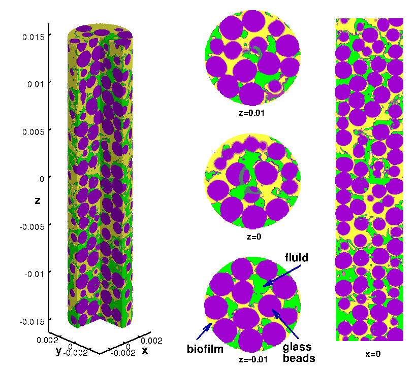
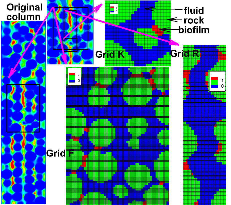
Illustrations in Fig. 1 give an idea about the complexity of the imaging and segmentation process. The voxel grid shown in Fig. 1 is actually a further approximation discussed next.

Figure 1. Geometry of column $\Omega^{1,red2}$ after two voxel reductions. Visible are: the glass beads domain $\Omega_{r}^{1,red2}$, the region $\Omega_{b}^{1,red2}$ occupied by biofilm, and the region $\Omega^{1,red2}_{f}$ occupied by the flowing fluid.

2.2. Grid for flow computations

For the needs of computations we need a covering of $\Omega$ by a computational grid. In particular, the body fitted grids give well resolved local flow results, but require additional overhead, not justified by the accuracy of the conductivities; see [23]. A convenient and practical choice is to use directly the (structured) grid of voxels $\omega_{ijk}$ covering the cylindrical domain $\Omega_{f}$, of size $\phi_{0}^{*}\times 610\times 610\times 2833\times 0.25\pi\approx\mathrm{330M}$. Since some passage between the glass beads may be as small as of single voxel size, we require at least one level of computational grid refinement by dividing each voxel into 8 computational cells. However, the grid of $330M\times 8$ cells calls for a significant computational effort in flow and transport models, and is very challenging even only for pre- and postprocessing, e.g., visualization. Based on our previous experience in [23] we perform therefore some reduction of the original voxel grid by voxel coarsening and/or by cropping $\Omega$ to a rectangular subdomain $\tilde{\Omega}$.

Cropping $\Omega$ to a box-shaped region $\tilde{\Omega}$ is necessary for anisotropic conductivity upscaling, and does not significantly affect the upscaled conductivities as shown later in Sec. 3.2 and Tab. 7.

Voxel coarsening is performed by replacing 8 neighboring voxels $\omega_{ijk}$ with one voxel $\omega^{red1}_{IJK}$ whose property $r_{IJK}$ as in (6) equals that of the majority of $r_{ijk}$ of the aggregated voxels. This corresponds to a rather simple upscaling with which the computational effort decreases by about an order of magnitude. In this paper we used two reduction steps so that the length $h^{red2}_{\omega}=2\times 2h_{\omega}$ of each voxel $\omega^{red2}_{IJK}$ is $h^{red2}_{\omega}=42\cdot 10^{-6}$ m, where “red #” denotes the level of reduction.

After voxel reduction is complete, we assign the computational grid cells denoted by $\Omega_{pqr}$ to be either identical to $\omega^{red2}_{IJK}$, or to their refinement. In particular, for 3D flow simulations we use the computational grid $\mathcal{T}_{h}$ with $h=0.5h^{red2}_{\omega},$ so that 8 computational cells $\Omega_{pqr}$ subdivide one of $\omega^{red2}_{IJK}$. In the coupled transient hydrodynamics-biomass-nutrient (H-BN) simulations we use a coarse grid over small 2D subdomains of $\Omega$ with $h=h^{red2}_{\omega}$.

There is some concern that the strategies of cropping and reduction may reduce the quality of the flow computations. In our previous study in [23] on glass-beads, sandstone, and synthetic geometries, we determined that the voxel reductions, e.g., from $red1$ to $red2$, yield an increase in the conductivities by 7% to 37%. On the other hand, grid refinement decreases the conductivities by 4% to 9% for each consecutive refinement level. In one study of a simple synthetic dataset, six levels of grid refinement led to about 25% reduction in conductivity with respect to that computed for the initial grid. In other words, the increase due to voxel reduction is somewhat mitigated by the decrease due to the grid refinement. Overall, while these effects appear significant, the complexity of the computations on the original voxel geometries for full columns is prohibitive.

2.3. Evaluating effect of biofilm growth without simulations

(a) $\Omega^{1}$, Re=10	(b) $\Omega^{8}$, Re=1	(c) $\Omega^{7}$, Re=0.1

Figure 2. Porosity of fifty slices along the vertical direction ($z$), each slice 56 voxels thick, for the original non-voxel reduced geometries, at $t=0$ (no biofilm), and at $t=T$ (with biofilm). The reduction in porosity due to biofilm is the largest for high flow rates in $\Omega^{8}$ and $\Omega^{1}$. The local variations of porosity in $\Omega_{T}$ appear correlated to those in $\Omega_{0}$.

	solids	voids	dead-end	$\phi$	$\phi_{b}$	$d_{char}$	# cells
	$|\Omega_{s}|$	$|\Omega_{f}|$	$|\Omega_{d}|$				$|\mathcal{T}_{h}|$
$\Omega_{0}^{1}$	7338371	4736720	615	0.3922		1.62	39047712
$\Omega_{0}^{8}$	7222245	4863233	398	0.4024		1.58	40538424
$\Omega_{0}^{7}$	7000612	5034880	1590	0.4182		1.53	41283216
$\tilde{\Omega}^{1}_{0}$	4550752	2815280	553	0.3821		1.88	22517816
$\tilde{\Omega}^{8}_{0}$	4507839	2858193	498	0.3879		1.83	22861560
$\tilde{\Omega}^{7}_{0}$	4442145	2923887	714	0.3968		1.79	23385384
${\Omega}^{1}_{T}$	9918224	2156867	11561	0.1777	0.183	2.82	17162392
${\Omega}^{8}_{T}$	10401329	1684149	16912	0.1379	0.267	2.97	13256024
${\Omega}^{7}_{T}$	8312777	3722715	5682	0.3088	0.108	1.83	29736128
$\tilde{\Omega}^{1}_{T}$	6200908	1165124	16912	0.1559	0.233	3.29	9185696
$\tilde{\Omega}^{8}_{T}$	6428149	937883	51722	0.1203	0.261	3.30	7503064
$\tilde{\Omega}^{7}_{T}$	5231210	2134822	3366	0.2894	0.109	2.05	17078576

Table 2. Geometric information derived from data sets after two voxel reductions. The number of cells $|\mathcal{T}_{h}|$ used in flow simulations for cuboid geometries $\tilde{\Omega}^{c}$ equals $8(|\tilde{\Omega}^{c}_{f}|-|\tilde{\Omega}_{d}^{c}|)$. For $\Omega^{c}$ the voxel-reduction and cell refinement changes this relationship slightly due to the approximation of cylindrical boundaries. The value of $d_{char}$, the ratio of volume of solid matrix to the total area of solids [[5], p119], is given in $10^{-4}$m. Recall that the column numbers correspond to $\Omega^{1}$ (Re=10), $\Omega^{8}$ (Re=1), $\Omega^{7}$ (Re=0.1).

Some information useful for understanding the biofilm growth and the relationship between flow rate and the growth can be found without the flow simulations; see Tab. 2. Here it is useful to develop additional notation to be refined later. We combine $\Omega_{b}$ and $\Omega_{r}$ and call it the “solid” domain $\Omega_{s}$

(7) $$\Omega:=\langle\overbrace{\Omega_{r}\cup\Omega_{b}}^{\Omega_{s}}\cup\Omega_{f}\rangle:=\langle\Omega_{s}\cup\Omega_{f}\rangle,\;\;\phi(\Omega)=\frac{|\Omega_{f}|}{|\Omega|},\;\phi_{b}(\Omega)=\frac{|\Omega_{b}|}{|\Omega|}.$$

The biofilm is excluded from the flow domain, but the biofilm domain may be involved in some transport processes. Note also that $\Omega_{s0}=\Omega_{r}$.

In Tab. 2 we confirm that the porosity $\phi_{0}$ calculated after the voxel reduction step agrees with the experimental value in (1); i.e., the imaging and the voxel reduction preserve the average volume. We also notice that $\phi_{0}(\Omega)$ exceeds that of $\phi_{0}(\tilde{\Omega})$ for cropped geometries; this indicates that there is extra void space near the boundaries of cylindrical enclosures.

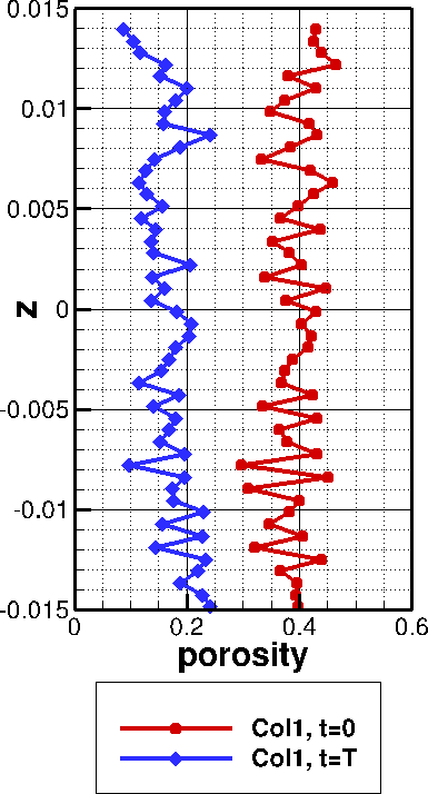
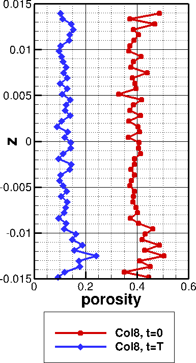
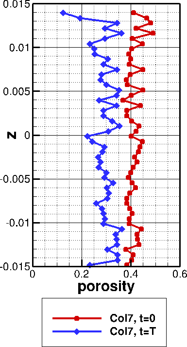
Comparing $\phi_{T}$ to $\phi_{0}$ shows the effect of biofilm growth, and the smallest change is for the slow flow rates. Further insight comes from studying porosity variations in Fig. 2. We see, e.g., that the distribution of biofilm is not homogeneous along columns.

Next, we use a simple algorithm to find the dead-end pores ($\Omega_{d}$); these are assigned by the imaging to $\Omega_{f}$, but are not connected by any path to any of the boundary cells in $\Omega_{f}$, and thus are excluded from the flow. In the current model they are also excluded from transport simulations; we plan to consider including them in the transport model in the future. A large number of dead-end pores indicates a more complex structure of a medium, and in Tab. 2 we see an increase in the number of dead-end pores from $t=0$ to $t=T$, which is most evident for the large flow rates.

We also calculate $d_{char}$, the characteristic length scale, a proxy for grain size, which is calculated as the ratio of volume of a solid matrix to the total area of solids [[5], p119]. We use $d_{char}$ in the Carman-Kozeny correlations discussed later. The change in $d_{char}$ from $t=0$ to $t=T$ indicates changes in geometry which are more pronounced for larger flow rates.

3. Flow simulations and comparison with experiment

Now we discuss the simulations of flow in the columns described in Sec. 2. The imaging and segmentation provide the geometry of $\Omega_{f}|_{t=T}$, $\Omega_{b}|_{t=T}$, and $\Omega_{s}|_{t=T}$ for each column. By “subtracting” out $\Omega_{b}$ from $\Omega_{s}$, we obtain the glass-beads domain $\Omega_{r}|_{t=0}$ as well as the flow domain $\Omega_{f}|_{t=0}$. We can thus perform the flow simulations in $\Omega_{f0}$ and $\Omega_{fT}$ which show the changes in the flow field due to biofilm growth. While we cannot compare the simulated flow field directly to any experiments, we can compare the upscaled conductivities to those obtained in the physical experiment. We provide background for these analyses below.

3.1. Porescale flow model and upscaling

Consider a fixed open bounded domain of flow $\Omega_{f}$, surrounded partially by a solid region $\Omega_{s}$. The flow of liquid (water with nutrients and planktonic cells) in $\Omega_{f}$ is assumed to be viscous, and to obey the steady laminar Navier-Stokes system in $\Omega_{f}$ for velocity $v$ and pressure $p$,

(8a) $$\rho v\cdot\nabla v-\mu\nabla^{2}v = -\nabla p,\;x\in\Omega_{f},$$

(8b) $$\nabla\cdot v = 0,\;x\in\Omega_{f}.$$

We assume no volume forces and ignore gravity. Here $$\mu \rho \Omega_{b}$$ is the viscosity and is the density of the fluid. Other flow models which may include that in are mentioned in Sec. 4.1 but are not implemented here.

The model is complemented by the boundary conditions on $\partial\Omega_{f}$

(8c) $$v|_{\Gamma_{w}\cup\Gamma_{0}} = 0,$$

(8d) $$v|_{\Gamma_{in}} = v_{in},$$

(8e) $$p|_{\Gamma_{out}} = 0.$$

The wall condition (8c) is imposed on internal boundaries $\Gamma_{w}:=\partial\Omega_{f}\cap\partial\Omega_{s}$. The external boundary $\partial\Omega_{f}\cap\partial\Omega$ is divided into the inflow part $\Gamma_{in}$, the wall no-flow part $\Gamma_{0}$, and the outflow part $\Gamma_{out}$, in such a way that $\Gamma_{in}$ and $\Gamma_{out}$ are assigned to a pair of opposite faces of the box enclosing $\Omega$. The inlet velocity $v_{in}$ in (8d) is a given constant, and we use the pressure outlet boundary condition (8e).

To solve (8) numerically, we use the ANSYS software [3], with Finite Volume discretization with grid $\mathcal{T}_{h}$ covering $\Omega_{f}$. With a fixed $\mu,\rho$, and $\Omega_{f}$, the only remaining control parameter is $v_{in}$ and the assignment of the inlet and outlet boundaries.

The results of flow simulations are illustrated in Fig. 3 with the contours of velocity magnitude. They are very complex, especially in geometries with biofilm ($t=T$). In Fig. 3 we see that an increase in the volume of solids due to the appearance of biofilm domain $\Omega_{b}$ between $t=0$ and $t=T$ leads to a substantial reduction of connections among the pores, which, in turn, influences the directions of the flow.

3.2. Upscaling flow results

Once the flow simulation is complete, we upscale its results to get the conductivities $K$ defined for macroscopic pressures $P$ and velocities $V$ by

(9) $$V=K\nabla P=\frac{k}{\mu}\nabla P,\ x\in\Omega,$$

where $K\mathrm{[m^{2}/Pa\cdot s]}$ is the Darcy conductivity, and $k\mathrm{[}m^{2}]$ is the Darcy intrinsic permeability. For small flow rates (9) expresses the macroscopic Darcy’s law, and $K$ is a constant. Our upscaling method, developed in [28] and tested and refined in [22, 24, 25, 35, 23], calculates $V$ and $\nabla P$ via volume averaging of $v,p$ over appropriate portions of $\Omega$ and determines the full tensor $K$ from (9) applied to several flow simulations carried out in independent flow directions. Here we focus on the vertical component of the conductivity $K$ obtained from a single flow simulation in the vertical direction, and we compare it to that obtained in the experiment from pressure transducer values. Additional results on anisotropy and varying flow rates are given in  A.1 and A.2.

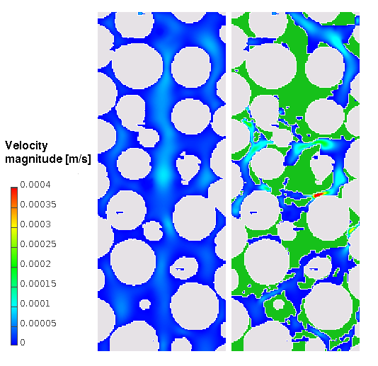a) b)	c)	d)

Figure 3. Visualization of flow simulations in $\Omega^{1}$. Shown are a) the magnitude of velocities in a subsection of $\Omega_{f0}^{1}$ (without biofilm) and b) in $\Omega_{fT}^{1}$ (with biofilm), and c) the streamlines of flow in $\Omega_{f0}^{1}$, and d) the streamlines in $\Omega^{1}_{fT}$. The biofilm is marked in green. The streamlines in c)-d) are colored with the magnitude of velocities applied in a)-b) and showed in the legend to a). Note the nonhomogeneous distribution of biofilm in the vertical direction, and the complexity of flow.

	$\phi^{(a)}$	$10^{8}K^{*}$	$10^{8}K$	$10^{8}K_{CK}$	$10^{8}K_{C}$
Before inoculation, $t=0$, flow rate $500$ml/h
$\Omega^{1}_{0}$	0.3922	97	186.6	84.96	1020.
$\Omega^{8}_{0}$	0.4024	520	197.2	90.76	1001.
$\Omega^{7}_{0}$	0.4182	70.6	227.2	100.4	971.9
With biofilm, $t=T$, at flow rate $500$ml/h
$\Omega^{1}_{T}$	0.1777		10.42	13.15	1408.
$\Omega^{8}_{T}$	0.1379		1.246	6.227	1216.
$\Omega^{7}_{T}$	0.3088		57.84	41.30	1034.

Table 3. Conductivity $K\mathrm{[m^{2}/Pa\cdot s]}$ in the experiment and from simulations carried out on voxel-reduced regions $\Omega^{red2}$. Shown are the values before inoculation, and those computed for geometries $t=T$, at the same flow rate. (Experimentally obtained conductivity ratio at the flow rates characteristic for each column are given in Tab. 4). The right two columns show the Carman-Kozeny $K_{CK}$ and Collins $K_{C}$ estimates of $K$ derived from geometrical information in Tab. 2. Here $K_{CK}=\frac{k_{CK}}{\mu}$ and $K_{C}=\frac{k_{C}}{\mu}$, where $k_{CK}:=0.2\frac{\phi^{3}d^{2}_{char}}{(1-\phi)^{2}}$ is given in [[5], 4.1.20], and $k_{C}:=\phi d^{2}_{char}$ [23]. The porosity (a) from Tab. 2 shown in the left column is well correlated with the computed values.

When comparing the simulated and experimental conductivities we face the following conundrum. Our computations work on fixed geometries and give the same results when repeated; more broadly, averaging of computational results over multiple geometries does not appear natural. On the other hand, the usual experimental practice involves repeated measurements and reporting the averages as well as the associated uncertainty. Should we then compare the averages or rather the individual column values between experiment and simulation ? In this paper we provide and discuss both.

In Tab. 3 we show the values obtained experimentally before inoculation for each column and those obtained from simulations for the same flow rate. Additionally we show the conductivities obtained by simulations for the geometries with biofilm, at the same flow rate as that before inoculation. Next, in Tab. 4 we report the ratio of conductivities at $t=T$ to those at $t=0$; the experimental and computational values in Tab. 4 were obtained for the flow rates characteristic for each column.

First, we note a large variation in the experimental conductivity measurements across the columns. In contrast, the simulated conductivities at $t=0$ were similar to each other across columns, and they correlate well with the porosities derived from imaging. However, the $K$ values overpredict the experimentally obtained conductivities $K^{*}$ for $\Omega^{1}$ and $\Omega^{7}$ and underpredict those for $\Omega^{8}$, with the factors ranging from 2 to about 4. These results appear similar to those in the very recent paper [31] where, depending on the segmentation method and the computational approach, the discrepancy $\frac{K}{K^{*}}\approx$ 13.4 to 2.16. We recall that in [31] the numerical grid corresponds directly to the voxel geometry, but the sample size made of sandstone with different size grains was about 10 times bigger in each direction. The number of cells in the fluid region each direction in [31] was unspecified, but from the information provided we estimate it to be similar to around 30M as in this paper.

In our paper the discrepancy between $K^{*}$ and $K$ can be attributed to several factors. First, the voxel grid for $\Omega_{f}$ is obtained by segmentation, with some of its own uncertainty, and the computational grid is obtained by voxel coarsening and grid refinement, which introduce further approximations. Second, the flow model (as any computational model) in $\Omega_{f}$ gives only approximate results. Next, the upscaling technique can introduce additional small discrepancy as discussed in [28] since the actual REV over which we average is only a subset of the actual flow region; in this REV we avoid spurious computational pressure values near the inflow and outflow boundaries. Additional errors can arise from an imperfect fitting of the slices/sections during the columns reconstruction. Overall, we believe that the agreement between $K$ and $K^{*}$ is quite good, but there is need for further calibration and testing.

Interestingly, as concerns averages, the simulated conductivities are, on average, close to the experimental ones, with a large variation between the individual column values. The analysis of the data along the second column in Tab. 3 gives the average conductivity across the columns $K_{0}^{*}\approx 229.2$ to be close to the simulated conductivities $K_{0}\approx 203.7$, but we do not expect this closeness to be a universal phenomenon.

We provide further information to supplement the values of $K$ and $K^{*}$. In Tab. 3 we list the geometrical estimates $K_{CK}$ and $K_{C}$ which provide almost consistently the lower and upper bounds for $K$ and $K^{*}$. Furthermore, the estimates $K_{CK}$ appear to reflect the changes in geometry due to biofilm clogging consistently with the porosity changes to biofilm clogging, but the $K_{C}$ only provides a stable upper bound. This was already noticed in [23] and indicates the need for further studies towards reduced models.

Next we discuss the conductivity decrease due to biofilm growth, that is, we compare $K_{T}$ and $K_{0}$. In Tab. 4 we show the ratio $K_{T}/K_{0}$ obtained by numerical simulations and $K_{T}^{*}/K_{0}^{*}$ estimated from experiment. The decrease in $K_{T}$ from $K_{0}$ is correlated with a decrease in $\phi_{T}$ from $\phi_{0}$; see Tab. 2 and Fig. 2. The clogging effects are strong for faster flows (Re=1 and Re=10). The biggest reduction in conductivity, of about two orders of magnitude, occurs for $\Omega^{8}$, i.e., the flow rate Re=1. We hypothesize as in [16] that this is due to rapid oxygen consumption at Re$\geq$1 accompanied by (partial) sloughing in $\Omega^{1}$ at Re=10. Similar reduction of conductivity by two or more orders of magnitude due to clogging, was reported by many authors, e.g, [4, 33].

The reduction in $K$ observed in the computations appears similar to that obtained in the experiment, with the closest agreement for Column 7 (Re=0.1). This reaffirms the need for further calibration and experiments, but is promising.

	Re=10	Re=1	Re=0.1
	${\Omega}^{1}$	${\Omega}^{8}$	${\Omega}^{7}$
$K_{T}^{*}/K_{0}^{*}$ (experiment)	0.011	0.092	0.204
$K_{T}/K_{0}$ (simulations in $\Omega^{c}$)	0.056	0.063	0.241
$K_{T}/K_{0}$ (simulations in $\tilde{\Omega}^{c}$)	0.028	0.038	0.205

Table 4. Conductivity reduction $K_{T}^{*}/K_{0}^{*}$ and $K_{T}/K_{0}$ due to biofilm growth.

4. Biomass-nutrient model coupled to hydrodynamics

The growth patterns observed in our experiment as well as in other biofilm studies require a model for the flow coupled to the biomass and nutrient advective-diffusive transport, with biomass growth and nutrient utilization reactions. Biofilm growth occurs by interface expansion, and there is a certain maximum density of cells in a given location that cannot be exceeded. Our Biomass-Nutrient model (BN) is designed to mimick the experiment described in Sec. 2, with the velocity field $v$ computed by the hydrodynamics model (H) (8) described in Sec. 3. The coupled model (H-BN) aims to reproduce the outcome of the experiments.

The main difficulty is to identify what processes take place in different parts of the porespace, and how to resolve the free boundaries between them which change in time. These are overviewed in Sec. 4.1, followed by a literature review in Sec. 4.2. Our mathematical and computational models are made precise in Sec. 4.3 and Sec. 4.4.

In this paper we make three simplifying assumptions. First, we assume that the biofilm region $\Omega_{b}$ can only grow, or remain fixed, and that the change in the flow field is sufficiently slow that solving (H) and (BN) models via a staggered in time approach is reasonable; this is justified by the growth patterns observed in the experiment. Second, we account only for one microbial species (Shevanella oneidensis MR-1) whose mass concentration is denoted by $B(x,t)$, and for one nutrient only (TSB lumped with DO) whose concentration is denoted by $N(x,t)$. Both $B$ and $N$ have units of density. Third, we assume that the region $\Omega_{b}$ is impermeable to the flow. We model the flow in $\Omega_{f}$, and the reactive transport in the liquid region $\Omega_{l}:=\langle\Omega_{f}\cup\Omega_{b}\rangle$ so that (7) is extended as

(10) $$\Omega:=\langle\Omega_{r}\cup\Omega_{l}\rangle:=\langle\Omega_{r}\cup\overbrace{\Omega_{b}\cup\Omega_{f}}^{\Omega_{l}}\rangle:=\langle\overbrace{\Omega_{r}\cup\Omega_{b}}^{\Omega_{s}}\cup\Omega_{f}\rangle:=\langle\Omega_{s}\cup\Omega_{f}\rangle,$$

reminiscent of the overlapping continua at Darcy scale in [14].

4.1. Process description

We describe here the evolution of the domains $\Omega_{r},\Omega_{f},\Omega_{b}$; i.e., the voxel assignment with (6) to one of these domains can change in time.

In the experiment the initial porespace $\Omega_{l0}=\Omega_{f0}$ is inoculated with planktonic biomass which, as we hypothesize, settle at or close to the walls $\Gamma_{w}$ before the pumping of the fluid with the nutrient begins. At the beginning of the pumping, the flow field obeys (8) in $\Omega_{f}=\Omega_{f0}$. The biomass “lives” as planktonic cells (suspended) in the fluid in $\Omega_{f}$ and is subject to the growth and (some) advective–diffusive transport in $\Omega_{l}$. The diffusion of biomass in $\Omega_{l}$ is fairly small, since the size of the cells is large, and the biomass advection is limited, because most cells adhere to the walls of $\Omega_{r}$ or to other cells in $\Omega_{b}$. Over time the biomass forms enough of the extracellular polymeric substance (EPS) to classify the region occupied by the aggregates of the EPS as $\Omega_{b}$ which barium cannot penetrate as in (2); in this region the advective transport essentially ceases, and diffusion is even further inhibited. The nutrient is transported in $\Omega_{l0}$ by advection and diffusion, but its transport in $\Omega_{b}$ becomes inhibited. As biomass grows, its amount eventually exceeds the maximum density possible, and the biomass region has to expand to occupy a larger volume. This occurs by the interface growth, because only the biomass close to the interface has access to the bulk of the nutrient transported in $\Omega_{f}$.

Simultaneously, once the EPS occupies most of $\Omega_{b}$, the fluid cannot penetrate $\Omega_{b}$, and the velocity field needs to be recomputed. Here we treat the part of $\Omega_{b}$ filled with the EPS as impermeable, i.e, part of $\Omega_{s}$. This impermeability assumption can be lifted, and there may be some flow through $\Omega_{b}$. A model for such flow may treat $\Omega_{b}$ as a porous medium or a region of high viscosity [29, 38], but this is outside the present scope.

The evolution of the fluid domains is realized in (H-BN) as follows. The time-staggered loop proceeds in steps $t\to t+\Delta t$, and is initialized with $\Omega_{l0}=\Omega_{f0}:=\langle\Omega\setminus\Omega_{s0}\rangle:=\langle\Omega\setminus\Omega_{r}\rangle$. At time $t$, given the current solid region $\Omega_{s}|_{t}$, we find $v|_{t}$ in $\Omega_{f}|_{t}:=\langle\Omega\setminus\Omega_{s}\rangle$, and set $\Omega_{l}|_{t}=\Omega_{f}|_{t}$, i.e., we initialize $\Omega_{b}|_{t}=\emptyset$. Next we solve (BN) in $\Omega_{l}$ keeping $v|_{t}$ fixed, and we allow for $\Omega_{b}$ to grow. After some $\Delta t$ when the size of $\Omega_{b}$ increases relative to that of $\Omega_{l}$ at the level noticed at the grid resolution, we pause the simulation. We set $\Omega_{s}|_{t+\Delta t}:=\langle\Omega_{s}|_{t}\cup\Omega_{b}|_{t+\Delta t}\rangle$, reset $t+\Delta t\to t$, and start the loop again. Note that we keep track of the biomass in $\Omega_{b}$ at all time steps, even though we do not simulate their evolution once they become part of $\Omega_{s}$.

The mathematical models for the growth of $\Omega_{b}$ are discussed next.

4.2. Biofilm models in literature

The biofilm models divide roughly into those at Darcy scale [14], and those in the bulk fluid [34, 42, 43, 41, 2, 11, 8, 10, 12, 9, 37]. These models account for the advective–diffusive transport and growth of biofilm, each in a different, sometimes not fully comprehensive way. We are not familiar with models which can account simultaneously for the biofilm dynamics coupled to hydrodynamics in complicated porescale geometry.

First, most of the models assume that the diffusion coefficient of biomass $D_{B}$ is very small or zero, since microbial cells are typically large, and $D_{B}$ should be comparable to that of colloids or large particles. The models in [11, 8, 10, 15] make a distinction between bulk liquid in which there are no planktonic cells, and the region in which biomass is nonzero; they further model the biofilm spreading with diffusivity $D_{B}(B)$ depending nonlinearly on $B$, which promotes (infinitely) vigorous spreading of biofilm close to (some) maximum $B^{*}$. This approach of letting $D_{B}$ blow up when $B$ is close to some value $B^{*}$ realizes the maximum constraint, but appears only heuristic, and makes practical numerical computations of this singular model very difficult. On the other hand, in the discrete models based on cellular automata [12, 34] the substrate can diffuse everywhere, with $D_{B}$ reduced by 80% in $\Omega_{b}$. The models calculate the mass in each cell and let the biomass redistribute so that the total amounts never exceed $B^{*}$; however, the results depend on the (heuristic and random) mechanism of redistribution. Next, the work in [42, 43, 41] includes hydrodynamics and advection, but their general approach of phase field models with quite complicated nonlinear dependence of $D_{B}(B)$ requires detailed resolution at the scale of interfaces between $\Omega_{b}$ and $\Omega_{f}$; these appear unfeasible in porescale geometries. The approach in [2] is to account for dynamic mass transfer between planktonic and EPS parts of biomass, supported by a notion of “pressure” (equation) which gives an “advective velocity” that drives the interface $\Gamma_{fb}$ between $\Omega_{f}$ and $\Omega_{b}$; this approach does not account, however, for the external velocity field or for transport within $\Omega_{b}$. A concept similar to this “pressure” is implicitly implied in the aforementioned models in [11, 8, 10], where the interface $\Gamma_{fb}$ appears driven by the gradient $\nabla B$, and the nutrient is subject to transport in $\Omega_{l}$.

In our model (BN) we allow for biomass and nutrient to be transported in the liquid phase $\Omega_{l}$ and for hydrodynamics (H) to be coupled to (BN) in the time-staggered way outlined in Sec. 4.1. Moreover, we implement the constraint of the maximum biofilm density in a novel way described next.

4.3. Biomass evolution and (BN) model

First we recall the well-known growth and consumption rates given by the Monod expressions

(11) $$F(B,N) = k_{B}B\frac{N}{N+N_{0}}=k_{B}Bg(N),$$

(12) $$G(B,N) = -k_{N}B\frac{N}{N+N_{0}}=-k_{N}Bg(N).$$

with $g(N)=\frac{N}{N+N_{0}}$, where $N_{0}$ is the Monod constant. The formula (11) could be easily extended to account for the cell death and removal, but this effect is not significant for the time scale of the experiment discussed here. The positive constants $k_{B},k_{N}$, and $N_{0}$ are assumed known.

The transport model of $B$ and $N$ is a system of advecton–diffusion–reaction equations, with diffusion coefficients $D_{B}$ and $D_{N}$, respectively. It has three new elements in contrast to the literature.

First, we set up the constraint of maximum biofilm density $B^{*}$ to complement these equations

(13) $$B(x)\leq B^{*},x\in\Omega_{l}$$

which is essentially a continuous realization of the biomass spreading mechanism implemented in the cellular automata models [12, 34]. (In practice, (13) is enforced with Lagrange multipliers denoted by $\Lambda$.)

Second, to promote the interface expansion which allows the biomass growth in spite of (13), we set the diffusion coefficient $D_{B}$ to be dependent on $B$; this is a continuous realization of the random spreading mechanism implemented in cellular automata models [12], and is similar to the dependence $D_{B}(B)$ in [11, 8, 10]. In our model however we set $\lim_{B\to B^{*}}D_{B}(B)=D^{*}$, with $D^{*}$ finite but large, while that in [11, 8, 10] was infinite. In $\Omega_{l}:=\langle\Omega_{f}\cup\Omega_{b}\rangle$ the biomass is allowed to diffuse, and we set $\lim_{B\to 0}D_{B}(B)=D_{0}>0$. (In [11, 8, 10], $D_{0}=0$). In our model the diffusion term accounts both for the physical molecular diffusion as well as the mechanism for interface spreading. Our model is also similar to the concept of internal “pressure gradient” in [2] associated with the biomass excess and proportional to the concentration gradient.

Third, to account for both planktonic cells and EPS, the biomass density is partitioned between two components

(14a) $$B=B^{m}+B^{e}$$

where $$B^{m} B^{e}$$ and correspond to the planktonic mobile biomass and the EPS, respectively. Their transport is governed by separate models

(14b) $$\frac{\partial B^{m}}{\partial t}+\nabla\cdot(B^{m}v)-\nabla\cdot(D_{B}\nabla B^{m})$$

$$+\Lambda=-q+F(B,N),\;\;x\in\Omega_{l}$$

(14c) $$\frac{\partial B^{e}}{\partial t}-\nabla\cdot(D_{B}\nabla B^{e})=q,\;\;x\in\Omega_{l}.$$

Here $$\Lambda$$ is the Lagrange multiplier needed to enforce (13).

Thus $B^{m}$ in (14) is allowed to advect with $v$, whereas $B^{e}$ is only allowed to spread and grow from the planktonic cells with rate $q$. It remains to specify how $B^{m}$ depends on $B^{e}$, and this can be done either via a simple first order rate model or an equilibrium model

(14d) $$(RATE)\;\;\;q=\nu_{0}B^{m},{\rm\ or\ }\;\;(EQ)\;\;B^{m}=\nu_{1}B,$$

where $\nu_{0}\geq 0$, and $0\leq\nu_{1}\leq 1$ are constants. Now the (RATE) model is somewhat similar to (some) principles proposed in [2]. The (EQ) model can be seen as an approximation of (RATE) if $\nu_{0}$ is very large. (The case of moderate $\nu_{0}$ will be discussed elsewhere).

In summary, by adding (14b) to (14c) and using (14d) (EQ) and with (14a), we obtain

(15) $$\frac{\partial B}{\partial t}+\nabla\cdot(\nu_{1}Bv)-\nabla\cdot(D_{B}\nabla B)+\Lambda=F(B,N),\;x\in\Omega_{l},$$

(16) $$F(B^{*},N)=0,\;\;\nu_{1}|_{\Omega_{b}}=0.$$

In this model no transport of $B$ (or biomass growth) takes place in $\Omega_{b}$ except for the interface spreading. The interface between $\Omega_{f}$ and $\Omega_{b}$ is defined implicitly while (13) is enforced; this is the crux of the model. Finally, we can define $\Omega_{b}$ in a manner consistent with the intuitive definition (10)

(17) $$\Omega_{b}=\{x:B(x)=B^{*}\};\;\;\Omega_{f}=\{x:B(x)<B^{*}\}.$$

In practice, in the time staggered loop in (H-BN) we set $B_{*}=\nu_{2}B^{*}$

(18) $$\Omega_{b}=\{x:B_{*}\leq B(x)\leq B^{*}\},\;\;\Omega_{f}:=\langle\Omega_{l}\setminus\Omega_{b}\rangle,$$

with $0\ll\nu_{2}\leq 1$; this classifies more biomass as (mature EPS) $\Omega_{b}$ than (17).

It remains to account for nutrient dynamics

(19) $$\frac{\partial N}{\partial t}+\nabla\cdot(Nv)-\nabla\cdot(D_{N}\nabla N) = G(B,N),x\in\Omega_{l}.$$

To account for highly viscous character of $\Omega_{b}$, we modify the diffusivity to depend on $B$, and to be small within and in the vicinity of $\Omega_{b}$; see Sec. 5.

The model (BN) comprises (15) with (13) and (19). It requires boundary and initial conditions for the biomass

(20a) $$\nabla B\cdot n|_{\partial\Omega_{f}\setminus\Gamma_{in}\cup\Gamma_{out}}=0,\;\ B|_{\Gamma_{in}}=0,$$

(20b) $$B|_{\Omega_{l},t=t_{0}}=B_{init}(x),$$

as well as for the nutrient

(20c) $$\nabla N\cdot n|_{(\partial\Omega_{f}\setminus\Gamma_{in})\cup\Gamma_{out}}=0,\;\ N|_{\Gamma_{in}}=N_{in},$$

(20d) $$N|_{\Omega_{s},t=t_{0}}=N_{init}(x).$$

There may be additional interactions between the biomass and the boundaries in (20) which cannot be described by the current no-flux conditions; we plan to consider these in the future.

4.4. Numerical model

We now describe the numerical discretization of (H-BN) in space and time. We realize it in a time-staggered fashion, in a sequence of $M$ macro flow time steps $T_{0}<T_{1}<\ldots T_{J}<\ldots T_{M}=T$. In addition, we set up $N$ micro transport time steps for the (BN) solver, $t_{0}<t_{1}<\ldots t_{n}\ldots t_{N}=T$, with the understanding that $t_{0}=T_{0}=0$, and that each flow time step $T_{J}$ coincides with one of the transport steps $t_{n}$.

4.4.1. Time-discretized coupled (H-BN) model

We set $T_{0}=0,\Omega_{s}(T_{0})=\Omega_{r}$ and proceed as follows for $J=0,1,\ldots$.

1. Given $\Omega_{s}(T_{J})$, define

   (21) $$\Omega_{f}(T_{J}):=\langle\Omega\setminus\Omega_{s}(T_{J})\rangle,$$

   and generate the grid $\mathcal{T}_{h}(T_{J})$ covering $\Omega_{f}(T_{J})$. (The resolution $h$ is kept fixed). Set $\Omega_{l}(T_{J})=\Omega_{f}(T_{J})$.

2. Solve the hydrodynamics model (H) (8) on $\Omega_{f}$ to get the fluid velocity $v|_{T_{J}}$ using the wall boundary conditions (8c) on $\partial\Omega_{f}\setminus\Gamma_{in}\setminus\Gamma_{out}$ and the inflow and outflow conditions (8d), (8e).

3. Project $v|_{T_{J}}$ to a conservative velocity field $v^{H}|_{T_{J}}$ on the grid $\mathcal{T}_{h}(T_{J})$.

4. Use $v^{H}|_{T_{J}}$ as well as the initial conditions $B|_{\Omega_{l},T_{J}}$ as well as $N|_{\Omega_{l},T_{J}}$ to solve the biomass–nutrient (BN) problem on $\Omega_{f}$ for $t\in(T_{J},T_{J+1}]$, where we identify $\Omega_{l}:=\langle\Omega_{f}\cup\Omega_{b}\rangle$ as in (18). The interface $\partial\Omega_{l}\cap\partial\Omega_{b}$ is not tracked explicitly but can be recovered from the knowledge of $B(x)$.

5. Set

   (22) $$\Omega_{s}(T_{J+1}):=\langle\Omega_{s}(T_{J})\cup\Omega_{b}(T_{J+1})\rangle.$$

6. Go to STEP I with $J\rightarrow J+1$.

Details of the algorithm (STEP I…STEP VI) are as follows. STEP I is done via simple postprocessing/remeshing. STEP II, as mentioned before, is done with ANSYS-FLUENT. STEP III is realized using an algorithm described in [6]. STEP IV is realized with the advection-diffusion-reaction model (BN). STEP V requires some bookkeeping and a restart capability in the (BN) model.

As concerns the time stepping, our algorithm requires a new macro time step $T_{J+1}$ to be taken (and a new velocity field $v^{H}$ to be recomputed in STEP II), only when the (new) biofilm phase appears, i.e., $|\Omega_{b}|>0$, observed at the grid resolution. Thus, while a macro time step could be, in principle, as small as the (BN) time step $t_{n+1}$-$t_{n}$, large macro time steps are taken in practice.

Note that the model accounts in (22) only for the increase of the biofilm phase domain, and is not able to describe a change $\Omega_{b}$ that may be due to sloughing. It also ignores the (BN) dynamics in the biofilm region(s) $\Omega_{b}$ after they become a part of $\Omega_{s}$. These features are not a limitation in the present case.

4.4.2. Finite volume/CCFD discretization

The implementation described here is based on the cell-centered finite differences (CCFD), i.e., the finite volume implementation on rectangles, with the well known principles established in [19]. The equivalence of CCFD to the lowest order Raviart-Thomas spaces on rectangles as well as the associated mass conservation properties are described in [30]; see also the details of implementation in irregularly shaped domains in [20, 26].

We first define the finite volume/CCFD discretization, restricting the presentation to 2D. In STEP 1 at every macro time step $(T_{M},T_{M+1}]$, the domain $\Omega_{l}:=\langle\bigcup_{ij}\Omega_{ij}\rangle$, where each grid cell $\Omega_{ij}$ is a rectangle of center $(x_{i},y_{j})$ connected to its neighbors, or with one or more edges on the boundary $\partial\Omega_{l}$.

In what follows we consider the vectors $B^{n}$ and $N^{n}$ of the cell-centered unknowns $B_{ij}^{n}$, and $N_{ij}^{n}$ which approximate $B(x_{i},y_{j},t_{n})$ and $N(x_{i},y_{j},t_{n})$, respectively, for each cell $\Omega_{i,j}\in\mathcal{T}_{h}(\Omega_{l})$; we also consider the vector $\Lambda^{n}$ of the cell-wise Lagrange multipliers.

The fully discrete counterpart of the model (15), (19) under constraint (13) is, given $B^{n},N^{n}$, to solve for $B^{n+1},N^{n+1}$ and $\Lambda^{n+1}$, with $\tau=t_{n+1}-t_{n}$

(23a) $$\frac{B^{n+1}-B^{n}}{\tau}+\nabla_{h}\cdot(B^{n}\nu_{1}v)+D_{B}^{h}(B^{n})B^{n+1}\\ +\Lambda^{n+1}=F(B^{n+1},N^{n}),\;$$

(23b) $$\frac{N^{n+1}-N^{n}}{\tau}+\nabla_{h}\cdot(N^{n}v)+D_{N}^{h}(B^{n})N^{n+1}=G(B^{n+1}_{ij},N^{n+1}_{ij}).$$

This system of nonlinear equations is solved for the vectors $B^{n+1},N^{n+1},\Lambda^{n+1}$; the additional equation binding $\Lambda^{n+1}$ to $B^{n+1}$ is explained in Sec. 4.4.3. Here each of $D_{B}^{h}$, and $D_{N}^{h}$ is a positive definite discrete diffusion matrix, which is equivalent, for constant diffusivity, to the discrete 5-point stencil negative Laplacian $-\nabla_{h}^{2}$. Since in our model diffusivity depends nonlinearly on the solution, the diffusion matrices do so as well; we use averaging on the cell edges and time-lagging. The operator $\nabla_{h}\cdot$ handles the advective fluxes across the edges by (first-order) upwinding.

In (23) we evaluate the advection term $+\nabla_{h}\cdot(B^{n}\nu_{1}v)$ explicitly in time, as in the framework of operator splitting scheme as in [39]. This requires

(24) $$\tau\leq\tau_{CFL}:=0.5\min_{ij}\max(h_{x}/v_{x},h_{y}/v_{y})|_{\Omega_{ij}},$$

where the grid dimensions $h_{x}h_{y}=|\Omega_{ij}|$ are as in Sec. 2.2, and where the velocities $v_{x},v_{y}$ are the maximum across the left and right, and bottom to top, edges of $\Omega_{ij}$, respectively. In [39, 27] the advection is followed by reaction and next by diffusion. In our scheme we first handle (explicit) advection for both components, and then combine the reaction and diffusion steps, while accounting for (13), and time-lagging the diffusion coefficients. In fact, we first solve (23a) for $B^{n+1}$ using the time-lagged value of $N^{n}$ in the reaction term, and then solve (23b) using that new value.

4.4.3. Implementing the inequality constraint

The main challenge of the biofilm model is the presence of the free boundary $\Gamma_{fb}=\partial\Omega_{f}\cap\partial\Omega_{b}$ between the fluid and biofilm, i.e., the real interface “seen” by the imaging equipment thanks to the barium-based agent. Accounting for $\Gamma_{fb}$ is essential to describe biofilm growing volumetrically through the interface. In our model $\Gamma_{fb}$ is defined implicitly by (17) along with (13).

To realize (13) as in obstacle problems and variational inequalities [18, 36], one introduces the Lagrange multiplier $\Lambda^{n+1}$ which is a vector of dimensions identical to those of $B$. Then we rewrite (13) as the nonlinear complementarity constraint, where at every grid point

$$\forall\Omega_{i,j}\in\mathcal{T}_{h}(\Omega_{l}),\;\;\left\{\begin{array}[]{l}\Lambda^{n+1}_{ij}\geq 0,\\ B^{*}-B^{n+1}_{ij}\geq 0,\\ \Lambda^{n+1}_{ij}(B^{*}-B^{n+1}_{ij})=0.\end{array}\right.$$

This constraint can be efficiently implemented using the “$\min$” function and is equivalent to

(26) $$\min(\Lambda^{n+1}_{ij},(B^{*}-B^{n+1}_{ij}))=0,\;\;\forall\Omega_{i,j}\subset\Omega_{l}$$

In short, the Lagrange multiplier is nonzero in the so-called active set of gridpoints where $B_{ij}=B^{*}$, i.e., in the (sub)set of $\Omega_{b}$.

The equations (23a)–(23b) with (26) can be solved with Newton’s method. Since the function “$\min$” is not differentiable everywhere, this version of Newton’s method is called semismooth, and is known to be convergent at almost the optimal rate [36], provided the Jacobian is never singular. We can prove the latter based on some further time-stepping constraints; this along with other mathematical and numerical analyses is discussed in the companion paper [21].

5. Numerical simulations of (H-BN) model

In this Section we present numerical simulations to test the (H-BN) model in the conditions similar to the experimental setup of Sec. 2. The simulations help to gain additional insight unavailable from the experiment alone.

Figure 4. Computational 2D domains for (H-BN) and (BN) simulations $\Omega^{K},\Omega^{R},\Omega^{F}$ are extracted from the cross-sections of $\tilde{\Omega}^{1}$ along the $z$ axis; note the resemblance of $\Omega^{F}$ to the crosssection shown in Fig. 1. In $\tilde{\Omega}^{1}$ shown is the velocity magnitude between glass beads. The domains $\Omega^{K}_{r},\Omega_{r}^{F},\Omega_{r}^{R}$ were slightly conditioned in order to assure good percolation. The location of domains in $\tilde{\Omega}^{1}$ is indicated by the arrows connecting the upper left corner of each domain. In $\Omega^{K}$ the arrows indicate $\Omega_{f}$ (blue), $\Omega_{r}$ (green), and $\Omega_{b}$ (red).

Ideally, we would set up time-dependent simulations with enough resolution to mimick the experimental setup. Unfortunately, this is not feasible. A quick estimate of the time step required to simulate (BN) with the flow from hydrodynamics model (H) corresponding to $v_{in}=10^{-5}$m/s, with grid size of approximately $5\cdot 10^{-6}$m, shows that the time step for explicit advection by (24) is $\tau_{CFL}\approx O(1)$sec. (Locally the velocities can be larger than $v_{in}$ which reduces the time step further). Even with an implicit advection solver, the time steps must still correspond to the characteristic time for diffusion and biochemical reactions, and thus are limited. Now, at each time step we have to solve (at least) two linear systems, each of around $5M$ cells; further difficulties are associated with the nonlinearity of the problem which requires even more delicate time stepping. Therefore simulation of $T=11$ days of biofilm growth in the full column was not possible in this study.

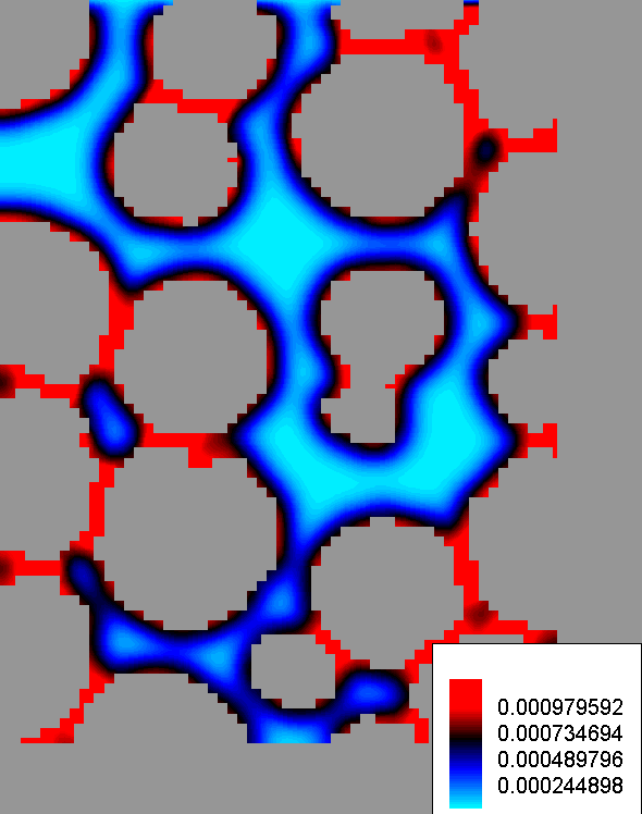
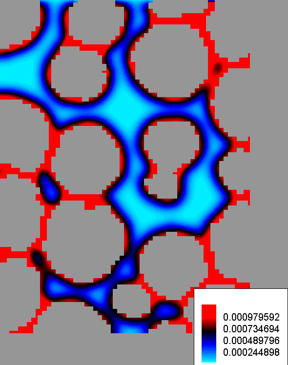
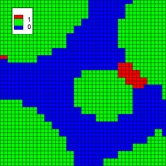
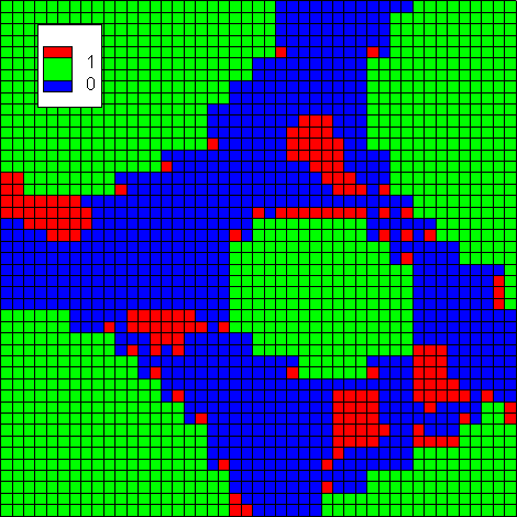
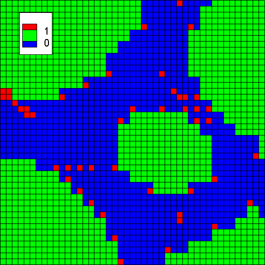
We limit ourselves instead to a focused study aimed to demonstrate the robustness of the (H-BN) solver, and to the illustration how the porescale geometries change depending on the model parameters. We use only 2D geometries, which are subsets (of a vertical slice) of $\Omega^{1,red2}$ organized as three cases $\Omega^{K},\Omega^{R},\Omega^{F}$; see Fig. 4. In addition, we use $v_{in}\leq 10^{-3}$ because of (24); this excludes the fastest flow rate used in the experiment. We also double the reaction rates given in the literature in order to promote significant biomass growth within a small $T$ of simulations. Depending on the case, we simulate only $T=1$ day, or $T=2$ days; these times are usually sufficient for the clogging to completely block the flow paths.

In addition to the coupled (H-BN) model we also consider the simulation setup referred to as (BN) in which the velocity values computed by the model (H) at $t=0$ are fixed, and are not recomputed.

We present the simulation parameters in Tab. 5. The top rows include basic parameters common to all the test cases. Further parameters are listed in bottom rows, along with additional simulation cases enclosed in brackets, e.g., the case K_BA uses geometry $\Omega^{K}$ and parameters indicated by [BA].

(A)	Growth constant	$k_{B}=1.8\cdot 10^{-5}$/sec
(B)	Utilization constant	$k_{N}=1.8\cdot 10^{-4}$/sec
(C)	Monod constant	$N_{0}=1.6\cdot 10^{-3}\mathrm{kg/m^{3}}$
(D)	Nutrient diffusivity	$D_{N}(x)/D_{m}=2\chi_{\Omega_{f}}(x)+0.1\chi_{\Omega_{b}}(x)$
(E)	Biomass diffusivity	$D_{B}(x)$, see (27)
(F)	Biofilm phase parameters	$\nu_{2}=0.9,B^{*}=0.0012\mathrm{kg/m^{3}}$, $B_{*}=\nu_{2}B^{*}$
(G)	Boundary data	$N_{in}=0.01\mathrm{kg/m^{3}}$, $B_{in}=0$
(H)	Initial nutrient	$N_{init}(x)=0$
(I)	Initial biomass	$\nu_{B}B_{0}=0.2$,  [$\nu_{B}B_{0}=0.1$ (SI)]
(J)	Inlet velocity	$v_{in}=10^{-5}$m/sec
		[$v_{in}=10^{-4}$ m/sec (FA), $v_{in}=10^{-3}$ m/sec(VFA)]
(K)	Viscous factor	$\nu_{1}=0$, [$\nu_{1}=1$ (BA)],
		[$\nu_{1}=0.5$ (BAP), $\nu_{1}=0.01$ (BAS)]

Table 5. Model and simulation parameters. (A-C) adapted from [41, 14] where we double $k_{B},k_{N}$. $D_{m}=10^{-9}\mathrm{m^{2}/s}$ is the standard molecular diffusivity in water. (D-F) are chosen based on [11, 41]. (G-H) and (I-K) resemble the experimental setup. (I-K) vary between simulation sets as indicated.

The initial biomass is set to be spread in randomly chosen cells in the region $\Omega_{I}$ adjacent to the rock liquid interface $\partial\Omega_{r}\cap\partial\Omega_{l}$. Specifically, enough grid cells $\Omega_{ij}\subset\Omega_{I}$ adjacent to $\partial\Omega_{r}\cap\partial\Omega_{l}$ are selected to cover a desired fraction $\nu_{B}$ of $\Omega_{I}$ with $B_{init}(x)=\nu_{B}B_{0}\cdot 0.0003\mathrm{kg/m^{3}}$ for $x\in\Omega_{I}$, where $\nu_{B}B_{0}$ is a parameter; this choice provides comparable initial conditions in the different cases $\Omega^{R},\Omega^{K},\Omega^{F}$.

Diffusivity of biomass given in Tab. 5 is given by

(27) $$D_{B}(x)/D_{m}=.0001\chi_{\Omega_{f}}(x)+l(B)\chi_{\Omega_{b}}(x),$$

where $l(B)$ is a linear function which increases from $.0001$ at $B=B_{*}$ to tenfold $.001$ at $B=B^{*}$. This choice of $D_{B}$ is motivated by [11, 8, 10] as well as the phase-field models in [41, 42]. Note that when $B=B^{*}$, the diffusion ceases within most of $\Omega_{b}$ due to $\nabla B^{*}=0$, but the interface growth is promoted to the outside of $\Omega_{b}$.

5.1. Simulation results: biomass growth and flow patterns

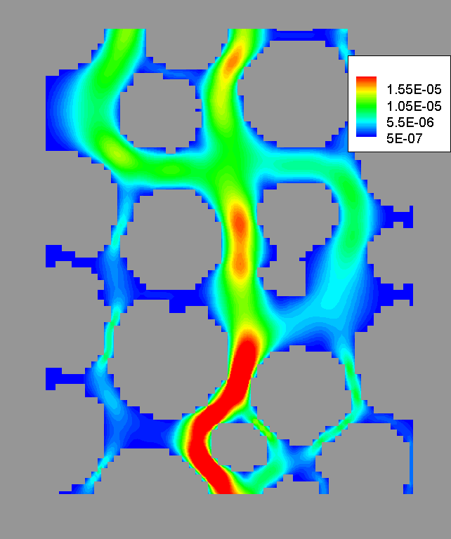
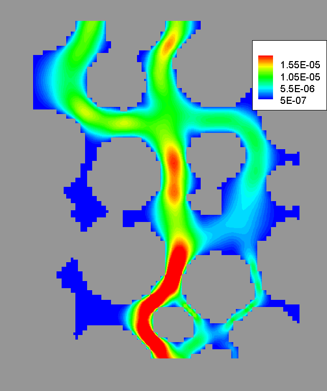
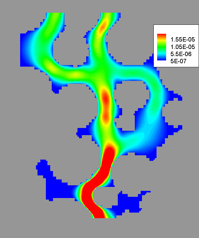
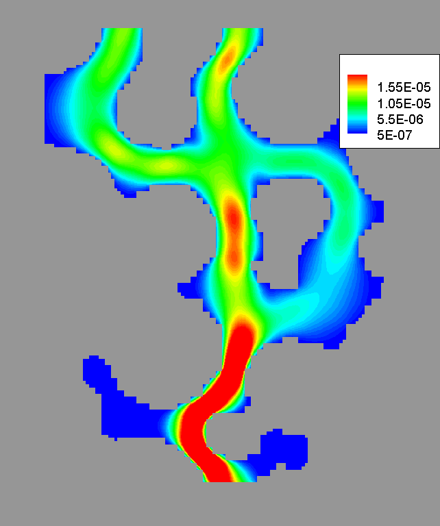
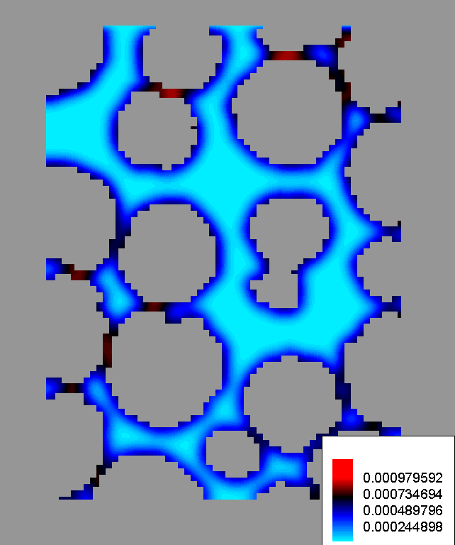
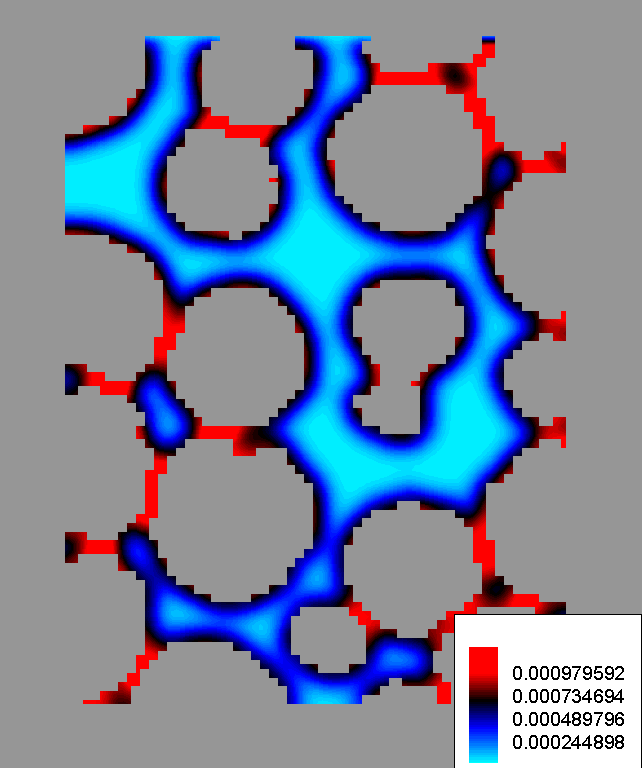
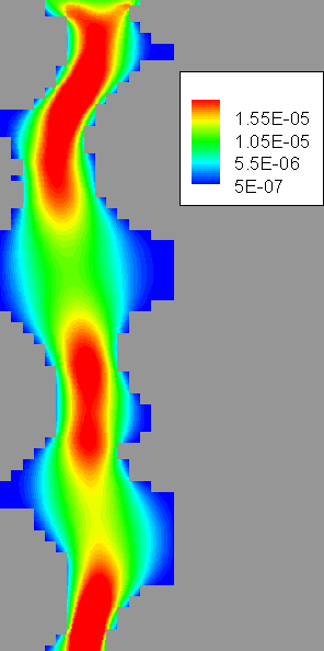
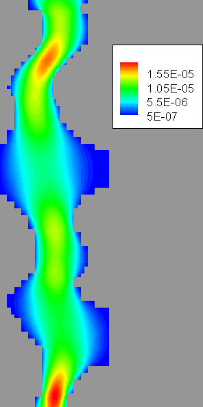
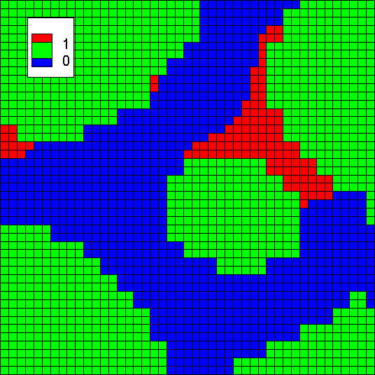
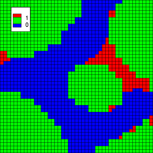
For all the domains $\Omega^{F},\Omega^{K},\Omega^{R}$ we set up the flow in the simulations to be from top to bottom, i.e., the inflow boundary is the top boundary; plots are shown in Fig. 5, 6, 7. As the simulation progresses, the biomass grows and the biofilm phase appears at a certain time indicated in Tab. 6 which varies from 15h to 18h. The regions $\Omega_{b}$ (and $\Omega_{s}$) grow as shown in rows 4–5 of Tab. 6. For some data sets the time 24h is more than enough for clogging to occur, and the simulation stops. (The actual experiment discussed in Sec. 2 continues much longer in a larger domain with smaller initial data and smaller reaction rates.)

	$\Omega^{K}$	$\Omega^{R}$	$\Omega^{F}$
Grid	46$\times$46	32$\times$120	114$\times$152
$|\mathcal{T}_{h}(\Omega)|$	2116	3840	17328
Time $T$	24h	24h	48h
$|\Omega_{s0}|$	1180	1496	9404
$|\Omega_{sT}|$, (BN)	1500	3278	13550
$|\Omega_{sT}|$, (H-BN)	1553	3491	13975
Computational effort(a) (wall clock)	2h	3h	10h
Biofilm phase apppearance (BN)	17h	15h	15h
Biofilm phase apppearance (H-BN)	17h	15h	15h
Time clogging (BN)	23h	24h	30h
Time clogging (H-BN)	28h	24h	29h

Table 6. Simulation results for (H-BN) and (BN) simulations. (a) Run time for the MATLAB implementation of (BN) model

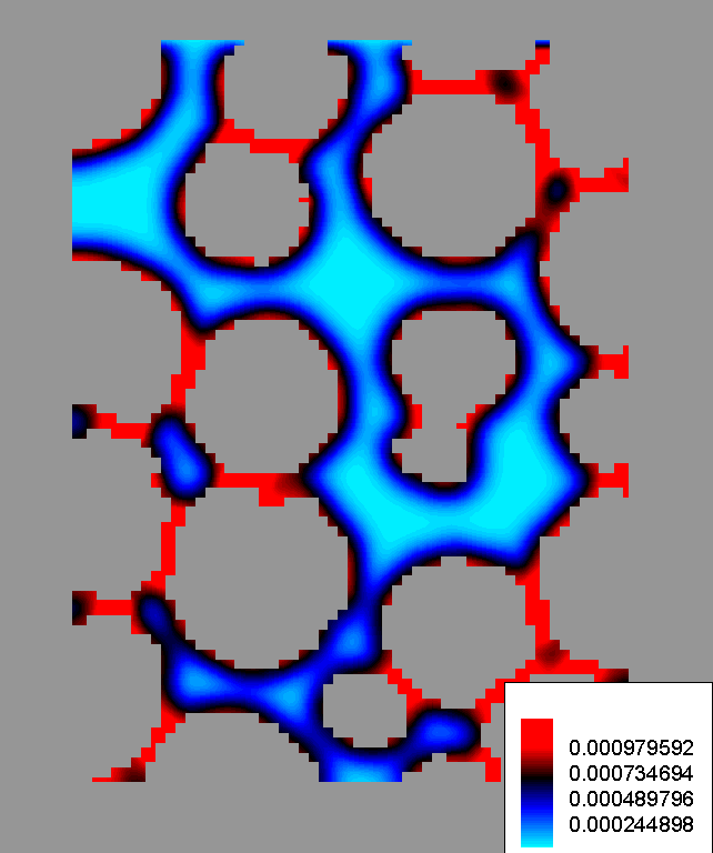
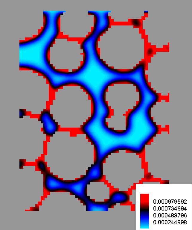
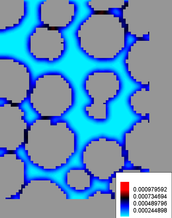
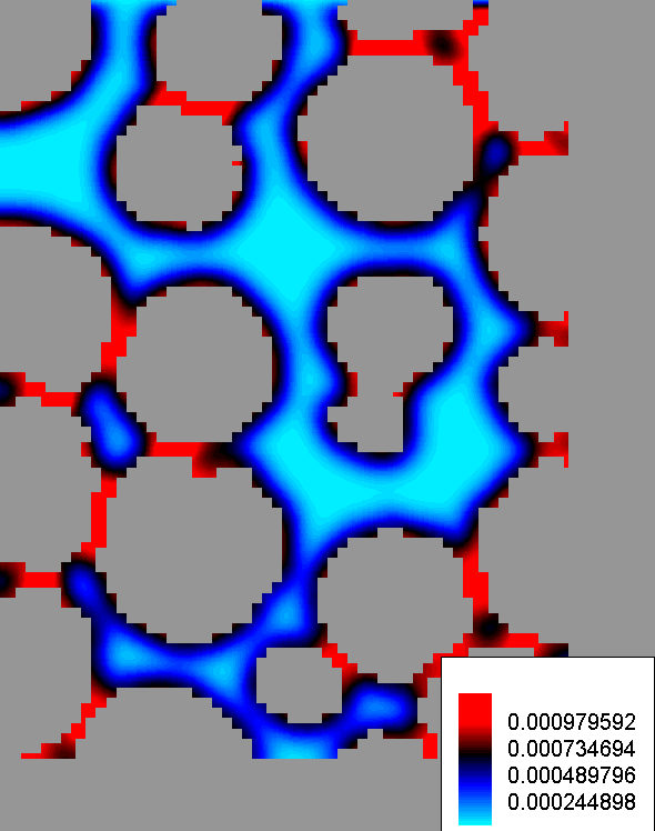
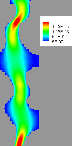
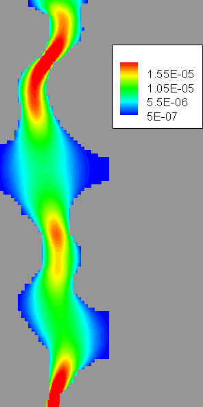
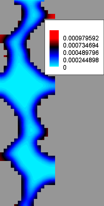
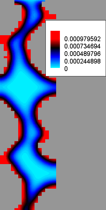
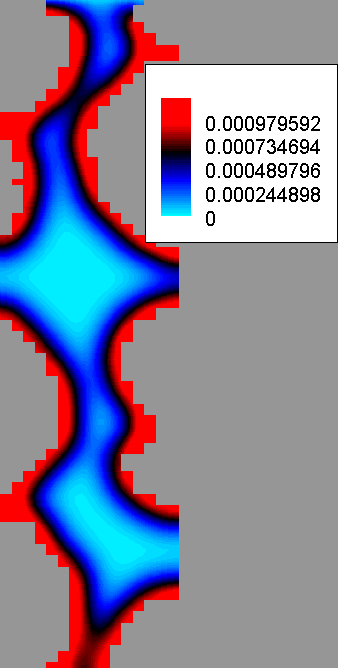
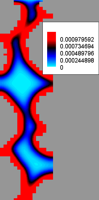
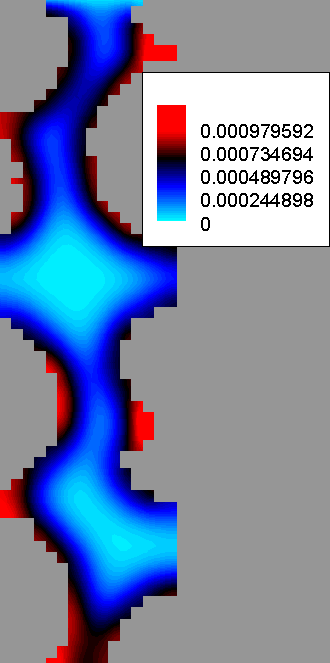
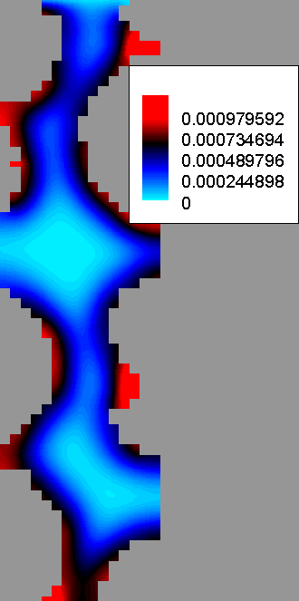
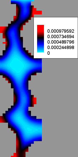
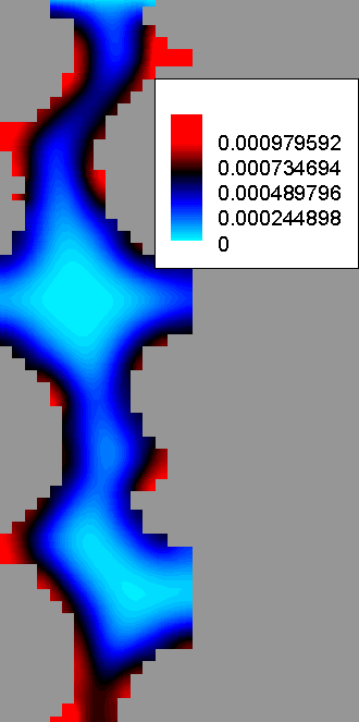
First we discuss the overall patterns of biomass growth. In particular, consider Fig. 5 for the case $\Omega^{F}$ and Fig. 6 for $\Omega^{R}$. With substantial initial amount $\nu_{b}B_{0}=0.2$, we see that the growth appears to take place preferentially in the more narrow and horizontally aligned passages, away from the flow in $\Omega^{F}$, but it occurs essentially uniformly along the walls in $\Omega^{R}$. Overall, the patterns in these figures are qualitatively similar to those obtained in imaging the biofilm domain as in Fig. 1, but clearly we cannot hope to match the images from experiment pointwise, e.g., without knowing the exact distribution of initial biomass.

Now we address the importance of recomputing velocities, i.e., as in the fully coupled (H-BN) model, where velocities are recomputed each time the domain $\Omega_{f}$ changes, compared to the (BN) model, in which the velocities are computed only once at $t=0$. The velocity profiles in the changing domain are shown in Fig. 5, 6, and the profiles clearly depend on the domain. However, while the biomass amount shown in Fig. 5 has a somewhat different profile between (H-BN) and (BN) models, this difference is hard to notice at the time scale and spatial resolution used in our simulations. The differences are better seen in Tab. 6 as well as in cumulative plots in Fig. 8 discussed below.

t=10h	t=18h	t=20h	t=22h

Figure 5. Velocity computed in (H-BN) simulations (top) show a significant change of the flow domain over time. Biomass growth for $\Omega^{F}$ with (H-BN) model (middle) and (BN) model only (bottom) show that most of the growth occurs away from main flow pathways. However, there is a relatively small difference in the distribution of planktonic cells between (BN) and (H-BN) models.

Next we assess the effect of a particular initial distribution of biomass; see Fig. 6. For a larger initial biomass amount with $\nu_{B}B_{0}=0.2$, the simulated biomass growth (not shown) corresponding to the different initial conditions appears very similar. With a smaller amount and $\nu_{B}B_{0}=0.1$, the growth shown in Fig. 6 is more randomly distributed, but the consistent pattern of biofilm growth away from the flow paths is preserved; this is likely due to the placement of initial biomass always next to the walls, even if it is initiated in slightly altered locations.

t=10h	t=18h	t=20h	t=22h
t=12h	t=18h	t=20h	t=24h
$|v|$ (top) and $B$ in (H-BN) simulations
$B$ at t=32h simulated from random initial data

Figure 6. Velocity profiles in $\Omega_{f}^{R}$ (top) and biomass amount (middle) in (H-BN) simulations for $\Omega^{R}$; note the domain change of $\Omega_{f}^{R}$. Bottom: For smaller initial amount in the case [R_SI], the biomass profiles at $t=32h$ differ only slightly between the different random distributions of initial biomass.

5.2. Effect of flow rates and biomass advection parameter $\nu_{1}$

(a) $\Omega^{K\_VFA}$	(b) $\Omega^{K\_FA}$	(c) $\Omega^{K}$	(d) $\Omega^{K\_BAS}$	(e) $\Omega^{K\_BA}$
$v_{in}=10^{-3}$	$v_{in}=10^{-4}$	$v_{in}=10^{-5}$	$v_{in}=10^{-5}$	$v_{in}=10^{-5}$
$\nu_{1}=0$	$\nu_{1}=0$	$\nu_{1}=0$	$\nu_{1}=0.05$	$\nu_{1}=1$

Figure 7. The evolution of domain $\Omega^{K}_{f}$ with (H-BN) simulations depending on the overall flow rate and the advection parameter $\nu_{1}$ in the model (15). The cases (a-c) show faster biofilm growth for faster flow reates which seems to agree with the experimental findings. The cases (c-e) show the ability of the model to allow the biomass to advect with the flow.

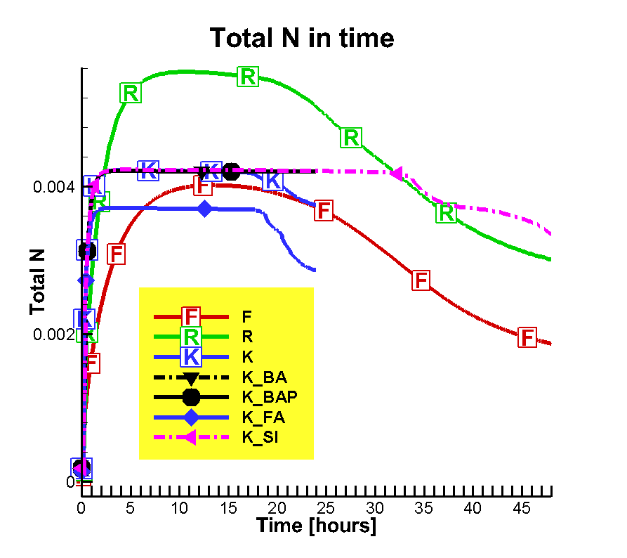
Now we discuss the dependence of the growth on the flow rates and on the modeling assumption concerning the biomass advection. In Fig. 7 (see also later cumulative values in Fig. 8) we compare the base case of $v_{in}=10^{-5}$ in $\Omega^{K}$ (see row J in Tab. 5) with that when $v_{in}=10^{-4}$ (K_FA), or $v_{in}=10^{-3}$ (K_VFA). The evolution of $\Omega_{f}^{K}$ for these cases indicates that the biofilm phase growth appears concentrated in the regions of more stagnant flow, and that it increases with higher flow rates; this seems to agree with the experimental findings.

Second, we simulate cases in which the biomass advection is allowed; this is controlled by the (ad-hoc) parameter $\nu_{1}$ from (15). We compare the base case where $\nu_{1}=0$ (no biomass advection) to the cases with $\nu_{1}\neq 0$ (some biomass advection); the latter cases are listed in row (K) of Tab. 5 and denoted by (K_BA), (K_BAP), (K_BAS), respectively. In the extreme case of large $\nu_{1}\approx 1$ [K_BA], the biomass behaves like colloids, and its growth and transport is very different from that for $\nu_{1}=0$ (K). The intermediate case (K_BAS) shows similar effects which (superficially) resemble sloughing of biomass.

The experiment suggests that including advection and sloughing is important, but there is no imaging data to pinpoint exactly the processes involved, and to help calibrate $\nu_{1}$. On the other hand, the models of sloughing available in the literature describe detachment but cannot yet describe simultaneously the interactions of sloughed biomass with the walls of the porous medium. While our model results associated with $\nu_{1}$ are promising, this aspect needs further work.

5.3. Cumulative values

The plot of cumulative values of nutrient and biomass dynamics is shown in Fig. 8. First, we notice a very quick saturation of the domain with the nutrient. This is consistent with the large (vertical) flow rates combined with the diffusion for horizontal transport, so that the entire domain appears essentially filled with nutrient within at most 2h for $v_{in}=10^{-5}$m/s. The simulations in the (small) domains $\Omega^{F},\Omega^{K}$, and $\Omega^{R}$, suggest that the biomass growth after this initial time is not nutrient limited. In addition, we notice that about the time the biofilm phase forms, the nutrient’s consumption is substantial, in spite of being replenished through the advection. In contrast, in the much larger spatial domains in the experiment, a much longer time is needed for the nutrient to penetrate the entire domain, and the optimal growth is for $\Omega^{8}$ and the intermediate flow rate.

Second, we see in Fig. 8 that the exponential growth of biomass tapers off within a few hours after the biofilm phase appears (when $B^{*}$ is attained). This is a known phenomenon, since biofilm tends to grow mostly through interfaces. In our porescale simulations the growth through interfaces is however more limited than in the bulk liquid, due to the presence of additional rock interfaces.

Further, the porosities and upscaled conductivities decrease due to biofilm growth, but the decrease follows a different pattern for each of the domains $\Omega^{F}$, $\Omega^{R}$, and $\Omega^{K}$, and for some model parameters. Since the porosity is a proxy for biomass growth, the porosity–conductivity plots give the reduced model for dependence of $K=K(B)$. The case of $\Omega^{R}$ is the smoothest, and it corresponds to about cubic decrease in conductivity as a function of porosity; this is consistent with the “pipe-like” character of flow in $\Omega^{R}$. For $\Omega^{F}$ the conductivities decrease in steps corresponding clearly to the clogging of minor paths. Finally, the cases [K_BA] and [K_BAP] in which the biomass is allowed to advect stand out as those corresponding to the most irregular geometry modifications. More studies over larger REV are needed to fully understand these dynamic effects.

Figure 8. Cumulative and average values obtained in the simulations. Left top: total nutrient evolution. Left bottom: porosity vs conductivities; each marker corresponds to a different time snapshot, and some markers are omitted. Right: evolution of total and maximum biomass (top) and the zoomed in difference between (BN) and (H-BN) models (bottom).

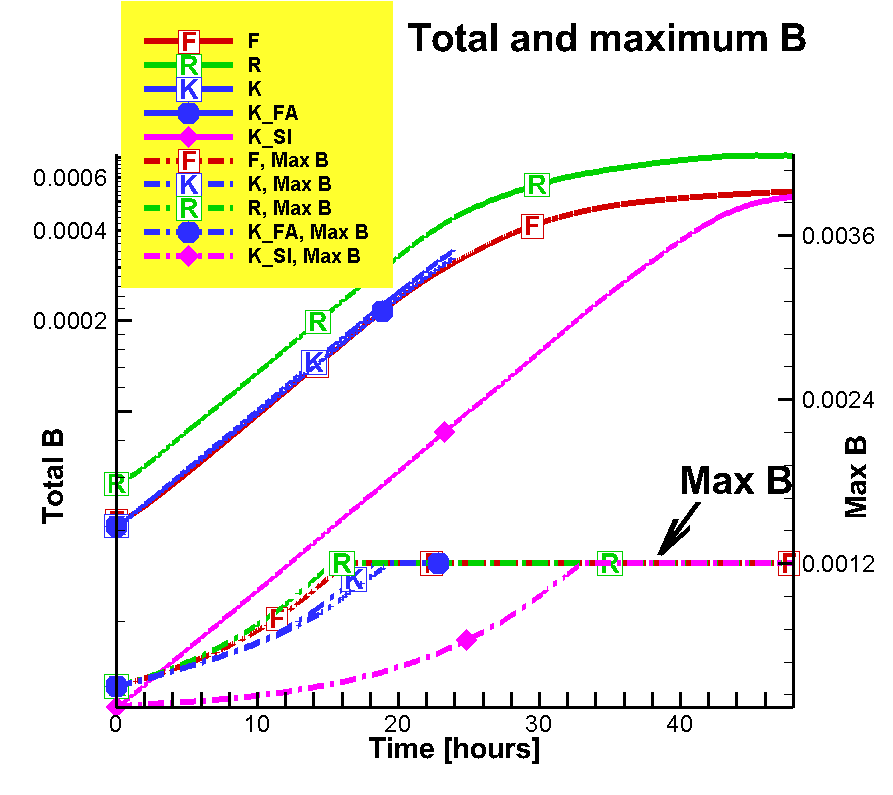
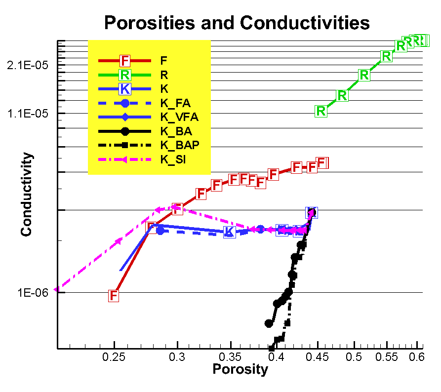
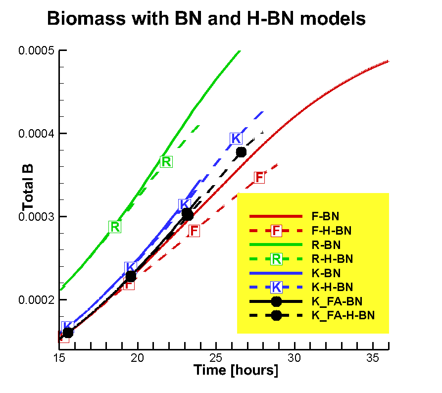
5.4. Further discussion of simulation results

The simulations and the model are not designed to match the experiment because of the the tremendous computational effort that would be required at the time and spatial scales involved. Our results indicate that the (H-BN) model is robust and gives results which qualitatively agree with the images obtained in the experiment. However, the specific growth pattern is strongly dependent on the geometry and on the initial conditions, and one should not expect a perfect match.

In particular, the experimental results in Fig. 2 show that biomass tends to accumulate generally closer to the inlet than to the outlet; this can be explained by the relative availability of nutrient, or by biomass advection [4]. However, our simulations (on small domains) do not show that the growth is nutrient limited but rather that it continues preferentially in narrow passages. On the other hand, the choice of $\nu_{1}$ appears important as it promotes the relocation of biomass towards the outlet. Finally, our experiments show the dependence of the growth patterns on the flow rates, even for the limited set of $v_{in}$ chosen, but further comprehensive parameter studies are needed. Also, one should perhaps consider some stochastic extensions of the model and simulations to handle the unknown initial conditions.

6. Conclusions

Valuable insight comes from combining imaging, experiments, and numerical simulations and visualization. The combined pore-scale flow experiments and simulations undertaken in this paper allow the study of the impact of biomass growth on both the micro-scale flow as well as on the core-scale parameters such as porosity and conductivity.

The (H) flow model and upscaling appear robust. We see very good qualitative agreement and close quantitative agreement between the experimental and the simulated conductivities. With the simulations, we obtain detailed understading of flow patterns which is unavailable experimentally; we also obtain fully anisotropic and heterogeneous conductivities. Also, simple geometrical correlations provide useful bounds for conductivities in regular geometries.

The biomass-nutrient (BN) model we proposed and the coupled (H-BN) model are promising but need more work. Further refinement in close contact with experimentalists is needed to describe the flow in $\Omega_{b}$ as well as the EPS formation and interface growth, sloughing, the movement of planktonic cells, and the taxis that attract the cells to interfaces. In particular, the model parameter $\nu_{2}$ could be correlated to the estimates of interfacial area. Next, so far our simulations have shown a mild dependence of the growth on the flow rates and the associated nutrient (DO) availability while a stronger one was hypothesized based on the experiment in [16, 17]; we want to calibrate the model better in order to understand this fundamental feature. Furthermore, we plan to improve the efficiency of the (BN) model, e.g., via parallelization, to enable larger 3D domain studies. Finally, due to the prohibitive complexity of (H-BN), it is currently impractical to conduct substantial parameter studies, and we intend to explore further various reduced models.

While more work is needed, an improved and calibrated (H-BN) model can be eventually used in a predictive mode to test various scenarios, a task that cannot be accomplished easily through experimentation of this complexity.

Appendix A Anisotropic conductivities and at large flow rates

A.1. Computations of full tensor on cropped rectangular domains

	$10^{8}K_{xx}$	$10^{8}K_{yy}$	$10^{8}K_{zz}$	$10^{8}K$	$10^{8}K_{CK}$	$10^{8}K_{C}$
No biofilm, $t=0$
$\tilde{\Omega}^{1}_{0}$	180.8	186.2	227.6	203.4	102.7	1342.
$\tilde{\Omega}^{8}_{0}$	186.2	195.8	273.1	213.0	104.4	1300.
$\tilde{\Omega}^{7}_{0}$	200.2	212.5	234.9	235.0	110.2	1279.
With biofilm, $t=T$
$\tilde{\Omega}^{1}_{T}$	6.845	7.310	7.791	5.965	11.49	1685.
$\tilde{\Omega}^{8}_{T}$	1.716	1.199	0.949	0.811	4.882	1305.
$\tilde{\Omega}^{7}_{T}$	57.19	59.33	55.37	48.14	40.28	1215.

Table 7. Conductivities $K\mathrm{[m^{2}/Pa\cdot s]}$ from simulations in cropped voxel reduced regions $\tilde{\Omega}^{c,red2}$ at $t=0$, and $t=T$, and $v_{in}=10^{-5}$m/s. The left columns show the diagonal components of the anisotropic tensor upscaled from three independent simulations. The middle column shows the conductivity $K$ in $z$ direction computed from a single simulation. The right two columns show the estimates $K_{CK}$ and $K_{C}$ of $K$ derived from geometrical information in Tab. 2.

Our anisotropic nonlinear upscaling method developed in [28] and tested and refined in [22, 24, 25, 35, 23] calculates $V$ and $\nabla P$ via volume averaging of $v,p$ over appropriate portions of $\Omega$, and determines $K$ from (9). The calculation of all components of the full tensor $K$ (which needs not be diagonal) requires three computational experiments in which we vary the assignment of inflow and outflow boundaries to align roughly with the $x$, $y$, and $z$ directions, but requires rectangular shape of the domain. We supplement the data in Tab. 3 calculated for the full cylindrical columns $\Omega$ with additional information in Tab. 7 on the anisotropic conductivities calculated for cropped domains $\tilde{\Omega}$. We present $K_{xx},K_{yy},K_{zz}$ only and skip the off-diagonal components. We see that $K$ reported in Tab. 7 has generally a somewhat larger value than that in Tab. 3, i.e., full columns $\Omega$ have smaller values of $K$ than the subregions $\tilde{\Omega}$ for $t=0$ but the opposite is true for $t=T$. While the latter appears naturally correlated to the associated difference in porosity between $\Omega_{T}$ and $\tilde{\Omega}_{T}$, the former could be explained by the difference in the flow paths between cylindrical and box shaped regions. Second, while $K$ computed from $\Omega_{f0}$ is essentially isotropic, that for $\Omega_{fT}$ is not, but there is no consistent pattern of anisotropy. This indicates a strong nonuniform increase in resistivity to the flow due to the biofilm growth.

A.2. Computations with varying flow rates

In addition to conductivities reported in Tab. 3, Tab. 7 and Tab. 4, we performed computational experiments for a wide range of flow rates; see Tab. 8. As is well known, the nonlinear effects in the flow appear typically at flow rates corresponding to around $Re$=$1$, even though this nondimensional number may have ambiguous definitions at the porescale. At macroscale, the onset of inertia effects is manifested by a decrease in the conductivity defined by (9) [28, 23]. With the data in Tab. 8 we confirm the presence of a linear flow regime below $v_{in}=10^{-3}$ m/s (e.g., $Re$=$1$). The value $v_{in}=10^{-3}$ m/s marks the onset of inertia effects with a decrease in the conductivities. Nonlinear effects become visible for $v_{in}=10^{-2}$ m/s ($Re$=$10$), and become even more pronounced at $v_{in}=10^{-1}$ m/s ($Re$=$100$).

Re	$\tilde{\Omega}^{1}_{0}$	$\Omega^{1}_{0}$	$\tilde{\Omega}^{1}_{T}$	$\Omega^{1}_{T}$
0.1	203.4	199.3	5.965	10.76
1	202.8	198.8	5.945	10.75
10	185.3	186.6	5.327	10.42
100	85.67	96.15	2.142	6.803
	$\tilde{\Omega}^{8}_{0}$	$\Omega^{8}_{0}$	$\tilde{\Omega}^{8}_{T}$	$\Omega^{8}_{T}$
0.1	213.0	215.1	0.811	1.348
1	212.0	214.0	0.802	1.343
10	194.3	197.2	0.644	1.246
100	91.74	97.15	0.175	0.572
	$\tilde{\Omega}^{7}_{0}$	$\Omega^{7}_{0}$	$\tilde{\Omega}^{7}_{T}$	$\Omega^{7}_{T}$
0.1	235.0	243.4	48.14	58.57
1	234.1	242.2	48.10	58.53
10	217.5	227.2	46.43	57.84
100	107.7	117.8	28.88	44.91

Table 8. Conductivity $10^{8}K$ at different flow rates.

$\Omega$	Porous domain (cylindrical)
$\tilde{\Omega}$	Rectangular (cropped) subset of $\Omega$
$\Omega^{k,red1}$	Domain for column $k$ obtained after one voxel reduction
$\Omega_{f}$	Domain of fluid flow
$\Omega_{r}$	Glass-beads domain
$\Omega_{b}$	Biofilm domain
$\Omega_{s}$	Domain excluded from fluid flow
$\Omega_{l}$	Domain where transport takes place
$q_{0},q_{T}$	Values of some quantity $q$ before inoculation, and at the end
$q^{*},q$	Experimental and computational values of some quantity $q$
$\phi,\phi_{b}$	Volume fraction of domain of flow and of biofilm domain
$k$	Darcy (absolute, intrinsic) permeability $\mathrm{[}m^{2}]$
$K$	Darcy conductivity $K=\frac{k}{\mu}$ $\mathrm{[}m^{2}/Pa\cdot s]$
$K_{CK}$	Estimates of Darcy conductivity via Carman-Kozeny relationship
$K_{C}$	Collins estimates of Darcy conductivity
$K_{h}$	Hydraulic conductivity $K=1.02\cdot 10^{-4}K_{h}$

Table 9. Nomenclature in this paper

REFERENCES

- [1] VisNow Visual Analysis System, Interdisciplinary Centre for Modeling, University of Warsaw, 2001–2014.
- [2] Erik Alpkvist and Isaac Klapper. A Multidimensional Multispecies Continuum Model for Heterogeneous Biofilm Development. Bulletin of Mathematical Biology, 69:765–789, 2007.
- [3] ANSYS, Inc. ANSYS FLUENT User’s Guide, Rel. 15.0, 2014.
- [4] Philippe Baveye, Philippe Vandevivere, Blythe L Hoyle, Paul C DeLeo, and Diego Sanchez de Lozada. Environmental impact and mechanisms of the biological clogging of saturated soils and aquifer materials. Critical Reviews in Environmental Science and Technology, 28(2):123–191, 1998.
- [5] Jacob Bear and Alexander Cheng. Modeling Groundwater Flow and Contaminant Transport. Springer, 2010.
- [6] S Chippada, CN Dawson, ML Martinez, and MF Wheeler. A projection method for constructing a mass conservative velocity field. Computer Methods in Applied Mechanics and Engineering, 157(1):1–10, 1998.
- [7] Y. Davit, G. Iltis, G. Debenest, S. Veran-Tissoires, D. Wildenschild, M. Gerino, and M. Quintard. Imaging biofilm in porous media using x-ray computed microtomography. Journal of Microscopy, 242:15–25, 2011.
- [8] Antonija Duvnjak and Hermann J. Eberl. Time-discretization of a degenerate reaction-diffusion equation arising in biofilm modeling. Electron. Trans. Numer. Anal., 23:15–37 (electronic), 2006.
- [9] H. J. Eberl, C. Picioreanu, J. J. Heijnen, and M. C. M. van Loosdrecht. A three-dimensional numerical study on the correlation of spatial structure, hydrodynamic conditions, and mass transfer and conversion in biofilms. Chemical Engineering Science, 55(24):6209–6222, 2000.
- [10] Hermann J. Eberl and Laurent Demaret. A finite difference scheme for a degenerated diffusion equation arising in microbial ecology. Electronic Journal of Difference Equations, 15:77–95 (electronic), 2007.
- [11] Hermann J. Eberl and Messoud A. Efendiev. A transient density-dependent diffusion-reaction model for the limitation of antibiotic penetration in biofilms. In Proceedings of the Fifth Mississippi State Conference on Differential Equations and Computational Simulations (Mississippi State, MS, 2001), volume 10 of Electron. J. Differ. Equ. Conf., pages 123–142 (electronic). Southwest Texas State Univ., San Marcos, TX, 2003.
- [12] Hermann J. Eberl, David F. Parker, and Mark C.M. van Loosdrecht. A new deterministic spatio-temporal continuum model for biofilm development. Journal of Theoretical Medicine, 3(3):161–175, 2001.
- [13] Hermann J. Eberl and Heidi Schraft. A Diffusion-Reaction Model of a Mixed-Culture Biofilm Arising in Food Safety Studies, volume II. Birkhäuser Boston, 2008.
- [14] Anozie Ebigbo, Rainer Helmig, Alfred B. Cunningham, Holger Class, and Robin Gerlach. Modelling biofilm growth in the presence of carbon dioxide and water flow in the subsurface. Advances in Water Resources, 33(7):762 – 781, 2010.
- [15] M.A Efendiev, H.J. Eberl, and V. Zelik. Existence and longtime behavior of solutions of a nonlinear reaction-diffusion system arising in the modeling of biofilms. RIMS Kokyuroko (Kyoto), 1258:49–71, 2002.
- [16] G. Iltis. Visualization and characterization of biofilm spatial distribution in porous media using x-ray computed microtomography. PhD thesis, Oregon State University, 2013. CBEE.
- [17] G. Iltis, S. Schlueter, B.D. Wood, and D. Wildenschild. Resolving the influence of Flow Rate on Biofilm growth in Three Dimensions using Microimaging. To be submitted.
- [18] Kazufumi Ito and Karl Kunisch. Semi-smooth Newton methods for variational inequalities of the first kind. M2AN Math. Model. Numer. Anal., 37(1):41–62, 2003.
- [19] D. W. Peaceman. Fundamentals of numerical reservoir simulation. Elsevier Scientfic Publishing Company, Amsterdam-Oxford-New York, first edition, 1977.
- [20] M. Peszynska, E. Jenkins, and M. F. Wheeler. Boundary conditions for fully implicit two-phase flow model. In Xiaobing Feng and Tim P. Schulze, editors, Recent Advances in Numerical Methods for Partial Differential Equations and Applications, volume 306 of Contemporary Mathematics Series, pages 85–106. American Mathematical Society, 2002.
- [21] M. Peszynska and A. Trykozko. Modeling biofilm growth using variational inequality. Manuscript to be submitted.
- [22] M. Peszynska and A. Trykozko. Convergence and stability in upscaling of flow with inertia from porescale to mesoscale. International Journal for Multiscale Computational Engineering, 9(2):215–229, 2011.
- [23] M. Peszynska and A. Trykozko. Pore-to-core simulations of flow with large velocities using continuum models and imaging data. Computational Geosciences, 17:623–645, 2013. DOI: 10.1007/s10596-013-9344-4.
- [24] M. Peszynska, A. Trykozko, and K. Kennedy. Sensitivity to anisotropy in non-Darcy flow model from porescale through mesoscale. In Proceedings of CMWR XVIII in Barcelona, June 21-24, 2010. available online at http://congress.cimne.com/CMWR2010/Proceedings, 2010. paper 46.
- [25] M. Peszynska, A. Trykozko, and W. Sobieski. Forchheimer law in computational and experimental studies of flow through porous media at porescale and mesoscale. In Mathematical Sciences and Applications, volume 32 of Current Advances in Nonlinear Analysis and Related Topics, pages 463–482. GAKUTO Internat. Ser. Math. Sci. Appl., 2010.
- [26] M. Peszynska and S.-Y. Yi. Numerical methods for unsaturated flow with dynamic capillary pressure in heterogeneous porous media. Intl. J. Numer. Anal. Modeling, 5 Supp.:126–149, 2008.
- [27] Malgorzata Peszynska and Shuyu Sun. Reactive transport module TRCHEM in IPARS. Technical report, TICAM Report 01-32, 2001.
- [28] Malgorzata Peszynska, Anna Trykozko, and Kyle Augustson. Computational upscaling of inertia effects from porescale to mesoscale. In G. Allen, J. Nabrzyski, E. Seidel, D. van Albada, J. Dongarra, and P. Sloot, editors, ICCS 2009 Proceedings, LNCS 5544, Part I, pages 695–704, Berlin-Heidelberg, 2009. Springer-Verlag.
- [29] C. Picioreanu, J.S. Vrouwenvelder, and M.C.M van Loosdrecht. Three-dimensional modeling of biofouling and fluid dynamics in feed spacer channels of membrane devices. Journal of Membrane Sciences, 345:340–354, 2009.
- [30] R. A. Raviart and J. M. Thomas. A mixed finite element method for 2nd order elliptic problems. In Mathematical Aspects of the Finite Element Method, Lecture Notes in Mathematics, volume 606, pages 292–315. Springer-Verlag, New York, 1977.
- [31] Timothy D. Scheibe, William A. Perkins, Marshall C. Richmond, Matthew I. McKinley, Pedro D. J. Romero-Gomez, Mart Oostrom, Thomas W. Wietsma, John A. Serkowski, and John M. Zachara. Pore-scale and multiscale numerical simulation of flow and transport in a laboratory-scale column. Water Resources Research, 51(2):1023–1035, 2015.
- [32] Steffen Schlüter, Adrian Sheppard, Kendra Brown, and Dorthe Wildenschild. Image processing of multiphase images obtained via x-ray microtomography: A review. Water Resources Research, 50(4):3615–3639, 2014.
- [33] Dorte Seifert and Peter Engesgaard. Use of tracer tests to investigate changes in flow and transport properties due to bioclogging of porous media. Journal of Contaminant Hydrology, 93(1):58–71, 2007.
- [34] Youneng Tang, Albert J. Valocchi, Charles J. Werth, and Haihu Liu. An improved pore-scale biofilm model and comparison with a microfluidic flow cell experiment. Water Resources Research, 49(12):8370–8382, 2013.
- [35] A. Trykozko and M. Peszynska. Pore-scale simulations of pore clogging and upscaling with large velocities. In GAKUTO International Series, Mathematical Sciences and Applications, volume 36, pages 277–300, 2013.
- [36] Michael Ulbrich. Semismooth Newton methods for variational inequalities and constrained optimization problems in function spaces, volume 11 of MOS-SIAM Series on Optimization. Society for Industrial and Applied Mathematics (SIAM), Philadelphia, PA, 2011.
- [37] M.C.M. van Loosdrecht, Heijnen J.J., H. Eberl, J. Kreft, and C. Picioreanu. Mathematical modelling of biofilm structures. Antonie van Leeuwenhoek, 81:245–256, 2002.
- [38] J.S. Vrouwenvelder, C. Picioreanu, J.C. Kruithof, and M.C.M van Loosdrecht. Biofouling in spiral wound membrane systems: Three-dimensional CFD model based evaluation of experimental data. Journal of Membrane Sciences, 346:71–85, 2010.
- [39] MF Wheeler and CN Dawson. An operator-splitting method for advection-diffusion-reaction problems. The Mathematics of Finite Elements and Applications VI, pages 463–382, 1987.
- [40] Dorthe Wildenschild and Adrian P. Sheppard. X-ray imaging and analysis techniques for quantifying pore-scale structure and proce sses in subsurface porous medium systems. Advances in Water Resources, 51(0):217 – 246, 2013.
- [41] T. Zhang and I. Klapper. Mathematical model of biofilm induced calcite precipitation. Water Science and Technology, 61.11, 2010.
- [42] Tianyu Zhang, Nick Cogan, and Qi Wang. Phase field models for biofilms. ii. 2-d numerical simulations of biofilm-flow interaction. Commun. Comput. Phys, 4(1):72–101, 2008.
- [43] Tianyu Zhang, Nick G Cogan, and Qi Wang. Phase field models for biofilms. i. theory and one-dimensional simulations. SIAM Journal on Applied Mathematics, 69(3):641–669, 2008.