Reverberation time estimation on the ACE corpus using the SDD method

Abstract

Reverberation Time ($T_{\textrm{60}}$) is an important measure for characterizing the properties of a room. The author’s $T_{\textrm{60}}$ estimation algorithm was previously tested on simulated data where the noise is artificially added to the speech after convolution with a impulse responses simulated using the image method. We test the algorithm on speech convolved with real recorded impulse responses and noise from the same rooms from the Acoustic Characterization of Environments (ACE) corpus and achieve results comparable results to those using simulated data.

Index Terms—  Reverberation time, speech processing, room impulse response

1 Introduction

The acoustic properties of a room can be characterized by its Acoustic Impulse Response (AIR). From a measured AIR, the acoustic parameters of $T_{\textrm{60}}$ and Direct-to-Reverberant Ratio (DRR) can be determined using methods such as [1] and [2]. These parameters can help improve the performance of speech enhancement and speech recognition. However, in practical situations such as mobile telecommunications, the AIR is not usually available. In such circumstances the parameters must be determined from the speech non-intrusively i. e. without prior knowledge of the room acoustics. In addition, noise will always be present [3] and must be taken into account. Algorithms to determine acoustic parameters are typically developed and tested using simulated acoustic environments where an artificial Room Impulse Response (RIR) is combined with noise either generated electronically, or recorded in a different acoustic environment. The simulated acoustics typically use the following signal model:

$$y(n)=x(n)\ast h(n)+\nu(n),$$ (1)

where $y(n)$ is the noisy reverberant speech, $x(n)$ is anechoic speech, $h(n)$ is the AIR, and $\nu(n)$ is additive noise.

It can be seen from (1) that any ambient noise that does not have the same AIR as the speech will not produce a realistic simulation. The ACE Challenge provides a set of matched recorded AIRs and noises thus alleviating this problem, and gives an opportunity to evaluate existing algorithms on the new data. The contribution of this paper is to evaluate the author’s $T_{\textrm{60}}$ estimation method in [4] on the ACE corpus alongside the methods of Wen et al. [5], Falk et al. [6], and Löllmann et al. [7] as evaluated in Gaubitch et al. [8].

The remainder of the paper is organized as follows: In Section 2, the author’s $T_{\textrm{60}}$ estimation method is reviewed. In Section 3, the performance evaluation is described. In Section 4, the results of the experiments are discussed and in Section 5, conclusions are drawn.

2 Review of the Reverberation Time Estimation Method

The author’s $T_{\textrm{60}}$ reverberation time estimation method [4] is based on the Spectral Decay Distributions (SDD) method [5]. This method determines the gradient within frames of the log magnitude Short Time Fourier Transform (STFT) by time and frequency bins for a speech signal. As matrix of gradients is obtained by time and frequency, one for each frame of time-frequency bins. It was observed in [5] that variance of the negative gradients or decays at speech end-points within this matrix, known as the Negative-Side Variance (NSV) correlate well with the $T_{\textrm{60}}$ of a speech signal. It was subsequently observed in [8] that the method exhibited a strong bias in noisy reverberant speech, and that the computational complexity was high.

The authors sought to improve on this method in two ways. Firstly, by finding a method to reduce the bias in the presence of additive noise, and secondly to reduce the computational complexity. This was achieved by reducing the number of STFT frequency bins in a perceptually motivated approach by averaging across frequencies in Mel frequency bands thus reducing the number of terms in the variance computation. This averaging process also reduces the susceptibility to noise because the noise is averaged out. Further, the STFT time-frequency bins used to perform the computation of the NSV were selected based on an estimate of the Signal-to-Noise Ratio (SNR) of the noisy reverberant speech. In addition, the gradients can be computed efficiently using the Moore-Penrose inverse [9].

3 Performance evaluation

The performance evaluation was performed using the Evaluation stage software provided by the ACE challenge. The ACE challenge corpus [10] comprises $4500$ noisy reverberant speech files. This is based on 5 male and 5 female talkers with 5 utterances each of different lengths of anechoic speech. Three different SNRs are used: High ($18\text{\,}\mathrm{dB}$), Medium ($12\text{\,}\mathrm{dB}$), and Low ($-1\text{\,}\mathrm{dB}$). Three different noise types are applied: Ambient which is the sound of the room with no speech, Fan, the sound of the room with one or more fans operating, and Babble, the sound of multiple talkers speaking simultaneously in the room reading from TIMIT passages or scientific papers. RIRs from 5 different rooms each with two different microphone positions are convolved with the anechoic speech and then mixed with noise using the v_addnoise function [11].

Two versions of the algorithm in [4] were tested. The first version is the published version using the published training coefficients for the mapping of the NSV to the $T_{\textrm{60}}$. In the second version, the upper limit of training range of $T_{\textrm{60}}$s for the simulated RIR was increased from $950\text{\,}\mathrm{ms}$ to $1850\text{\,}\mathrm{ms}$ cover a larger range of $T_{\textrm{60}}$ than the original implementation. No training was performed on the ACE corpus.

The method in [5] in the original implementation used QR factorization and did not exploit the opportunity to solve the least squares in a matrix covering all time frequency bins. This resulted in a high computational cost when compared when compared with other methods. The implementations of C, D and E for the ACE Challenge were all revised to use the Moore-Penrose inverse [9] and compute the gradients for all time-frequency bins in a matrix for each frequency band.

The authors’ two methods are compared with the methods of [6, 7, 5] which were the subject of the evaluation of Gaubitch et al. [8]. For brevity, the algorithms are henceforth lettered from A to E as Falk et al. [6], Löllmann et al. [7], Wen et al. [5], Eaton et al. [4], and Eaton et al. [4] trained on $T_{\textrm{60}}$s up to $1850\text{\,}\mathrm{ms}$ respectively.

In addition to estimation performance, the Real-Time Factor (RTF) of each method is compared. Algorithms A and B were tested using Matlab on an Intel Xeon X5675 processor with a clock speed of $3.07\text{\,}\mathrm{GHz}$, whilst algorithms C, D, and E were tested using Matlab on an Intel Xeon E5-2643 processor with a clock speed of $3.30\text{\,}\mathrm{GHz}$. These two processors have similar levels of performance.

4 Results

Results in the three noise types, Ambient, Fan, and Babble are shown in Figs. 1, 2, and 3 respectively.

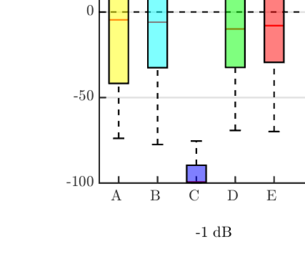
Figure 1: $T_{\textrm{60}}$ estimation error for Ambient noise for computation methods A to E for low ($-1\text{\,}\mathrm{dB}$), medium ($12\text{\,}\mathrm{dB}$) and high ($18\text{\,}\mathrm{dB}$) SNRs

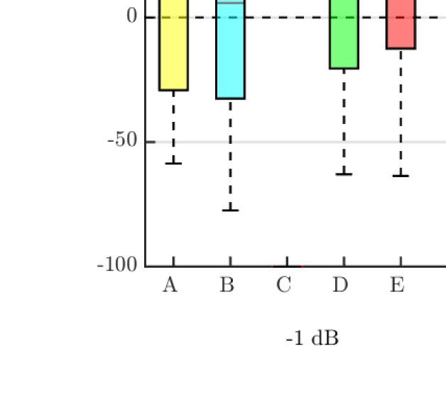
Figure 2: $T_{\textrm{60}}$ estimation error for Fan noise for computation methods A to E for low ($-1\text{\,}\mathrm{dB}$), medium ($12\text{\,}\mathrm{dB}$) and high ($18\text{\,}\mathrm{dB}$) SNRs

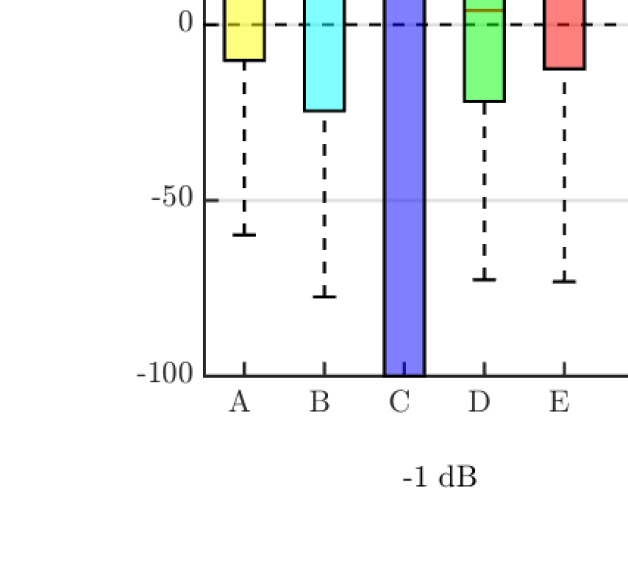
Figure 3: $T_{\textrm{60}}$ estimation error for Babble noise for computation methods A to E for low ($-1\text{\,}\mathrm{dB}$), medium ($12\text{\,}\mathrm{dB}$) and high ($18\text{\,}\mathrm{dB}$) SNRs

On each box, the central mark is the median, the edges of the box are the $25$th and $75$th percentiles, the whiskers extend to the most extreme data points not considered outliers. Outliers are not shown.

The results show that method C does not cope well in noise confirming the results of [8]. This is because as the noise level increases, it causes the average gradient in each frame of STFT time-frequency bins to approach zero resulting in very small NSV. This is the same effect as having a very long $T_{\textrm{60}}$. The algorithm will in general therefore tend to overestimate, however, the relationship between the NSV and the $T_{\textrm{60}}$ is based on a trained mapping function which can result in a negative value of $T_{\textrm{60}}$, and in such circumstances the algorithm returns an estimate of $0\text{\,}\mathrm{s}$.

In babble noise, the end-point decays of the babble will have the same $T_{\textrm{60}}$ as the speech. Under these circumstances method C gives a better estimate.

The remaining methods give similar levels of performance with fan noise being the most challenging environment in which to estimate at low SNRs for all algorithms.

Table 1 shows the RTF for each algorithm computed by dividing the total CPU time used to process all $4500$ noisy reverberant speech files in the ACE Evaluation dataset by the combined length of all the noisy reverberant speech files.

Table 1: Comparison of RTF

A [6] B [7] C [5] D [4] E [4] $0.457$ $0.131$ $0.0219$ $0.0166$ $0.0153$

This results in a much lower RTF in the Matlab implementation. The perceptually motivated averaging using Mel-spaced frequency bands in D and E gives a further reduction in RTF.

5 Conclusion

The ACE Challenge has provided an opportunity to evaluate the author’s algorithm on real recordings of AIRs and noise in contrast to the previously reported performance which was on simulated data. Also, the speech in the ACE corpus is free-running and less uniform than the TIMIT database used in [4], and so is representative of conversational speech rather than read speech. The estimation performance compares well with existing methods, and has a low RTF making it suitable for real-time applications.

References

- [1] ISO, ISO-3382 Acoustics - Measurement of the Reverberation Time of Rooms with Reference to Other Acoustical Parameters, Intl. Org. for Standardization (ISO) Recommendation ISO-3382, May 2009.
- [2] S. Mosayyebpour, H. Sheikhzadeh, T. Gulliver, and M. Esmaeili, “Single-microphone LP residual skewness-based inverse filtering of the room impulse response,” IEEE Trans. Audio, Speech, Lang. Process., vol. 20, no. 5, pp. 1617–1632, July 2012.
- [3] P. A. Naylor and N. D. Gaubitch, “Acoustic signal processing in noise: It’s not getting any quieter,” in Proc. Intl. Workshop Acoust. Signal Enhancement (IWAENC), Aachen, Germany, 2012, pp. 1–6.
- [4] J. Eaton, N. D. Gaubitch, and P. A. Naylor, “Noise-robust reverberation time estimation using spectral decay distributions with reduced computational cost,” in Proc. IEEE Intl. Conf. on Acoustics, Speech and Signal Processing (ICASSP), Vancouver, Canada, May 2013, pp. 161–165.
- [5] J. Y. C. Wen, E. A. P. Habets, and P. A. Naylor, “Blind estimation of reverberation time based on the distribution of signal decay rates,” in Proc. IEEE Intl. Conf. on Acoustics, Speech and Signal Processing (ICASSP), Las Vegas, USA, Apr. 2008, pp. 329–332.
- [6] T. H. Falk, C. Zheng, and W.-Y. Chan, “A non-intrusive quality and intelligibility measure of reverberant and dereverberated speech,” IEEE Trans. Audio, Speech, Lang. Process., vol. 18, no. 7, pp. 1766–1774, Sept. 2010.
- [7] H. W. Löllmann, E. Yilmaz, M. Jeub, and P. Vary, “An improved algorithm for blind reverberation time estimation,” in Proc. Intl. Workshop Acoust. Echo and Noise Control (IWAENC), Tel-Aviv, Israel, Aug. 2010, pp. 1–4.
- [8] N. D. Gaubitch, H. W. Löllmann, M. Jeub, T. H. Falk, P. A. Naylor, P. Vary, and M. Brookes, “Performance comparison of algorithms for blind reverberation time estimation from speech,” in Proc. Intl. Workshop Acoust. Signal Enhancement (IWAENC), Aachen, Germany, Sept. 2012, pp. 1–4.
- [9] E. H. Moore, “On the reciprocal of the general algebraic matrix,” Bulletin of the American Mathematical Society, vol. 26, no. 9, pp. 394–395, 1920.
- [10] J. Eaton, N. D. Gaubitch, A. H. Moore, and P. A. Naylor, “The ACE challenge - corpus description and performance evaluation,” in Proc. IEEE Workshop on Applications of Signal Processing to Audio and Acoustics (WASPAA), New Paltz, NY, USA, 2015.
- [11] D. M. Brookes, “VOICEBOX: A speech processing toolbox for MATLAB,” http://www.ee.ic.ac.uk/hp/staff/dmb/voicebox/voicebox.html, 1997–2015.