Formulation of discontinuous Galerkin methods for relativistic astrophysics

Abstract

The DG algorithm is a powerful method for solving pdes, especially for evolution equations in conservation form. Since the algorithm involves integration over volume elements, it is not immediately obvious that it will generalize easily to arbitrary time-dependent curved spacetimes. We show how to formulate the algorithm in such spacetimes for applications in relativistic astrophysics. We also show how to formulate the algorithm for equations in non-conservative form, such as Einstein’s field equations themselves. We find two computationally distinct formulations in both cases, one of which has seldom been used before for flat space in curvilinear coordinates but which may be more efficient. We also give a new derivation of the ALE algorithm (Arbitrary Lagrangian-Eulerian) using 4-vector methods that is much simpler than the usual derivation and explains why the method preserves the conservation form of the equations. The various formulations are explored with some simple numerical experiments that also explore the effect of the metric identities on the results.

1 Introduction

In relativistic astrophysics, simulations involving hydrodynamics or magnetohydrodynamics or similar physics are most often carried out using finite-volume methods. Two major challenges of such simulations are accuracy and computational efficiency. Many important problems cannot be solved to the required accuracy using currently available hardware resources. Accuracy can be improved only by increasing numerical resolution. If parts of the solution are smooth so that one might want to take advantage of high-order methods to improve the accuracy, current methods eventually run into problems. High-order finite-volume methods couple together more cells and require more communication between cells. Ultimately, when the number of cells and processors gets large enough, the communication time begins to limit the computation and the code no longer scales with the number of processors. Moreover, astrophysical applications often involve multiphysics (fluids, magnetic fields, neutrinos, electromagnetic radiation, relativistic gravity). With current formulations, each new type of physics often requires its own computational treatment, making coupling of the physics difficult. As one looks ahead to the arrival of exascale computing, it seems that we should look to the development of algorithms that can take advantage of these very large machines properly for astrophysics.

In the last decade, discontinuous Galerkin (DG) methods have emerged as the leading contender to achieve all the goals of a general purpose simulation code, particularly for equations in conservation form: high order accuracy in smooth regions, robustness for shocks and other discontinuities, scalability to very large machines, accurate handling of irregular boundaries, adaptivity, and so on. Many applications of DG in terrestrial fluid dynamics have appeared. However, applications in relativity and astrophysics have so far been mainly exploratory[1, 2, 3, 4, 5, 6, 7, 8, 9, 10] and confined to simple problems.

The goal of this paper is to formulate the DG method for arbitrary 3-dimensional problems involving general relativistic gravitation. At first sight, this sounds tricky: the basic DG algorithm involves integrating the pdes over space and using Gauss’s Theorem to turn integrals of divergences into surface integrals. In general relativity, spacetime is curved and coordinates are arbitrary and not necessarily simply related to physical measurements by an observer. So should integrations be performed over coordinate volume or proper volume? What are the corresponding normal vectors that enter into the interface flux prescriptions? How should Einstein’s equations, which are not typically in conservation form, be handled? Is the weak form or the strong form of the equations better? How do the so-called metric identities affect the formulation? We give answers to these questions. In particular, we find that the final formulation is very close to that already developed for Euclidean space in curvilinear coordinates. Moreover, the covariant approach adopted in this paper gives new insights into the standard curvilinear coordinate treatment. Not only are derivations much simpler, but alternative formulations that may be more efficient computationally are found.

Here we summarize the key results in this paper.

• Despite the curvature of spacetime, the DG algorithm can easily be formulated in general relativity. In fact, the formulation is analogous to that for curvilinear coordinates in flat spacetime.

• In the general case, there are two distinct strong formulations for conservation laws. For the tensor-product basis functions used in this paper, the corresponding weak formulations are both equivalent to one of the strong formulations.

• Only one of the formulations has been widely used for flat space in curvilinear coordinates. In numerical experiments, the other appears to be somewhat more efficient and should be further investigated.

• Similarly, there are two inequivalent formulations for hyperbolic equations in non-conservation form. These formulations are important for solving Einstein’s equations.

• Time-dependent mappings (Arbitrary Lagrangian-Eulerian (ALE) methods and the dual-frame approach[11] that has proved useful for black hole simulations) are easily implemented in the relativistic treatment.

• We give streamlined derivations of the so-called metric identities, the geometric conservation law, and the ALE method for moving grids. The derivation of the ALE method is novel and uses general covariance to get the result in a few lines. In addition, the reason that the ALE method preserves the conservation form of the equations is explained.

• Satisfying the metric identities discretely is often claimed to be a necessary condition for “free-stream preservation,” or the requirement that a uniform flow remain uniform for all time. We show that in fact this statement is true for only one of the computational formulations of the DG algorithm and not the other.

• We clarify how normal vectors should be normalized. The normal vector that the boundary flux vector is projected along does not need to be the unit normal—the normalization factor cancels out of the algorithm.

A covariant treatment of DG in general relativity has previously been given by Radice and Rezzolla[4]. This paper covers many aspects that were not covered by them.

2 DG for equations in conservation form

2.1 Form of the equations

In a general time-dependent curved spacetime, a conservation law can be written in terms of a 4-divergence:

$$\nabla_{\mu}F^{\mu}=0,$$ (2.1)

where $\nabla_{\mu}$ denotes the covariant derivative. Here and throughout, repeated indices are summed over. Greek indices $\mu,\nu,\ldots$ range from 0 to 3, while Latin indices $a,b,\ldots$ will be purely spatial, ranging from 1 to 3. We choose units with the speed of light $c=1$, so that $x^{0}=t$. We will often denote $F^{0}$ by $u$, a quantity like density that is conserved. The spatial flux vector $F^{a}$ is generally a function of $u$. In practice, rather than a single conservation law like (2.1), one deals with a system of conservation laws. In this case, $u$ is a vector of conserved quantities and $F^{a}$ is a vector of flux vectors. For example, $u$ and $F^{a}$ are vectors of length 5 for hydrodynamics. In this paper, we will typically not need to deal with the various separate equations in a system of conservation laws. Accordingly, we will write $u$ and $F^{a}$ whether we are dealing with one equation or a system. All the derivations go through independently on each equation in a system.

It will be convenient to generalize (2.1) to allow a source term $s$ on the right-hand side. Such a source term arises, for example, when one considers conservation of energy and momentum in a general curved (or curvilinear) metric. The divergence of the energy-momentum tensor gives an extra term that cannot be included as the pure divergence of a flux vector. However, the extra term depends only on $u$ and not on its derivatives. This is the key requirement that we place on the source term in the subsequent treatment.

The metric in a general spacetime can be written in the standard $3+1$ form

$$ds^{2}=g_{\mu\nu}dx^{\mu}dx^{\nu}=-\alpha^{2}dt^{2}+\gamma_{ab}(dx^{a}+\beta^{a}dt)(dx^{b}+\beta^{b}dt),$$ (2.2)

where $\alpha$ is called the lapse function, $\beta^{a}$ the shift vector, and $\gamma_{ab}$ is the spatial metric on $t=\text{constant}$ slices. (For more on the $3+1$ decomposition, see, e.g., [12] or [13].) In flat spacetime (no relativistic gravitational field), we can set $\alpha=1$, $\beta=0$. In Cartesian coordinates, $\gamma_{ab}=\delta_{ab}$, the Euclidean 3-metric.

Now using a standard identity for the covariant divergence (see, e.g., Problem 7.7(g) in [14]), the conservation equation (2.1) with source term can be written

$$\frac{1}{\sqrt{-g}}\partial_{t}(\sqrt{-g}u)+\frac{1}{\sqrt{-g}}\partial_{a}(\sqrt{-g}F^{a})=s,$$ (2.3)

where $g$ is the determinant of the 4-metric $g_{\mu\nu}$. It is easy to show from (2.2) that $\sqrt{-g}=\alpha\sqrt{\gamma}$, where $\gamma$ is the determinant of $\gamma_{ab}$. So Eq. (2.3) becomes

$$\frac{1}{\sqrt{\gamma}}\partial_{t}(\sqrt{\gamma}u)+\frac{1}{\sqrt{\gamma}}\partial_{a}(\sqrt{\gamma}F^{a})=s.$$ (2.4)

Here we have absorbed the factor of $\alpha$ in the definitions of $u$, $F^{a}$, and $s$, which is standard practice in computational relativity. Multiplying Eq. (2.4) through by $\sqrt{\gamma}$ gives

$$\partial_{t}(\sqrt{\gamma}u)+\partial_{a}(\sqrt{\gamma}F^{a})=\sqrt{\gamma}s,$$ (2.5)

which suggests that $\sqrt{\gamma}u$, $\sqrt{\gamma}F^{a}$, and $\sqrt{\gamma}s$ might be convenient variables to use in a code.

Note that Eq. (2.4) or (2.5) is formally the same as a conservation law in flat space written in curvilinear coordinates. In that case the metric is simply the Euclidean metric transformed to the curvilinear coordinates, whereas here we consider the more general case where the metric might be the solution of Einstein’s equations of general relativity in an arbitrary coordinate system.

2.2 The DG algorithm in curved spacetime

As we will see, the DG algorithm is remarkably similar in flat and curved spacetimes. However, at key points there are important details that need to be correctly implemented.

The algorithm starts by dividing the spatial domain into subdomains, often called cells or elements. Each element is a mapping of a reference element (triangle or square in 2-d, tetrahedron or cube in 3-d). The mapped elements can have straight or curved sides. (Here “straight” means having two constant spatial coordinates.) In each element, the quantities $u$, $F^{a}$, $s$, etc. (or equivalently $\sqrt{\gamma}u$, $\sqrt{\gamma}F^{a}$, $\sqrt{\gamma}s$) are each expanded in term of a set of basis functions, typically polynomials:

$$u(\mbox{$\mathbf{x}$})=\sum_{i}u_{i}\phi_{i}(\mbox{$\mathbf{x}$}).$$ (2.6)

Analogous to spectral collocation methods, we will work with a so-called nodal expansion, where Eq. (2.6) is an interpolation:

$$u(\mbox{$\mathbf{x}$}_{i})=u_{i},\qquad i=0,\ldots,N$$ (2.7)

for some choice of nodes (grid points) $\mbox{$\mathbf{x}$}_{i}$. This implies that $\phi_{i}(\mbox{$\mathbf{x}$}_{j})=\delta_{ij}$. Such basis functions are called cardinal functions. For polynomial basis functions, they will be simply Lagrange interpolating polynomials.

Get the DG equations by integrating Eq. (2.4) in each element with test functions that are the same as the basis functions:

$$\int\left[\partial_{t}\left(\sqrt{\gamma}u\right)+\partial_{a}\left(\sqrt{\gamma}F^{a}\right)-\sqrt{\gamma}s\right]\phi_{i}(\mbox{$\mathbf{x}$})\,d^{3}x=0.$$ (2.8)

Here we have integrated with respect to proper volume $\sqrt{\gamma}d^{3}x$, where $d^{3}x$ is the coordinate volume element $dx\,dy\,dz$. Had we started with the form (2.5), then we would have integrated with respect to coordinate volume instead. The choice is designed to allow Gauss’s Theorem to be invoked in a simple way, as we now show.

Transform the spatial derivative term by integrating by parts:

$$\int\partial_{a}\left(\sqrt{\gamma}F^{a}\right)\phi_{i}(\mbox{$\mathbf{x}$})\,d^{3}x =\int\partial_{a}\left(\sqrt{\gamma}F^{a}\phi_{i}(\mbox{$\mathbf{x}$})\right)\,d^{3}x-\int\sqrt{\gamma}F^{a}\partial_{a}\phi_{i}(\mbox{$\mathbf{x}$})\,d^{3}x$$

$$=\oint F^{a}n_{a}\phi_{i}\,d^{2}\Sigma-\int\sqrt{\gamma}F^{a}\partial_{a}\phi_{i}(\mbox{$\mathbf{x}$})\,d^{3}x.$$ (2.9)

Here $d^{2}\Sigma$ is the proper surface element of the cell and $n_{a}$ is the unit outward normal (see A for more on Gauss’s Theorem and normal vectors.)

With a formulation like (2.9) in each element, there is no connection between the elements. The heart of the DG method is to replace $F^{a}$ in the surface term by the numerical flux $F^{a*}$, a function of the fluxes on both sides of the interface:

$$\int\partial_{a}\left(\sqrt{\gamma}F^{a}\right)\phi_{i}(\mbox{$\mathbf{x}$})\,d^{3}x\to\oint F^{a*}n_{a}\phi_{i}\,d^{2}\Sigma-\int\sqrt{\gamma}F^{a}\partial_{a}\phi_{i}(\mbox{$\mathbf{x}$})\,d^{3}x.$$ (2.10)

This gives the weak form of the equations (no derivatives of $F^{a}$). To get the strong form, undo the integration by parts on the right-hand side of Eq. (2.10):

$$\int\partial_{a}\left(\sqrt{\gamma}F^{a}\right)\phi_{i}(\mbox{$\mathbf{x}$})\,d^{3}x\to\oint(F^{a*}-F^{a})n_{a}\phi_{i}\,d^{2}\Sigma+\int\partial_{a}\left(\sqrt{\gamma}F^{a}\right)\phi_{i}(\mbox{$\mathbf{x}$})\,d^{3}x.$$ (2.11)

So one question we will have to answer is: Should we use the weak form (2.10) or the strong form (2.11)? We will return to this question in §4.3.

2.2.1 The mass matrix

Evaluation of Eq. (2.8) now follows standard lines as in flat spacetime. The first term gives the mass matrix:

$$\int\partial_{t}\left(\sqrt{\gamma}u\right)\phi_{i}(\mbox{$\mathbf{x}$})\,d^{3}x =\frac{d}{dt}\sum_{j}\left(\sqrt{\gamma}u\right)_{j}\int\phi_{j}(\mbox{$\mathbf{x}$})\phi_{i}(\mbox{$\mathbf{x}$})\,d^{3}x$$

$$=\mbox{$\mathbf{M}$}\cdot\frac{d\left(\sqrt{\mbox{$\boldsymbol{\gamma}$}}\mbox{$\mathbf{u}$}\right)}{dt}\Big{|}_{i},$$ (2.12)

where the mass matrix $\mathbf{M}$ has components

$$M_{ij}=\int\phi_{i}(\mbox{$\mathbf{x}$})\phi_{j}(\mbox{$\mathbf{x}$})\,d^{3}x$$ (2.13)

and the dot in Eq. (2.12) denotes matrix-vector multiplication.

Note that a product like $\sqrt{\gamma}u$ is expanded using the product of the function values at the grid points for each factor:

$$\sqrt{\gamma}u=\sum_{j}\sqrt{\gamma_{j}}u_{j}\phi_{j}(\mbox{$\mathbf{x}$}).$$ (2.14)

This is not exact in general unless $\gamma$ is constant, and will introduce aliasing that may have to be dealt with by filtering. We will handle all products in this way. The notation $\sqrt{\mbox{$\boldsymbol{\gamma}$}}\mbox{$\mathbf{u}$}$ is used to denote the vector whose elements are $\sqrt{\gamma_{j}}u_{j}$.

Similarly, the last term in Eq. (2.8) gives

$$-\int\left(\sqrt{\gamma}s\right)\phi_{i}(\mbox{$\mathbf{x}$})\,d^{3}x=-\mbox{$\mathbf{M}$}\cdot\left(\sqrt{\mbox{$\boldsymbol{\gamma}$}}\mbox{$\mathbf{s}$}\right)|_{i}.$$ (2.15)

2.2.2 The volume derivative term

For the strong form, the derivative term in Eq. (2.8) gives the boundary and volume terms as in Eq. (2.11). Note that all spatial derivatives can be rewritten using the derivative matrices defined by

$$D^{(a)}_{ij}=\partial_{a}\phi_{j}(\mbox{$\mathbf{x}$}_{i}).$$ (2.16)

Explicitly, for any quantity $f(\mbox{$\mathbf{x}$})$ we have

$$f(\mbox{$\mathbf{x}$})=\sum_{k}f_{k}\phi_{k}(\mbox{$\mathbf{x}$})\quad\Rightarrow\quad\partial_{a}f(\mbox{$\mathbf{x}$})=\sum_{k}f_{k}\partial_{a}\phi_{k}(\mbox{$\mathbf{x}$})\quad\Rightarrow\quad\partial_{a}f(\mbox{$\mathbf{x}$})|_{j}=\sum_{k}D^{(a)}_{jk}f_{k}.$$ (2.17)

Applying this to the derivative in Eq. (2.11) gives

$$\partial_{a}\left(\sqrt{\gamma}F^{a}\right)=\sum_{j}\left[\partial_{a}\left(\sqrt{\gamma}F^{a}\right)\right]_{j}\phi_{j}(\mbox{$\mathbf{x}$})=\sum_{jk}D^{(a)}_{jk}\left(\sqrt{\gamma}F^{a}\right)_{k}\phi_{j}(\mbox{$\mathbf{x}$}).$$ (2.18)

Thus the volume term becomes

$$\int\partial_{a}\left(\sqrt{\gamma}F^{a}\right)\phi_{i}(\mbox{$\mathbf{x}$})\,d^{3}x =\sum_{jk}D^{(a)}_{jk}\left(\sqrt{\gamma}F^{a}\right)_{k}\int\phi_{j}(\mbox{$\mathbf{x}$})\phi_{i}(\mbox{$\mathbf{x}$})\,d^{3}x$$

$$=\sum_{jk}M_{ij}D^{(a)}_{jk}\left(\sqrt{\gamma}F^{a}\right)_{k}$$

$$=\mbox{$\mathbf{M}$}\cdot\mbox{$\mathbf{D}$}^{(a)}\cdot\left(\sqrt{\mbox{$\boldsymbol{\gamma}$}}\,\mbox{$\mathbf{F}$}^{a}\right)\big{|}_{.}$$ (2.19)

2.2.3 The boundary flux

For the boundary surface term, define

$$F\equiv(F^{a*}-F^{a})n_{a}.$$ (2.20)

For smooth problems the numerical flux is generally evaluated by upwinding. For non-smooth solutions, the flux prescription typically enforces the Rankine-Hugoniot relations in some way. So let’s assume we have some prescription for $F$ on the boundary and that this has been computed as an expansion in terms of the basis functions. Then

$$\oint F\phi_{i}\,d^{2}\Sigma=\sum_{j}F_{j}\oint\phi_{j}(\mbox{$\mathbf{x}$})\phi_{i}(\mbox{$\mathbf{x}$})\,\ d^{2}\Sigma.$$ (2.21)

Write this as

$$\oint F\phi_{i}\,d^{2}\Sigma=\sum_{\rm surfaces}\mbox{$\mathbf{M}$}^{(2)}\cdot\mbox{$\mathbf{F}$}\big{|}_{i},$$ (2.22)

where the surface mass matrix on each piece of the boundary surface is defined as

$$M^{(2)}_{ij}=\int\limits_{\rm surface}\phi_{i}(\mbox{$\mathbf{x}$})\phi_{j}(\mbox{$\mathbf{x}$})\,d^{2}\Sigma.$$ (2.23)

2.3 The equations of motion

Now put all the pieces together: Substitute Eqs. (2.12), (2.15), (2.19) and (2.22) in Eq. (2.8) and multiply through by $\mbox{$\mathbf{M}$}^{-1}$ to get

$$\frac{d\left(\sqrt{\mbox{$\boldsymbol{\gamma}$}}\mbox{$\mathbf{u}$}\right)}{dt}+\mbox{$\mathbf{D}$}^{(a)}\cdot\left(\sqrt{\mbox{$\boldsymbol{\gamma}$}}\,\mbox{$\mathbf{F}$}^{a}\right)-\left(\sqrt{\mbox{$\boldsymbol{\gamma}$}}\mbox{$\mathbf{s}$}\right)=-\mbox{$\mathbf{M}$}^{-1}\cdot\sum_{\rm surfaces}\mbox{$\mathbf{M}$}^{(2)}\cdot\mbox{$\mathbf{F}$}.$$ (2.24)

This is the form that is integrated with a suitable time stepper. We see that the algorithm resembles the method of lines in finite-volume methods.

3 Evaluation of Integrals

Evaluate the various integrals by mapping them to the reference element and then doing a Gaussian quadrature. Let the mapping be some time-independent function

$$\mbox{$\mathbf{x}$}=\mbox{$\mathbf{x}$}(\mathbf{\bar{x}})$$ (3.1)

with Jacobian matrix

$$\mbox{$\mathbf{J}$}=\frac{\partial x^{a}}{\partial x^{\bar{a}}}$$ (3.2)

and Jacobian

$$J=\det\mbox{$\mathbf{J}$}.$$ (3.3)

Here the barred coordinates are some standard coordinates covering the reference element, which we will sometimes also denote as

$$(x^{\bar{1}},x^{\bar{2}},x^{\bar{3}})=(a^{1},a^{2},a^{3}).$$ (3.4)

Note the standard relativist’s convention of placing the bar on the index: $x^{\bar{a}}$ in (3.2) rather than $\bar{x}^{a}$, which facilitates working with tensor indices.

We will take the reference element to be a cube with extents $[-1,1]$ in each direction. The boundaries in most typical astrophysics problems are sufficiently simple that we don’t need the flexibility of grids composed of triangles or tetrahedra. Even for binary black hole simulations, where the centers of each black hole are excised from the computational domain, we only need a domain bounded by a large sphere at infinity with two interior holes removed. Such a domain can easily be covered with elements that are mapped cubes.

Using cubes allows a big simplification in the algorithm: We can take the basis functions to be a tensor product of 1-d basis functions $\ell_{i}$ on the reference element:

$$\phi_{i}(\mbox{$\mathbf{x}$})\to\phi_{ijk}(\mbox{$\mathbf{x}$})=\ell_{i}\big{(}x^{\bar{1}}\big{)}\ell_{j}\big{(}x^{\bar{2}}\big{)}\ell_{k}\big{(}x^{\bar{3}}\big{)}.$$ (3.5)

Since the Gaussian quadrature along each dimension is being carried out with a weight function of unity, it should be a Gauss-Legendre quadrature, with nodes $\bar{x}_{i}$ corresponding to roots of an appropriate Legendre polynomial. A further simplification follows if we assume that these quadrature points are chosen to be the same as the interpolation points. The combination of tensor product basis functions and quadrature points the same as interpolation points gives a very simple form of the equations that resembles multipenalty collocation. It also implies that the basis functions are the Lagrange interpolating polynomials corresponding to Legendre polynomials:

$$\ell_{i}(\bar{x})=\prod_{\begin{subarray}{c}j=0\\ j\neq i\end{subarray}}^{N}\frac{\bar{x}-\bar{x}_{j}}{\bar{x}_{i}-\bar{x}_{j}}.$$ (3.6)

Note that we can have different numbers of points along each dimension in (3.5), which will lead to different values for the quadrature points $\bar{x}_{i}$ and weights $w_{i}$ along each dimension. We will not clutter the notation to make this distinction. Also, we now have to give up the nice matrix notation we used above, since each matrix index becomes a triple like $(ijk)$.

3.1 The mass matrix

Equation (2.13) for the mass matrix becomes

$$M_{ij}\to M_{(ijk)(lmn)} =\int\phi_{ijk}(\mbox{$\mathbf{x}$})\phi_{lmn}(\mbox{$\mathbf{x}$})\,d^{3}x$$

$$=\int\ell_{i}\big{(}x^{\bar{1}}\big{)}\ell_{j}\big{(}x^{\bar{2}}\big{)}\ell_{k}\big{(}x^{\bar{3}}\big{)}\ell_{l}\big{(}x^{\bar{1}}\big{)}\ell_{m}\big{(}x^{\bar{2}}\big{)}\ell_{n}\big{(}x^{\bar{3}}\big{)}J(\mathbf{\bar{x}})\,d^{3}\bar{x}$$

$$=\sum_{pqr}\ell_{i}\big{(}x^{\bar{1}}_{p}\big{)}\ell_{l}\big{(}x^{\bar{1}}_{p}\big{)}w_{p}\ell_{j}\big{(}x^{\bar{2}}_{q}\big{)}\ell_{m}\big{(}x^{\bar{2}}_{q}\big{)}w_{q}\ell_{k}\big{(}x^{\bar{3}}_{r}\big{)}\ell_{n}\big{(}x^{\bar{3}}_{r}\big{)}w_{r}J\big{(}x^{\bar{1}}_{p},x^{\bar{2}}_{q},x^{\bar{3}}_{r}\big{)}$$

$$=\sum_{pqr}\delta_{ip}\delta_{lp}w_{p}\delta_{jq}\delta_{mq}w_{q}\delta_{kr}\delta_{nr}w_{r}J_{pqr}$$

$$=\delta_{il}\delta_{jm}\delta_{kn}w_{i}w_{j}w_{k}J_{ijk}.$$ (3.7)

Here we have used the equality of quadrature and interpolation points to set quantities like $\ell_{i}\big{(}x^{\bar{1}}_{p}\big{)}$ equal to $\delta_{ip}$. The resulting mass matrix is diagonal in each dimension.

The “matrix” multiplication of the expression (3.7) by a term like $d(\sqrt{\gamma}u)/dt|_{lmn}$ gives

$$w_{i}w_{j}w_{k}J_{ijk}\frac{d(\sqrt{\gamma}u)_{ijk}}{dt},$$ (3.8)

and a similar term for Eq. (2.15).

3.2 The volume derivative term

Corresponding to the manipulations in Eq. (2.17) we have

$$f(\mbox{$\mathbf{x}$})=\sum_{ijk}f_{ijk}\phi_{ijk}(\mbox{$\mathbf{x}$})\quad \Rightarrow\quad\partial_{a}f(\mbox{$\mathbf{x}$})=\sum_{ijk}f_{ijk}\partial_{a}\phi_{ijk}(\mbox{$\mathbf{x}$})$$

$$\Rightarrow\quad\partial_{a}f(\mbox{$\mathbf{x}$})|_{lmn}=\sum_{ijk}f_{ijk}\partial_{a}\phi_{ijk}(\mbox{$\mathbf{x}$}_{lmn}).$$ (3.9)

Mapping to the reference element gives

$$\partial_{a}\phi_{ijk}(\mbox{$\mathbf{x}$}_{lmn}) =\frac{\partial x^{\bar{a}}}{\partial x^{a}}\partial_{\bar{a}}\phi_{ijk}(\mathbf{\bar{x}})\big{|}_{lmn}$$

$$=\frac{\partial x^{\bar{a}}}{\partial x^{a}}\partial_{\bar{a}}\ell_{i}\big{(}x^{\bar{1}}\big{)}\ell_{j}\big{(}x^{\bar{2}}\big{)}\ell_{k}\big{(}x^{\bar{3}}\big{)}\big{|}_{lmn}$$

$$=\frac{\partial x^{\bar{1}}}{\partial x^{a}}D_{li}^{\bar{1}}\delta_{jm}\delta_{kn}+\frac{\partial x^{\bar{2}}}{\partial x^{a}}D_{mj}^{\bar{2}}\delta_{il}\delta_{kn}+\frac{\partial x^{\bar{3}}}{\partial x^{a}}D_{nk}^{\bar{3}}\delta_{il}\delta_{jm},$$ (3.10)

where

$$D_{li}^{\bar{1}}=\partial_{\bar{1}}\ell_{i}\big{(}x^{\bar{1}}\big{)}\big{|}_{l}$$ (3.11)

is the derivative matrix for $x^{\bar{1}}$, and similarly for the 2- and 3-coordinates. Substituting Eq. (3.10) in Eq. (3.9) gives

$$\partial_{a}f(\mbox{$\mathbf{x}$})|_{lmn}=\frac{\partial x^{\bar{1}}}{\partial x^{a}}\Big{|}_{lmn}\sum_{i}D_{li}^{\bar{1}}f_{imn}+\frac{\partial x^{\bar{2}}}{\partial x^{a}}\Big{|}_{lmn}\sum_{j}D_{mj}^{\bar{2}}f_{ljn}+\frac{\partial x^{\bar{3}}}{\partial x^{a}}\Big{|}_{lmn}\sum_{k}D_{nk}^{\bar{3}}f_{lmk}.$$ (3.12)

So analogously to Eq. (2.18) we get

$$\partial_{a}\left(\sqrt{\gamma}F^{a}\right)=\sum_{lmn}\left[\partial_{a}\left(\sqrt{\gamma}F^{a}\right)\right]_{lmn}\phi_{lmn}(\mbox{$\mathbf{x}$}),$$ (3.13)

where $[\partial_{a}\left(\sqrt{\gamma}F^{a}\right)]_{lmn}$ is given by the analog of Eq. (3.12). Thus the volume term (2.19) gives

$$\int\partial_{a}\left(\sqrt{\gamma}F^{a}\right)\phi_{i}(\mbox{$\mathbf{x}$})\,d^{3}x =\sum_{lmn}\left[\partial_{a}\left(\sqrt{\gamma}F^{a}\right)\right]_{lmn}\int\phi_{lmn}(\mbox{$\mathbf{x}$})\phi_{ijk}(\mbox{$\mathbf{x}$})\,d^{3}x$$

$$=\sum_{lmn}\left[\partial_{a}\left(\sqrt{\gamma}F^{a}\right)\right]_{lmn}M_{(ijk)(lmn)}$$

$$=\left[\partial_{a}\left(\sqrt{\gamma}F^{a}\right)\right]_{ijk}w_{i}w_{j}w_{k}J_{ijk},$$ (3.14)

where we have used Eq. (3.7) in the last line.

3.3 The boundary flux

Let’s consider the flux through the surface corresponding to $a^{3}=x^{\bar{3}}=1$ on the reference element. Evaluating Eq. (2.21) by transforming to the reference element gives

$$\int F\phi_{ijk}(\mbox{$\mathbf{x}$})\,d^{2}\Sigma=\sum_{lmn}F_{lmn}\int\limits_{a^{3}=1}\ell_{l}\big{(}x^{\bar{1}}\big{)}\ell_{m}\big{(}x^{\bar{2}}\big{)}\ell_{n}\big{(}x^{\bar{3}}\big{)}\ell_{i}\big{(}x^{\bar{1}}\big{)}\ell_{j}\big{(}x^{\bar{2}}\big{)}\ell_{k}\big{(}x^{\bar{3}}\big{)}\sqrt{{}^{(2)}\gamma\big{(}x^{\bar{1}},x^{\bar{2}}\big{)}}\,dx^{\bar{1}}\,dx^{\bar{2}}.$$ (3.15)

Here ${}^{(2)}\gamma$ is the determinant of the 2-dimensional metric induced on the surface by $\gamma_{ij}$.

Assume the quadrature uses Gauss-Lobatto points. Then $\ell_{k}\big{(}x^{\bar{3}}\big{)}=\delta_{kN}$, where $N$ is the last grid point. Equation (3.15) becomes

$$\int F\phi_{ijk}(\mbox{$\mathbf{x}$})\,d^{2}\Sigma =\sum_{lmn,pq}F_{lmn}\sqrt{{}^{(2)}\gamma_{pq}}\,\delta_{lp}\delta_{mq}\delta_{nN}\delta_{ip}\delta_{jq}\delta_{kN}w_{p}w_{q}$$

$$=F_{ijN}\sqrt{{}^{(2)}\gamma_{ij}}\,w_{i}w_{j}\delta_{kN}.$$ (3.16)

Integrating over the surface $a^{3}=-1$ gives a similar term with a minus sign and $N$ replaced by the index 0, corresponding to the first grid point in the interval. The contributions from the other 4 sides of the cube are similar.

3.4 The equations of motion — strong form

Putting together Eqs. (3.8), (3.14), (3.12) and (3.16), and dividing through by $w_{i}w_{j}w_{k}J_{ijk}$, we get

$$\frac{d(\sqrt{\gamma}u)_{ijk}}{dt} +\Big{[}\frac{\partial x^{\bar{1}}}{\partial x^{a}}\Big{|}_{ijk}\sum_{l}D_{il}^{\bar{1}}\left(\sqrt{\gamma}F^{a}\right)_{ljk}+\frac{\partial x^{\bar{2}}}{\partial x^{a}}\Big{|}_{ijk}\sum_{m}D_{jm}^{\bar{2}}\left(\sqrt{\gamma}F^{a}\right)_{imk}$$

$$\quad+\frac{\partial x^{\bar{3}}}{\partial x^{a}}\Big{|}_{ijk}\sum_{n}D_{kn}^{\bar{3}}\left(\sqrt{\gamma}F^{a}\right)_{ijn}\Big{]}-(\sqrt{\gamma}s)_{ijk}$$

$$=-\frac{1}{w_{N}}F_{ijN}\frac{\sqrt{{}^{(2)}\gamma_{ij}}}{J_{ijN}}\delta_{kN}+\frac{1}{w_{0}}F_{ij0}\frac{\sqrt{{}^{(2)}\gamma_{ij}}}{J_{ij0}}\delta_{k0}-\frac{1}{w_{N}}F_{Njk}\frac{\sqrt{{}^{(2)}\gamma_{jk}}}{J_{Njk}}\delta_{iN}$$

$$\quad+\frac{1}{w_{0}}F_{0jk}\frac{\sqrt{{}^{(2)}\gamma_{jk}}}{J_{0jk}}\delta_{i0}-\frac{1}{w_{N}}F_{iNk}\frac{\sqrt{{}^{(2)}\gamma_{ik}}}{J_{iNk}}\delta_{jN}+\frac{1}{w_{0}}F_{i0k}\frac{\sqrt{{}^{(2)}\gamma_{ik}}}{J_{i0k}}\delta_{j0}.$$ (3.17)

The relatively simple form for the boundary flux terms in Eq. (3.17) occurs because of the 1-d Gauss-Lobatto quadratures using the interpolation points.

Note that the flux terms can be rewritten using Eq. (A.18). For example, for the surface $x^{\bar{3}}=$ constant we get

$$\big{(}F^{a*}-F^{a}\big{)}n_{a}\frac{\sqrt{{}^{(2)}\gamma}}{J} =\big{(}F^{a*}-F^{a}\big{)}\left(\frac{\partial x^{\bar{3}}}{\partial x^{a}}J\frac{\sqrt{\gamma}}{\sqrt{{}^{(2)}\gamma}}\right)\frac{\sqrt{{}^{(2)}\gamma}}{J}$$

$$=\sqrt{\gamma}\big{(}F^{a*}-F^{a}\big{)}\frac{\partial x^{\bar{3}}}{\partial x^{a}},$$ (3.18)

and similarly for the other surfaces. In other words, the “normal vector” can be taken to be simply $n_{a}=\partial x^{\bar{3}}/\partial x^{a}$ since the factor $\sqrt{\gamma}$ is usually incorporated in the definition of $F^{a}$. The simplified version of the right-hand side of Eq. (3.17) is

$${}- \frac{1}{w_{N}}\big{[}\sqrt{\gamma}\big{(}F^{a*}-F^{a}\big{)}\big{]}_{ijN}\frac{\partial x^{\bar{3}}}{\partial x^{a}}\Big{|}_{ijN}\delta_{kN}+\frac{1}{w_{0}}\big{[}\sqrt{\gamma}\big{(}F^{a*}-F^{a}\big{)}\big{]}_{ij0}\frac{\partial x^{\bar{3}}}{\partial x^{a}}\Big{|}_{ij0}\delta_{k0}$$

$${}- \frac{1}{w_{N}}\big{[}\sqrt{\gamma}\big{(}F^{a*}-F^{a}\big{)}\big{]}_{Njk}\frac{\partial x^{\bar{1}}}{\partial x^{a}}\Big{|}_{Njk}\delta_{iN}+\frac{1}{w_{0}}\big{[}\sqrt{\gamma}\big{(}F^{a*}-F^{a}\big{)}\big{]}_{0jk}\frac{\partial x^{\bar{1}}}{\partial x^{a}}\Big{|}_{0jk}\delta_{i0}$$

$${}- \frac{1}{w_{N}}\big{[}\sqrt{\gamma}\big{(}F^{a*}-F^{a}\big{)}\big{]}_{iNk}\frac{\partial x^{\bar{2}}}{\partial x^{a}}\Big{|}_{iNk}\delta_{jN}+\frac{1}{w_{0}}\big{[}\sqrt{\gamma}\big{(}F^{a*}-F^{a}\big{)}\big{]}_{i0k}\frac{\partial x^{\bar{2}}}{\partial x^{a}}\Big{|}_{i0k}\delta_{j0}.$$ (3.19)

Note the symmetry between the Jacobian matrix elements that appear on the left-hand side of Eq. (3.17) and in the boundary flux terms Eq. (3.19), reflecting the essence of Gauss’s Theorem.

3.5 The equations of motion — weak form

The weak form of the equations follows from using Eq. (2.10) instead of Eq. (2.11). The boundary flux now contains only $F^{a*}$ instead of $(F^{a*}-F^{a})$, while the volume term is now

Vol. term $$=-\int\sqrt{\gamma}F^{a}\partial_{a}\phi_{i}(\mbox{$\mathbf{x}$})\,d^{3}x$$

$$=-\sum_{j}\left(\sqrt{\gamma}F^{a}\right)_{j}\int\phi_{j}(\mbox{$\mathbf{x}$})\partial_{a}\phi_{i}(\mbox{$\mathbf{x}$})\,d^{3}x.$$ (3.20)

The derivative of the basis function in Eq. (3.20) is

$$\partial_{a}\phi_{i}(\mbox{$\mathbf{x}$})=\sum_{k}\partial_{a}\phi_{i}(\mbox{$\mathbf{x}$}_{k})\phi_{k}(\mbox{$\mathbf{x}$})=\sum_{k}D_{ki}^{(a)}\phi_{k}(\mbox{$\mathbf{x}$})$$ (3.21)

and so

Vol. term $$=-\sum_{jk}\sqrt{\gamma_{j}}F^{a}_{j}D_{ki}^{(a)}\int\phi_{j}(\mbox{$\mathbf{x}$})\phi_{k}(\mbox{$\mathbf{x}$})\,d^{3}x$$

$$=-\sum_{jk}\sqrt{\gamma_{j}}F^{a}_{j}M_{jk}D_{ki}^{(a)}$$

$$=-\left.\mbox{$\mathbf{D}$}^{(a)\,T}\cdot\mbox{$\mathbf{M}$}\cdot\left(\sqrt{\mbox{$\boldsymbol{\gamma}$}}\,\mbox{$\mathbf{F}$}^{a}\right)\right|_{i}.$$ (3.22)

Now evaluate the volume term explicitly using Gaussian quadrature. Equation (3.20) gives

Vol. term $$=-\sum_{lmn}\left(\sqrt{\gamma}F^{a}\right)_{lmn}\int\phi_{lmn}(\mbox{$\mathbf{x}$})\partial_{a}\phi_{ijk}(\mbox{$\mathbf{x}$})\,d^{3}x$$

$$=-\sum_{lmn}\left(\sqrt{\gamma}F^{a}\right)_{lmn}\int\phi_{lmn}(\mathbf{\bar{x}})\frac{\partial x^{\bar{a}}}{\partial x^{a}}\partial_{\bar{a}}\phi_{ijk}(\mathbf{\bar{x}})J\,d^{3}\mathbf{\bar{x}}$$

$$=-\sum_{lmn,pqr}\left(\sqrt{\gamma}F^{a}\right)_{lmn}\ell_{l}\big{(}x^{\bar{1}}_{p}\big{)}w_{p}\ell_{m}\big{(}x^{\bar{2}}_{q}\big{)}w_{q}\ell_{n}\big{(}x^{\bar{3}}_{r}\big{)}w_{r}J_{pqr}\left.\frac{\partial x^{\bar{a}}}{\partial x^{a}}\right|_{pqr}\partial_{\bar{a}}\ell_{i}\big{(}x^{\bar{1}}_{p}\big{)}\ell_{j}\big{(}x^{\bar{2}}_{q}\big{)}\ell_{k}\big{(}x^{\bar{3}}_{r}\big{)}.$$ (3.23)

The term corresponding to $x^{\bar{a}}=x^{\bar{1}}$ is

$$- \sum_{lmn,pqr}\left(\sqrt{\gamma}F^{a}\right)_{lmn}\ell_{l}\big{(}x^{\bar{1}}_{p}\big{)}w_{p}\ell_{m}\big{(}x^{\bar{2}}_{q}\big{)}w_{q}\ell_{n}\big{(}x^{\bar{3}}_{r}\big{)}w_{r}J_{pqr}\left.\frac{\partial x^{\bar{1}}}{\partial x^{a}}\right|_{pqr}\partial_{\bar{1}}\ell_{i}\big{(}x^{\bar{1}}_{p}\big{)}\ell_{j}\big{(}x^{\bar{2}}_{q}\big{)}\ell_{k}\big{(}x^{\bar{3}}_{r}\big{)}$$

$${}=- \sum_{lmn,pqr}\left(\sqrt{\gamma}F^{a}\right)_{lmn}\delta_{lp}\delta_{mq}\delta_{nr}J_{pqr}\left.\frac{\partial x^{\bar{1}}}{\partial x^{a}}\right|_{pqr}D^{\bar{1}}_{pi}\delta_{jq}\delta_{kr}w_{p}w_{q}w_{r}$$

$${}=- \sum_{l}\left(\sqrt{\gamma}F^{a}\right)_{ljk}J_{ljk}\left.\frac{\partial x^{\bar{1}}}{\partial x^{a}}\right|_{ljk}D^{\bar{1}}_{li}w_{l}w_{j}w_{k}.$$ (3.24)

We get similar terms for $x^{\bar{2}}$ and $x^{\bar{3}}$. Dividing through by $w_{i}w_{j}w_{k}J_{ijk}$ gives a volume term that replaces the term in square brackets in Eq. (3.17):

$$- \frac{1}{J_{ijk}}\Big{[}\sum_{l}\tilde{D}_{il}^{\bar{1}}\frac{\partial x^{\bar{1}}}{\partial x^{a}}\Big{|}_{ljk}J_{ljk}\left(\sqrt{\gamma}F^{a}\right)_{ljk}+\sum_{m}\tilde{D}_{jm}^{\bar{2}}\frac{\partial x^{\bar{2}}}{\partial x^{a}}\Big{|}_{imk}J_{imk}\left(\sqrt{\gamma}F^{a}\right)_{imk}$$

$$\quad+\sum_{n}\tilde{D}_{kn}^{\bar{3}}\frac{\partial x^{\bar{3}}}{\partial x^{a}}\Big{|}_{ijn}J_{ijn}\left(\sqrt{\gamma}F^{a}\right)_{ijn}\Big{]},$$ (3.25)

where $\tilde{D}$ is the differentiation matrix for the weak form:

$$\tilde{D}_{il}=\frac{w_{l}}{w_{i}}D_{li}.$$ (3.26)

4 Alternative Formulation: Transform Then Integrate

In the above formulation of DG, we integrated the flux-conservative equations against the test functions $\phi_{i}(\mbox{$\mathbf{x}$})$ and then evaluated the integrals by transforming to the reference grid $\mathbf{\bar{x}}$. Instead of this “integrate then transform” approach, we can transform first, then integrate. Analytically, this is completely equivalent, but this is not necessarily so in the discrete case.

Transforming Eq. (2.5) gives

$$\partial_{t}\left(\sqrt{\bar{\gamma}}\bar{u}\right)+\partial_{\bar{a}}\left(\sqrt{\bar{\gamma}}F^{\bar{a}}\right)=\sqrt{\bar{\gamma}}\bar{s}.$$ (4.1)

This form follows immediately by noting that Eq. (2.5) comes directly from the coordinate-independent expression (2.1). Now since the transformation Eq. (3.1) is independent of $t$, we can consider just the spatial 3-vector properties of the transformation and leave the time components of 4-vectors unchanged: $\bar{u}=u$, $\bar{s}=s$. The determinant of the metric transforms according to Eq. (A.16), and so Eq. (4.1) becomes

$$\partial_{t}\left(J\sqrt{\gamma}u\right)+\partial_{\bar{a}}\left(J\sqrt{\gamma}F^{\bar{a}}\right)=J\sqrt{\gamma}s,$$ (4.2)

where

$$F^{\bar{a}}=\frac{\partial x^{\bar{a}}}{\partial x^{a}}F^{a}.$$ (4.3)

Integrating Eq. (4.2) against the basis functions in the reference frame gives

$$\int\left[\partial_{t}\left(J\sqrt{\gamma}u\right)+\partial_{\bar{a}}\left(J\sqrt{\gamma}F^{\bar{a}}\right)-J\sqrt{\gamma}s\right]\phi_{i}(\mathbf{\bar{x}})\,d^{3}\mathbf{\bar{x}}=0.$$ (4.4)

This equation is equivalent to Eq. (2.8) provided

$$\partial_{\bar{a}}\left(J\frac{\partial x^{\bar{a}}}{\partial x^{a}}\right)=0,$$ (4.5)

as we see from Eq. (4.3). Equation (4.5) is in fact a set of identities that follows from symmetry properties of the Jacobian matrix and is called the metric identities. For completeness, we give a derivation of Eq. (4.5) in B. From that derivation, it is clear that the metric $\gamma_{ab}$ really has nothing to do with the identities. Rather, in the special case that the original metric is flat space in Euclidean form, so that $\gamma_{ab}=\delta_{ab}$, then Eq. (A.15) shows that the transformed metric $\gamma_{\bar{a}\bar{b}}$ is given by elements of the Jacobian matrix, which is the origin of the name.

Now consider evaluating Eq. (4.4) by Gaussian quadrature. The first term gives Eq. (3.8) again, with a similar term for the third term. For the second term, we carry out the standard manipulations that led to Eqs. (2.10) and (2.11) to get

$$\text{Vol.\ term}=\begin{cases}\int\partial_{\bar{a}}\left(J\sqrt{\gamma}F^{\bar{a}}\right)\phi_{i}(\mathbf{\bar{x}})\,d^{3}\mathbf{\bar{x}},&\text{strong form}\\[5.0pt] -\int J\sqrt{\gamma}F^{\bar{a}}\partial_{\bar{a}}\phi_{i}(\mathbf{\bar{x}})\,d^{3}\mathbf{\bar{x}},&\text{weak form}.\end{cases}$$ (4.6)

The boundary term is

$$\int\partial_{\bar{a}}\left(J\sqrt{\gamma}F^{\bar{a}}\phi_{i}(\mathbf{\bar{x}})\right)\,d^{3}\mathbf{\bar{x}} =\oint\sqrt{\gamma}J\bar{F}\phi_{i}(\mathbf{\bar{x}})/\sqrt{\bar{\gamma}}\,d^{2}\Sigma$$

$$=\oint\bar{F}\phi_{i}(\mathbf{\bar{x}})\,d^{2}\Sigma,$$ (4.7)

which is the same as Eq. (3.15) since $\bar{F}=F$ is a scalar. (Note that $d^{2}\Sigma$ is also an invariant.)

4.1 Strong form

Evaluating the strong form of the volume term (4.6) gives

$$\sum_{lmn}\big{(}J\sqrt{\gamma}F^{\bar{a}}\big{)}_{lmn}\int\phi_{ijk}(\mathbf{\bar{x}})\partial_{\bar{a}}\phi_{lmn}(\mathbf{\bar{x}})\,d^{3}\bar{x}$$

$${}= \sum_{lmn,pqr}\big{(}J\sqrt{\gamma}F^{\bar{a}}\big{)}_{lmn}\ell_{i}\big{(}x^{\bar{1}}_{p}\big{)}\ell_{j}\big{(}x^{\bar{2}}_{q}\big{)}\ell_{k}\big{(}x^{\bar{3}}_{r}\big{)}\partial_{\bar{a}}\ell_{l}\big{(}x^{\bar{1}}_{p}\big{)}\ell_{m}\big{(}x^{\bar{2}}_{q}\big{)}\ell_{n}\big{(}x^{\bar{3}}_{r}\big{)}w_{p}w_{q}w_{r}.$$ (4.8)

The term corresponding to $x^{\bar{a}}=x^{\bar{1}}$ is

$$\sum_{lmn,pqr}\big{(}J\sqrt{\gamma}F^{\bar{1}}\big{)}_{lmn}\ell_{i}\big{(}x^{\bar{1}}_{p}\big{)}\ell_{j}\big{(}x^{\bar{2}}_{q}\big{)}\ell_{k}\big{(}x^{\bar{3}}_{r}\big{)}\partial_{\bar{1}}\ell_{l}\big{(}x^{\bar{1}}_{p}\big{)}\ell_{m}\big{(}x^{\bar{2}}_{q}\big{)}\ell_{n}\big{(}x^{\bar{3}}_{r}\big{)}w_{p}w_{q}w_{r}$$ (4.9)

$${}= \sum_{lmn,pqr}\big{(}J\sqrt{\gamma}F^{\bar{1}}\big{)}_{lmn}\delta_{ip}\delta_{jq}\delta_{kr}D^{\bar{1}}_{pl}\delta_{mq}\delta_{nr}w_{p}w_{q}w_{r}$$ (4.10)

$${}= \sum_{l}\big{(}J\sqrt{\gamma}F^{\bar{1}}\big{)}_{ljk}D^{\bar{1}}_{il}w_{i}w_{j}w_{k},$$ (4.11)

with similar terms for $x^{\bar{2}}$ and $x^{\bar{3}}$. Dividing through by $w_{i}w_{j}w_{k}J_{ijk}$ gives the volume term that replaces the term in square brackets in Eq. (3.17):

$$\frac{1}{J_{ijk}}\Big{[}\sum_{l}D^{\bar{1}}_{il}\big{(}J\sqrt{\gamma}F^{\bar{1}}\big{)}_{ljk}+\sum_{m}D^{\bar{2}}_{jm}\big{(}J\sqrt{\gamma}F^{\bar{2}}\big{)}_{imk}+\sum_{n}D^{\bar{3}}_{kn}\big{(}J\sqrt{\gamma}F^{\bar{3}}\big{)}_{ijn}\Big{]}.$$ (4.12)

In comparing Eq. (4.12) with Eq. (3.17), note that the term $\partial x^{\bar{a}}/\partial x^{a}$ is present in the definition of $F^{\bar{a}}$. The key result is that this expression is different from the integrate-then-transform result in that the $J\partial x^{\bar{a}}/\partial x^{a}$ term is now being operated on by $D$ rather than being outside this operator.

4.2 Weak form

Similarly, evaluating the weak form of the volume term (4.6) gives

$$- \sum_{lmn}\big{(}J\sqrt{\gamma}F^{\bar{a}}\big{)}_{lmn}\int\phi_{lmn}(\mathbf{\bar{x}})\partial_{\bar{a}}\phi_{ijk}(\mathbf{\bar{x}})\,d^{3}\bar{x}$$

$${}=- \sum_{lmn,pqr}\big{(}J\sqrt{\gamma}F^{\bar{a}}\big{)}_{lmn}\ell_{l}\big{(}x^{\bar{1}}_{p}\big{)}\ell_{m}\big{(}x^{\bar{2}}_{q}\big{)}\ell_{n}\big{(}x^{\bar{3}}_{r}\big{)}\partial_{\bar{a}}\ell_{i}\big{(}x^{\bar{1}}_{p}\big{)}\ell_{j}\big{(}x^{\bar{2}}_{q}\big{)}\ell_{k}\big{(}x^{\bar{3}}_{r}\big{)}w_{p}w_{q}w_{r}.$$ (4.13)

The term corresponding to $x^{\bar{a}}=x^{\bar{1}}$ is

$$-\sum_{lmn,pqr}\big{(}J\sqrt{\gamma}F^{\bar{1}}\big{)}_{lmn}\ell_{l}\big{(}x^{\bar{1}}_{p}\big{)}\ell_{m}\big{(}x^{\bar{2}}_{q}\big{)}\ell_{n}\big{(}x^{\bar{3}}_{r}\big{)}\partial_{\bar{1}}\ell_{i}\big{(}x^{\bar{1}}_{p}\big{)}\ell_{j}\big{(}x^{\bar{2}}_{q}\big{)}\ell_{k}\big{(}x^{\bar{3}}_{r}\big{)}w_{p}w_{q}w_{r}$$ (4.14)

$${}= -\sum_{lmn,pqr}\big{(}J\sqrt{\gamma}F^{\bar{1}}\big{)}_{lmn}\delta_{lp}\delta_{mq}\delta_{nr}D^{\bar{1}}_{pi}\delta_{jq}\delta_{kr}w_{p}w_{q}w_{r}$$ (4.15)

$${}= -\sum_{l}\big{(}J\sqrt{\gamma}F^{\bar{1}}\big{)}_{ljk}D^{\bar{1}}_{li}w_{l}w_{j}w_{k}.$$ (4.16)

This is identical to Eq. (3.24), so in the weak form integrate-then-transform gives the same result as transform-then-integrate.

4.3 Equivalence of strong and weak forms for transform-then-integrate

So far, we have shown that the weak form of the equations is the same whether we integrate first or transform first. However, the strong forms are different from each other and appear different from the weak forms. We now show that the strong form is algebraically identical to the weak form for transform-then-integrate. This means that in a numerical code it would differ only by roundoff and perhaps in efficiency.

The easiest way to see the equivalence is to use the following identity for Gauss-Legendre-Lobatto differentiation matrices:

$$w_{i}D_{il}+w_{l}D_{li}=\delta_{Ni}\delta_{Nl}-\delta_{0i}\delta_{0l}.$$ (4.17)

This identity is derived in C. The identity allows us to convert weak differentiation matrices into strong and vice versa, and it shows that the weak form (3.25) is identical to the strong form (4.12) plus the boundary terms necessary to change $F^{a*}$ into $(F^{a*}-F^{a})$.

For the case of flat space, the equivalence between the strong and weak forms of the equations for transform-then-integrate has previously been shown by a different method in [15].

To summarize:

• The strong form of the equations gives rise to two computationally distinct forms, corresponding to the integrate-then-transform and transform-then-integrate approaches. The first form is given by Eqs. (3.17) and (3.19). The second form is given by Eq. (4.12).

• The weak form of the equations appears also to come in two forms. However, both approaches lead to Eq. (3.25).

• The weak form is algebraically equivalent to the second strong form (4.12). So in practice only the two strong forms need be considered.

The transform-then-integrate strong form (4.12), or the equivalent weak form (3.25), is the formulation that has generally been used previously for hexadedral meshes, with $\sqrt{\gamma}=1$ because of flat space and with the factor $J_{ijk}$ not divided out but kept with the variable $u$ in the time derivative (see, e.g., the textbook [16].) As we will see in the numerical experiments below, the alternative form (3.17) may offer advantages in some cases.

Note that even if the metric identities are satisfied discretely, the two strong forms of the algorithm are not equivalent. The reason is that the derivative matrix does not in general satisfy the product rule for derivatives. While the matrix gives the exact derivative for a polynomial of degree $N$, a product is a polynomial of degree $2N$.

Note also that if we set $\sqrt{\gamma}F^{a}={}$constant in Eq. (4.12), then the time derivative will vanish if the metric identities are satisfied discretely. (Here we assume that the boundary conditions do not spoil this statement.) This fact is the basis for the claim that satisfying the metric identities discretely is a necessary condition for “free-stream preservation,” or the requirement that a uniform flow remain uniform for all time. However, for the alternative form (3.17), the time derivative vanishes when $\sqrt{\gamma}F^{a}={}$constant without any requirement on the metric identities.

Finally, note that when the mapping from the physical frame to the reference frame is linear, as in the common case of a Cartesian grid with elements simply translated in $x$, $y$, and $z$, the elements of the Jacobian matrix are constant and the two computational forms discussed here are the same. Another special case where there is only one distinct formulation is in one dimension. The reason is that the Jacobian determinant and the Jacobian matrix are identical in this case.

5 Equations in non-conservative form — Einstein’s equations

The two most widely used formulations of Einstein’s equations for numerical work are the Generalized Harmonic equations in first-order form [17] and the BSSN formulation [18, 19]. Neither of these is in conservation form. However, since these formulations of Einstein’s equations do not lead to shocks in the gravitational field variables, it is not clear that there is any advantage in trying to find flux-conservative forms. Accordingly, we need to develop a DG algorithm for hyperbolic equations of the form

$$\partial_{t}u+A^{a}\partial_{a}u=s,$$ (5.1)

where $A$ and $u$ are sufficiently smooth. Again, everything in this section goes through if (5.1) is a system of equations, with $A^{a}$ a set of matrices multiplying the vector $u$.

Get the DG equations by integrating Eq. (5.1) with the basis functions over proper volume:

$$\int\left(\partial_{t}u+A^{a}\partial_{a}u-s\right)\phi_{i}(\mbox{$\mathbf{x}$})\sqrt{\gamma}\,d^{3}x=0.$$ (5.2)

Transform the spatial derivative term in the usual way:

$$\int A^{a}\partial_{a}u\,\phi_{i}(\mbox{$\mathbf{x}$})\sqrt{\gamma}\,d^{3}x \to\oint(A^{a}u)^{*}n_{a}\phi_{i}\,d^{2}\Sigma-\int u\partial_{a}(A^{a}\phi_{i}\sqrt{\gamma})\,d^{3}x$$ (5.3)

$$=\oint[(A^{a}u)^{*}-A^{a}u]n_{a}\phi_{i}\,d^{2}\Sigma+\int A^{a}\partial_{a}u\,\phi_{i}\sqrt{\gamma}\,d^{3}x.$$ (5.4)

As expected, the quantity $A^{a}u$ plays the role of the flux. Using the strong form (5.4) and carrying out the expansion in basis functions as before, we find the equation analogous to Eq. (2.24):

$$\frac{d\mbox{$\mathbf{u}$}}{dt}+\mbox{$\mathbf{A}$}^{a}\cdot\mbox{$\mathbf{D}$}^{(a)}\cdot\mbox{$\mathbf{u}$}-\mbox{$\mathbf{s}$}=-\mbox{$\mathbf{M}$}^{-1}\cdot\sum_{\rm surfaces}\mbox{$\mathbf{M}$}^{(2)}\cdot\mbox{$\mathbf{F}$}.$$ (5.5)

Here $F=[(A^{a}u)^{*}-A^{a}u]n_{a}$ is the boundary flux for the strong form of the equations.

5.1 Non-conservative equations — strong form

Carrying out the integrals in (5.5) by Gauss-Legendre-Lobatto quadrature as before, we get the equations of motion

$$\frac{du_{ijk}}{dt} +A^{a}_{ijk}\Big{[}\frac{\partial x^{\bar{1}}}{\partial x^{a}}\Big{|}_{ijk}\sum_{l}D_{il}^{\bar{1}}u_{ljk}+\frac{\partial x^{\bar{2}}}{\partial x^{a}}\Big{|}_{ijk}\sum_{m}D_{jm}^{\bar{2}}u_{imk}+\frac{\partial x^{\bar{3}}}{\partial x^{a}}\Big{|}_{ijk}\sum_{n}D_{kn}^{\bar{3}}u_{ijn}\Big{]}-s_{ijk}$$

$$=- \frac{1}{w_{N}}\big{[}\big{(}A^{a}u\big{)}^{*}-A^{a}u\big{]}_{ijN}\frac{\partial x^{\bar{3}}}{\partial x^{a}}\Big{|}_{ijN}\delta_{kN}+\frac{1}{w_{0}}\big{[}\big{(}A^{a}u\big{)}^{*}-A^{a}u\big{]}_{ij0}\frac{\partial x^{\bar{3}}}{\partial x^{a}}\Big{|}_{ij0}\delta_{k0}$$

$${}- \frac{1}{w_{N}}\big{[}\big{(}A^{a}u\big{)}^{*}-A^{a}u\big{]}_{Njk}\frac{\partial x^{\bar{1}}}{\partial x^{a}}\Big{|}_{Njk}\delta_{iN}+\frac{1}{w_{0}}\big{[}\big{(}A^{a}u\big{)}^{*}-A^{a}u\big{]}_{0jk}\frac{\partial x^{\bar{1}}}{\partial x^{a}}\Big{|}_{0jk}\delta_{i0}$$

$${}- \frac{1}{w_{N}}\big{[}\big{(}A^{a}u\big{)}^{*}-A^{a}u\big{]}_{iNk}\frac{\partial x^{\bar{2}}}{\partial x^{a}}\Big{|}_{iNk}\delta_{jN}+\frac{1}{w_{0}}\big{[}\big{(}A^{a}u\big{)}^{*}-A^{a}u\big{]}_{i0k}\frac{\partial x^{\bar{2}}}{\partial x^{a}}\Big{|}_{i0k}\delta_{j0}.$$ (5.6)

5.2 Non-conservative equations — weak form

To get the weak form for the non-conservative equations, we have to evaluate the volume term on the right-hand side of 5.3):

$$-\int u\partial_{a}(A^{a}\phi_{i}\sqrt{\gamma})\,d^{3}x =-\sum_{lmn,pqr}\int u_{pqr}\phi_{pqr}(\mbox{$\mathbf{x}$})\left[\partial_{a}\left(A^{a}\sqrt{\gamma}\phi_{ijk}\right)_{lmn}\phi_{lmn}(\mbox{$\mathbf{x}$})\right]\,d^{3}x$$

$$=-\sum_{pqr}u_{pqr}A^{a}_{ijk}\sqrt{\gamma_{ijk}}\int\phi_{pqr}(\mbox{$\mathbf{x}$})\partial_{a}\phi_{ijk}(\mbox{$\mathbf{x}$})\,d^{3}x,$$ (5.7)

where we have used $\phi_{ijk}(\mbox{$\mathbf{x}$}_{lmn})=\delta_{il}\delta_{jm}\delta_{kn}$. Proceeding now as for getting Eqs. (3.23) and (3.24), we find that the second term on the left-hand side of Eq. (5.6) is replaced by

$$-\frac{A^{a}_{ijk}}{J_{ijk}}\Big{[}\sum_{l}\tilde{D}_{il}^{\bar{1}}\frac{\partial x^{\bar{1}}}{\partial x^{a}}\Big{|}_{ljk}J_{ljk}u_{ljk}+\sum_{m}\tilde{D}_{jm}^{\bar{2}}\frac{\partial x^{\bar{2}}}{\partial x^{a}}\Big{|}_{imk}J_{imk}u_{imk}+\sum_{n}\tilde{D}_{kn}^{\bar{3}}\frac{\partial x^{\bar{3}}}{\partial x^{a}}\Big{|}_{ijn}J_{ijn}u_{ijn}\Big{]},$$ (5.8)

where $\tilde{D}_{il}^{\bar{1}}$ was defined in (3.26). In the boundary flux, the term $(A^{a}u)^{*}-A^{a}u$ becomes just $(A^{a}u)^{*}$.

5.3 Non-conservative equations — alternative strong form

Using the identity (4.17), we can convert Eq. (5.8) to the equivalent strong form simply by replacing $\tilde{D}_{il}^{\bar{a}}$ by $D_{il}^{\bar{a}}$ and changing the sign:

$$\frac{A^{a}_{ijk}}{J_{ijk}}\Big{[}\sum_{l}D_{il}^{\bar{1}}\frac{\partial x^{\bar{1}}}{\partial x^{a}}\Big{|}_{ljk}J_{ljk}u_{ljk}+\sum_{m}D_{jm}^{\bar{2}}\frac{\partial x^{\bar{2}}}{\partial x^{a}}\Big{|}_{imk}J_{imk}u_{imk}+\sum_{n}D_{kn}^{\bar{3}}\frac{\partial x^{\bar{3}}}{\partial x^{a}}\Big{|}_{ijn}J_{ijn}u_{ijn}\Big{]}.$$ (5.9)

When using this form, the boundary flux is the same as in Eq. (5.6).

We see that the alternative strong form (5.9) is different from the form given in (5.6). So as in the conservative case, there are two inequivalent discrete formulations for the non-conservative case.

Note that in the non-conservative case, we learn nothing new by transforming first and then integrating. The reason is that $A^{\bar{a}}\partial_{\bar{a}}=A^{a}\partial_{a}$, without any Jacobian matrices acted on by the differentiation operator.

6 Numerical fluxes

There are some issues that need to be clarified in computing numerical fluxes when one is working in curved spacetime (or even just in curvilinear coordinates). We will illustrate the issues with a smooth problem, but our conclusions also apply for fluxes that can handle discontinuities.

At a boundary, let $u^{-}$ denote the values of the solution in the element itself, and let $u^{+}$ denote the boundary values in the neighboring element. The aim is to construct the numerical flux using $u^{-}$ and $u^{+}$. A key ingredient in such a recipe is the characteristic decomposition of the variables. For Eq. (2.5), in regions away from discontinuities, we can rewrite the equation in the non-conservative form (5.1) by defining

$$A^{a}=\frac{\partial F^{a}}{\partial u}.$$ (6.1)

To do this, we absorb the derivatives of $\sqrt{\gamma}$ into a redefined source term $s$. For a system of equations, $A^{a}$ will be a square matrix. To find the characteristic decomposition with respect to some normal vector $n_{a}$, we diagonalize

$$A^{a}n_{a}=S\Lambda S^{-1}.$$ (6.2)

Here $\Lambda$ is a diagonal matrix of the eigenvalues of $A^{a}n_{a}$, the characteristic speeds, and $S$ is a matrix whose columns are the corresponding eigenvectors. Then the characteristic variables are given by the transformation $S^{-1}u$. (The existence of this decomposition is essentially the definition of hyperbolicity.)

Recall that for smooth problems the numerical flux is generally evaluated by upwinding. This means that we write $\Lambda=\Lambda^{+}+\Lambda^{-}$, where $\Lambda^{+}$ contains the positive elements of $\Lambda$ and $\Lambda^{-}$ the negative elements. The positive speeds correspond to variables propagating in the direction of $n_{a}$, that is, leaving the element. So they are associated with characteristic variables at the boundary but inside the element, that is, $S^{-1}u^{-}$. Conversely, the negative entries $\Lambda^{-}$ correspond to variables propagating in the direction ${}-n_{a}$, that is, entering the element. So they are associated with variables outside the element, $S^{-1}u^{+}$. Thus we write

$$(n_{a}A^{a}u)^{*}=(S\Lambda S^{-1}u)^{*}=(S(\Lambda^{+}+\Lambda^{-})S^{-1}u)^{*}\to S(\Lambda^{+}S^{-1}u^{-}+\Lambda^{-}S^{-1}u^{+}).$$ (6.3)

Equation (6.3) is the upwinding numerical flux.

Now the question arises: Which normal vector should we use in Eq. (6.2)? Obviously, from the derivation of the DG algorithm where we used Gauss’s Theorem to get the boundary flux term, the direction of the normal should be that of the normal to the reference element. But what about the normalization? The standard recipe is to use the unit normal, which in a general metric means $\gamma^{ab}n_{a}n_{b}=1$. We will see that this leads to unnecessary complications.

Note that changing the normalization of $n_{a}$ in Eq. (6.2) will scale the characteristic speeds in $\Lambda$ by the same factor. The normalization of the eigenvectors, by contrast, is arbitrary, since $S$ always appears together with $S^{-1}$ in a flux prescription. Using the unit normal follows from Gauss’s Theorem and leads to the flux prescription in Eq. (3.17), with geometric factors like $\sqrt{{}^{(2)}\gamma}$, $\sqrt{\gamma}$, and $J$ appearing. However, as shown in Eq. (3.18), using the unnormalized normal vector $n_{a}=\partial x^{\bar{a}}/\partial x^{a}$ removes all the extra geometric factors. Basically, the same factor that normalizes the normal vector gets undone in the flux prescription. The reason for this is explained in A.

The reader may be concerned that many characteristic decompositions involve products of normal vectors. These will not scale linearly with a rescaling of the normal vector. How can everything work out correctly? The answer is surprising. We illustrate with the example of a scalar wave propagating in a given background metric.

6.1 Scalar wave evolution

The scalar wave equation is

$$\Box\psi=\frac{1}{\sqrt{-g}}\partial_{\mu}\left(\sqrt{-g}g^{\mu\nu}\partial_{\nu}\psi\right)=0.$$ (6.4)

To write this in first-order form, define variables $\Phi_{a}$ and $\Pi$ to replace the spatial and time derivatives of $\psi$ as follows:

$$\Phi_{a}=\partial_{a}\psi\qquad\Pi=\frac{1}{\alpha}(-\partial_{t}\psi+\beta^{a}\Phi_{a}).$$ (6.5)

Then Eq. (6.4) can be written in the form (2.5) with

$$u=\begin{bmatrix}\psi\\ \Pi\\ \Phi_{b}\end{bmatrix}\qquad F^{a}=\begin{bmatrix}0\\ \alpha\gamma^{ab}\Phi_{b}-\Pi\beta^{a}\\ \alpha\Pi\delta^{a}{}_{b}-\beta^{a}\Phi_{b}\end{bmatrix}.$$ (6.6)

We have not bothered to write down the source terms $s$ since they are not important for determining the numerical flux.

The next step is the characteristic decomposition. Using $F^{a}$ and $u$ from 6.6), we determine the matrix $A^{a}$ from Eq. (6.1). Then for some normal vector $n_{a}$ (not necessarily a unit normal), we form the quantity $A^{a}n_{a}$. The result is

$$A^{a}n_{a}=\begin{bmatrix}-\beta^{n}&0&0&0&0\\ 0&-\beta^{n}&\alpha n^{x}&\alpha n^{y}&\alpha n^{z}\\ 0&\alpha n^{x}&-\beta^{n}&0&0\\ 0&\alpha n^{y}&0&-\beta^{n}&0\\ 0&\alpha n^{z}&0&0&-\beta^{n}\end{bmatrix},$$ (6.7)

where $\beta^{n}=\beta^{a}n_{a}$. Next we compute the eigenvalues and eigenvectors of this matrix to form the matrices $\Lambda$ and $S$ of Eq. (6.2). We find

$$\Lambda=\operatorname{diag}(-\beta^{n},-\beta^{n},-\beta^{n},-\alpha n-\beta^{n},\alpha n-\beta^{n}),$$ (6.8)

where $n$ is the magnitude of the normal vector: $n^{2}=\gamma^{ab}n_{a}n_{b}$. (In a Euclidean metric, $n^{2}=n_{x}^{2}+n_{y}^{2}+n_{z}^{2}$.) With a unit normal in flat spacetime, so that $\alpha=1$, $\beta^{n}=0$, we see that the last two eigenvalues correspond to characteristic speeds equal to $\pm 1$ (the speed of light). There are also three zero-speed modes that acquire nonzero speeds when $\beta^{n}\neq 0$. The degeneracy of these three modes means that the corresponding eigenvectors are not unique, but this makes no difference since $S$ and $S^{-1}$ always appear together in the flux formula.

Carrying out the computation in Eq. (6.3) gives

$$(n_{a}A^{a}u)^{*}=\begin{bmatrix}-\beta^{n}\psi^{-}\\ \frac{1}{2}\big{[}n\alpha(\Pi^{-}-\Pi^{+})-\beta^{n}(\Pi^{-}+\Pi^{+})+\alpha n^{a}(\Phi_{a}^{-}+\Phi_{a}^{+})-\beta^{n}n^{a}(\Phi_{a}^{-}-\Phi_{a}^{+})/n\big{]}\\[3.0pt] -\beta^{n}\Phi_{b}^{-}+\dfrac{n_{b}}{2n^{2}}\Big{\{}(n\alpha+\beta^{n})\big{[}n^{a}(\Phi_{a}^{-}-\Phi_{a}^{+})+n\Pi^{+}\big{]}+(n\alpha-\beta^{n})n\Pi^{-}\Big{\}}\end{bmatrix}.$$ (6.9)

Here for definiteness we have assumed $\beta^{n}\leq 0$; otherwise, we interchange plus and minus variables for any term proportional to $\beta^{n}$ . Now consider the scaling of the flux terms with the normalization of $n_{a}$. For example, the last term in the middle line is proportional to $\beta^{n}n^{a}/n=\beta^{b}n_{b}n^{a}/n$. The factor $n^{a}/n$ is the unit normal vector, so the overall scaling is with only a single power of the scale of the normal vector. This is true for every term in the flux. Even though we used an unnormalized normal vector, it gets automatically normalized “inside” the flux. Thus the answer to the question of what normal vector to use in the characteristic decomposition is that it doesn’t matter as long as its direction is correct. It is fine to use a unit normal if you want to. However, the DG algorithm simplifies if one uses the “external” normal vector that gives the overall scaling of the flux to be the quantity $n_{a}=\partial x^{\bar{a}}/\partial x^{a}$ for the surface $x^{\bar{a}}={}$constant.

Although we have demonstrated the automatic normalization of “internal” normal vectors for the scalar wave equation, it seems to be a general property of hyperbolic systems, and least in all the cases we have examined.

7 Moving grids: Dual frames and ALE

Many applications, both in non-relativistic terrestrial fluids and in relativistic astrophysics, can take advantage of a moving computational mesh. Examples include those with moving boundaries or interfaces, but even with fixed boundaries one can expect better accuracy if the grid absorbs some of the fluid motion. In the case of non-relativistic conservation equations, the corresponding methods are called ALE methods (Arbitrary Lagrangian-Eulerian), which are extremely popular (see, e.g., [20] for a review). For evolutions of Einstein’s equations with spectral methods, a moving frame was found to be necessary [11]. In this case, the reason is that the interiors of black holes contain singularities. However, since black hole interiors are causally disconnected from the exterior, they can be excised from the computational domain. Since spectral methods use all the grid points in a subdomain, such excision causes a problem if the black holes are moving and causing the excision boundary to move through the domain. Accordingly, one uses a time-dependent map between the “inertial frame” in which the black holes move and the computational grid in which the holes remain fixed. This “dual-frame” method has proved very successful (see, e.g., [21]).

For DG methods, we expect to require dual frames for the same reasons that we require them for spectral methods. In this section, we show that dual frames can be implemented in relativity exactly as ALE is implemented in the non-relativistic case. In fact, we show that the usual ALE algorithm can be derived in a few lines using 4-d vector transformations. This is in contrast to the standard derivations, e.g., Ref. [22] of 1985, where the result is equation number 121 of the derivation. Even a streamlined modern derivation [23] still takes 2 full journal pages. Besides simplicity, another reason not to follow the standard ALE derivation here is that it starts with the Euclidean metric of flat space, not a general curved metric.

The derivation starts with the conservation equation (2.1) written in the form (2.3) (everything in this section goes through if we include a source term $s$ on the right-hand side):

$$\frac{1}{\sqrt{-g}}\partial_{t}(\sqrt{-g}F^{0})+\frac{1}{\sqrt{-g}}\partial_{a}(\sqrt{-g}F^{a})=0.$$ (7.1)

Here we are in the “inertial” or “physical” frame $x^{\mu}$.

Now make a time-dependent spatial coordinate transformation to the grid frame:

$$\begin{split}t&=\hat{t}\\ x^{a}&=x^{a}(x^{\hat{a}},\hat{t}).\end{split}$$ (7.2)

We use the carets for quantities in the grid frame to distinguish the transformation from the time-independent transformation to the reference frame used previously. (The caret does not imply that the grid frame is orthonormal.) It is convenient to distinguish between $t$ and $\hat{t}$ even though their values are identical. When taking partial derivatives, those with respect to $t$ keep $x^{a}$ constant, whereas those with respect to $\hat{t}$ keep $x^{\hat{a}}$ constant. The Jacobian matrix of the transformation is

$$\frac{\partial x^{\mu}}{\partial x^{\hat{\mu}}}=\begin{bmatrix}\dfrac{\partial t}{\partial{\hat{t}}}&\dfrac{\partial t}{\partial x^{\hat{a}}}\\[9.0pt] \dfrac{\partial x^{a}}{\partial{\hat{t}}}&\dfrac{\partial x^{a}}{\partial x^{\hat{a}}}\end{bmatrix}=\begin{bmatrix}\vphantom{\dfrac{\partial t}{\partial{\hat{t}}}}1&0\\[9.0pt] \vphantom{\dfrac{\partial x^{a}}{\partial{\hat{t}}}}v_{g}^{a}&\dfrac{\partial x^{a}}{\partial x^{\hat{a}}}\end{bmatrix},$$ (7.3)

where we have defined the grid velocity components as

$$v_{g}^{a}=\dfrac{\partial x^{a}}{\partial{\hat{t}}}.$$ (7.4)

The inverse transformation is

$$\frac{\partial x^{\hat{\mu}}}{\partial x^{\mu}}=\begin{bmatrix}\dfrac{\partial\hat{t}}{\partial{t}}&\dfrac{\partial\hat{t}}{\partial x^{a}}\\[9.0pt] \dfrac{\partial x^{\hat{a}}}{\partial t}&\dfrac{\partial x^{\hat{a}}}{\partial x^{a}}\end{bmatrix}=\begin{bmatrix}\vphantom{\dfrac{\partial\hat{t}}{\partial{t}}}1&\vphantom{\dfrac{\partial\hat{t}}{\partial x^{a}}}0\\[9.0pt] -v_{g}^{\hat{a}}&\Big{(}\dfrac{\partial x^{a}}{\partial x^{\hat{a}}}\Big{)}^{-1}\end{bmatrix}.$$ (7.5)

To get the second equality in (7.5) from the first, we used the formula for the inverse of a partitioned matrix like (7.3) (see, e.g., §2.7.4 of Ref. [24]). Here we have defined the components of the grid velocity in the grid frame just by the spatial part of the transformation:

$$\dfrac{\partial x^{\hat{a}}}{\partial t}=-\dfrac{\partial x^{\hat{a}}}{\partial x^{a}}v_{g}^{a}\equiv-v_{g}^{\hat{a}}.$$ (7.6)

The first equality in (7.6) is from the formula for the partitioned matrix inverse.

Now consider the conservation equation (7.1) in the grid frame. Since the equation is covariant, that is $\nabla_{\mu}F^{\mu}=\nabla_{\hat{\mu}}F^{\hat{\mu}}$, we get immediately

$$\frac{1}{\sqrt{-\hat{g}}}\partial_{\hat{t}}(\sqrt{-\hat{g}}F^{\hat{0}})+\frac{1}{\sqrt{-\hat{g}}}\partial_{\hat{a}}(\sqrt{-\hat{g}}F^{\hat{a}})=0.$$ (7.7)

Here the quantity $\sqrt{-\hat{g}}$ can be calculated from the 4-d equivalent of (A.16): $\sqrt{-\hat{g}}=J\sqrt{-g}$ where from Eq. (7.3) $J=\det\big{(}\partial x^{a}/\partial x^{\hat{a}}\big{)}$.

To proceed, replace the grid components $(F^{\hat{0}},F^{\hat{a}})$ by their inertial components:

$$F^{\hat{0}} =\frac{\partial x^{\hat{0}}}{\partial x^{\mu}}F^{\mu}=F^{0}$$ (7.8)

$$F^{\hat{a}} =\frac{\partial x^{\hat{a}}}{\partial x^{\mu}}F^{\mu}=\frac{\partial x^{\hat{a}}}{\partial t}F^{0}+\frac{\partial x^{\hat{a}}}{\partial x^{b}}F^{b}=-v_{g}^{\hat{a}}F^{0}+\frac{\partial x^{\hat{a}}}{\partial x^{b}}F^{b}.$$ (7.9)

So eqn. (7.7) gives the final form

$$\frac{1}{\sqrt{-\hat{g}}}\partial_{\hat{t}}(\sqrt{-\hat{g}}F^{0})+\frac{1}{\sqrt{-\hat{g}}}\partial_{\hat{a}}\left[\sqrt{-\hat{g}}\left(\frac{\partial x^{\hat{a}}}{\partial x^{b}}F^{b}-v_{g}^{\hat{a}}F^{0}\right)\right]=0.$$ (7.10)

This equation is again in flux-conservative form. We can use it with the vector components in the inertial frame as written, or in the grid frame. In that case, $F^{0}=F^{{\hat{0}}}$, but we can regard $F^{\hat{a}}$ as being a purely spatial vector given by

$$F^{\hat{a}}=\frac{\partial x^{\hat{a}}}{\partial x^{b}}F^{b}\quad\text{(spatial transformation only),}$$ (7.11)

rather than as a piece of a 4-vector with transformation given by eqn. (7.9).

We can use Eq. (7.10) in the DG algorithm in several ways. One way is to introduce another time-independent map from the grid frame (hatted) to the reference frame (barred) and follow the previous treatment. Alternatively, we can choose the mapping to the grid frame to go all the way to the reference frame and work with the equation directly in that frame (“transform-then-integrate,” cf. §4).

While keeping conservation form with a moving mesh is important for equations that are fundamentally conservation laws, for non-conservative systems like (5.1) one simply leaves the extra terms outside the derivative operators since there is no simple way to remove their effects completely.

7.1 ALE, or the “wrong” way to derive the equations

In non-relativistic fluid dynamics, mappings like (7.2) define ALE methods. As mentioned earlier, the derivations of the ALE equations in the literature are quite complicated [22, 23], with many papers just referring back to the original derivations. These derivations start with eqn. (7.1) with $g=1$ because the coordinates are Cartesian. Using the chain rule, the equation becomes

$$\frac{\partial F^{0}}{\partial t}+\frac{\partial F^{a}}{\partial x^{a}} =\frac{\partial F^{0}}{\partial{\hat{t}}}+\frac{\partial x^{\hat{a}}}{\partial t}\frac{\partial F^{0}}{\partial x^{\hat{a}}}+\frac{\partial x^{\hat{a}}}{\partial x^{a}}\frac{\partial F^{a}}{\partial x^{\hat{a}}}$$

$$=\frac{\partial F^{0}}{\partial{\hat{t}}}-v_{g}^{\hat{a}}\frac{\partial F^{0}}{\partial x^{\hat{a}}}+\frac{\partial x^{\hat{a}}}{\partial x^{a}}\frac{\partial F^{a}}{\partial x^{\hat{a}}}.$$ (7.12)

To get an equation in conservation form, one rewrites the second and third terms with everything inside the $\partial/\partial x^{\hat{a}}$ minus some extra terms. Then one shows that the extra terms can all be absorbed by putting $\sqrt{\hat{g}}=J$ inside the $\partial/\partial{\hat{t}}$. The manipulations involve complicated maneuvers with derivatives of the Jacobian matrix. The final result is exactly eqn. (7.10). In this approach, the fact that the final result is again in conservative form is a surprise. The miraculous cancellations that occur involve the metric identities 4.5) and the geometric conservation law (see D).

The covariant derivation, by contrast, just uses straightforward properties of the divergence operator and the fact that $t={\hat{t}}$. It does not assume that the 4-d metric is that of relativity. All we need to assume is that the fundamental equation is a 4-divergence with respect to some metric. Then, since $t=\hat{t}$, the final equation involves tensor transformations that are purely spatial, using only the spatial part of the Jacobian matrix. In Newtonian physics, physical quantities are required to be tensors only under such spatial transformations, so the final result is valid, with no mystery as to why the transformed equation should be a conservation law.

8 Numerical experiments

The algorithms developed above are intended to be used for fully relativistic 3-dimensional problems. Here, we investigate them for a simple test problem to highlight some of their properties. We have implemented the algorithms for the scalar wave equation of §6.1 in flat spacetime, that is, with $\alpha=1$, $\beta=0$, and $\gamma_{ab}=\delta_{ab}$. The domain is a 2-dimensional disk divided into five elements as shown in Figure 1.

Figure 1: Domain of 5 elements used for numerical experiments.

Such a domain was used in Chapter 8 of Ref. [16] for a sightly different test problem. We study two different ways of mapping the elements with curved boundaries to the reference square. First, following Chapter 6 of Ref. [16], we use an isoparametric map with transfinite blending. In this case, the map is constructed with polynomials of degree $N$ and since we are in two dimensions, the discrete version of the metric identities holds identically without any special precautions [25].

The second map is analytic and depends on four parameters. The quantities $e_{\rm min}$ and $e_{\rm max}$ give the maximum values of the $x$ locations of the inner and outer boundaries. For the rightmost element in Figure 1, these are 0.7 and 2. The quantities $c_{\rm min}$ and $c_{\rm max}$ describe the curvature of the inner and outer boundaries of the wedge, respectively. If $c_{\rm min}=0$, the inner edge is flat, whereas if $c_{\rm min}=1$, it is circular. Similarly, if $c_{\rm max}=0$, the outer edge is flat, whereas $c_{\rm max}=1$ corresponds to a circular outer edge. Using these parameters, we define

$$\begin{split}x_{\rm min}&=\frac{e_{\rm min}c_{\rm min}}{\sqrt{1+\bar{y}^{2}}}+(1-c_{\rm min})e_{\rm min}\\ x_{\rm max}&=\frac{e_{\rm max}c_{\rm max}}{\sqrt{1+\bar{y}^{2}}}+(1-c_{\rm max})e_{\rm max}.\end{split}$$ (8.1)

Then the map is given by

$$\begin{split}x&=x_{\rm min}+(x_{\rm max}-x_{\rm min})\frac{\bar{x}-e_{\rm min}}{e_{\rm max}-e_{\rm min}}\\ y&=x\bar{y}.\end{split}$$ (8.2)

Note that in these expressions $\bar{x}\in[e_{\rm min},e_{\rm max}]$. A simple linear map puts $\bar{x}$ in the standard range $[-1,1]$. Permutations of $x$ and $y$ and sign changes allow all four curvilinear elements to be generated with the above map.

For one set of experiments with this second map, we compute the Jacobian of the transformation analytically. In this case, the discrete metric identities are not satisfied. To see how important these identities are, in a second set of experiments we evaluate the Jacobian by applying the differentiation matrix (3.11) directly to the $x$ and $y$ values at the collocation points. Since this corresponds to differentiating the interpolating polynomial of degree $N$, the result is also a polynomial and in two dimensions the discrete metric identities are satisfied [25].

The test case is a wave propagating at $45^{\circ}$ to the coordinate axes, with analytic solution

$$\psi=A\sin(t-\mbox{$\mathbf{k}$}\cdot\mbox{$\mathbf{x}$}).$$ (8.3)

Here $A=1$ and $k_{x}=k_{y}=1/\sqrt{2}$. The numerical flux is computed using Eq. (6.9). Where the boundary conditions require solution values outside the computational domain, these are provided by the analytic solution. We integrate from $t=0$ to $t=1$ with a fixed timestep $dt=2\times 10^{-4}$ using a low-storage third-order Runge-Kutta method (Case 7 in [26]). All elements have the same spatial resolution, which we vary from $N=4$ to $N=20$. For these choices, the timestepping error is negligible compared with the error from the spatial discretization.

So altogether there are 6 experiments:

1. Integrate first (Eqs. 3.17 and 3.19) with isoparametric map.

2. Transform first (Eq. 4.12) with isoparametric map.

3. Integrate first with analytic map and analytic Jacobian.

4. Transform first with analytic map and analytic Jacobian.

5. Integrate first with analytic map and numerical Jacobian satisfying metric identities.

6. Transform first with analytic map and numerical Jacobian satisfying metric identities.

The results are shown in Figure 2.

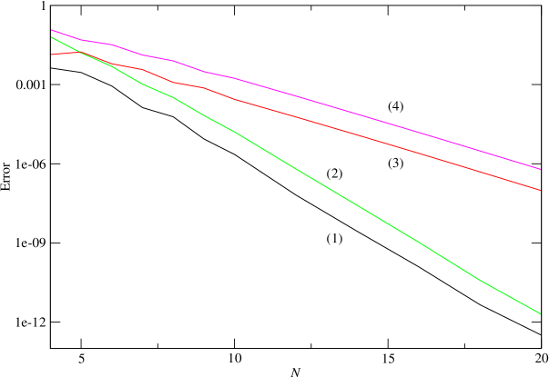
Figure 2: Results of numerical experiments for different DG implementations. Shown is the error as a function of resolution $N$ for integrating the scalar wave equation as described in the text. The numerical annotations on each line correspond to cases (1) – (4) in the text.

We find that for the analytic map used here, the results when the metric identities are satisfied are indistinguishable on the plot from the results with the analytic Jacobian. Accordingly, experiments (5) and (6) are not shown in the figure. For the analytic map, it appears that the grid distortion is small enough that the metric identity error is less than the truncation error. We explicitly computed the discrete metric identities for these cases to verify that, although they do not vanish, their magnitude is smaller than the truncation error.

The first thing we note from Figure 2 is the expected exponential convergence of the error with resolution for all the implementations. Cases (1) and (2), which use the isoparametric map, have smaller errors for the same resolution than the corresponding cases (3) and (4) that use the analytic map. As explained in the previous paragraph, this is not because the isoparametric map satisfies the metric identities. Rather, the isoparametric map introduces less grid distortion for this example. We can quantify this very roughly by examining the magnitude of the Jacobian, which is closer to unity by about a factor of 2 for the isoparametric map than the analytic map.

The most interesting result from these experiments is that, independent of the mapping, the integrate-then-transform formulation performs somewhat better than the transform-then-integrate version. The error for a given $N$ is consistently smaller for cases (1) and (3) compared with (2) and (4). It should be noted, however, that for this simple example, the computation time is dominated by the matrix-vector multiplies in computing the derivatives. For cases (1) and (3), each derivative matrix has to operate on each component of the flux vector, whereas for cases (2) and (4) each derivative matrix operates on only a single component of the flux vector. Accordingly, the computation time is twice as long (in two dimensions) for cases (1) and (3) than for cases (2) and (4). Realistic astrophysics applications are likely to be dominated by complicated equation of state calculations or source terms, so it is not clear that this property will be important in practice. Since the transform-then-integrate algorithm is widely used, whether integrate-then-transform is better just for this setup or whether it is better in general needs to be examined in future work.

Note that for this example, integrating the scalar wave equation in non-conservative form gives identical results to the conservative form studied in the experiments. This is because for linear equations with constant coefficients the matrix $A^{a}=\partial F^{a}/\partial u$ is constant and so the two formulations are essentially identical.

We have not investigated the effect of enforcing the geometric conservation law in the case where one uses a time-dependent map. There are various strategies for doing so. These strategies, and the accuracy of the resulting algorithms, are discussed for example in Ref. [23].

9 Conclusions

We have shown that because of the underlying covariance of the equations, the DG algorithm can easily be formulated in general relativity. The formulation turns out to be very similar to that for curvilinear coordinates in flat spacetime, which leads to several insights that are applicable in that arena as well.

We find that in general there are two distinct strong formulations for conservation laws. These correspond to integrate-then-transform, Eqs. (3.17) and (3.19), and transform-then-integrate, Eq. (4.12). Both weak forms are equivalent to this second strong form for the tensor-product basis functions we use. In one spatial dimension, or for the common case of a Cartesian grid with elements simply translated in $x$, $y$, and $z$, the two strong formulations are equivalent.

Most applications in curvilinear coordinates in flat space have used the formulation (4.12). However, in the numerical experiments described in §8, the other formulation was more efficient. Whether this is true or not in general remains to be seen.

For hyperbolic equations in non-conservation form, there are also two inequivalent formulations, Eqs. (5.6) and (5.9). These formulations are important for solving Einstein’s equations, which generally are not written in conservation form.

We have given a careful discussion of how numerical fluxes should be handled. In particular, we have shown that the normal vector that the boundary flux vector is projected along does not need to be the unit normal—the normalization factor cancels out of the algorithm. We call this normal vector the “outside” normal vector. If a characteristic decomposition is used to construct the numerical flux vector, it is the unit normal that appears “inside” the flux. However, it is not necessary to explicitly normalize this vector either: Any normal vector that is used in finding the characteristic decomposition gets automatically normalized “inside” the flux.

We have shown that moving grids implemented with time-dependent mappings (ALE and dual-frame methods) are easily handled in the relativistic treatment. We give a novel derivation of the ALE method that uses general covariance to get the result in a few lines. In addition, the reason that the ALE method preserves the conservation form of the equations is explained.

We clarify several aspects of the metric identities. For example, we show that satisfying the metric identities discretely is a necessary condition for free-stream preservation only for one of the computational formulations of the DG algorithm and not the other. The numerical experiments in §8 suggest that satisfying the metric identities is not necessarily a prerequisite for accurate simulations, but likely depends on the problem.

The formulation of the DG method in this paper will allow the algorithm to be applied to general problems in computational astrophysics that involve relativistic gravity. These methods hold great promise for achieving high accuracy and efficiency on current and upcoming supercomputer hardware. It will be interesting to see how well they perform in practice.

Appendix A Gauss’s Theorem and normal vectors

The usual form of Gauss’s Theorem for an arbitrary curved (or curvilinear) metric is

$$\int_{V}\nabla_{a}F^{a}\sqrt{\gamma}\,d^{3}x=\oint_{S}F^{a}\,d^{2}\Sigma_{a}=\oint_{S}F^{a}n_{a}\,d^{2}\Sigma.$$ (A.1)

This is a physically appealing result: The left-hand side is the divergence of a flux integrated over proper volume. The right-hand side is the total flux through the surface. In this form, the result is manifestly independent of the coordinates. Let’s now spoil this elegant result.

The covariant divergence in the integrand of Eq. (A.1) can be written as

$$\nabla_{a}F^{a}=\frac{1}{\sqrt{\gamma}}\partial_{a}\left(\sqrt{\gamma}F^{a}\right).$$ (A.2)

So, letting $\sqrt{\gamma}F^{a}\to F^{a}$, an equivalent form of (A.1) is

$$\int_{V}\partial_{a}F^{a}\,d^{3}x=\oint_{S}F^{a}\frac{1}{\sqrt{\gamma}}\,d^{2}\Sigma_{a}=\oint_{S}F^{a}n_{a}\frac{1}{\sqrt{\gamma}}\,d^{2}\Sigma.$$ (A.3)

We see explicitly that Gauss’s Theorem appears to depend on the metric in several places, for example, to define the unit normal $n_{a}$ and the invariant surface element $d^{2}\Sigma$. However, it turns out that this dependence is illusory, introduced originally by Stokes who first developed the geometric form of the theorem. For our application, it is actually more convenient to revert to the primitive form of the theorem that uses only basic calculus and does not rely on the metric.

Start with one of the terms on the left-hand side of Eq. (A.3):

$$I_{3} =\int\partial_{3}F^{3}\,d^{3}x$$

$$=\int\frac{\partial F^{3}}{\partial x^{3}}\,dx^{1}\,dx^{2}\,dx^{3}$$

$$=\int F^{3}\Big{|}^{x^{3}_{+}}_{x^{3}_{-}}\,dx^{1}\,dx^{2}.$$ (A.4)

Consider first the surface $x^{3}=x^{3}_{+}$. Choose intrinsic coordinates $(a^{1},a^{2})$ to parametrize this surface, so that on the surface

$$\begin{split}x^{1}&=x^{1}(a^{1},a^{2})\\ x^{2}&=x^{2}(a^{1},a^{2}).\end{split}$$ (A.5)

Extend the coordinates $(a^{1},a^{2})$ to cover the neighborhood of the surface by introducing a third coordinate $a^{3}$ such that the boundary is a level surface $a^{3}=\text{constant}$. The contribution to the integral (A.4) is

$$I_{3+} =\int F^{3}(x^{3}_{+})\,dx^{1}\,dx^{2}$$

$$=\int F^{3}\frac{\partial(x^{1},x^{2})}{\partial(a^{1},a^{2})}\,da^{1}\,da^{2}.$$ (A.6)

An alternative form can be derived using some Jacobian gymnastics:

$$\left.\frac{\partial(x^{1},x^{2})}{\partial(a^{1},a^{2})}\right|_{a_{3}} =\frac{\partial(x^{1},x^{2},a^{3})}{\partial(a^{1},a^{2},a^{3})}$$

$$=\frac{\partial(x^{1},x^{2},a^{3})}{\partial(x^{1},x^{2},x^{3})}\frac{\partial(x^{1},x^{2},x^{3})}{\partial(a^{1},a^{2},a^{3})}$$

$$=J\left.\frac{\partial a^{3}}{\partial x^{3}}\right|_{x_{1},\,x_{2}}.$$ (A.7)

(You can also derive Eq. (A.7) by noting that $\partial a^{3}/\partial x^{3}$ is an element of the inverse of the Jacobian matrix. Eq. (A.7) says that this element is given by the cofactor of $\partial x^{3}/\partial a^{3}$ divided by the determinant of the matrix.)

Substituting Eq. (A.7) in Eq. (A.6) gives

$$I_{3+}=\int F^{3}\frac{\partial a^{3}}{\partial x^{3}}J\,da^{1}\,da^{2}.$$ (A.8)

Summing up contributions like this from each segment of the boundary surface gives the simple form of Gauss’s Theorem that is in effect being used in the main text, with the identification $J\,da^{1}\,da^{2}\to J\,dx^{\bar{1}}\,dx^{\bar{2}}=dx^{1}\,dx^{2}$.

A.1 Using a metric

The form (A.6) or (A.7) does not make use of a metric. We can start to see where the usual form of Gauss’s theorem comes from by noting that the normal to the surface $a^{3}=\text{constant}$ is proportional to $(0,0,1)$ in the $(a^{1},a^{2},a^{3})$ coordinates, and so $\partial a^{3}/\partial x^{3}$ is proportional to the component $n_{3}$ in the $(x^{1},x^{2},x^{3})$ coordinates. But to write the result in terms of a true unit normal we need to introduce a metric. To do this, note that

$$\frac{\partial(x^{1},x^{2})}{\partial(a^{1},a^{2})}\,da^{1}\,da^{2} =e_{3ab}\frac{\partial x^{a}}{\partial a^{1}}\frac{\partial x^{b}}{\partial a^{2}}\,da^{1}\,da^{2}$$

$$=\frac{1}{2}e_{3ab}\,dx^{a}\wedge dx^{b}$$

$$=\frac{1}{\sqrt{\gamma}}\frac{1}{2}\epsilon_{3ab}\,dx^{a}\wedge dx^{b}.$$ (A.9)

Here $e_{abc}$ is the completely antisymmetric permutation symbol and $\epsilon_{abc}=\sqrt{\gamma}e_{abc}$ is the permutation tensor (Levi-Civita tensor). The 1-form $dx^{a}$ is defined from the parametrization of the surface, $x^{a}=x^{a}(a^{1},a^{2})$:

$$dx^{a}=\frac{\partial x^{a}}{\partial a^{1}}da^{1}+\frac{\partial x^{a}}{\partial a^{2}}da^{2}.$$ (A.10)

Define the surface element in the usual way:

$$d^{2}\Sigma_{c}=\frac{1}{2}\epsilon_{cab}\,dx^{a}\wedge dx^{b}.$$ (A.11)

This requires only a notion of volume ($\sqrt{\gamma}$). With a full metric, however, it is equivalent to

$$d^{2}\Sigma_{c}=n_{c}d^{2}\Sigma,\qquad d^{2}\Sigma=\sqrt{{}^{(2)}\gamma}da^{1}\,da^{2}.$$ (A.12)

as we will verify below. The vector with components $n_{c}$ is the normal to the surface, here assumed to be $a^{3}=\text{constant}$, and ${}^{(2)}\gamma$ is the determinant of the 2-dimensional metric induced on the surface by $\gamma_{ij}$.

A.2 Proof that $d^{2}\Sigma_{c}=n_{c}d^{2}\Sigma$

First get an expression for the normal vector. Let $x^{\bar{a}}$ denote the coordinates $(a^{1},a^{2},a^{3})$. The unit normal to the surface $a^{3}=\text{constant}$ has components

$$n_{\bar{a}}=\frac{1}{\sqrt{\gamma^{\bar{3}\bar{3}}}}(0,0,1),$$ (A.13)

where

$$\gamma^{\bar{3}\bar{3}}=\frac{\text{cofactor}(\gamma_{\bar{3}\bar{3}})}{\det(\gamma_{\bar{i}\bar{j}})}=\frac{{}^{(2)}\gamma}{\bar{\gamma}}.$$ (A.14)

Taking determinants of both sides of the transformation rule

$$\gamma_{\bar{i}\bar{j}}=\frac{\partial x^{i}}{\partial x^{\bar{i}}}\frac{\partial x^{j}}{\partial x^{\bar{j}}}\gamma_{ij}$$ (A.15)

gives the transformation rule

$$\sqrt{\bar{\gamma}}=J\sqrt{\gamma}.$$ (A.16)

Thus Eq. (A.13) becomes

$$n_{\bar{a}}=\frac{\sqrt{\bar{\gamma}}}{\sqrt{{}^{(2)}\gamma}}(0,0,1)=J\frac{\sqrt{\gamma}}{\sqrt{{}^{(2)}\gamma}}(0,0,1),$$ (A.17)

and so

$$n_{a} =\frac{\partial x^{\bar{a}}}{\partial x^{a}}n_{\bar{a}}$$

$$=\frac{\partial a^{3}}{\partial x^{a}}J\frac{\sqrt{\gamma}}{\sqrt{{}^{(2)}\gamma}}.$$ (A.18)

Now we can verify Eq. (A.12):

$$d^{2}\Sigma =n^{c}d^{2}\Sigma_{c}$$

$$=\frac{1}{2}n^{c}\epsilon_{cab}\,dx^{a}\wedge dx^{b}$$

$$=\frac{1}{2}n^{\bar{c}}\epsilon_{\bar{c}\bar{a}\bar{b}}\,dx^{\bar{a}}\wedge dx^{\bar{b}}$$ (since the quantity is a scalar)

$$=n^{\bar{3}}\sqrt{\bar{\gamma}}\,da^{1}\,da^{2}$$

$$=\gamma^{\bar{3}\bar{3}}n_{\bar{3}}\sqrt{\bar{\gamma}}\,da^{1}\,da^{2}$$

$$=\sqrt{{}^{(2)}\gamma}\,da^{1}\,da^{2} \text{(using (\ref{eq:207}) and (\ref{eq:210}))},$$ (A.19)

which is the correct expression for the surface element.

A.3 The usual form of Gauss’s Theorem

Now return to Eq. (A.6). Equation (A.9) becomes

$$\frac{\partial(x^{1},x^{2})}{\partial(a^{1},a^{2})}\,da^{1}\,da^{2}=\frac{1}{\sqrt{\gamma}}d^{2}\Sigma_{3}=\frac{1}{\sqrt{\gamma}}n_{3}\,d^{2}\Sigma.$$ (A.20)

So Eq. (A.6) can be rewritten as

$$I_{3+}=\int F^{3}n_{3}\frac{1}{\sqrt{\gamma}}\,d^{2}\Sigma.$$ (A.21)

A similar expression holds on the lower surface $x^{3}=x^{3}_{-}$ provided we interpret the normal vector as pointing in the outward direction. This is because the outward normal has components proportional to $(0,0,-1)$, but $F^{3}(x^{3}_{-})$ appears in the integrand of (A.4) with a compensating minus sign.

Similar arguments hold for the terms $I_{1}$ and $I_{2}$ analogous to (A.4). The conclusion is that Gauss’s Theorem in the form Eq. (A.3) holds in general.

To complete the proof of Gauss’s Theorem, we would need to deal with concave surfaces (above we implicitly assumed each boundary surface was convex) and also surfaces with corners, where $x_{+}$ and $x_{-}$ can be on boundary segments parametrized by different pairs of $a^{1}$, $a^{2}$, and $a^{3}$. Both these complications can be handled by subdividing the volume into subvolumes, and the details are not important for our purposes.

Appendix B The metric identities

The metric identities (4.5) follow from properties of the Jacobian matrix itself. First, an element of the inverse Jacobian matrix $\partial x^{\bar{a}}/\partial x^{a}$ is given by the cofactor of $\partial x^{a}/\partial x^{\bar{a}}$ divided by the determinant $J$. We can recover this result using some Jacobian manipulations: If $a$, $b$, and $c$ are in cyclic order, then

$$\left.\frac{\partial x^{\bar{a}}}{\partial x^{a}}\right|_{x^{b},\,x^{c}} =\frac{\partial(x^{\bar{a}},x^{b},x^{c})}{\partial(x^{a},x^{b},x^{c})}$$

$$=\frac{\partial(x^{\bar{a}},x^{b},x^{c})}{\partial(x^{\bar{a}},x^{\bar{b}},x^{\bar{c}})}\frac{\partial(x^{\bar{a}},x^{\bar{b}},x^{\bar{c}})}{\partial(x^{a},x^{b},x^{c})}$$

$$=\frac{\partial(x^{b},x^{c})}{\partial(x^{\bar{b}},x^{\bar{c}})}\frac{1}{J}.$$ (B.1)

Equivalently,

$$J\frac{\partial x^{\bar{a}}}{\partial x^{a}}=\epsilon_{abc}\frac{\partial x^{b}}{\partial x^{\bar{b}}}\frac{\partial x^{c}}{\partial x^{\bar{c}}}.$$ (B.2)

We can rewrite this equation to build in the cyclic order requirement:

$$J\frac{\partial x^{\bar{a}}}{\partial x^{a}}=\frac{1}{2}\epsilon^{\bar{a}\bar{b}\bar{c}}\epsilon_{abc}\frac{\partial x^{b}}{\partial x^{\bar{b}}}\frac{\partial x^{c}}{\partial x^{\bar{c}}}.$$ (B.3)

The metric identity follows immediately from the expression (B.3). For when we take its divergence with $\partial_{\bar{a}}$, the second derivative terms are symmetric in $\bar{a}$ and $\bar{b}$ or $\bar{a}$ and $\bar{c}$, whereas $\epsilon^{\bar{a}\bar{b}\bar{c}}$ is antisymmetric.

Note that in the general derivation given here, the elements of the Jacobian matrix cannot be interpreted as components of basis vectors in curvilinear coordinates. This is because we are not starting from a Euclidean metric.

Appendix C An identity for GLL derivative matrices

Equation (4.17) is an identity for Gauss-Legendre-Lobatto derivative matrices that is useful in converting between the strong and weak forms of the DG equations, and is also at the root of discrete “summation by parts.” The relation is implicit in the second equation following Eq. (25) in Ref. [27]. Here we demonstrate the identity explicitly.

Consider the integral on the reference element that defines the “stiffness matrix,”

$$S_{il}=\int_{-1}^{1}\ell_{i}(x)\ell_{l}^{\prime}(x)\,dx.$$ (C.1)

Integrating by parts gives

$$S_{il} =\left.\ell_{i}(x)\ell_{l}(x)\right|^{1}_{-1}-\int_{-1}^{1}\ell_{i}^{\prime}(x)\ell_{l}(x)\,dx$$

$$=\delta_{Ni}\delta_{Nl}-\delta_{0i}\delta_{0l}-S_{li}.$$ (C.2)

To get the last line, note that for the Lobatto case, all the cardinal functions must vanish at $\pm 1$ except for $\ell_{0}$ and $\ell_{N}$. Now for $N+1$ grid points, the integrand in (C.1) is a polynomial of degree $2N+1$, and so doing the integral by Gauss-Lobatto quadrature gives the exact result:

$$S_{il} =\sum_{j}w_{j}\ell_{i}(x_{j})\ell_{l}^{\prime}(x_{j})$$

$$=\sum_{j}w_{j}\delta_{ij}D_{jl}$$

$$=w_{i}D_{il}.$$ (C.3)

Substituting (C.3) in (C.2) gives the relation 4.17).

Appendix D The geometric conservation law

The geometric conservation law is an identity for the Jacobian of a time-dependent spatial coordinate transformation like (7.2). From Eq. (7.3), the Jacobian is the determinant of the spatial Jacobian matrix:

$$J=\det\mbox{$\mathbf{J}$},\qquad\mbox{$\mathbf{J}$}=\frac{\partial x^{a}}{\partial x^{\hat{a}}}.$$ (D.1)

To derive the identity, use the formula for the derivative of a determinant,

$$\partial_{\hat{t}}J =J\operatorname{Tr}\left(\mbox{$\mathbf{J}$}^{-1}\cdot\partial_{\hat{t}}\mbox{$\mathbf{J}$}\right)$$

$$=J\left(J_{ba}^{-1}\partial_{\hat{t}}J_{ab}\right)\qquad\text{(sum on $a$ and $b$)}.$$ (D.2)

Using Eq. (7.4) and replacing the index $b$ by $\hat{a}$ gives the geometric conservation law:

$$\frac{\partial J}{\partial\hat{t}} =J\frac{\partial x^{\hat{a}}}{\partial x^{a}}\frac{\partial v_{g}^{a}}{\partial x^{\hat{a}}}$$

$$=\frac{\partial}{\partial x^{\hat{a}}}\left(J\frac{\partial x^{\hat{a}}}{\partial x^{a}}v_{g}^{a}\right)\qquad\text{(using Eq.\ \ref{eq:504})}$$

$$=\frac{\partial}{\partial x^{\hat{a}}}\left(Jv_{g}^{\hat{a}}\right).$$ (D.3)

References

References

- [1] S. E. Field, J. S. Hesthaven, S. R. Lau, Discontinuous Galerkin method for computing gravitational waveforms from extreme mass ratio binaries, Class. Quantum Grav. 26 (2009) 165010.
- [2] G. Zumbusch, Finite element, discontinuous Galerkin, and finite difference evolution schemes in spacetime, Class.Quantum Grav. 26 (2009) 175011.
- [3] S. E. Field, J. S. Hesthaven, S. R. Lau, A. H. Mroue, Discontinuous Galerkin method for the spherically reduced Baumgarte-Shapiro-Shibata-Nakamura system with second-order operators, Phys. Rev. D 82 (2010) 104051.
- [4] D. Radice, L. Rezzolla, Discontinuous Galerkin methods for general-relativistic hydrodynamics: Formulation and application to spherically symmetric spacetimes, Phys. Rev. D 84 (2011) 024010.
- [5] J. D. Brown, P. Diener, S. E. Field, J. S. Hesthaven, F. Herrmann, A. H. Mroué, O. Sarbach, E. Schnetter, M. Tiglio, M. Wagman, Numerical simulations with a first-order BSSN formulation of Einstein’s field equations, Phys. Rev. D 85 (2012) 084004.
- [6] P. Mocz, M. Vogelsberger, D. Sijacki, R. Pakmor, L. Hernquist, A discontinuous Galerkin method for solving the fluid and magnetohydrodynamic equations in astrophysical simulations, Mon. Not. Roy. Astr. Soc. 437 (2014) 397–414.
- [7] O. Zanotti, M. Dumbser, A. Hidalgo, D. Balsara, An ADER-WENO finite volume AMR code for astrophysics, in: N. V. Pogorelov, E. Audit, G. P. Zank (Eds.), 8th International Conference of Numerical Modeling of Space Plasma Flows (ASTRONUM 2013), Vol. 488 of Astronomical Society of the Pacific Conference Series, 2014, pp. 285–290.
- [8] E. Endeve, C. D. Hauck, Y. Xing, A. Mezzacappa, Bound-preserving discontinuous Galerkin methods for conservative phase space advection in curvilinear coordinates, J. Comput. Phys. 287 (2015) 151–183.
- [9] O. Zanotti, F. Fambri, M. Dumbser, Solving the relativistic magnetohydrodynamics equations with ADER discontinuous Galerkin methods, a posteriori subcell limiting and adaptive mesh refinementarXiv:1504.07458.
- [10] K. Schaal, A. Bauer, P. Chandrashekar, R. Pakmor, C. Klingenberg, V. Springel, Astrophysical hydrodynamics with a high-order discontinuous Galerkin scheme and adaptive mesh refinementarXiv:1506.06140.
- [11] M. A. Scheel, H. P. Pfeiffer, L. Lindblom, L. E. Kidder, O. Rinne, S. A. Teukolsky, Solving Einstein’s equations with dual coordinate frames, Phys. Rev. D 74 (2006) 104006.
- [12] T. W. Baumgarte, S. L. Shapiro, Numerical relativity: Solving Einstein’s equations on the computer, Cambridge University Press, Cambridge, UK, 2010.
- [13] L. Rezzolla, O. Zanotti, Relativistic hydrodynamics, Oxford University Press, Oxford, UK, 2013.
- [14] A. P. Lightman, W. H. Press, R. H. Price, S. A. Teukolsky, Problem book in relativity and gravitation, Princeton University Press, Princeton, NJ, 1975, available online at http://www.nr.com.
- [15] D. A. Kopriva, G. Gassner, On the quadrature and weak form choices in collocation type Discontinuous Galerkin spectral element methods, J. Sci. Comput. 44 (2010) 136–155.
- [16] D. A. Kopriva, Implementing spectral methods for partial differential equations, Springer Science+Business Media, New York, NY, 2009.
- [17] L. Lindblom, M. A. Scheel, L. E. Kidder, R. Owen, O. Rinne, A new generalized harmonic evolution system, Class. Quantum Grav. 23 (2006) S447–S462.
- [18] M. Shibata, T. Nakamura, Evolution of three-dimensional gravitational waves: Harmonic slicing case, Phys. Rev. D 52 (1995) 5428–5444.
- [19] T. W. Baumgarte, S. L. Shapiro, Numerical integration of Einstein’s field equations, Phys. Rev. D 59 (1999) 024007.
- [20] J. Donea, A. Huerta, J.-P. Ponthot, A. Rodríguez-Ferran, Arbitrary Lagrangian-Eulerian Methods, in: E. Stein, R. de Borst, T. J. R. Hughes (Eds.), Encyclopedia of Computational Mechanics, Vol. 1, John Wiley & Sons, New York, 2004, Ch. 14.
- [21] A. H. Mroué, M. A. Scheel, B. Szilágyi, H. P. Pfeiffer, M. Boyle, D. A. Hemberger, L. E. Kidder, G. Lovelace, S. Ossokine, N. W. Taylor, A. Zenginoğlu, L. T. Buchman, T. Chu, E. Foley, M. Giesler, R. Owen, S. A. Teukolsky, Catalog of 174 binary black hole simulations for gravitational wave astronomy, Phys. Rev. Lett. 111 (2013) 241104.
- [22] J. F. Thompson, Z. U. A. Warsi, C. W. Mastin, Numerical grid generation: Foundations and applications, North-Holland, New York, 1985, available online at http://www.erc.msstate.edu/publications/gridbook.
- [23] C. A. A. Minoli, D. A. Kopriva, Discontinuous Galerkin spectral element approximations on moving meshes, J. Comput. Phys. 230 (2011) 1876–1902.
- [24] W. H. Press, S. A. Teukolsky, W. T. Vetterling, B. P. Flannery, Numerical recipes: The art of scientific computing, 3rd Edition, Cambridge University Press, Cambridge, UK, 2007.
- [25] D. A. Kopriva, Metric identities and the Discontinuous Galerkin spectral element method on curvilinear meshes, J. Sci. Comput. 26 (2006) 301–327.
- [26] J. H. Williamson, Low-storage Runge-Kutta schemes, J. Comput. Phys. 35 (1980) 48–56.
- [27] M. H. Carpenter, D. Gottlieb, Spectral methods on arbitrary grids, J. Comput. Phys. 129 (1996) 74–86.