Powerful, Rotating Disk Winds from Stellar-mass Black Holes

Abstract

We present an analysis of ionized X-ray disk winds observed in the Fe K band of four stellar-mass black holes observed with Chandra, including 4U 1630$-$47, GRO J1655$-$40, H 1743$-$322, and GRS 1915$+$105. High-resolution photoionization grids were generated in order to model the data. Third-order gratings spectra were used to resolve complex absorption profiles into atomic effects and multiple velocity components. The Fe XXV line is found to be shaped by contributions from the intercombination line (in absorption), and the Fe XXVI line is detected as a spin-orbit doublet. The data require 2–3 absorption zones, depending on the source. The fastest components have velocities approaching or exceeding $0.01c$, increasing mass outflow rates and wind kinetic power by orders of magnitude over prior single-zone models. The first-order spectra require re-emission from the wind, broadened by a degree that is loosely consistent with Keplerian orbital velocities at the photoionization radius. This suggests that disk winds are rotating with the orbital velocity of the underlying disk, and provides a new means of estimating launching radii – crucial to understanding wind driving mechanisms. Some aspects of the wind velocities and radii correspond well to the broad-line region (BLR) in active galactic nuclei, suggesting a physical connection. We discuss these results in terms of prevalent models for disk wind production and disk accretion itself, and implications for massive black holes in active galactic nuclei.

1. Introduction

X-ray disk winds from low-mass X-ray binaries (LMXBs) are revealing new facets of compact object accretion. For instance, winds carry away a significant fraction of the mass that is accreted onto the compact object. Estimates range from a few percent of the mass accretion rate in the the inner disk, to several times the inflow rate (see, e.g., King et al. 2013). This means that mass transfer even in LMXBs may be highly non-conservative in the very phase when the mass transfer rate is expected to be highest. This impacts binary evolution models, and numerous specific predictions, including e.g. the spin evolution of compact objects in LMXBs (for a review of spins, see Miller & Miller 2014; for a review of black hole X-ray binaries, see Remillard & McClintock 2006; also see Fragos & McClintock 2015).

Winds in stellar-mass black holes, in particular, may provide insights into X-ray ”warm absorbers” and faster outflows from Seyfert-1 active galactic nuclei (AGN) and quasars. Instrumental sensitivity curves and intrinsic spectral shapes make the study of low-ionization gas in warm absorbers relatively easy. This readily-detected gas could arise via irradiation of the ”torus” (e.g. Kriss et al. 1996; also see Lee et al. 2001); it may not directly probe the physics of the inner accretion disk. However, highly ionized components with potentially different origins have emerged in deep exposures. The Chandra/HETG spectrum of MCG-6-30-15, for instance, contains strong Fe XXV and Fe XXVI (He-like and H-like) absorption lines. They are blue-shifted by $v=2000$  km/s, require a column of $N_{\rm H}\simeq 3\times 10^{23}~{}{\rm cm}^{2}$, and imply a kinetic power that is about 10% of the radiative luminosity (Young et al. 2005). The inferred launching radius is $10^{3-4}~{}{\rm GM/c}^{2}$, putting this component within or interior to the broad (emission) line region (BLR). These wind properties are remarkably similar to those measured in, e.g., GRO J1655$-$40 (Miller et al. 2006, 2008; Kallman et al. 2009; Neilsen & Homan 2012). Connections like this may underlie emerging relationships between the kinetic power of winds and accretion power, that span the black hole mass scale (King et al. 2013).

Most importantly, perhaps, disk winds may reveal the fundamental physics of disk accretion, making contact with simulations in a way that continuum emission from the disk cannot. Studies have shown that disk winds and jets in X-ray binaries are anti-correlated (Miller et al. 2006b, 2008; Neilsen & Lee 2009; King et al. 2012, Ponti et al. 2012). There is actual evidence of absence: jets are truly quenched in disk–dominated soft states (Russell et al. 2010), and winds are not absent owing only to ionization effects (Miller et al. 2012). Viable explanations for this dichotomy include changes in the inner accretion disk (perhaps related to the onset of an advection-dominated accretion flow), and/or changes in dominant magnetic field component above the disk (e.g. poloidal or toroidal). More directly, some winds may be powered by magnetic forces, which points to the underlying role of magnetic fields in mediating mass and angular momentum transfer within the disk (Miller et al. 2006a, 2008).

Constraints on wind launching radii are central to understanding how the winds are driven, and how much mass and power they carry. This requires photoionization modeling of the absorbing gas. In most cases, the gas density is not known, and radii must be deduced via $r\leq L/N\xi$ (where $L$ is the ionizing luminosity, $r$ is the launching radius, $N$ is the equivalent hydrogen column density, and $\xi$ is the ionization parameter). This assumes that $N=nr$ rather than $N=n\delta r$, and in this sense it is an upper limit. In rare cases, the gas density can be measured directly, and wind radii can be derived from $r=\sqrt{(}L/n\xi)$. In the black hole GRO J1655$-$40, the ratio of Fe XXII lines at 11.87 Å  and 11.92 Å  gives a density of $n\simeq 10^{14}~{}{\rm cm}^{-3}$. (Miller et al. 2006a, 2008). In the black hole candidate MAXI J1305$-$704, these line ratios imply a density of $n\simeq 10^{16-17}~{}{\rm cm}^{-3}$ (though that wind may not escape the system; Miller et al. 2014). It is likely reasonable to assume that other winds with numerous similarities to e.g. GRO J1655$-$40 may be equally dense, but high line-of-sight column densities have prevented the detection of Fe L-shell lines in prominent sources including 4U 1630$-$472, H 1743$-$322, and GRS 1915$+$105.

Recent studies of a large population point toward an accretion disk wind origin for the BLR in AGN (Tremaine et al. 2014). Assuming that Keplerian velocities dominate the width of these optical and UV lines, radii of $10^{3-4}~{}{\rm GM/c}^{2}$ are obtained. This range is commensurate with wind radii inferred in stellar-mass black holes, again pointing to a connection. However, disk winds in black hole X-ray binaries have not previously been detected in emission, preventing a similar dynamical constraint on the launching radius. This complicates most attempts to understand the wind driving mechanism and the total mass outflow rate, and hampers a clear association with stellar-mass disk winds and the broad line region.

The best disk wind spectra have been modeled in an approximate fashion. Some analyses have attempted a line-by-line treatment with Gaussian absorption functions (e.g. Miller et al. 2006b, Kubota et al. 2007, Neilsen & Lee 2009, Ueda et al. 2009). Other efforts have made use of single-zone absorption models generated with, e.g., XSTAR (e.g. Kallman & Bautista 2001; Kallman et al. 2009) or Cloudy (e.g. Ferland et al. 1998). While this procedure is far more physically self-consistent than line-by-line fitting, and while it has likely captured the broad characteristics of disk winds correctly, it has not yielded statistically acceptable fits. It is likely that the spectra contain additional information that has yet to be exploited. Importantly, only one prior effort has included re-emission from the wind (see Miller et al. 2014, concerning MAXI J1305$-$704), which must occur whenever there is absorption.

In this work, we re-examine the best disk wind absorption spectra from Chandra/HETG observations of stellar-mass black holes. Our analysis is restricted to the Fe K band, wherein the most highly ionized gas – likely originating closest to the black hole – is contained. If stellar-mass black hole outflows are similar to Seyfert warm absorbers, then this range also carries the bulk of the mass flux (Crenshaw & Kraemer 2012). In order to best understand the atomic and velocity structures present in the first-order HEG spectra, we also consider the third-order spectra, which deliver three times higher spectral resolution. Indeed, the third-order spectra are only a factor of a few lower in resolution than anticipated spectra from Astro-H (Takahashi et al. 2010, 2014). We employ a new version of the XSTAR photoionization package to model both first- and third-order data; its spectral resolution is 20 times higher than prior versions, and it includes updated atomic data important to the Fe K band. Last, we allow for (re-)emission from the wind, with gas parameters closely tied to corresponding absorption properties.

2. Sources and Observations

We require observations with extremely high sensitivity in the Fe K band in first-order HETG spectra; this also ensures the best possible sensitivity in third-order spectra. However, for a combination of astrophysical and pragmatic reasons, HETG observations of stellar-mass black holes with strong signatures of disk winds are relatively rare. Disk winds appear to be equatorial (Miller et al. 2006a,b; King et al. 2012; also see Ponti et al. 2012), reducing the number of sources in which these outflows can be observed. Cygnus X-1 has been observed extensively with the HETG, and it displays a complex absorption spectrum (see, e.g., Schulz et al. 2002); however, this source and other high-mass X-ray binaries are not considered as the massive companion wind contaminates any signatures of a disk wind. Cir X-1 was also omitted from consideration because its wind features (Brandt & Schulz 2000) are plausibly tied to its companion.

IGR J17091$-$3624 displayed a particularly fast and powerful disk wind (e.g. King et al. 2012), but its low flux does not permit a deeper analysis. Modest sensitivity is also a general feature of neutron star low-mass X-ray binaries; in the best cases, blue-shifted absorption is sometimes detected (e.g. Ueda et al. 2004, Miller et al. 2011), but blue-shifts are tentative in other sources and spectra (e.g. 4U 1624$-$490; see Xiang et al. 2009). The HETG spectra of MAXI J1305$-$704 contain strong wind absorption features and even re-emission at long wavelengths (Miller et al. 2014), but the observation did not deliver reliable high-resolution spectra in the Fe K region owing to a pointing offset.

The set of high-inclination black holes with very high flux levels and multiple observations of disk winds is limited to four sources: 4U 1630$-$472, GRO J1655$-$40, H 1743$-$322, and GRS 1915$+$105. Even among these, not every spectrum has excellent sensitivity. We selected the observation of each source wherein the lines were best defined (e.g. where the Fe XXV and Fe XXVI line fluxes divided by their respective errors is maximal; this is distinct from the highest column density, which would still give lines with large errors at low flux or in a short expsoure). For GRO J1655$-$40, H 1743$-$322, and GRS 1915$+$105 this was possible using published measurements (e.g. Miller et al. 2008; Miller et al. 2006b; Neilsen & Lee 2009, Ueda et al. 2009). For 4U 1630$-$472, we made simple fits to multiple spectra to determine the one with the highest sensitivity. Table 1 lists the key properties of these observations, as well as an observation of GX 339$-$4 that is examined later in this work.

Previous work on the selected spectrum of GRO J1655$-$40 already points to a degree of complexity that is not captured by single-zone photonionization models. Miller et al. (2008) report that the best single-zone model for the Fe K band in GRO J1655$-$40 – model 1C in Table 3 of that work – only achieves a relatively poor fit: $\chi^{2}/\nu=2.88$. Kallman et al. (2009) and Neilsen & Homan (2012) find evidence of multiple velocity components in the spectra of GRO J1655$-$40.

The selected spectrum of H 1743$-$322 was not modeled with a photoionzation code that has an XSPEC implementation, but Gaussian models for the lines find inconsistent blue-shifts for the Fe XXV and Fe XXVI lines ($v=320\pm 160$ and $670\pm 170$ km/s, respectively; Miller et al. 2006b). This signals that a single absorbing zone is not an adequate description of the spectrum. Indeed, within Miller et al. (2006b), it is noted that the observed Fe XXV and Fe XXVI lines cannot arise in exactly the same gas. A combination of zones with different ionizations and velocities can certainly create this disparity, however.

The shifts measured via single Gaussian models for the Fe XXV and Fe XXVI lines in the selected observation of GRS 1915$+$105 are also inconsistent (see Ueda et al. 2009). The Fe XXV line shows a red-shift, possibly indicating a contribution from the intercombination line. In contrast, the Fe XXVI line shows a blue-shift. This also signals a need for multiple velocity components.

At the time of writing, the selected spectrum of 4U 1630$-$472 has not been described in detail using a photoionization code like XSTAR or Cloudy. However, it is included in a study that finds no evidence of jet-based emission lines in this source (Neilsen et al. 2014; also see Diaz-Trigo et al. 2013).

3. Data Reduction

All Chandra-specific data reduction and processing tasks were performed using CIAO version 4.6, and corresponding calibration files. Since the HEG has more collecting area than the MEG in the Fe K band, we have only made use of HEG spectra in this work. The Chandra “tgcat” facility (tgcat.mit.edu) provides calibrated first-order spectra and associated response files for gratings observations. We therefore downloaded first-order HEG spectra and their corresponding response files through “tgcat”.

At the time of writing, complete higher-order data are not provided through the “tgcat” facility, so full obserations were obtained from the Chandra archive. Calibrated spectral files are provided through the archive, but response files must be generated by the user. Response files for the third-order redistribution matrix files were generated using the tool “mkgrmf”, and these files were then used to help construct ancillary response files using “fullgarf”.

In order to achieve the best possible sensitivity, the CIAO tool “add_grating_orders” was used to combine opposing grating orders into a single spectrum. That is, the HEG$+$1 and HEG$-$1 spectra were combined into a single first-order spectrum, and the HEG$+$3 and HEG$-$3 spectra were combined into a single spectrum. The “add_grating_orders” tool also adds the ancillary response files to create a combined response files. The gratings redistribution matrix files are effectively the same for opposing orders.

We have relied on the HEG third-order data, as it provides the highest possible spectral resolution. However, it is worth noting that the HEG second-order provides spectral resolution that is twice as high as that available in first-order spectra. Depending on the sensitivity of the data, that resolution is only on the edge of being able to separate the components of the Fe XXVI $Ly-a$ line, for instance. Future work on these and other sources can make use of the HEG second-order spectra. In contrast, the MEG second-order spectra are suppressed in the HETG, in order to facilitate order sorting.

All of the observations considered in this work were obtained by running the ACIS-S array in “continuous clocking” mode, in order to prevent photon pile-up. In this mode, imaging information along the narrow axis of the array is sacrificed in order to reduce the frame time from 3.2 s to just 2.85 ms. Since the ACIS chips are medium-resolution spectrometers, accurate order sorting can still be achieved despite the loss of imaging information. The zeroth order image lands on the S3 chip, and a sufficiently high incident flux would cause frames from this chip to drop from the telemetry stream. In each of the observations, then, a “gray” filter was applied around the zeroth order position, so that only one in 10 or one in 20 incident zeroth order photons is recorded. This enables tracking of the aimpoint and the construction of the wavelength grid in the dispersed spectra, while preventing frame loss.

This mode is capable of handling incredibly bright sources without suffering photon pile-up. If imaging information could be preserved, source and background regions could be optimized to reduce background; however, background is negligble for compared to the source flux in these observations. Aspects of this observational mode are also described in detail in Miller et al. (2006b).

4. Analysis and Results

4.1. Spectral Fitting Procedure

All spectral fits were made using XSPEC version 12.8.1g (Arnaud et al. 1996). Fits to the Chandra/HETG data were made using the Churazov weighting scheme (Churazov et al. 1996). This procedure weights channels by averaging the counts in surrounding channels. Spectral regions with small errors are therefore weighted more strongly than regions with large errors. Minimization of the $\chi^{2}$ fitting statistic then depends more strongly upon well-defined lines than on relatively noisy parts of the spectrum. The default weighting scheme was used in fits made to RXTE/PCA spectra later in this work.

For dispersive spectrometers, it is natural to work in terms of wavelength – every bin has the same size, in units of wavelength. However, the future of X-ray spectroscopic instrumentation, particularly in the Fe K band, is the microcalorimeter. The natural unit for a calorimeter is energy, since every bin has the same size in units of energy. This analysis is intended to give the very best view of accreting black holes as the field heads into the era of calorimeters with Astro-H and Athena, so we have chosen to present our analysis and results in energy units. The data were analyzed in their native bins and the results do not depend on whether energy or wavelength units are adopted.

All fits to the first-order spectra of 4U 1630$-$472, GRO J16554$-$40, H 1743$-$322, and GRS 1915$+$105 were made over the 5–10 keV range. Fits to the third-order spectra of these black holes were made over the 5–8 keV band, owing to a lack of signal and instrumental residuals above 8 keV. Where other sources and instrumental spectra are considered, the fitting band is noted explicitly in the text.

4.2. Initial Fits

To give a view of potential structure and complexity in the Fe K band, we fit each of the first-order spectra in the 5–10 keV band with a phenomenological disk black body (“diskbb”; Mitsuda et al. 1984) plus power-law model, modified by Galactic absorption fixed at standard values. This was accomplished using the “tbabs” model with appropriate cross sections and abundances (Wilms, Allen, McCray 2000). The power-law index was fixed to previously published values in each case, where simultaneous RXTE observations had been made (GRO J1655$-$40: $\Gamma=3.5$, Miller et al. 2008; GRS 1915$+$105: $\Gamma=3.0$, Ueda et al. 2009; H 1743$-$322: $\Gamma=2.4$, Miller et al. 2006b).

Figure 1 shows the data/model ratios obtained when the first-order spectra are fit with these fiducial continua. Blue-shifted Fe XXV and Fe XXVI absorption lines are the hallmarks of accretion disk winds in stellar-mass black holes, and they dominate the ratios. However, on this relatively narrow wavelength range, at least some of the lines are not simple. The Fe XXV line in the spectrum of H 1743$-$322 appears to be asymmetric, and the Fe XXVI line may show an extended blue wing. In 4U 1630$-$472, the Fe XXV line shows some evidence of complexity, and the Fe XXVI line again shows some possible structure. The Fe XXV absorption in the spectral ratio from GRS 1915$+$105 shows very clear structure, and the Fe XXVI line again shows extension to high energy. The ratio from GRO J1655$-$40 may show the most absorption structure, with different lines or velocity components potentially contributing to both Fe XXV and Fe XXVI lines.

Beyond structure in the Fe XXV and Fe XXVI absorption lines, this quick comparison of first-order spectra reveals the possibility of emission lines. It was previously noted that the absence of strong, narrow emission lines indicates that the disk winds in these high inclination sources must be equatorial: if the gas were distributed in a more spherical manner, gas above the line of sight would contribute prominent emission (Miller et al. 2006a,b). However, for any plausible geometry, some re-emission from gas outside of our line of sight should be detected. Close scrutiny of this narrow window around the Fe K region may indicate such emission, with a structure that may be broadly consistent between the source spectra. The putative emission is most prominent to the red of the strong absorption lines; the ratios are flatter above 7 keV. The structure is at least qualitatively consistent, then, with the P-Cygni profiles expected from an accretion disk wind (e.g. Dorodnitsyn & Kallman 2009, Dorodnitsyn 2010, Puebla et al. 2011).

Figure 2 shows the data/model ratios obtained from the third-order spectra of 4U 1630$-$472, H 1743$-$322, GRO J1655$-$40, and GRS 1915$+$105. The spectra were fit with the same fiducial continuum models used to characterize their corresponding first-order spectra. Particularly in GRS 1915$+$105 and GRO J1655$-$40, it is apparant that the Fe XXV line structure is indeed the result of multiple distinct lines that are blurred together at first-order resolution. This is less distinct in 4U 1630$-$472, and unclear – if present at all – in the third-order spectrum of H 1743$-$322.

Though often treated as a single line even at first-order HEG resolution, the Fe XXVI line is actually a doublet owing to spin-orbit coupling. The expected separation of the two lines is about $0.02~{}keV$ (6.952 keV and 6.973 keV, in a roughly 1:2 ratio of oscillator strengths; see Verner, Verner, & Ferland 1996). This splitting is revealed for the first time in GRO J1655$-$40. Indeed, one line pair is evident just below 7 keV, and a second just above 7.0 keV, signaling an absorption zone with an blue shift in excess of 0.01$c$. The ratio of the line fluxes is inconsistent with 1:2; this likely owes to saturation.

To quickly assess the significance of the lines in the putative doublets in GRO J1655$-$40, we added Gaussian lines to the continuum model. A velocity width of 300 ${\rm km}~{}{\rm s}^{-1}$ was assumed as per Miller et al. (2008). Dividing the Gaussian line flux by its error gives one measure of line significance. In the lower-velocity pair, the lines are each significant at the $5\sigma$ level; in the higher-velocity pair, the lines are each significant at the 3$\sigma$ level. The spectra of 4U 1630$-$472 and H 1743$-$322 show weaker evidence of having resolved the Fe XXVI doublet. The splitting is not evident in GRS 1915$+$105, but asymmetry is evident, again signaling multiple outflow components at the highest possible resolution.

Figure 3 shows the first-order ratio spectra, plotted on top of the higher-resolution third-order spectra. The asymmetries and complexities of the first-order line profiles generally correspond to individual lines in the third-order spectra. In short, the third-order spectra contain a measure of precise information that can be utilized to better understand the disk wind in these black holes.

In view of these results, we proceeded to: (1) model the third-order spectra in detail to obtain additional constraints on gas properties and velocities, and (2) combine third-order information and corresponding emission components to model the sensitive first-order spectra. Both steps necessitated the development and application of new photoionization models and fitting procedures, as described below.

4.3. Photoionization grids and model implementation

A sensible physical description of these spectra requires photoionization modeling. We generated large grids of synthetic spectra using an update to a recent public version of the XSTAR package (version 2.2.1bn19; e.g. Bautista & Kallman 2001, Kallman et al. 2009). In order to take advantage of the third-order HEG spectra, and in order to make optimal use of first-order spectra, two specific improvements were made:

$\bullet$ Prior versions of XSTAR only allowed for 10,000 spectral bins; however, this is insufficient for comparison to third-order HETG spectra. For instance, this resolution blends the Fe XXVI doublet into a single feature. The synthetic spectra in our grids were all generated using 200,000 spectral bins. This reveals all of the lines in full detail and is suited to the resolution of the third-order spectra.

$\bullet$ Improved atomic data for He-like Fe XXV intercombination lines was included. Prior versions of XSTAR under-estimated the strength of this feature, driving fits toward false velocity shifts and ionization parameters in order to model the Fe XXV intercomination line in terms of Fe XXIV absorption. Fits with the updated version of XSTAR used in this work correctly account for the intercombination line in the Fe XXV complex, and deliver more accurate gas parameters. Line wavelengths and oscillator strengths for the fine struture components of the He-like and H-like ions in the updated version of XSTAR were taken from the NIST database (physics.nist.gov/PhysRefData/ASD/lines_form.html). Only the updates to the intercombination line data are important for our analysis.

Table 2 lists the critical input parameters used to generate XSTAR grids using the “xstar2xspec” functionality. The XSPEC fitting package recognizes the grids as models and can interpolate between grid points to find the gas parameters that best correspond to the observed spectra. For each source, the grids spanned a range of $3\leq{\rm log}(\xi)\leq 6$ and $21\leq{\rm log(N)}\leq 23.8$. All grids were generated assuming a gas density of $n=10^{14}~{}{\rm g}~{}{\rm cm}^{-3}$, drawing upon the cases where the density has been measured directly. Whenever possible, parameter values – especially disk temperature and source luminosity – were taken from values in the literature. Solar abundances were used for all sources apart from GRS 1915$+$105, wherein an enhanced iron abundance has sometimes been reported (e.g. Lee et al. 2002; XSTAR takes abundances from Grevesse, Noels, & Sauval 1996). A covering fraction of $\Omega/4\pi=0.2$ was used for GRO J1655$-$40 based on prior work (Miller et al. 2008); a value of 0.5 was used for the other sources, consistent with King et al. (2013).

Though the observed spectra are best characterized by a combination of disk blackbody plus power-law models, the XSTAR grids were generated using only a simple blackbody function with an equivalent temperature. This is a simplification that introduces a degree of error and inconsistency. Model 1c in Table 3 of Miller et al. (2008) provides the most useful point of comparison, for evaluating the degree to which measurements are skewed by ignoring the power-law component. The prior work uses a lower-resolution photoionization grid, containing older atomic data. However, comparing values of column density, ionization, velocity, mass outflow rate, and kinetic power derived Miller et al. (2008) to those found in the simplest fits later in this work, the maximal systematic error induced by ignoring a power-law component may be a factor of $\simeq$2 in column density and ionization, but only 50% in radius, mass outflow rate, and kinetic power, since differing values partly compensate for each other. The true level of systematic error is likely lower, since numerous factors changed between the 2008 analysis and this paper, and some of those must also contribute to the differences.

The “xstar2xspec” script produces three distinct files for potential inclusion in XSPEC modeling: a multiplicative table model (“xout_mtable.fits”) that imprints absorption onto a continuum, an emission model that is the line spectrum emitted in all directions as a result of the initial absorption (“xout_ain.fits”), and an emission component that represents the emission lines transmitted into the pencil beam through which the absorption is seen (“xout_aout.fits”). The last component is expected to be negligible, and was not included in our models.

It may be possible to construct geometries and viewing angles that would cause the observed re-emission from an absorbing wind to sample a different set of gas properties than probed by the bulk of the absorption. However, assuming that the properties of the emitting gas are the same as the absorbing gas permits a degree of simplicity. Thus, in all spectral fits presented in this work, the equivalent neutral hydrogen column density of the gas ($N_{\rm H}$) and the ionization parameter ($\xi$) were linked, creating distinct zones with characteristic gas properties for both the absorbing and emitting gas.

The emission component carries a flux normalization parameter: ${\rm K}=f{\rm L}_{tot,38}/d_{kpc}^{2}$, where $f=\Omega/4\pi$ is the covering fraction, ${\rm L}_{tot,38}$ is the total luminosity of the source in units of $10^{38}~{}{\rm erg}~{}{\rm s}^{-1}$, and $d_{kpc}$ is the distance in units of kpc. A value of unity would indicate that each parameter has been estimated with excellent accuracy, but modest fractional errors in one or more parameters are likely, and can lead to large deviations from unity. In particular, distances within the Milky Way are often particularly uncertain, and luminosity estimates can vary depending on the spectral model assumed and the energy band over which the flux is measured. In our fits, then, the value of each emission component was loosely bounded: $0.1\leq{\rm K}\leq 10$. This range acknowledges plausible uncertainties while demanding a minimum contribution from the emission component.

Basic assumptions about the gas geometry further informed the manner in which the spectral models were constructed. The absorption lines are clearly blue-shifted; else they could not be described as disk winds. The photoionized absorption components were therefore bounded from below to have either zero velocity shift, or a blue shift. The photoionized emission lines are likely come from the full cylinder in which the disk wind arises; in this case, velocities should cancel and the emission should have zero net velocity shift (but a significant velocity width). If the far side of the cylinder (with respect to the central engine) contributes preferentially for any reason, the emission would have a net red-shift. Figures 1 and 3 suggest that any emission is strongest to the red of the (blue-shifted) absorption components. Based on these expectations, we bounded the emission components to have a red-shift between zero and the absolute value of the observed blue-shift in the same component (e.g. $v_{emis.}\leq-1.0\times v_{abs.}$). Note that when these conditions were relaxed, emission components were not found to be blue-shifted, and absorption components were not found to be red-shifted. Rather, this step merely permitted a degree of simplicity in constructing models.

A particular detail of the photoionization model implementation had to be determined via numerous fitting experiments. A priori, it is not clear if the photoionized emission spectrum from points around the wind cylinder might also be affected by local or ambient wind absorption. Numerous trials revealed that vastly improved fits are obtained when the emission spectrum is not obscured.

Last, we allowed for a narrow Gaussian emission line at 6.4 keV, consistent with emission from neutral or nearly-neutral Fe, to describe any remaining illumination of distant or ambient cold gas. Reflection from the outer disk, for instance, might be one means by which such a feature could be generated. It is unlikely that any such emission would be closely tied to the wind, and including this Gaussian allows the XSTAR models to fit ionized wind features, as intended.

For a single zone, then, the full continuum plus photoionization model was implemented into XSPEC in the following manner:

$tbabs\times((abs\times(gauss+diskbb+powerlaw)+emis)$.

Models for the spectra requiring 2–3 zones are implemented as follows:

$tbabs\times((abs_{1}\times abs_{2}\times(gauss+diskbb+powerlaw)+emis_{1}+emis_{2})$.

Further fits explored potential broadening of the photoionized emission components, using smoothing functions to model velocity broadening of the line spectrum. Simple Gaussian broadening was explored using the “gsmooth” model, bounding the maximum smoothing to 0.2 keV (at 6 keV) with an index of $\alpha=0$ (smoothing is not a function of energy):

$tbabs\times((abs\times(gauss+diskbb+powerlaw)+gsmooth\times emis)$.

Broadening with a line function that includes Doppler shifts and illumination effects was implemented using the “rdblur” function, which is a convolution model based on the “diskline” function (Fabian et al. 1989). This function is not technically appropriate for spinning black holes. However, Schwarzschild and Kerr metrics are very similar far from the black hole, and this analytic blurring model has the advantge of easily extending to large radii. An outer radius of $10^{5}~{}r_{g}$ was fixed in all cases. An emissivity index of $q=-3$ was used ($J\propto r^{q}$ in “rdblur”), appropriate for large distances from a corona (see, e.g., Wilkins & Fabian 2012). The inclination parameter within “rdblur” was constrained based on limits derived for the inner disk, in order to allow for a flared wind geometry. The final model was implemented exactly as per “gsmooth”:

$tbabs\times((abs\times(gauss+diskbb+powerlaw)+rdblur\times emis)$.

4.4. Fits to the third-order spectra

Figures 4–7 show fits to the third-order spectra of GRO J1655$-$40, GRS 1915$+$105, 4U 1630$-$472, and H 1743$-$322, approximately ordered from most complex to least complex. Each spectrum is shown with the best-fit model given in Tables 3–7 (models 1655-3a, 1915-3a, 1630-3a, 1743-3a). The spectra were “unfolded” in a manner that removes the instrumental effective area curve, without falsely imprinting the model upon the data (e.g. the XSPEC command “setplot area” was used, rather than plotting an unfolded spectrum, which serves to multiply by the ratio residuals). In this representation, it is especially clear that the Fe XXV and Fe XXVI lines contain appreciable substructure, hinted at in the first-order spectra.

Table 3–7 give the continuum and photoionization component parameters for the fits made to each source, guided by the constraints detailed above. Errors (1$\sigma$ confidence levels) are given for the best-fit model in each table. Error assessment was extremely time intensive, so errors are not given for inferior models. However, the $\chi^{2}$ fit statisic is quoted for every model, so that the improvements obtained from adding components or complexity can be assessed.

GRO J1655$-$40 can be taken as an example (see Figure 4 and Table 3). Model 1655-3a achieves the best overall $\chi^{2}$ value ($\chi^{2}/\nu=1135/1098=1.033$); it includes 3 photoionization components, all blurred by Gaussian functions. Model 1655-3b details the effect of removing one photoionization component (one paired absorption/emission zone), and fitting again. The fit is clearly only marginally worse without a third photoionization component. Similarly, model 1655-3c removed the blurring functions that acted upon the photoionized emission, and again only a marginally worse fit is achieved. From this, we can gather that only two components are strongly required in the third-order spectrum of GRO J1655$-$40, and that blurring is also not a strong requirement at this sensitivity. However, model 1655-3d removes another paired absorption/emission zone, and the fit is significantly worse ($\chi^{2}/\nu=1172/1109=1.058$). Comparing 1655-3d to all of the others, it is clear that the second zone latches onto a highly ionized, high-velocity component, with $v/c=-0.0118(5)$. In Figure 4, the Fe XXVI doublet is evident at lower velocity, closer to its rest-frame energy; above 7.0 keV, another doublet split by  20 eV is evident, and this is the second, higher-velocity component found by the fit.

Models for the third-order spectrum of GRS 1915$+$105 achieve qualitatively similar results (see Figure 5 and Table 4). The overall best-fit model includes three photoionization zones, each blurred with a Gaussian function; however, the improvement over a model including only two zones and no blurring is only marginal at this sensitivity. At least as measured in the third-order spectrum of GRS 1915$+$105, the disk wind is considerably slower than that launched in GRO J1655$-$40.

The sensitivity in the third-order spectra of 4U 1630$-$472 (see Figure 6 and Table 5) and H 1743$-$322 (see Figure 7 and Table 6) is lower than that achieved in GRO J1655$-$40 and GRS 1915$+$105. In the case of 4U 1630$-$742, two photoionization zones are only modestly preferred over a single zone. Two zones do not provide a significant improvement over a single zone in fits to H 1743$-$322, though this is the least sensitive spectrum in our sample.

For both GRO J1655$-$40 and GRS 1915$+$105, it is particularly important to note the success of the improved, high-resolution XSTAR grids. In both cases, the Fe XXV intercombination and resonance lines are correctly modeled in absorption (see Figures 4 and 5). In GRO J1655$-$40 in particular, the model correctly reproduces the 20 eV spin-orbit splitting of the Fe XXVI line. Similar structure is likely present in the spectrum of GRS 1915$+$105 as well, as the Fe XXVI line is asymmetric, but the splitting is likely partly obscured by velocity components that overlap. Evidence of complex atomic structure in the third-order spectra of 4U 1630$-$472 and H 1743$-$322 (see Figures 6 and 7) is less clear than in GRO J1655$-$40 and GRS 1915$+$105, but hints of the Fe XXV intercombination line in absorption line are evident in 4U 1630$-$472, and structure may be evident in the Fe XXVI lines of both sources.

It must be noted that the ratio of Fe XXV intercombination and resonance lines shows evidence of saturation, consistent with the gas properties that emerge from the fits (see below). For weak lines, the intercombination line is only about 10% as strong as the resonance line, based on a ratio of their oscillator strengths. The fact that the intercombination line appears to be a few times stronger than this expectation is simply the result of saturated line absorption, providing a valuable constraint on the Fe XXV column density.

In summary, the third-order spectra have limited sensitivity; however, they have verified the need for improved atomic data and higher resolution grids. The spectra establish a statistical basis for multiple absorption zones (or, velocity components) even at the highest possible spectral resolution. There are even weak hints of photoionized emission that might be broadened. These are the general lessons that we carry forward in subsequent modeling of the more sensitive first-order spectra (see below). In the case of GRO J1655$-$40, the third-order spectrum makes the presence of a highly ionized, high-velocity zone clear; this component explains curvature on the blue side of the first-order Fe XXVI line profile (see Figures 1–3), so we carry forward the velocity measured from the third-order absorption spectrum in subsequent fits to the first-order spectrum.

4.5. Fits to the first-order spectra

New fits to the first-order spectra of GRO J1655$-$40, GRS 1915$+$105, 4U 1630$-$472, and H 1743$-$322 are detailed in Tables 7–10, and the best-fit model for each spectrum is shown in Figures 8–12. The best-fit model for each source is listed first in these tables, with the suffix “-1a”. Models listed below the best-fit case explore the effects of removing different model components in order to demonstrate the statistical requirement for different levels of complexity. Here again, full errors are given for every component of the best-fit model for each first-order spectrum, but errors were not calculated for inferior models (though the resultant fit statistic is given).

Figures 8 and 9 may be compared directly in order to appreciate the improvement achieved by allowing for multiple velocity components and corresponding photoionized emission. Figure 8 shows the first-order spectrum of GRO J1655$-$40, fit with the best-fit model published in Miller et al. (2008). That model includes only one absorption zone, and no photoionized emission. Although it captures the general character of the Fe K absorption lines, the data/model ratio clearly establishes the need for a better approach. In a statistical sense, the model is also quite poor: $\chi^{2}/\nu=1555/498=3.180$ (note that the fitting band is not exactly the same as that considered in Miller et al. 2008). In strong contrast, the best-fit model from Table 7 (model 1655-1a) is shown in Figure 9; it achieves a vastly improved fit: $\chi^{2}/\nu=634/475=1.315$. The latter model is far more complex, but the statistical improvement (over $19\sigma$) is large enough to justify this complexity.

This best-fit model for the first-order of GRO J1655$-$40 requires three paired photoioinized absorption/emission zones, and blurred emission. The velocity of the most blue-shifted absorption component is fixed to $v/c=11.8\times 10^{-3}$, based on fits to the third-order spectrum. The three components follow a sequence such that column density and the absorption outflow velocity are anti-correlated. The photoionized emission components are not found to be red-shifted, consistent with expectations, but broadening of these components is strongly required (compare 1655-1a and 1655-1b; an F-test indicates the improvement is significant at more than $13\sigma$). It is notable that the two slower components require the maximum allowed broadening ($\sigma=0.2$ keV), whereas the fastest and most ionized component requires the least broadening ($\sigma=0.03\pm 0.01$ keV). Broadening is actually more important than the addition of a third photoionization zone, in a statistical sense, though the third component is nominally significant at more than the $7.6\sigma$ level of confidence (compare 1655-1a and 1655-1d).

Fits to the first-order spectrum of GRS 1915$+$105 are detailed in Table 8, and the best-fit model for the spectrum is shown in Figure 10. Similar to 1655-1a, the best fit model – 1915-1a – requires three photoionization absorption/emission pairings. None of the blue-shifted absorption components are found to flow as quickly as the fastest component in GRO J1655$-$40. Indeed, the component with the highest column density has a small outflow velocity ($v/c=0.2^{+0.1}_{-0.2}\times 10^{-3}=60_{-60}^{+30}$ km/s). The highest velocity component is also the most ionized, again similar to GRO J1655$-$40, and it is measured to have an outflow velocity of $v/c=8.0\pm 0.2\times 10^{-3}=2400\pm 600$ km/s).

In the first-order spectrum of GRS 1915$+$105, there is again evidence that the photoionized emission pairs for the stronger absorption must be broadened. Model 1915-1b removes Gaussian smoothing functions from the fit; comparing 1915-1b to 1915-1a, broadening is required at the $11.2\sigma$ level of confidence via an F-test. The requirement for three zones, rather than just two, is also strong: model 1915-1d considers only two zones, and 1915-1a is superior at more than the 5$\sigma$ level of confidence.

Fits to the first-order spectrum of 4U 1630$-$472 are detailed in Table 9, and the best-fit model (1630-1a) is shown in Figure 11. In constrast to GRO J1655$-$40 and GRS 1915$+$105, the spectrum of 4U 1630$-$472 requires only two paired photoionization absorption and emission components. However, the same general trend is recovered: the component with the highest column density has a lower blue-shift and is less highly ionized, and while the second component has a lower column density, it is more highly ionized and has a higher blue-shift. These broad similarities betwen the black hole winds may signal common properties and common launching radii and mechanisms. The slower absorption component in 4U 1630$-$472 has a velocity of $v/c=-0.9\pm 0.2\times 10^{-3}=-270\pm 60$ km/s), and the second absorption component has a velocity of $v/c=-7.0^{+3.0}_{-2.0}\times 10^{-3}=-2100^{+900}_{-600}$ km/s). The emission components paired to each of these absorption components are not required to be red-shifted.

Comparing models 1630-1a and 1630-1b, broadening of the photoionized emission components is required at the $5.7\sigma$ level of confidence, via an F-test. The requirement for photoionized emission is also lower; comparing 1630-1c with 1630-1a shows that the addition of emission components is only significant at the $3\sigma$ level of confidence. However, this likely under-predicts the actual significance of these components, as broadening may be important to evaluating the action of emission within the fit. There are different ways to evaluate the improvement achieved by considering two zones rather than just one; depending on the specific models compared, the improvement can be as low as $2\sigma$. However, based on the broad similarities in the properties of the components seen in GRO J1655$-$40, GRS 1915$+$105, and 4U 1630$-$472, it is likely that the emission components are real and stem from the same geometric considerations. Moreover, the observation of 4U 1630$-$472 did not register the same high flux level as recorded in GRO J1655$-$40 and GRS 1915$+$105; stacking observations of 4U 1630$-$472 woud likely serve to boost the significance of the emission, but lies beyond the scope of this paper.

The first-order spectrum of H 1743$-$322 is likely the simplest of those considered, likely owing only to the fact that the column density of the wind in this source is lower than in the other three. In Figure 1, the Fe XXV and XXVI lines profiles appear to be asymmetric. A superposition of Fe XXV intercombination and resonance lines from a single absorbing component would create a composite line at first-order resolution that is asymmetric in the opposite sense (stronger in a false “blue” wing). The sense of the observed asymmetry, and the explicit blue wing in the observed Fe XXVI line profile signal multiple photoionization/velcity components in the obseved disk wind.

Model 1743-1a in Table 10 includes two paired photoionization components. The fit achieved with this model is shown in Figure 12. The lower velocity absorption component is outflowing at approximately $300\pm 90$ km/s, the second component has a blue-shift of $2100^{+900}_{-600}$ km/s. The lower-velocity absorption component carries a lower column density and a lower ionization parameter than the high velocity component. The high velocity, column density, and ionization of the second component signal that it carries more mass flux, and transmits more kinetic power. The higher velocity component is not strongly required via an F-test comparing 1743-1a and 1743-1d. However, a fit to the Fe XXVI complex with two Gaussians suggests that the higher-velocity component is signficant at the $3\sigma$ level of confidence. This spectrum is consistent with broadening of the re-emission spectrum, but it is not statistically required at this low sensitivity.

4.6. Radius-focused Photoionization Modeling

Some of the (re-) emission components found in the prior fits require significant blurring, up to $\sigma\simeq 0.2$ keV. At an energy of 6.7 keV, this translates to a speed of $0.03c$, or the Keplerian orbital velocity at $r\simeq 1000~{}{\rm GM/c}^{2}$. Prior photoionization modeling of GRO J1655$-$40 found similar launching radii, and indeed similar radii are implied for several of the components reported in this work. However, it is important that all components be modeled as carefully as possible in all aspects, in order to derive the most accurate dynamical information.

At low resolution, and/or low sensitivity, Gaussian functions may be sufficient to describe the emission line profile expected at $r\simeq 1000~{}{\rm GM/c}^{2}$. However, the line profile should actually be asymmetric, primarily owing to Doppler shifts. Gravitational red-shifts may also be detectable, but this would require exquisite data. In order to better explore the ability of the data to reveal the launching radius through Doppler broadening of its re-emitted spectrum, we replaced the Gaussian functions in fits to the first-order spectra with the “rdblur” function (Fabian et al. 1989).

The “rdblur” model has important advantages over more recent models, though it has lower resolution. Models such as “kerrconv” (Brenneman & Reynolds 2006) and “relconv” (Dauser et al. 2012) only extend out to $r=400~{}{\rm GM/c}^{2}$ and $r=1000~{}{\rm GM/c}^{2}$, respectively. In contrast, “rdblur” is analytic (meaning that it runs quickly; it is based on “diskline”; Fabian et al. 1989) and can extend out to $r=10^{5}~{}{\rm GM/c}^{2}$, and beyond. The “rdblur” model assumes a Schwarzschild black hole, but differences between the Schwarzshild and Kerr metrics are negligible at the radii of interest. For simplicity, we assumed a “standard” single power-law emissivity profile of $J\propto r^{-3}$. The local gas will emit isotropically, in an $r^{-2}$ fashion. We have modeled the absorption zones assuming a constant density, which again argues for a $r^{-2}$ emissivity. In strict terms, though, the wind may have a $r^{-2}$ density profile, requiring an overall $r^{-4}$ emissivity with radius. However, much of the absorption occurs in the inner portion of a gas with a falling density profile. Overall, $r^{-3}$ is a reasonable estimate, intermediate between two reasonable possibilities. This profile is found in simulations of re-emission from a central source (Wilkins & Fabian 2012). Last, a hard lower limit of $500{\rm GM/c}^{2}$ was enforced in the fits.

The results of fits to the first-order spectra with “rdblur” replacing Gaussian blurring functions are given in Table 11. In a statistical sense, the best fits with this model are comparable to those with the Gaussian funtions (see Tables 7–10). Models with $-r1$ appended constrain the radius of all paired absorption/emission zones to be the same. These models could be considered a column density-weighted average. Models with $-r2$ appended allow each photoionized emission zone to have an independent best-fit radius. Only the spectra of GRO J1655$-$40 and GRS 1915$+$105 have the sensitivity required to make such fits. It is important to note that Table 11 only gives the $1\sigma$ errors on every fit parameter, including inner radii (in keeping with other errors in this work). The range of radii covered by $3\sigma$ confidence limits is generally a few times larger than the $1\sigma$ limits.

The radius-focused models in Table 11 are the most physical fits presented in this work. Figure 13 shows the relative importance of absorption and emission in the spectra, and evidence of disk-like P-Cygni profiles, based on the models in Table 11. In Figure 13, the photoionization components were removed from the total model for each spectrum, leaving the ratio to the direct continuum emission. The total model including photoionization components is then plotted through each ratio, to show the interplay of absorption and emission.

4.7. Launching Radii and Outflow Properties

Table 12 lists the estimated mass outflow rates and kinetic luminosities for the best models in Table 11. In all cases, the mass outflow rate was calculated via $\dot{M}_{wind}=\Omega\mu m_{p}vL/\xi$, and the kinetic power was calculated via $L_{kin}=0.5\dot{M}v^{2}$ (where $\Omega$ and $L_{rad}$ are covering fraction and radiated luminosity given in Table 2, the ionization parameter $\xi$ was measured using the XSTAR grids, $\mu$ is the mean atomic weight and $\mu=1.23$ was assumed, $m_{p}$ is the mass outflow rate, and $v$ is the measured blue-shift of each component). Eddington-scaled quantities are tabulated assuming an accretion efficiency of $\eta=0.1$ in the simple equation $L_{rad}=\eta\dot{M}c^{2}$. In all cases, a luminosity uncertainty of 50% was included to estimate outflow parameters, to account for uncertainties in source mass, distance, and continuum model.

These calculations assumed a volume filling factor of unity, and in that respect they represent a kind of upper limit. The wind may be clumpy, but there is no evidence of strong short-term variations that would suggest clumping. Indeed, the relative stability of the absorption lines in GRO J1655$-$40 has even been utilized to constrain the parameters of the binary system (Zhang et al. 2012; however, see Madej et al. 2014). Where variability has been observed in wind aborption spectra, it appears to be more closely tied to changes in the incident ionizing flux (e.g. Miller et al. 2006b) and/or changes in large-scale geometry (Ueda et al. 2009, Neilsen et al. 2012a,b), not tied to clumpiness. In contrast, the clumpiness of the companion wind in Cygnus X-1 is partly indicated by the distribution of strong X-ray flux dips with orbital phase (e.g. Wen et al. 1999).

The most ionized components in the wind do not necessarily carry the greatest mass flux, but they do account for the greatest part of the kinetic luminosity of the wind from each black hole. The mass outflow rates do not exceed the inferred mass inflow rate, but in some cases the ratio approaches $\dot{M}_{wind}/\dot{M}_{accr}\simeq 0.3$ (e.g. zone 2 for 1915-r2 in Table 12). In total, the total mass flux and kinetic power carrried by the wind from each black hole generally exceed prior estimates (e.g. King et al. 2013) by an order of magnitude, or more. This owes to the higher-velocity components detected in our modeling of the spectra, since the mass flux goes as $v$ and the kinetic power goes as $v^{2}$.

On a componenent-by-component basis, Table 12 compares the radius derived from photoionization modeling, $r_{phot}=\sqrt{(L/n\xi)}$, to the radius derived from broadening of the emission line spectrum. The radii derived from modeling the emission lines are generally slightly smaller than those derived from photoionization modeling, but the two measures generally agree to within a factor of a few. Especially in view of the numerous uncertainties and issues related to modeling the gas, this level of agreement is encouraging. It is consistent with a scenario wherein the wind retains much of the rotation of the underlying disk, meaning that broadened (re-)emission spectra can be used to estimate radii. If this is correct, then the winds are very close to the local escape speed.

This is merely an initial attempt at such modeling, and some inconsistencies remain. Factoring in errors, the most substantial discrepancy exists for “zone 1” in 1915-r2, where $r_{phot}=17,000\pm 3000{\rm GM/c}^{2}$, whereas $r_{blur}=1200^{+600}_{-200}{\rm GM/c}^{2}$. This component is among the slowest detected in our sample ($v=-0.001c$), and it also has a fairly modest ionization (log $\xi$ = $4.10\pm 0.05$). The photoionization radius of this component could be brought into closer agreement with its dynamical radius by modeling with a higher gas density.

None of the components described by Tables 11 and 12, nor indeed those detailed in Tables 3–10, can be driven through radiation pressure. The gas is simply too highly ionized for a force-multiplier effect (e.g. Proga 2003). Similarly, the optical depth to electron scattering is too low for even the components with the highest column densities to be driven in that manner. This leaves only thermal driving and magnetic forces as viable means of expelling the observed winds.

Thermal winds can be driven from the Compton radius, given by $R_{C}=(1.0\times 10^{10})\times(M_{BH}/M_{\odot})/T_{C8}$ (where $T_{C8}$ is the Compton temperature in units of $10^{8}$ K), or perhaps from $0.1~{}R_{C}$ (Begelman et al. 1983, Woods et al. 1996). Approximating the Compton temperature by the disk blackbody color temperature in Table 2, the smallest Compton radius inferred for any source is $R_{C}\simeq 4.4\times 10^{11}~{}{\rm cm}$. This corresponds to $4\times 10^{5}~{}{\rm GM/c}^{2}$ for GRO J1655$-$40, or about $3\times 10^{5}~{}{\rm GM/c}^{2}$ for the other sources. Even if a thermal wind can be driven from $0.1R_{C}$, this is still an order of magnitude larger than the radii estimated in our spectral fits. Theoretical work on thermal winds is ongoing, and recent work has found that such winds may be denser and faster than previously recognized (e.g. Higginbottom & Proga 2015), but the results of our analysis appear to confirm a role for magnetic driving.

The ratio of wind kinetic luminosity to radiated lumonsity is also given in Table 12, in units of $10^{-3}$. In this metric, the outflow from GRO J1655$-$40 stands out for having tapped into the accretion luminosity most efficiently. Theoretical work by Hopkins & Elvis (2010) has found that AGN can effectively blow gas from host galaxies, if just 0.5% of the radiated luminosity couples to drive the initial wind. All of the outflows in our work are inferred to have a kinetic luminosity below 0.5% of the radiated luminosity, but GRO J1655$-$40 is only a factor of a few below this level, and the most ionized components in GRS 1915$+$105 and the others are within an order of magnitude. Since radiative force cannot drive any of these flows, however, they may not serve as a guide to the downstream power imparted to AGN winds, but rather only a guide to the power available to initiate an AGN outflow that is later affected by radiation.

4.8. Wind emission from low-inclination disks

Our results suggest that (re-)emission from equatorial disk winds is important, even in sources viewed at high inclination, where absorption lines are much stronger. If this is correct, then emission should be seen from the disk wind in sources that are viewed at low or moderate angles, and any absorption should be very weak. To test this, we examined archival HETG spectra of GX 339$-$4 and XTE J1817$-$330 in disk–dominated high/soft states. Based on an absence of X-ray dips, optical studies giving low K velocities and weak ellipsoidal variations, and the detection of a one-sided jet in GX 339$-$4 (Gallo et al. 2004), this source is likely viewed at relatively low inclination angle. Moderately complex X-ray absorption spectra have previously been detected in GX 339$-$4; however, the observed lines do not vary with the continuum, and it is likely that such lines originate in the ISM (see, e.g., Juett et al. 2006, Pinto et al. 2013).

The prime difficulty with this test is that GX 339$-$4 and XTE J1817$-$330 are very soft in the high/soft state, delivering little sensitivity in the Fe K band compared to 4U 1630$-$472, GRO J1655$-$40, H 1743$-$322, and GRS 1915$+$105. The spectra appear to generally lack the signal required to confirm or reject emission from a disk wind. The most promising evidence of features that may be consistent with an equatorial wind seen in emission, is found in the most sensitive observation of GX 339$-$4 (ObsID 4571; see Table 1). Figure 14 shows the ratio of the data to a simple absorbed disk blackbody plus power-law continuum in the 5–8 keV band (giving $\chi^{2}/\nu=353/337$; the data were binned to require 20 counts per bin). There is evidence of emission lines consistent with 6.7 keV and 6.97 keV, corresponding to He-like Fe XXV and H-like Fe XXVI.

A significantly better fit to the spectrum of GX 339$-$4 is achieved if the XSTAR emission component used in fits to GRO J1655$-$40 is included in the model (see Figure 14). The gas is consistent with ${\rm N}_{H}=1.7\times 10^{23}~{}{\rm cm}^{-2}$, log($\xi$) = 4.6, and is blue-shifted by $v/c=1700\pm 300$. The fit is improved at the 4.7$\sigma$ level of confidence, as determined by an $F$ test ($\chi^{2}/\nu=323/334$). The component normalization is measured to be $K=0.05\pm 0.01$, which suggests the wind lines are significant at the $5\sigma$ level of confidence.

5. Discussion and Conclusions

We have re-analyzed sensitive high-resolution Chandra spectra of accretion disk winds in four stellar-mass black holes. A combination of the resolution afforded by third-order spectra and improved photoionization models enabled a better characterization of the lines, and the detection of new atomic features. The Fe XXVI Ly-$\alpha$ line, for instance, was revealed as a pair in GRO J1655$-$40, split by spin-orbit coupling in the H-like atom. Information from the third-order spectra, and a more serious examination of the fitting residuals left by single-zone models, revealed the need for 2–3 zones in all cases. Some of the additional wind zones reveal gas moving at much higher speeds, leading to mass outflow rates and kinetic luminosities that are much higher than previously appreciated.

Our analysis also finds evidence of (re-)emission from the photoionized winds. These emission spectra appear to be broadened by the degree expected if the wind executes Keplerian orbital motion at the photoionization radius. Two independent lines of evidence then point to small wind launching radii ($r_{wind}\simeq 10^{3}~{}{\rm GM/c}^{2}$). Such radii are inconsistent with thermal driving, and imply a role for magnetic processes. The radii, velocity, and geometry of the winds we have analyzed bear strong similarities to the BLR in AGN, and suggest a physical connection. In this section, we discuss these results and implications in a broader context, and comment on how they can be tested in the future.

The inadequacy of a single absorption zone to fit the spectrum of GRO J1655$-$40 has been noted previously. Kallman et al. (2009) found evidence of a highly ionized, high-velocity component in addition to a slower, less-ionized component. Neilsen & Homan (2012) also found evidence of two components, and suggested that multiple processes may work in tandem to drive the disk wind in GRO J1655$-$40. Our analysis supports these results, but significantly extends them for GRO J1655$-$40, and the other sources as well. The prior work had not considered re-emission from the wind.

Warm absorbers in Seyfert-1 AGN are typically modeled using 2–3 components with different ionization parameters and flow velocities (e.g. Kaspi et al. 2002). Our results strongly suggest that the same procedure yields an excellent description of disk winds in stellar-mass black holes. This similarity may be partly superficial, and a generic property of photoionized gas that spans at least a modest range in radius. Some recent simulations suggest that a relatively smooth distribution of flow properties can give rise to spectra that are typified by 2–3 distinct components (e.g. Giustini & Proga 2003; Higginbottom & Proga 2015). Better traces of wind variations over time in future observations may be able to distinguish between smooth wind parameters, and distinct physical zones.

Early observations of Seyfert-1 warm absorbers preferentially revealed gas with low or moderate ionization, since both the intrinsic Seyfert-1 spectra and the effective area of the HETGS peak at low energy (see, e.g., Leet et al. 2001 concerning MCG-6-30-15). However, as deep exposures were accumulated through subsequent observing cycles, the reality and importance of more highly ionized components became clear. The strong Fe XXV and XXVI absorption lines detected by Young et al. (2005) in MCG-6-30-15, for instance, reveal a component that cannot be driven by radiation force, and which must originate in a region consistent with the BLR. In an analysis of NGC 4051, Krongold et al. (2007) also find evidence of an ionized wind component that must originate in the BLR. Recent work on NGC 4051 by King et al. (2012) reaches a similar conclusion. The detection of Fe XXV and Fe XXVI absorption lines of comparable relative strengths in spectra of NGC 3783 and NGC 3516 (Kaspi et al. 2002, Reeves et al. 2004, Turner et al. 2008) likely signals that such components are common in Seyfert warm absorbers, and generally consistent with originating within the BLR or closer to the black hole.

Tremaine et al. (2014) recently examined the spectra of 20,000 AGN in the Sloan Digital Sky Survey Data Release 7 quasar catalog. In broad terms, this work strongly suggests that the BLR is a disk wind, potentially resolving the long-standing uncertainty regarding the nature of the BLR. Moreover, the specific results reported by Tremaine et al. (2014) bear close similarities to the results that have emerged from this and other recent work on stellar-mass black hole disk winds:

$\bullet$ First, Tremaine et al. (2014) find that the broad H$\beta$ line has a net gravitational redshift corresponding to Keplerian orbits at only $10^{3-4}~{}{\rm GM/c}^{2}$. This range of BLR radii corresponds well to the radii that result from our modeling of both the absorption and (re-)emission spectra from stellar-mass black hole disk winds (see Table 12).

$\bullet$ Second, Tremaine et al. (2014) confirm that the BLR is obscured at high inclinations, suggesting that the BLR is equatorial. Prior work on disk winds in stellar-mass black holes strongly suggests that they are equatorial (Miller et al. 2006a,b; King et al. 2012; Ponti et al. 2012). The P-Cygni profiles revealed in this analysis also require an equatorial geometry (see Figure 13).

$\bullet$ Third, Tremaine et al. (2014) note that the line of sight flow velocities in the SDSS sample are far below local Keplerian velocities. The same is true of some absorption components in stellar-mass black hole disk winds. Our results make it clear that this is a geometric effect, and that broadened emission components confirm the small launching radii implied by photoionization modeling of the wind absorption lines. Simulations also suggest that geometry and viewing angle can lead to disparities between observed speeds and full gas speeds (Giustini & Proga 2012).

In essence, equatorial X-ray disk winds may be the BLR for stellar-mass black holes.

If (re-)emission from winds in stellar-mass black holes is really analogous to the BLR in AGN, then it should be seen as the dominant signature of the disk wind in sources viewed at lower inclinations. The necessary sensitivity is not commonly available in archival observations of low-inclination stellar-mass black holes, but the expected wind emission signature is detected at approximatly the $5\sigma$ level of confidence in the best Chandra/HETG spectrum of GX 339$-$4 in the high/soft state (see Figure 14). Prior fits to the Chandra/HETG spectrum of MAXI J1305$-$704 also required re-emission (Miller et al. 2014), and this may also support the picture and connections suggested by the present analysis.

It is possible that evidence of (re-)emission from stellar-mass black hole disk winds has previously been identified as disk reflection. Ueda et al. (2009) required distant reflection to fit the Chandra and RXTE spectra of GRS 1915$+$105 considered in this work. In the fits made by Ueda et al. (2009), the narrowness of the Fe K emission line(s) required the inner edge of the reflecting gas to extend no closer $r_{in}\geq 400~{}{\rm GM/c}^{2}$. This is a strange outcome given that the disk is expected to extend to the ISCO in soft states close to the Eddington limit (e.g. Esin et al. 1997). Indeed, Ueda et al. (2009) report inner disk radii of 71–120 km, or 4.6–7.9 GM/c² (for $M_{BH}=10.1~{}M_{\odot}$; Steeghs et al. 2013). The column densities observed in the wind from GRS 1915$+$105 are high, and perhaps not entirely different than the columns present in the atmosphere of an ionized accretion disk where reflection is expected.

The detection of multiple components in each spectrum – some with much higher outflow speeds than identified before – has served to increase the mass outflow rate and kinetic power for the winds in each systems over prior estimates (see Table 12; also see King et al. 2013). Apart from the small launching radii now implied by two aspects of our modeling, the larger outflow rates also point to the need for magnetic processes – not just thermal driving – to expel the winds (Miller et al. 2008; also see Woods 1996). The kinetic power in the winds does not represent a large fraction of the radiative Eddington limit, but the kinetic power of the wind in GRO J1655$-$40 represents the highest fraction of the observed radative luminosity, $L_{W}/L_{rad}\simeq 0.002$. In this metric, it still stands out relative to the other winds in the sample.

If disk winds in stellar-mass black holes connect to the BLR and the most ionized components of Seyfert-1 warm absorbers, our results have consequences for AGN. For instance, broadened re-emission from winds with particularly high column densities, like the highly ionized component in MCG-6-30-15 (Young et al. 2005), should also be detected. With the imminent launch of Astro-H, more ionized outflows should be detected in Seyfert-1 AGN. If those flows are like stellar-mass black hole disk winds, the total outflow rate and kinetic power should increase by orders of magnitude over estimates based on low-ionization outflows detected in early Chandra and XMM-Newton exposures. AGN outflows will then come closer to supplying the feedback needed to halt star formation in host bulges. Current estimates based on the detections of low-ionization wind components find that warm absorbers may be unable to do supply the necessary feedback (see, e.g., Blustin et al. 2005).

The high-velocity components that we have discovered ($v/c\simeq 0.01$, and just below) begin to bridge the gap between $few\times 100~{}{\rm km}~{}{\rm s}^{-1}$ outflows, and “ultra-fast outflows” (or, UFOs; see Tombesi et al. 2010). Only one UFO has been detected in a high resolution gratings spectrum: components found in the stellar-mass black hole IGR J17091$-$3624 have velocities of $v/c=0.03$ and $v/c=0.05$ (King et al. 2012). The UFOs found in CCD spectra of AGN are generally of low statistical significance, and it is less certain what future observations of putative UFOs will reveal. The $v/c\simeq 0.08$ outflow claimed in the XMM-Newton spectrum of PG 1211$+$143 was not recovered in a more sensitive observation with NuSTAR (Zoghbi et al. 2015); however, prior evidence of a strong outflow in PDS 456 may be confirmed with NuSTAR (Nardini et al. 2015). If UFOs originate even closer to the central engine than the components at the center of this work – if they are launched from $few\times 100~{}{\rm GM/c}^{2}$ – then the central engine may not be taken as a point source, and rotation of the wind may imprinted on the absorption lines in Astro-H spectra.

Going forward, several things can be done to improve upon our approach, and to test our results:

We have only undertaken a cursory analysis of the extent to which reflection could account for the emission-line flux that appears to be dominated by the wind. Fits to the first-order spectra of GRO J1655$-$40 and GRS 1915$+$105 with the relxill reflection model (Dauser et al. 2013) replacing wind re-emission produce dramatically worse fits. Similarly, fits to RXTE spectra taken simultaneously with these Chandra observations show reflection-like residuals, but fits with wind absorption and re-emission replacing putative reflection produce vastly improved fits. More work is needed in this regard. It is possible that reflection of very steep power-law spectra from a highly ionized disk could account for some of the flux that our models currently ascribe to re-emission from the wind, but new reflection models are required to test this.

Very deep observations with Chandra that permit more sensitive third-order HETG spectra can help to test our results. Deep observations of GRS 1915$+$105 and other transients in very soft states can help to verify or falsify the picture that has emerged. Deep observations of transients viewed at low inclination, such as GX 339$-$4, are also important. Spectra dominated by narrow emission lines in soft states would confirm the picture that we have developed; tight limits on expected line features would help to reject the same picture.

Astro-H should be able to undertake the best disk wind and reflection spectroscopy, for both stellar-mass black holes and Seyfert-1 AGN (see, e.g., Miller et al. 2014, Kaastra et al. 2014). The resolution and sensitivity afforded by the Astro-H calorimeter may be able to detect red-shifts in X-ray wind emission lines (as per the gravitational red-shifts found in the BLR; Tremaine et al. 2014), if the winds are not outflowing at very high speeds. Whereas dispersive spectrometers offer progressively lower resolution with increasing energy, a calorimeter offers progressively higher resolution with increasing energy. Thus, Astro-H should be very sensitive to the fastest, most ionized wind components that carry the most mass and kinetic power. The broad bandpass of Astro-H, will afford NuSTAR-like sensitivity up to 50–100 keV, enabling contributions from disk reflection to be measured simultaneously. These capabilities should enable definitive tests of our results.

JMM is grateful to Michael Nowak and Keith Arnaud for helpful discussions and assistance with XSPEC and ISIS. JMM acknowledges helpful discussions with Kayhan Gultekin, Dipankar Maitra, and Mark Reynolds. We thank the anonymous referee for comments that improved this work.

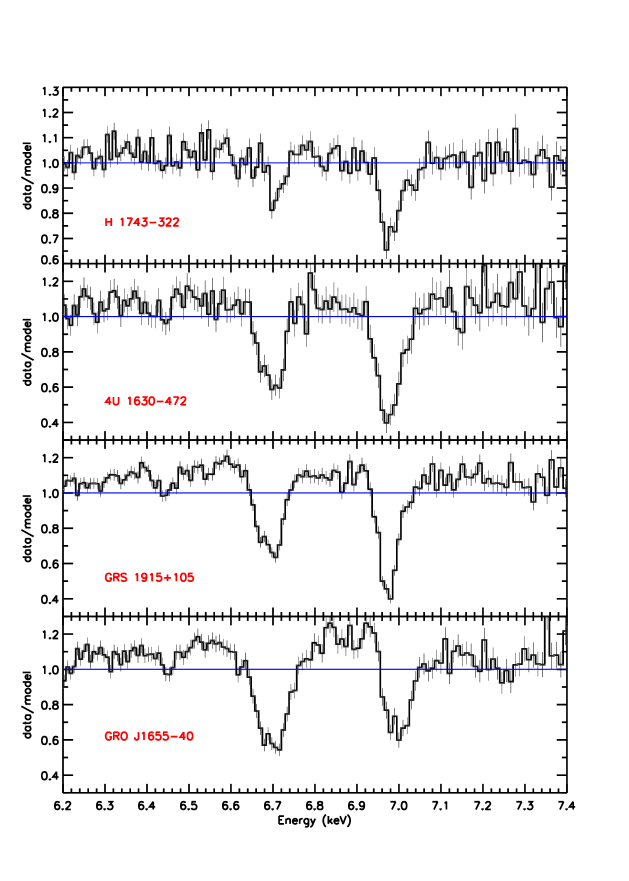
Figure 1.— The first-order spectra of H 1743$-$322, 4U 1630$-$472, GRS 1915$+$105, and GRO J1655$-$40 are each shown as a ratio to the best-fit continuum model, initially ignoring the Fe K band. Each model included disk blackbody and power-law components, with power-law indices constrained via broad-band fits to simultaneous RXTE data, where possible. The He-like Fe XXV and H-like Fe XXVI absorption lines in each spectrum show non-Gaussian structure, indicating contributions from related lines and/or multiple velocity components. Evidence of weak emission redward of the absorption lines is also apparent, especially in GRO J1655$-$40 and GRS 1915$+$105, and suggestive of disk-like P-Cygni profiles.

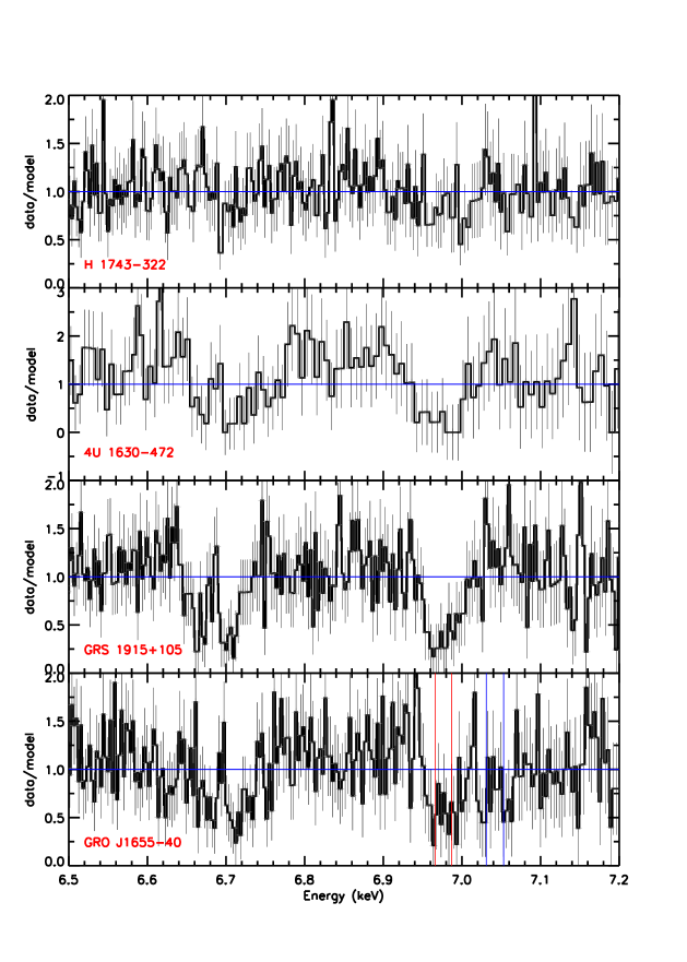
Figure 2.— The third-order spectra of H 1743$-$322, 4U 1630$-$472, GRS 1915$+$105, and GRO J1655$-$40 are each shown as a ratio to a simple continuum, as per the prior figure. Third-order spectra have three times higher resolution than first-order spectra; the resolution of these spectra is only a factor of a few lower than the spectra anticipated from Astro-H. In the most sensitive spectra, the Fe XXV complex is resolved into distinct lines, with the intercombination line seen in absorption (in addition to the resonance line). Especially in GRO J1655$-$40, but also evident in other spectra, the Fe XXVI line is resolved as a doublet - for the first time - owing spin-orbit coupling (analytical theory predicts a separation of just 0.02 keV, as observed). The doublet is evident just below 7.0 keV and just above 7.0 keV in GRO J1655$-$40, clearly indicating a high velocity component. Vertical lines indicate the theoretical separation for the pairs.

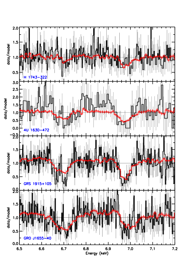
Figure 3.— The first-order data/model ratios of H 1743$-$4322, 4U 1630$-$472, GRS 1915$+$105, and GRO J1655$-$40 (shown in red) are plotted on top of the third-order data/model ratios (shown in black). The individual lines seen in the third-order spectra clearly map onto the structure and asymmetries seen in the more senstiive first-order spectra.

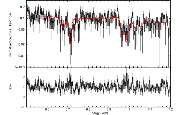
Figure 4.— The third-order spectrum of GRO J1655$-$40, fit with a three-zone model (1655-3a; see Table 3). The Fe XXV complex (6.67-6.70 keV) is clearly resolved, and the second-strongest line is the intercombination line. The Fe XXVI lines are individually resolved, and independent pairs at smaller and larger shifts are evident. The pair at the highest blue shift has an unexpected flux ratio but this is partly accounted for by the inclusion of a third absorption zone; a third zone is also required in fits to the lower-resolution but more sensitive first-order spectrum.

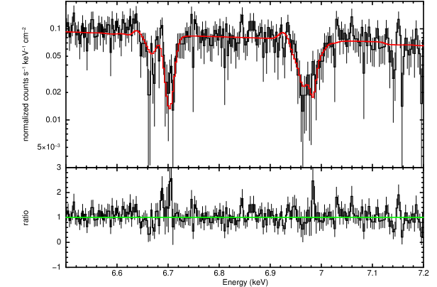
Figure 5.— The third-order spectrum of GRS J1915$+$105, fit with a three-zone model (1915-3a; see Table 4). The Fe XXV complex (6.67-6.70 keV) is clearly resolved, and the second-strongest line is the intercombination line. The Fe XXVI line shows structure, including a tail to the blue indicating a high velocity component.

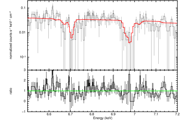
Figure 6.— The third-order spectrum of 4U 1630$-$472, fit with a two-zone model (1630-3a; see Table 5). The spectrum was rebinned for visual clarity, in the plot above. The sensitivity of this spectrum is considerably less than that seen in GRO J1655$-$40 or GRS 1915$+$105, but this spectrum clearly indicates the need for two components in fits to the more sensitive first-order spectrum of 4U 1630$-$472.

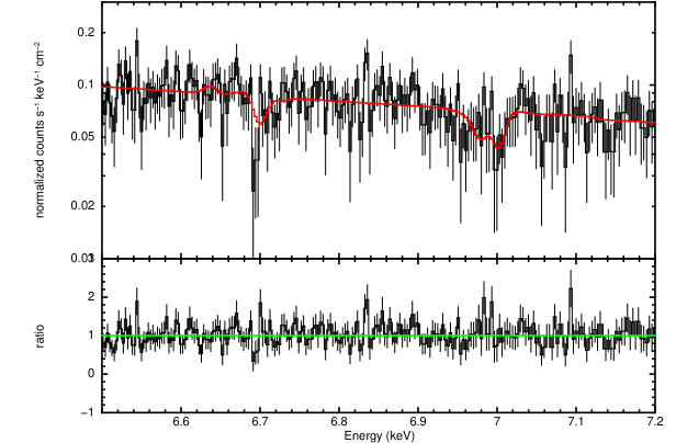
Figure 7.— The third-order spectrum of H 1743$-$322, fit with a two-zone model (1743-3a; see Table 6). The sensitivity of this spectrum is considerably less than that seen in GRO J1655$-$40 or GRS 1915$+$105, but the large blue-shift in the Fe XXVI line and asymmetry in the Fe XXV complex are apparent. This spectrum clearly indicates the need for two components in fits to the more sensitive first-order spectrum of H 1743$-$322.

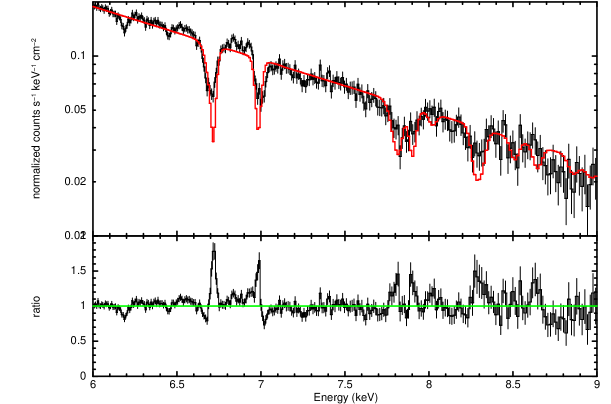
Figure 8.— The first-order spectrum of GRO J1655$-$40 is shown here, fit with the best model for the Fe K band in Miller et al. (2008). Emission components are not included in the model, which is comprised of a single absorption zone. This model was vastly superior to others considered in Miller et al. (2008), though it was not an excellent description of the data. Using the procedures in this paper, the overall fit achieved is markedly worse ($\chi^{2}/\nu=1555/489=3.180$) than the multiple-zone models including corresponding emission, detailed in Table 7 (model 1655-1a gives $\chi^{2}/\nu=624/475=1.315$).

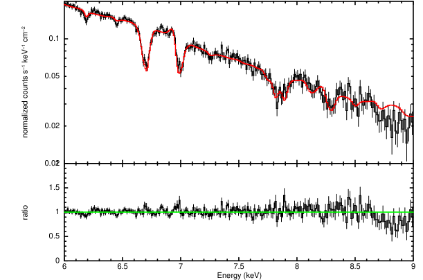
Figure 9.— The first-order spectrum of GRO J1655$-$40 is shown here, fit with model 1655-1a in Table 7. The model includes three absorption zones, and corresponding emission lines from gas with the same properties. Blurring of the emission components by factors commensurate with Keplerian rotation at the photoionization radius is required by the data. The fit is vastly superior to the simple model published in Miller et al. (2008) and shown in the prior figure.

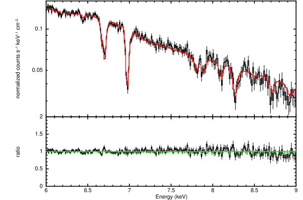
Figure 10.— The first-order spectrum of GRS 1915$+$105 is shown here, fit with model 1915-1a in Table 8. The model includes three absorption zones, and corresponding emission lines from gas with the same properties. Blurring of the emission components by factors commensurate with Keplerian rotation at the photoionization radius is required by the data.

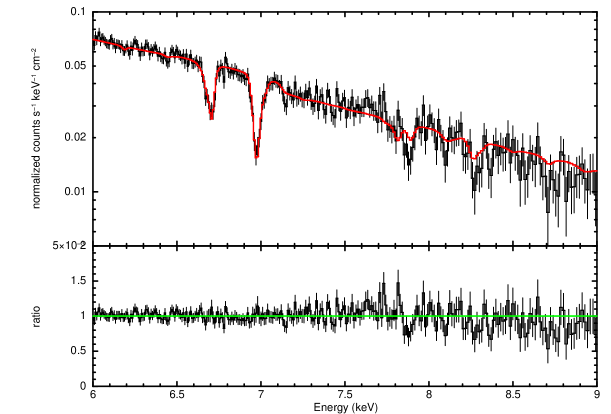
Figure 11.— The first-order spectrum of 4U 1630$-$472 is shown here, fit with model 1630-1a in Table 9. The model includes three absorption zones, and corresponding emission lines from gas with the same properties. Blurring of the emission components by factors commensurate with Keplerian rotation at the photoionization radius is required by the data.

Figure 12.— The first-order spectrum of H 1743$-$322 is shown here, fit with model 1743-1a in Table 10. The model includes two absorption zones, and corresponding emission lines from gas with the same properties. The two-component model is able to fit asymmetries in the absorption lines that cannot be described with a single zone.

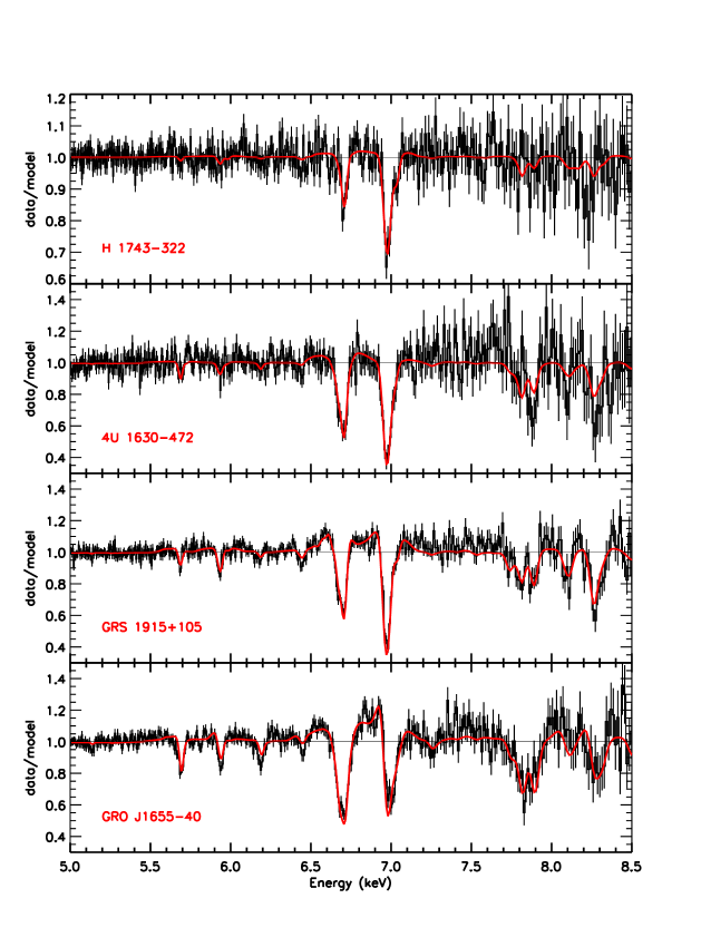
Figure 13.— The first-order spectra of H 1743$-$322, 4U 1630$-$472, GRS 1915$+$105, and GRO J1655$-$40 are each shown as a ratio to the best-fit continuum models from Table 11. To construct each ratio, the photoionized absorption and emission components were removed from the total spectral model. The model with the photoionized components is then plotted through the ratio, to illustrate the relative importance of absorption and emission in the spectra. Evidence of disk-like P-Cygni profiles is strong in GRO J1655$-$40 and GRS 1915$+$105, and tentative in 4U 1630$-$472 and H 1743$-$322.

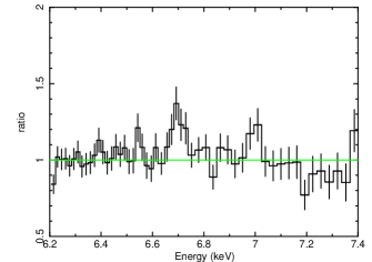
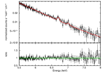
Figure 14.— A sensitive Chandra/HETG observation of GX 339$-$4 in the high/soft state may show evidence of a disk wind seen in emission (see Section 4.9). LEFT: The data/model ratio from a simple disk blackbody plus power-law fit. The ratio shown in this figure contains modest evidence of He-like Fe XXV and H-like Fe XXVI emission lines (6.70 keV and 6.97 keV, respectively). RIGHT: The spectrum of GX 339$-$4, fit with a model including the XSTAR wind emission component used in fits to GRO J1655$-$40 (see Tables 3, 7, 11). The inclusion of the wind component is significant at the $5\sigma$ level of confidence. The spectrum requires the emission component to be blue-shifted by $v=1700\pm 300$ km/s, consistent with a disk wind.

Table 1Sources and Observation Characteristics

Source	Observation	Duration	Start Date	Selected References
		($10^{3}$ s)	(YYYY-MM-DD)
4U 1630$-$472	13715	29.3	2012-01-20	Neilsen et al. 2014
GRO J1655$-$40	5461	65.6	2005-04-01	Miller et al. 2006, 2008; Kallman et al. 2009
H 1743$-$322	3803	46.5	2003-05-01	Miller et al. 2006, 2012
GRS 1915$+$105	7485	47.4	2007-08-14	Ueda et al. 2009, Neilsen & Lee 2009
GX 339$-$4	4571	35.3	2004-10-28	–

Table 2XSTAR Photoionization Grid Input Parameters

Source	Luminosity	kT	log(n)	$v_{turb}$	${\rm A}_{Fe}$	$f=\Omega/4\pi$
	($10^{38}~{}{\rm erg}~{}{\rm s}^{-1}$)	(keV)		${\rm km}~{}{\rm s}^{-1}$
4U 1630$-$472	1.1	1.5	14.0	400	1.0	0.5
GRO J1655$-$40	0.5	1.3	14.0	300	1.0	0.2
H 1743$-$322	2.0	1.2	14.0	400	1.0	0.5
GRS 1915$+$105	8.0	1.9	14.0	400	2.0	0.5

Table 3Fits to the Third Order Spectrum of GRO J1655$-$40

Model	Notes	Zone 1	Zone 2	Zone 3	Continuum	$\chi^{2}/\nu$
Example	3 zones, emis. incl., blurring	${\rm N}_{1}$	${\rm N}_{2}$	${\rm N}_{3}$	kT (keV)	$500/500=1$
		${\rm log}(\xi_{1})$	${\rm log}(\xi_{2})$	${\rm log}(\xi_{3})$	${\rm K}_{disk}$
		$v_{abs,1}/c$	$v_{abs,2}/c$	$v_{abs,3}/c$	$\Gamma$
		$v_{emis,1}/c$	$v_{emis,2}/c$	$v_{emis,3}/c$	${\rm K}_{pow}$
		$\sigma_{emis,1}$	$\sigma_{emis,2}$	$\sigma_{emis,2}$
		${\rm K}_{emis,1}$	${\rm K}_{emis,2}$	${\rm K}_{emis,3}$
1655-3a	3 zones, emis. incl., blurring	$22(4)$	$5^{+15}_{-2}$	$16^{+2}_{-4}$	1.3*	$1135/1098=1.033$
		$4.42(5)$	$4.7_{-0.2}^{+1.3}$	$5.1(1)$	400
		$-1.8(1)$	$-7.5(5)$	$-11.8(5)$	3.5*
		$1.2$	$3.4$	$2.0$	22
		$0.19$	$3^{+4}_{-3}$	$0^{+12}$
		$0.1$	$0.2_{-0.1}^{+3}$	$5(3)$
1655-3b	2 zones, emis. incl., blurring	$46(5)$	$16(5)$	–	1.3*	$1139/1101=1.033$
		$4.8(1)$	$5.5(2)$	–	400(50)
		$-1.8(1)$	$-11.4(5)$	–	3.5*
		$0^{+1.8}$	$0^{+11}$	–	84(3)
		$0.2_{-0.1}$	$0.03(1)$	–
		$0.15(5)$	$5(2)$	–
1655-3c	2 zones, emis. incl., no blurring	$46$	$7.5$	–	1.3*	$1144/1103=1.197$
		$4.8$	$4.9$	–	309
		$-1.6$	$-11.5$	–	3.5*
		$0$	$0$	–	37
		–	–	–
		0.1*	2.7	–
1655-3d	1 zone, emis. incl., no blurring	$13$	$--$	–	1.3*	$1172/1109=1.058$
		$4.4$	–	–	340
		$-1.9$	–	–	3.5*
		$0$	–	–	87
		–	–	–
		0.1*	–	–

Table 4Fits to the Third Order Spectrum of GRS 1915$+$105

Model	Notes	Zone 1	Zone 2	Zone 3	Continuum	$\chi^{2}/\nu$
Example	3 zones, emis. incl., blurring	${\rm N}_{1}$	${\rm N}_{2}$	${\rm N}_{3}$	kT (keV)	$500/500=1$
		${\rm log}(\xi_{1})$	${\rm log}(\xi_{2})$	${\rm log}(\xi_{3})$	${\rm K}_{disk}$
		$v_{abs,1}/c$	$v_{abs,2}/c$	$v_{abs,3}/c$	$\Gamma$
		$v_{emis,1}/c$	$v_{emis,2}/c$	$v_{emis,3}/c$	${\rm K}_{pow}$
		$\sigma_{emis,1}$	$\sigma_{emis,2}$	$\sigma_{emis,2}$
		${\rm K}_{emis,1}$	${\rm K}_{emis,2}$	${\rm K}_{emis,3}$
1915-3a	3 zones, emis. incl., blurring	$40_{-10}^{+20}$	$20_{-10}^{+10}$	$3_{-2}^{+12}$	1.9(1)	$1059/1094=0.967$
		$3.95(5)$	$6.0_{-0.5}$	$4.27(5)$	53(1)x
		$-0.3_{-0.6}^{+0.3}$	$-0.3^{+0.3}$	$-4(1)$	3.0*
		$0.0^{+0.3}$	$4(2)$	$0.0^{+0.2}$	$0^{+4}$
		$0.2_{-0.1}$	$0.04(4)$	$0.00^{+0.03}$
		$0.10^{+0.03}$	$0.1^{+0.2}$	$0.4(2)$
1915-3b	2 zones, emis. incl., blurring	$50_{-20}^{+10}$	$5_{-2}^{+5}$	–	1.9(1)	$1067/1101=0.969$
		$3.94(7)$	$4.4(2)$	–	53(1)
		$-0.4_{-0.1}^{+0.4}$	$-4(1)$	–	3.0*
		$0^{+2}$	$0.0^{+0.6}$	–	$0^{+4}$
		$0.2_{-0.05}$	$0.1^{+0.4}$	–
		$0.13(3)$	$0.7(3)$	–
1915-3c	2 zones, emis incl., no blurring	$46$	$7.5$	–	1.9(1)	$1111/1103=1.197$
		$4.8$	$4.68$	–	53
		$-1.6$	$-3.3$	–	3.0*
		$0$	$0$	–	0.0
		–	–	–
		0.1	0.1	–
1915-3d	2 zones, no emis., no blurring	$6.4$	$12.5$	–	1.9	$1093/1107=0.988$
		$3.89$	$4.55$	–	54
		$-0.4$	$-2.9$	–	3.0*
		–	–	–	0
		–	–	–
		–	–	–
1915-3e	1 zone, no emis., no blurring	$10.6$	$--$	–	1.9	$1101/1110=0.992$
		$3.9$	–	–	54
		$-0.7$	–	–	3.0*
		–	–	–	0
		–	–	–
		–	–	–

Table 5Fits to the Third Order Spectrum of 4U 1630$-$472

Model	Notes	Zone 1	Zone 2	Zone 3	Continuum	$\chi^{2}/\nu$
Example	3 zones, emis. incl., Gauss. blurring	${\rm N}_{1}$	${\rm N}_{2}$	${\rm N}_{3}$	kT (keV)	$500/500=1$
		${\rm log}(\xi_{1})$	${\rm log}(\xi_{2})$	${\rm log}(\xi_{3})$	${\rm K}_{disk}$
		$v_{abs,1}/c$	$v_{abs,2}/c$	$v_{abs,3}/c$	$\Gamma$
		$v_{emis,1}/c$	$v_{emis,2}/c$	$v_{emis,3}/c$	${\rm K}_{pow}$
		$\sigma_{emis,1}$	$\sigma_{emis,2}$	$\sigma_{emis,2}$
		${\rm K}_{emis,1}$	${\rm K}_{emis,2}$	${\rm K}_{emis,3}$
1630-3a	2 zones, emis. incl., Gauss. blurring	$50^{+10}_{-20}$	$2^{+1}_{-1}$	–	1.45(5)	$1061/1101=0.963$
		$4.3(2)$	$4.2(2)$	–	$110(20)$
		$-1.0(3)$	$-7.0_{-2.0}^{+3.0}$	–	–
		$0.2^{+0.2}_{-0.2}$	$0.7^{0.1}_{-0.7}$	–	–
		$0.16(4)$	$0.02^{+0.01}_{-0.02}$	–
		$0.10^{+0.04}$	$0.1(1)$	–
1630-3b	2 zones, emis. incl., no blurring	$60$	$3$	–	1.45	$1077/1103=0.963$
		$4.7$	$3.5$	–	105
		$-0.7$	$-8.0$	–	–
		0.0	3.5	–	–
		–	–	–
		$0.1$	$0.1$	–
1630-3c	1 zones, emis. incl., no blurring	$60$	–	–	1.48	$1088/1108=0.963$
		$4.6$	–	–	92
		$-0.9$	–	–	–
		0.0	3.5	–	–
		–	–	–
		$0.1$	–	–

Table 6Fits to the Third Order Spectrum of H 1743$-$322

Model	Notes	Zone 1	Zone 2	Zone 3	Continuum	$\chi^{2}/\nu$
Example	3 zones, emis. incl., Gauss. blurring	${\rm N}_{1}$	${\rm N}_{2}$	${\rm N}_{3}$	kT (keV)	$500/500=1$
		${\rm log}(\xi_{1})$	${\rm log}(\xi_{2})$	${\rm log}(\xi_{3})$	${\rm K}_{disk}$
		$v_{abs,1}/c$	$v_{abs,2}/c$	$v_{abs,3}/c$	$\Gamma$
		$v_{emis,1}/c$	$v_{emis,2}/c$	$v_{emis,3}/c$	${\rm K}_{pow}$
		$\sigma_{emis,1}$	$\sigma_{emis,2}$	$\sigma_{emis,2}$
		${\rm K}_{emis,1}$	${\rm K}_{emis,2}$	${\rm K}_{emis,3}$
1743-3a	2 zones, emis. incl., Gauss. blurring	$8_{-5}$	$24^{+6}_{-16}$	–	0.8(1)	$1112/1100=1.011$
		$4.7(2)$	$6_{-1}$	–	$6000(3000)$
		$0.0^{+0.1}$	$-4(1)$	2.4*	–
		$0.0^{+0.1}$	$0.0^{+0.1}$	5.6(5)	–
		$0.0^{+0.1}$	$0.02^{+0.01}_{-0.02}$	–
		$2.2_{-1.4}^{+1.0}$	$2.2_{-1.6}^{+7.8}$	–
1743-3b	2 zones, emis. incl., no blurring	$8.3$	$25$	–	0.81	$1112/1102=1.009$
		$4.7$	$6.0$	–	5900
		$0.0$	$-4.3$	2.4*	–
		0.0	0.01	–	5.7
		–	–	–
		$2.3$	$0.1$	–
1743-3c	2 zones, no emis., no blurring	$1.4$	$25.0$	–	0.81	$1117/1106=1.010$
		$4.5$	$6.0$	–	5500
		$0.0$	$-4.3$	–	2.4*
		–	–	–	5.6
		–	–	–
		–	–	–
1743-3d	1 zones, no emis., no blurring	$15.3$	–	–	0.83	$1124/1109=1.014$
		$5.4$	–	–	5100
		$-3.9$	–	–	2.4*
		–	–	–	5.6
		–	–	–
		–	–	–

Table 7Fits to the First Order Spectrum of GRO J1655$-$40

Model	Notes	Zone 1	Zone 2	Zone 3	Continuum	$\chi^{2}/\nu$
Example	3 zones, emis. incl., Gauss. blurring	${\rm N}_{1}$	${\rm N}_{2}$	${\rm N}_{3}$	kT (keV)	$500/500=1$
		${\rm log}(\xi_{1})$	${\rm log}(\xi_{2})$	${\rm log}(\xi_{3})$	${\rm K}_{disk}$
		$v_{abs,1}/c$	$v_{abs,2}/c$	$v_{abs,3}/c$	$\Gamma$
		$v_{emis,1}/c$	$v_{emis,2}/c$	$v_{emis,3}/c$	${\rm K}_{pow}$
		$\sigma_{emis,1}$	$\sigma_{emis,2}$	$\sigma_{emis,2}$
		${\rm K}_{emis,1}$	${\rm K}_{emis,2}$	${\rm K}_{emis,3}$
1655-1a	3 zones, emis. incl., Gauss. blurring	$59^{+1}_{-3}$	$8.2^{+0.5}_{-1.2}$	$4.2^{+0.4}_{-0.7}$	1.22(1)	$634/477=1.329$
		$4.72(4)$	$4.53(3)$	$4.95(5)$	930(30)
		$-1.5(1)$	$-6.4(4)$	$-11.8*$	3.5*
		$0^{+0.1}$	$0.0^{+0.1}$	$0.0^{+0.1}$	$4_{-3}^{+10}$
		$0.25(5)$	$0.22(4)$	$0.018(4)$	$0.12^{+0.11}_{-0.04}$
		$0.10^{0.01}$	$2.5(5)$	$10_{-2}$	$0.5^{+0.6}_{-0.4}$
1655-1b	3 zones, emis. incl., no blurring	$58$	$8.2$	$3.2$	1.25	$928/480=1.934$
		$4.7$	$5.1$	$4.9$	800
		$-1.3$	$-6.7$	$-11.8*$	3.5*
		$0$	$0.0$	$0$	0
		–	–	–	0.12
		$0.1$	$5.0$	$0.1$	0.5
1655-1c	3 zones, no emis., no blurring	$19$	$0.4$	$0.3$	1.27	$963.0/484=1.990$
		$4.3$	$4.7$	$3.3$	741
		$-2.3$	$-8.4$	$-11.8*$	3.5*
		–	–	–	0
		–	–	–	0.12
		–	–	–	1.8
1655-1d	2 zones, emis. incl., Gauss. blurring	$54$	–	$4.4$	1.22(1)	$732/481=1.521$
		$4.6$	–	$4.7$	880
		$-2.2$	–	$-11.8*$	3.5*
		$0$	–	$0$	0
		$0.24$	–	$0.02$	0.09
		$0.25$	–	$3.7$	0.05
1655-1e	2 zones, emis. incl., no blurring	$56$	–	$0.8$	1.25(1)	$732/481=1.521$
		$4.7$	–	$5.3$	810
		$-1.7$	–	$-11.8*$	3.5*
		$0$	–	$0$	0
		–	–	–	0.12
		$0.1$	–	$6.2$	2.0
1655-1f	2 zones, no emis., no blurring	$35$	–	$3.8$	1.27	$995/486=2.043$
		$4.5$	–	$4.8$	740
		$-2.7$	–	$-11.8*$	3.5*
		–	–	–	0.001
		–	–	–	0.3
		–	–	–	3.7

Table 8Fits to the First Order Spectrum of GRS 1915$+$105

Model	Notes	Zone 1	Zone 2	Zone 3	Continuum	$\chi^{2}/\nu$
Example	3 zones, emis. incl., Gauss. blurring	${\rm N}_{1}$	${\rm N}_{2}$	${\rm N}_{3}$	kT (keV)	$500/500=1$
		${\rm log}(\xi_{1})$	${\rm log}(\xi_{2})$	${\rm log}(\xi_{3})$	${\rm K}_{disk}$
		$v_{abs,1}/c$	$v_{abs,2}/c$	$v_{abs,3}/c$	$\Gamma$
		$v_{emis,1}/c$	$v_{emis,2}/c$	$v_{emis,3}/c$	${\rm K}_{pow}$
		$\sigma_{emis,1}$	$\sigma_{emis,2}$	$\sigma_{emis,2}$
		${\rm K}_{emis,1}$	${\rm K}_{emis,2}$	${\rm K}_{emis,3}$
1915-1a	3 zones, emis. incl., Gauss. blurring	$42(4)$	$60_{-10}$	$0.7_{-0.2}^{+0.1}$	1.90(1)	$757/476=1.591$
		$3.76(3)$	$5.04^{+0.06}_{-0.2}$	$3.82(4)$	68(2)
		$-0.5(1)$	$-1.7(3)$	$-7.2(6)$	3.0*
		$0.0^{+0.1}$	$0.0^{+0.1}$	$0.0^{+0.1}$	$0.0^{+0.2}$
		$0.29_{-0.01}$	$0.02(1)$	$0.07(1)$	$0.11^{+0.05}_{-0.03}$
		$0.10^{+0.02}$	$0.28^{+0.06}_{-0.09}$	$1.7^{+0.4}_{-0.2}$	$1.2(4)$
1915-1b	3 zones, emis. incl., no blurring	$47$	$60$	$0.6$	1.92	$1003/479=2.095$
		$3.9$	$4.5$	$6.0$	66
		$0.0$	$-0.9$	$-65$	3.0*
		$0.0$	$0.0$	$0.0$	0.0
		–	–	–	0.3
		$0.10$	$1.2$	$20$	6.6
1915-1c	3 zones, no emis., no blurring	$18$	$0.3$	$0.3$	1.94	$1040/482=2.153$
		$4.0$	$3.2$	$6.0$	63
		$-1.0$	$-19$	$-99$	3.0*
		–	–	–	0.0
		–	–	–	0.3
		–	–	–	7.2
1915-1d	2 zones, emis. incl., Gauss. blurring	$44$	60	–	1.91	$829/481=1.724$
		$4.0$	5.3	–	67
		$-0.6$	$-2.3$	–	3.0*
		$0.0$	$0.0$	–	0
		$0.10$	$0.02$	–	0.27
		$0.10$	$0.8$	–	5.2
1915-1e	2 zones, emis. incl., no blurring	$43$	49	–	1.92	$1007/483=2.084$
		$3.9$	4.4	–	66
		$0.0$	$-1.0$	–	3.0*
		$0.0$	$0.0$	–	0
		–	–	–	0.3
		$0.1$	$0.1$	–	7.0
1915-1f	2 zones, no emis., no blurring	$4.0$	41	–	1.92	$1203/486=2.475$
		$3.9$	4.8	–	66
		$0.0$	$-1.6$	–	3.0*
		–	–	–	0
		–	–	–	0.3
		–	–	–	7.0

Table 9Fits to the First Order Spectrum of 4U 1630$-$472

Model	Notes	Zone 1	Zone 2	Zone 3	Continuum	$\chi^{2}/\nu$
Example	3 zones, emis. incl., Gauss. blurring	${\rm N}_{1}$	${\rm N}_{2}$	${\rm N}_{3}$	kT (keV)	$500/500=1$
		${\rm log}(\xi_{1})$	${\rm log}(\xi_{2})$	${\rm log}(\xi_{3})$	${\rm K}_{disk}$
		$v_{abs,1}/c$	$v_{abs,2}/c$	$v_{abs,3}/c$	$\Gamma$
		$v_{emis,1}/c$	$v_{emis,2}/c$	$v_{emis,3}/c$	${\rm K}_{pow}$
		$\sigma_{emis,1}$	$\sigma_{emis,2}$	$\sigma_{emis,2}$
		${\rm K}_{emis,1}$	${\rm K}_{emis,2}$	${\rm K}_{emis,3}$
1630-1a	2 zones, emis. incl., Gauss. blurring	$22(2)$	$7^{+3}_{-2}$	–	1.49(1)	$518/481=1.074$
		$4.14(2)$	$4.6^{+0.3}_{-0.1}$	–	$126(5)$
		$-0.7_{-0.3}^{+0.4}$	$-6.0(2)$	–	–
		$0.0^{+0.1}$	$0.0^{+0.1}$	–	–
		$0.29_{-0.12}^{+0.03}$	$0.0^{+0.05}$	–	$0.20_{-0.08}$
		$0.11^{+0.04}$	$0.3(2)$	–	$0.9(4)$
1630-1b	2 zones, emis. incl., no blurring	$8.2$	$31.0$	–	1.49	$573/483=1.185$
		$4.0$	$4.6$	–	$127$
		$0$	$0$	–	–
		$0.0$	$0.0$	–	–
		–	–	–	0.2
		$0.1$	$0.1$	–	1.2
1630-1c	2 zones, no emis., no blurring	$6.6$	$20.2$	–	1.51	$528/485=1.088$
		$4.1$	$4.5$	–	$119$
		$0.0$	$0.0$	–	–
		–	–	–	–
		–	–	–	0.2
		–	–	–	1.4
1630-1d	1 zone, no emis., no blurring	$22.2$	–	–	1.49	$529/488=1.084$
		$4.17$	–	–	$126$
		$-1.2$	–	–	–
		–	–	–	–
		–	–	–
		–	–	–

Table 10Fits to the First Order Spectrum of H 1743$-$322

Model	Notes	Zone 1	Zone 2	Zone 3	Continuum	$\chi^{2}/\nu$
Example	3 zones, emis. incl., Gauss. blurring	${\rm N}_{1}$	${\rm N}_{2}$	${\rm N}_{3}$	kT (keV)	$500/500=1$
		${\rm log}(\xi_{1})$	${\rm log}(\xi_{2})$	${\rm log}(\xi_{3})$	${\rm K}_{disk}$
		$v_{abs,1}/c$	$v_{abs,2}/c$	$v_{abs,3}/c$	$\Gamma$
		$v_{emis,1}/c$	$v_{emis,2}/c$	$v_{emis,3}/c$	${\rm K}_{pow}$
		$\sigma_{emis,1}$	$\sigma_{emis,2}$	$\sigma_{emis,2}$
		${\rm K}_{emis,1}$	${\rm K}_{emis,2}$	${\rm K}_{emis,3}$
1743-1a	2 zones, emis. incl., Gauss. blurring	$6.1(6)$	$14_{-8}^{+3}$	–	1.10(1)	$723/478=1.513$
		$4.57(3)$	$6.0_{-0.5}$	–	$1090(50)$
		$-1.0(3)$	$-8.6(9)$	–	2.4*
		$50(20)$	$5^{+15}$	–	2.45(8)
		$0.08_{-0.08}^{+0.08}$	$0.20_{-0.01}$	–	$0.2_{-0.02}$
		$0.5_{-0.4}^{+0.7}$	$10_{-2}$	–	2.3(3)
1743-1b	2 zones, emis. incl., no blurring	$5.7$	$13.2$	–	1.10	$728/480=1.518$
		$4.58$	$6.0$	–	$1195$
		$-1.0(3)$	$-8.5$	–	2.4*
		$0.0$	$0.0$	–	2.8
		–	–	–	0.2
		$0.12$	$0.68$	–	2.1
1743-1c	2 zones, no emis., no blurring	$5.7$	$13.2$	–	1.10	$739/484=1.527$
		$4.58$	$6.0$	–	$1215$
		$-1.0$	$-8.5$	–	2.4*
		–	–	–	2.8
		–	–	–	0.2
		–	–	–	2.1
1743-1d	1 zones, no emis., no blurring	$6.0$	–	–	1.09	$742/487=1.579$
		$4.59$	–	–	$1225$
		$-1.3$	–	–	2.4*
		–	–	–	2.8
		–	–	–	0.2
		–	–	–	2.3

Table 11Radius-focused Fits to First Order Spectra

Model	Notes	Zone 1	Zone 2	Zone 3	Continuum	$\chi^{2}/\nu$
Example	3 zones, emis. incl., Gauss. blurring	${\rm N}_{1}$	${\rm N}_{2}$	${\rm N}_{3}$	kT (keV)	$500/500=1$
		${\rm log}(\xi_{1})$	${\rm log}(\xi_{2})$	${\rm log}(\xi_{3})$	${\rm K}_{disk}$
		$v_{abs,1}/c$	$v_{abs,2}/c$	$v_{abs,3}/c$	$\Gamma$
		$R_{in,1}$	$R_{in,2}$	$R_{in,3}$	${\rm K}_{pow}$
		$\theta_{1}$	$\theta_{2}$	$\theta_{3}$	$\sigma$ (keV)
		${\rm K}_{emis,1}$	${\rm K}_{emis,2}$	${\rm K}_{emis,3}$	$K_{gauss}$
1655-r1	3 zones, emis. incl., linked blurring	$49(2)$	$7.6(8)$	$8^{+2}_{-1}$	$1.22(1)$	$710/477=1.490$
		$4.59(3)$	$4.65(4)$	$5.0^{+0.3}_{-0.1}$	$940(10)$
		$-2.2(1)$	$-7.8(5)$	$-11.8*$	$3.5*$
		$1600^{+300}_{-100}$	$1600_{-100}^{+300}$	$1600^{+300}_{-100}$	$0.7^{+1.5}_{-0.7}$
		$70-85$	$70-85$	$70-85$	$0.12(2)$
		$0.10^{+0.05}$	$2.0(7)$	$10_{-1}$	$2.4(4)$
1655-r2	3 zones, emis. incl., indep. blurring	$55(3)$	$8.3_{-0.5}^{+1.7}$	$4.7(7)$	$1.22(1)$	$671/475=1.414$
		$4.67(5)$	$4.62(2)$	$4.95(5)$	$920(20)$
		$-2.0(2)$	$-7.0(5)$	$-11.8*$	$3.5*$
		$500^{+400}$	$1100^{+200}_{-200}$	$10,000_{-1000}$	$0.0^{+0.5}$
		$70^{+3}$	$70^{+3}$	$70^{+3}$	$0.12(2)$
		$0.10^{+0.01}$	$2.5(5)$	$10_{-1}$	$2.0(4)$
1915-r1	3 zones, emis. incl., linked blurring	$40(7)$	$4(1)$	$60_{-30}$	$1.90(1)$	$793/477=1.662$
		$4.10(5)$	$3.78(5)$	$5.9^{+0.1}_{-0.6}$	$68(2)$
		$-1.0(1)$	$-0.5(5)$	$-9.4(2)$	$3.0*$
		$2400_{-400}^{+600}$	$2400_{-400}^{+600}$	$2400_{-400}^{+600}$	$0.0^{+0.1}$
		$60-80$	$60-80$	$60-80$	$0.14(3)$
		$0.10^{+0.02}$	$2.0(2)$	$2.1(3)$	$3.0(5)$
1915-r2	3 zones, emis. incl., indep. blurring	$40^{+1}_{-5}$	$4.2(5)$	$60_{-3}$	$1.90(1)$	$787/475=1.646$
		$4.10(5)$	$3.8(1)$	$5.9^{+0.1}_{-0.5}$	$68(2)$
		$-1.0(1)$	$-0.5(5)$	$-9.4(2)$	$3.0*$
		$1200_{-200}^{+600}$	$5500_{-700}^{+1000}$	$2400_{-400}^{+600}$	$0.0^{+0.1}$
		$60-80$	$60-80$	$60-80$	$0.14(3)$
		$0.10^{+0.03}$	$2.0(2)$	$2.1(3)$	$2.6(6)$
1630-r1	2 zones, emis. incl., linked blurring	$21^{+2}_{-3}$	$5.0^{+3}_{-2}$	–	$1.48(2)$	$519/481=1.079$
		$4.12(2)$	$4.6(2)$	–	$130(4)$
		$-0.8(3)$	$-6(2)$	–	–
		$800^{+500}_{-200}$	$800^{+500}_{-200}$	–	–
		$65-80$	$65-80$	–	0.17(3)
		$0.10^{+0.05}$	$0.1^{+2}$	–	0.9(4)
1743-r1	2 zones, emis. incl., linked blurring	$6.1(6)$	$14^{+2}_{-9}$	–	$1.09(1)$	$725/482=1.509$
		$4.57(3)$	$6_{-1}$	–	$1250(80)$
		$-1.0(3)$	$-8.7(9)$	–	2.4*
		$1100^{+1100}_{-300}$	$1100^{+1100}_{-300}$	2.8(1)	–
		$60-80$	$60-80$	–	$0.20_{-0.03}$
		$0.7(6)$	$2_{-1}^{+2}$	–	$2.1(4)$

Table 12Wind Launching and Outflow Parameters

Source, zone	$L_{rad}/L_{Edd.}$	$\dot{M}_{wind}$	$\dot{M}_{wind,Edd.}$	$L_{wind}$	$L_{wind}/L_{edd}$	$L_{wind}/L_{rad}$	$r_{phot.}$	$r_{blur}$
		($10^{18}$ g/s)		($10^{34}$ erg/s)	($10^{-4}$)	($10^{-3}$)	(GM/c2)	(GM/c2)
1630-r1, zone 1	0.09	3(1)	0.2(1)	0.07(5)	0.006(4)	$0.006(5)$	$6100\pm 2200$	$800^{+500}_{-200}$
1630-r1, zone 2	0.09	6(3)	0.4(2)	9(6)	0.7(5)	$0.8(6)$	$3300\pm 1600$	$800^{+500}_{-200}$
1743-r1, zone 1	0.15	2.1(8)	0.14(6)	0.09(6)	0.007(4)	$0.005(4)$	$4900\pm 1700$	$1100^{+1100}_{-300}$
1743-r1, zone 2	0.15	1.2(6)	0.08(4)	4(2)	0.3(2)	$0.2(1)$	$1300\pm 900$	$1000^{+1100}_{-300}$
1655-r2, zone 1	0.06	0.32(8)	0.032(8)	0.06(2)	0.006(2)	$0.01(7)$	$3100\pm 600$	$500^{+400}$
1655-r2, zone 2	0.06	1.3(3)	0.13(3)	2.8(8)	0.32(8)	$0.6(3)$	$3300\pm 600$	$1100\pm 200$
1655-r2, zone 3	0.06	1.0(3)	0.1(3)	6(2)	0.006(2)	$1.2(7)$	$2300\pm 400$	$10000_{-1000}$
1915-r2, zone 1	0.61	24(6)	1.7(5)	1.1(3)	0.08(2)	$0.013(7)$	$17,000\pm 3000$	$1200^{+600}_{-200}$
1915-r2, zone 2	0.61	26(22)	2(2)	$0.4_{-0.4}^{0.5}$	0.03(3)	$0.005(5)$	$23,000\pm 6000$	$5500^{+1000}_{-700}$
1915-r2, zone 3	0.61	5(2)	0.3(1)	19(7)	1.5(6)	$0.2(1)$	$2400\pm 1300$	$2400^{+600}_{-400}$

References

- (1)
- (2) Arnaud, K., 1996, Astronomical Data Analysis Software and Systems V, ASP Converence Series, eds. G. H. Jacoby and J. Barnes, 101, 17
- (3)
- (4) Begelman, M., & Armitage, P., 2014, ApJ, 782, L18
- (5)
- (6) Begelman, M. C., McKee, C. F., & Shields, G. A., 1983, ApJ, 271, 70
- (7)
- (8) Blustin, A. J., Page, M. J., Fuerst, S. V., Branduardi-Raymont, G., Ashton, C. E., 2005, A&A, 431, 111
- (9)
- (10) Brandt, W. N., & Schulz, N. S., 2000, ApJ, 544, L123
- (11)
- (12) Brenneman, L. W., & Reynolds, C. S., 2006, ApJ, 652, 1028
- (13)
- (14) Cash, W., 1979, ApJ, 228, 939
- (15)
- (16) Calvet, N., Hartmann, L., & Kenyon, S. J., 1993, ApJ, 402, 623
- (17)
- (18) Churazov, E., Gilfanov, M., Forman, W., Jones, C., 1996, ApJ, 471, 673
- (19)
- (20) Crenshaw, D. M., & Kraemer, S. B., 2012, ApJ, 753, 75
- (21)
- (22) Diaz-Trigo, M., Miller-Jones, J. C. A., Migliari, S., Broderick, J., Tzioumis, T., 2013, Nature, 504, 260
- (23)
- (24) Dauser, T., Garcia, J., Wilms, J., et al., 2013, MNRAS, 430, 1694
- (25)
- (26) Dorodnitsyn, A. V., & Kallman, T., 2009, ApJ, 703, 1797
- (27)
- (28) Dorodnitsyn, A. V., 2010, MNRAS, 406, 1060
- (29)
- (30) Esin, A. A., McClintock, J. E., Narayan, R., 1997, ApJ, 489, 865
- (31)
- (32) Fabian, A. C., Rees, M. J., Stella, L., White, N. E., 1989, MNRAS, 238, 729
- (33)
- (34) Ferland, G. J., Korsta, K. T., Verner, D. A., Ferguson, J. W., Kingdon, J. B., Verner, E. M., 1998, PASP, 110, 761
- (35)
- (36) Fragos, T., & McClintock, J. E., 2015, ApJ, 800, 17
- (37)
- (38) Gallo, E., Corbel, S., Fender, R. P., Maccarone, T. J., Tziomis, A. K., 2004, MNRAD, 347, L52
- (39)
- (40) Garcia, J. A., Steiner, J. F., McClintock, J. E., Remillard, R. A., Grinberg, V., Dauser, T., 2015, ApJ, subm., arxiv:1505.03607
- (41)
- (42) Giustini, M., & Proga, D., 2012, ApJ, 758, 70
- (43)
- (44) Grevesse, N., Noels, A., Sauval, A. J., 1996, ASP Conf. Ser. 99, Cosmic Abundances, ed. S. S. Holt & G. Sonneborn (San Francisco, CA: ASP), 117
- (45)
- (46) Higginbottom, N., & Proga, D., 2015, ApJ, in press, arxiv:1504.03328
- (47)
- (48) Hopkins, P., & Elvis, M., 2010, MNRAS, 401, 7
- (49)
- (50) Juett, A. M., Schulz, N. S., Chakrabarty, D., Corczyca, T. W., 2006, ApJ, 648, 1066
- (51)
- (52) Kaastra, J., et al., on behalf of the Astro-H Science Working Group, an Astro-H White Paper, 2014, arxiv:1412.1171
- (53)
- (54) Kallman, T. R., & Bautista, M. A., 2001, ApJS, 133, 221
- (55)
- (56) Kallman, T. R., Bautista, M. A., Goriely, S., Mendoza, C., Miller, J. M., Palmieri, P., Quinet, P., Raymond, J., 2009, ApJ, 701, 865
- (57)
- (58) Kaspi, S., et al., 2002, ApJ, 574, 643
- (59)
- (60) King, A. L., Miller, J. M., Raymond, J., 2012, ApJ, 746, 2
- (61)
- (62) King, A. L., Miller, J. M., Raymond, J., Fabian, A. C., Reynolds, C. S., Kallman, T. R., Maitra, D., Cackett, E. M., Rupen, M. P., 2012, ApJ, 746, L20
- (63)
- (64) King, A. L., Miller, J. M., Raymond, J., Fabian, A. C., Reynolds, C. S., Gultekin, K., Cackett, E. M., Allen, S. W., Proga, D., Kallman, T. R., 2013, ApJ, 762, 103
- (65)
- (66) King, A. L., et al., 2014, ApJ, 784, L2
- (67)
- (68) Kriss, G. A., Krolik, J. H., Otani, C., Espey, B. R., Turner, T. J., Kii, T., Tsetanov, Z., Takahashi, T., Davidsen, A. F., Tashiro, M., Zheng, W., Murakami, S., Petre, R., Mihara, T., 1996, ApJ, 467, 629
- (69)
- (70) Krongold, Y., Nicastro, F., Elvis, M., Brickhouse, N., Binette, L., Mathur, S., Jimenez-Bailon, E., 2007, ApJ, 659, 1022
- (71)
- (72) Kubota, A., Dotani, T., Cottam, J., Kotani, T., Done, C., Ueda, Y., Fabian, A. C., Yasuda, T., Takahashi, H., Fukuzawa, Y., Yamaoka, K., Makishima, K., Yamada, S., Kohmura, T., Angelini, L., 2007, PASJ, 59, 185
- (73)
- (74) Lee, J. C., Ogle, P. M., Canizares, C. R., Marshall, H. L., Schulz, N. S., Morales, R., Fabian, A. C., Iwasawa, K., 2001, ApJ, 554, L13
- (75)
- (76) Lee, J. C., Reynolds, C. S., Remillard, R., Schulz, N. S., Blackman, E. G., Fabian, A. C., 2002, ApJ, 567, 1102
- (77)
- (78) Madej, O. K., Jonker, P. G., Diaz Trigo, M., Miskovicova, I., 2014, MNRAS, 438, 145
- (79)
- (80) Miller, J. M., Raymond, J., Fabian, A., Steeghs, D., Homan, J., Reynolds, C., van der Klis, M., Wijnands, R., 2006, Nature, 441, 953
- (81)
- (82) Miller, J. M., Raymond, J., Homan, J., Fabian, A. C., Steeghs, D., Wijnands, R., Rupen, M., Charles, P., van der Klis, M., Lewin, W. H. G., 2006b, ApJ, 646, 394
- (83)
- (84) Miller, J. M., Raymond, J., Reynolds, C. S., Fabian, A. C., Kallman, T. R., Homan, J., 2008, ApJ, 680, 1359
- (85)
- (86) Miller, J. M., Reynolds, C. S., Fabian, A. C., Miniutti, G., Gallo, L. C., 2009, ApJ, 697, 900
- (87)
- (88) Miller, J. M., Maitra, D., Cackett, E., Bhattacharyya, S., Strohmayer, T. E., 2011, ApJ, 731, L7
- (89)
- (90) Miller, J. M., Raymond, J., Fabian, A. C., Reynolds, C. S., King, A. L., Kallman, T. R., Cackett, E. M., van der Klis, M., Steeghs, D. T. H., 2012, ApJ, 759, L6
- (91)
- (92) Miller, J. M., Raymond, J., Kallman, T. R., Maitra, D., Fabian, A. C., Proga, D., Reynolds, C. S., Reynolds, M. T., Degenaar, N., King, A. L., Cackett, E. M., Kennea, J. A., Beardmore, A., 2014, ApJ, 788, 53
- (93)
- (94) Miller, J. M., Mineshige, S., Kubota, A., Yamada, S., Aharonian, F., Done, C., Kawai, N., Hayashida, K., Reis, R., Mizuno, T., Noda, H., Ueda, Y., Shidatsu, M., for the Astro-H Science Working Group, an Astro-H White Paper, 2014, arxiv:1412.1173
- (95)
- (96) Mitsuda, K., Inoue, H., Koyama, K., Makishima, K., Matsuoka, M., Ogawara, Y., Suzuki, K., Tanaka, Y., Shibazaki, N., Hirano, T., 1984, PASJ, 37, 741
- (97)
- (98) Nardini, E., et al., 2015, Science, 347, 860
- (99)
- (100) Neilsen, J., & Homan, J., 2012, ApJ, 750, 27
- (101)
- (102) Neilsen, J., & Lee, J. C., 2009, Nature, 458, 481
- (103)
- (104) Neilsen, J., Remillard, R., Lee, J. C., 2012, ApJ, 750, 71
- (105)
- (106) Neilsen, J., Petschek, A. J., Lee, J. C., 2012, MNRAS, 421, 502
- (107)
- (108) Neilsen, J., Coriat, M., Fender, R., Lee, J. C., Ponti, G., Tzioumis, A., Edwards, P., Broderick, J., 2014, ApJ, 784, L5
- (109)
- (110) Petrucci, P.-O., Ferreira, J., Henri, G., Pelletier, G., 2008, MNRAS, 385, L88
- (111)
- (112) Pinto, C., Kaastra, J. S., Constantini, E., de Vries, C., 2013, A&A, 551, 25
- (113)
- (114) Ponti, G., Fender, R. P., Begelman, M. C., Dunn, R., Neilsen, J., Coriat, M., 2012, MNRAS, 442, L11
- (115)
- (116) Proga, D., 2003, ApJ, 585, 406
- (117)
- (118) Puebla, R. E., Diaz, M. P., Hillier, D. J., Hubeny, I., 2011, ApJ, 736, 1
- (119)
- (120) Reeves, J. N., Nandra, K., George, I. M., Pounds, K. A., Turner, T. J., Yaqoob, T., 2004, ApJ, 602, 648
- (121)
- (122) Remillard, R. A., & McClintock, J. E., 2006, ARA&A, 44, 49
- (123)
- (124) Russell, D. M., Lewis, F., Roche, P., Clark, J. S., Breedt, E., Fender, R. P., 2010, MNRAS, 402, 2671
- (125)
- (126) Schulz, N. S., Cui, W., Canizares, C. R., Marshall, H. L., Lee, J. C., Miller, J. M., Lewin, W. H. G., 2002, ApJ, 565, 1141
- (127)
- (128) Shakura, N., & Sunyaev, R., 1973, A&A, 24, 337
- (129)
- (130) Steeghs, D., McClintock, J. E., Parsons, S. G., Reid, M. J., Littlefair, S., Dhillon, V. S., 2013, ApJ, 768, 185
- (131)
- (132) Takahashi, T., et al., 2010, SPIE, 7732, 0
- (133)
- (134) Takahashi, T., et al., 2014, SPIC, 9144, 25
- (135)
- (136) Tombesi, F., Cappi, M., Reeves, J. N., Palumbo, G., Yaqoob, T., Braito, V., Dadina, M., 2010, A&A, 521, 57
- (137)
- (138) Tremaine, S., Shen, Y., Liu, X, Loeb, A., 2014, ApJ, 794, 49
- (139)
- (140) Turner, T. J., Reeves, J. N., Kraemer, S. B., Miller, L., 2008, A&A, 483, 161
- (141)
- (142) Ueda, Y., Murakami, H., Yamaoka, K., Dotani, T., Ebisawa, K., 2004, ApJ, 609, 325
- (143)
- (144) Ueda, Y., Yamaoka, K., Remillard, R., 2009, ApJ, 695, 888
- (145)
- (146) Verner, D. A., Verner, E. M., Ferland, G. J., 1996, ADNDT, 64, 1
- (147)
- (148) Wen, L., Cui, W., Levine, A. M., Bradt, H. V., 1999, ApJ, 525, 968
- (149)
- (150) Wilkins, D. R., & Fabian, A. C., 2012, MNRAS, 424, 1284
- (151)
- (152) Wilms, J., Allen, A., McCray, R., 2000, ApJ, 542, 914
- (153)
- (154) Woods, D. T., Klein, R. I., Castor, J. I., McKee, C. F., & Bell, J. B., 1996, ApJ, 461, 767
- (155)
- (156) Xiang, J., Lee, J. C., Nowak, M. A., Wilms, J., Schulz, N. S., 2009, ApJ, 701, 984
- (157)
- (158) Young, A. J., Lee, J. C., Fabian, A. C., Reynolds, C. C., Gibson, R. R., Canizares, C. R., 2005, ApJ, 631 733
- (159)
- (160) Zhang, S.-N., Liao, J., Yao, Y., 2012, MNRAS, 421, 3550
- (161)
- (162) Zoghbi, A., Miller, J. M., Walton, D. J., Harrison, F. A., Fabian, A. C., Reynolds, C. S., Boggs, S. E., Christensen, F. E., Craig, W., Hailey, C. J., Stern, D., Zhang, W. W., 2015, ApJ, 799, L24
- (163)