Feedback and Time are Essential for the Optimal Control of Computing Systems

Abstract

The performance, reliability, cost, size and energy usage of computing systems can be improved by one or more orders of magnitude by the systematic use of modern control and optimization methods. Computing systems rely on the use of feedback algorithms to schedule tasks, data and resources, but the models that are used to design these algorithms are validated using open-loop metrics. By using closed-loop metrics instead, such as the gap metric developed in the control community, it should be possible to develop improved scheduling algorithms and computing systems that have not been over-engineered. Furthermore, scheduling problems are most naturally formulated as constraint satisfaction or mathematical optimization problems, but these are seldom implemented using state of the art numerical methods, nor do they explicitly take into account the fact that the scheduling problem itself takes time to solve. This paper makes the case that recent results in real-time model predictive control, where optimization problems are solved in order to control a process that evolves in time, are likely to form the basis of scheduling algorithms of the future. We therefore outline some of the research problems and opportunities that could arise by explicitly considering feedback and time when designing optimal scheduling algorithms for computing systems.

1 Optimal Computers Use Control

Computing systems may be composed of reliable and efficient components, but reliability of the overall system comes at the cost of large inefficiencies due to over-engineering. In embedded computing applications, such as avionics, engineers are constantly seeking to reduce the size, weight and power of the systems, which results in significant savings in energy, cost, maintenance and improved safety. In traditional data centres, for example, a server can draw 70–90% of its maximum power when it is not doing any work. Information and Communication Technologies (ICT) were responsible for producing at least 7% of worldwide electricity consumption in 2008 and this figure is expected to rise to more than 14% by 2020 (Vereecken et al., 2010). Though the GeSI SMARTer 2020 report (GeSI, 2012) claims that ICT-enabled solutions has the potential to reduce greenhouse gas emissions by 16.5% in 2020, there is clearly a need for computing systems to reduce their own contribution to these emissions.

What is lacking, however, is a complete theory that allows engineers to understand how various components interact with each other and what effect this has on the overall system behaviour. By building on recent results from control theory and mathematical optimization, disciplines where feedback enables engineers to design robust and efficient systems, it is possible to design computing systems that can be one or more orders of magnitude more energy efficient, cheaper, faster, smaller and reliable than today.

Every computing system today employs feedback in some form or other to guarantee a certain level of performance and reliability in the presence of uncertainty, such as unpredictable work-loads, computational and communication delays, data losses and component failures. Problems that require feedback algorithms arise in a variety of contexts in computing systems (Hellerstein et al., 2004, 2009):

• Data, tasks and resources (such as processors, storage and communication networks) need to be managed to achieve a certain quality of service, guarantee that computations are correct and ensure that tasks are completed before deadlines.

• Minimization of power consumption and overheating protection by dynamic voltage and frequency scaling and smart scheduling of jobs.

• Estimating the workload and available resources, as well as the status and completion rate of jobs.

• Guaranteeing resilience of the system in the presence of faults and cyber attacks.

Figure 1 shows the key components of a typical feedback-based computing system.

Figure 1: Feedback-based computing system.

Unknowns, such as future workloads and data losses, act on the system. It is often possible to measure key variables, such as power consumption, duration of a computation or resource utilisation. The feedback algorithm might use these measurements to update a model of the computing system to correct for errors in the estimates of the measurements. If the actual behaviour of the system is different from the desired behaviour, the feedback algorithm updates the values of certain manipulated variables, such as the processor clock frequency or memory allocation, until the behaviour is as desired or the estimates are sufficiently accurate.

1.1 Why is the control of computing systems challenging?

Computing systems present a number of significant challenges that stretch the theory and practice of modeling, control and optimization well beyond what is possible with the state of the art:

• Time-scales at which the dynamics evolve range from pico-seconds to hours and even days. In some applications the speed of a feedback algorithm is not important and in others absolutely critical.

• Power consumption can range from tens of MW to less than a pW. The power consumed by the feedback algorithm itself may therefore have to be minimized.

• The cost of a system can range from a few cents to billions of euros. The silicon area and cost of implementing a feedback algorithm may therefore be absolutely critical to the application.

• The same system may have to execute a variety of tasks with mixed criticalities. Some tasks or units are not allowed to miss their deadline or fail, whereas delays and data losses are acceptable in others.

• Demands by an application on the speed or resources can vary by orders of magnitude in a single run. Uncertainty models based only on the worst-case or average-case may therefore not be practical.

• The number of computing units that may interact with each other and the number of tasks may vary from one to billions or more. Feedback algorithms therefore need to be scalable.

• Processing units can all be located on one chip or spread across the world. Feedback algorithms therefore might have to be implemented in a decentralized manner, while guaranteeing correct overall system behavior.

• Computing systems have hybrid dynamics. Methodologies are needed that can cope with the interaction between discrete dynamics on the computation side, e.g. logic and discrete states or events, and continuous dynamics on the physical side, e.g. heat dissipation or energy usage.

• First-principles modeling of computing systems is still very much in its infancy. A mixture of new first-principles and data-driven modeling methodologies needs to be developed.

1.2 Not all computers are on desktops or in data centres

It is often the case that embedded computing systems are mobile and/or part of a sensor network. Typical examples include: (i) automotive electronics or avionics systems, (ii) mapping of traffic or pollution in a city, (iii) automated manufacturing, farming or warehousing, or (iv) UAVs flying in formation to reduce air drag, fighting forest fires or performing remote earth sensing tasks.

In these applications there is often a need for individual nodes to cooperate towards satisfying high level tasks, which require a significant amount of computation power. Consider the fire fighting scenario, for example. The system has to use a numerical model of the fire dynamics to predict how the fire will develop, solve an optimization problem to determine where and when to send each UAV and fire fighting unit, as well as perform local control of each UAV. Because of the unpredictable environmental conditions, the system should be fault tolerant and be able to do the simulation, data processing, coordination and planning by itself in real-time, by combining the processing power of each node in the network, rather than sending all the data to a central high performance computing facility.

Mobile computing systems and sensor networks present many of the challenges to modeling and control mentioned above, with the addition that the quality and structure of the communication network varies with time, hence the topology of the computation network has to change. If the nodes are mobile, then the position and propulsion energy also have to be integrated when determining how best to control the computation, communication and data storage.

The main point to note here is that the computing system often interacts with the physical world and/or vice versa in real-time. Traditional methods for the control of computing systems do not always explicitly acknowledge or take advantage of this fact. It therefore makes sense to consider the modeling and control of the combined cyber-physical system, rather than treating the computing system as separate from the physical system.

1.3 Where are we?

One of the reasons why computing systems are over-engineered is because feedback algorithms in computing systems are usually designed in an ad hoc manner without systematic use of methods from the rich body of control theory, the science of feedback in dynamical systems. This is often also not helped by there being some slight, but important, differences in terminology between the computing and control communities. In computing, the terms ‘dynamic’ or ‘static’ are used where a control engineer would have insisted on using ‘feedback/closed-loop’ or ‘open-loop’, respectively. In control theory, feedback algorithms can be dynamic or static. Sometimes ‘dynamic’ or ‘static’ are used in the computing literature when, respectively, ‘open-loop time-varying’ or ‘open-loop constant’ would have been consistent with the control theory literature. A control engineer would usually agree that a computer engineer’s ‘feedback scheduler’ is a feedback algorithm.

A number of academic and industrial research groups have reported significant improvements in the response times, quality of service, reliability, energy and resource usage of computing systems by systematically implementing control-theoretic feedback algorithms in the design of their computing and software systems (Hellerstein et al., 2004, 2009; Sha et al., 2004).

Research in this area is still very much at an early stage. Many existing techniques for the control of computing systems are mostly based on control theory that was state of the art in the 1980s. Controller design techniques that have been implemented range from classical PID control to robust control using $\mathcal{H}_{\infty}$ and LQG design.

Over the last two decades, however, there have been major developments in modeling for control (Lee and Seshia, 2014; Goebel et al., 2012; Hjalmarsson, 2005) and optimization-based control, often also called model predictive control (Christofides et al., 2013; Mattingley et al., 2011; Negenborn and Maestre, 2014; Mayne, 2014).

1.4 Where can we go?

It should be possible to introduce a step change in the design of computing systems by building on recent advances in control and optimization in order to develop:

1. Modeling techniques that capture dynamics critical to feedback algorithm design. Within the computing community, open-loop models are used to assess the quality of a model before designing feedback algorithms, followed with extensive closed-loop simulations and many design iterations before implementation (Hellerstein et al., 2009, 2004). It might be productive to take a different, more sophisticated approach developed in the control community, and use ideas similar to the gap metric (Georgiou and Smith, 1997; Vinnicombe, 2001; Lanzon and Papageorgiou, 2009) for determining whether two systems are similar in closed-loop.

2. Real-time optimization-based scheduling algorithms. Scheduling problems are most naturally posed as constraint satisfaction or mathematical optimization problems (Hellerstein et al., 2009), but they have traditionally not been solved using numerical optimization methods (Li and Wu, 2013; Sha et al., 2004; Davis and Burns, 2011). Optimization methods could instead be used to solve scheduling problems in real-time by building on recent, computationally efficient real-time model predictive control methods (Bemporad et al., 2015; Domahidi et al., 2012; Diehl et al., 2002; Zavala and Anitescu, 2010; Zavala and Biegler, 2009). It should also be possible to use recent results from cooperative model predictive control (Christofides et al., 2013; Negenborn and Maestre, 2014) to develop scheduling algorithms that enable distributed, multi-processor computing systems to cooperate in meeting overall system specifications.

This paper discusses the above two topics in detail. Whereas the main focus of this paper is on computing systems, many of the points raised below are equally valid for control design in other application areas, such as transport, buildings, manufacturing, energy and healthcare.

2 Mind the Gap

The implementation of control-theoretic methods to computing system design has largely been hindered by the difficulty in obtaining sufficiently accurate dynamical models (Hellerstein et al., 2009, 2004). This gap can be bridged by bringing state of the art modelling techniques from the control theory literature to the computing community. Likewise, computing systems present unique challenges that will require new modeling techniques and associated numerical methods to be developed by the control and optimization communities.

2.1 When are two different systems similar?

When designing a feedback algorithm, it is important to remember that a good open-loop model is not necessarily a good model for feedback algorithm design. Likewise, a good model for feedback design is not necessarily a good open-loop model.

The two plots on the left of Figure 2

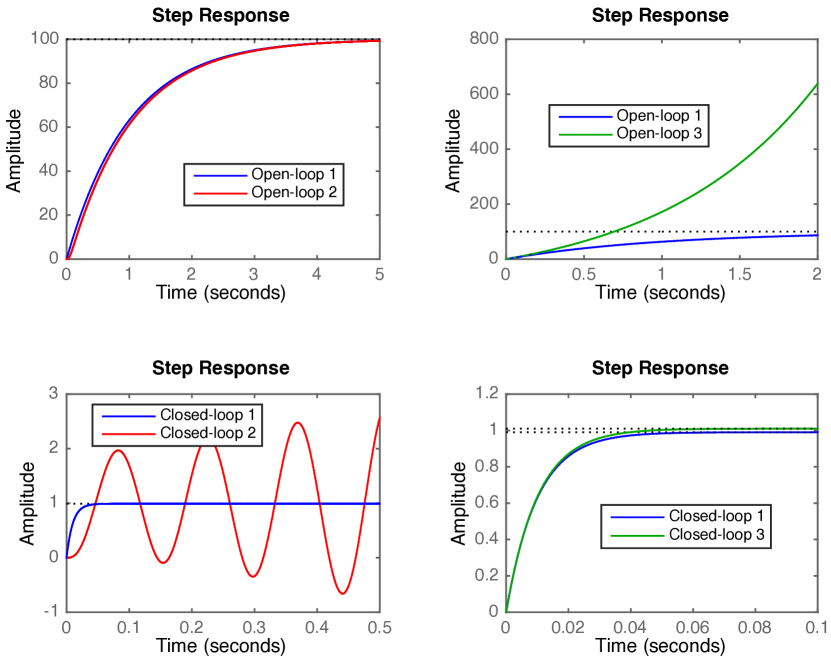
Figure 2: (Åström and Murray, 2008, Fig. 12.3) Similar open-loop responses do not imply similar closed-loop responses, and vice versa. See Åström and Murray (2008, Sect. 12.1) for details of the models, feedback policy and gap metric computations.

show that a good open-loop model is not sufficient for feedback design. The systems have similar open-loop responses, but different closed-loop responses. This is because the controller amplifies the effect of differences in open-loop dynamics, resulting in an unstable closed-loop for one system. Equally surprising, the two plots on the right of Figure 2 show that systems can have very different open-loop responses (one system is open-loop stable and the other is open-loop unstable), but virtually indistinguishable closed-loop responses. Feedback therefore allows one to tolerate large uncertainties in certain cases (the right in Figure 2), without any significant difference in closed-loop performance. However, in other cases it is critical to capture the dynamics where a poorly designed feedback algorithm could make matters worse (the left in Figure 2). A good understanding of control theory, coupled with appropriate model development, is therefore necessary to avoid designing computing systems that are over-engineered, as is the case today.

The above example partly explains why it has been difficult to use existing models from the computing systems literature when designing feedback algorithms. Queuing theory has been very successful in modeling the steady-state behavior of computing systems and networks, but has not yet been so successful in modeling the transient behavior (Hellerstein et al., 2004). Nonlinear fluid models have been widely used in modeling for network congestion control, but have not been so successful in the modeling of computing systems, because workloads have complicated characteristics, architectures are multi-tiered and the nature of the limiting resource changes with time (Hellerstein et al., 2009). Uncertainties in computing systems and networks are usually modeled as additive process noise, but this structure does not allow a stable and an unstable model to be compared. Likewise, parametric uncertainties cannot be used to model differences in the model order or time delays, especially if the delays change with time or are state-dependent.

It should be possible to extend a very sophisticated concept, developed in the control community, to the modeling of computing systems. Instead of using open-loop metrics, one could use the gap metric for determining whether two systems are similar in closed-loop (Vinnicombe, 2001; Georgiou and Smith, 1997; Lanzon and Papageorgiou, 2009; James et al., 2005). Loosely speaking, the gap from one system to another is the size of the smallest dynamical system that needs to be connected (defined in an appropriate sense) to the first system in order for the input-output responses of both systems to be the same. If two systems have a small gap between them and the same feedback algorithm is used, then it is possible to guarantee that the robustness and performance of the two closed-loop systems will be similar, as in the right half of Figure 2. If the gap between two systems are large, but the open-loop responses are similar, then it is possible that the closed-loop systems will behave very differently, as in the left half of Figure 2.

The gap metric allows one to account for dynamic and parametric uncertainty, additive disturbances as well as unstructured uncertainty, which greatly reduces the difficulty of modelling the uncertainty and hence the design of a feedback algorithm. It is also possible to account for uncertainty in the number of unstable modes or system zeros, which impose fundamental performance limitations on the design of feedback algorithms.

It will therefore be of interest to investigate whether the gap metric can be used to develop and validate first-principles and data-driven models for computing systems. This research could therefore bring about a fundamental change in the way that computing systems are modeled and feedback algorithms are designed.

2.2 Use your brain

As a first step, it will be useful to revisit first-principles methods currently used in modeling computing systems, such as queuing theory and linearized fluid flow models, but armed with the gap metric and associated control design tools. These methods could be used to analyze the robustness of existing modeling approaches and the fundamental limitations for controller design. However, it might be necessary to extend both the state of the art in modeling computing systems as well as develop techniques that are new to the control community.

Recent research on the control of infinite-dimensional systems (Jones and Kerrigan, 2010; Jones et al., 2015) has shown that, compared to using open-loop metrics, careful use of the gap metric allows one to: (i) shorten the design phase, (ii) synthesize feedback algorithms that are computationally less demanding and (iii) have stronger guarantees on the robustness and performance of the closed-loop system. One way in which the ideas in Jones and Kerrigan (2010) could potentially be applied in the control of computing systems is to approximate time delays, which are infinite-dimensional systems, with finite-dimensional input-output models and use the gap metric to provide guarantees on the closed-loop behavior. The use of Padè approximations to model time delays is a standard technique in control engineering, but does not yet seem to have found widespread use in the computing community. The gap metric can also allow one to provide robustness guarantees on the closed-loop behavior if the delay is uncertain (Cantoni et al., 2012).

An important aspect to consider in the modeling of computing systems, where research is in its early stages, is how the physics of computing systems should be incorporated into models. It is often important to consider the power consumption, heat dissipation and dynamics of the cooling system. As discussed in Section 1.2, in many cases the nodes in a distributed computing system are mobile and the physical environment could affect the performance of the network. Due to the interaction between sub-systems with discrete states, events, logic and sub-systems with continuous states and dynamics, computing systems are therefore best modeled as cyber-physical systems using techniques from hybrid dynamical systems theory (Lee and Seshia, 2014; Goebel et al., 2012).

A major open question that has to be addressed is whether nonlinear gap metric ideas (Georgiou and Smith, 1997; James et al., 2005) can be extended to certain types of hybrid systems, while allowing one to compute bounds on the gap between two systems. Furthermore, even if the model is linear, the optimal control policy is nonlinear, in general. As a consequence, there is considerable scope for extending nonlinear gap metric results for the analysis and design of model predictive controllers.

2.3 Use the data

Because of the lack of first principles models, researchers in computing systems often apply well-established, open-loop stochastic system identification methods (Ljung, 1999) to develop models from input-output data, with some success (Hellerstein et al., 2004). As a starting point for future research, it would be of interest to compare the methods currently used in the computing systems literature against recently developed methods for model validation, identification and parameter estimation of linear, nonlinear and hybrid systems (Hjalmarsson, 2005; Ljung, 2010; Paoletti et al., 2007; Betts, 2010).

However, as discussed above, it is critical to bear in mind that closed-loop measures should be used when validating or identifying models for feedback algorithm design. Gap metric ideas can also be used if input-output data is available to validate a given model (Hjalmarsson, 2005) or to compute a model directly from data using system identification methods (Date and Vinnicombe, 2004). Given some data, a model can be interpreted as sufficiently accurate if the data is consistent with what one would have measured if a small dynamical system is connected (defined in an appropriate sense) to the model. There are no published results on how closed-loop metrics can be used for model validation and identification of computing systems. Research in this area could therefore enable the development of more appropriate models and feedback algorithms, with better performance and robustness guarantees than methods based on open-loop measures.

Due to the complicated nature of the dynamics, large size and high speed of computing systems, state of the art optimization methods will be inadequate for solving many of the new model validation, identification and parameter estimation problems that will arise. Hence, novel and more efficient numerical methods will have to be developed that allow one to (in)validate, (un)falsify or identify a feedback-oriented model, ideally in real-time.

3 It Takes Time

Because time does not stop, an approximate answer today can be better than an accurate answer tomorrow. Computing systems employ feedback algorithms to cope with uncertainty, but the system is in open-loop while the computation is being carried out. Hence, it might be better to implement a simple, computationally efficient algorithm at a fast rate than a sophisticated algorithm at a slow rate.

3.1 Computing needs time

Consider a simple example, illustrated in Figure 3.

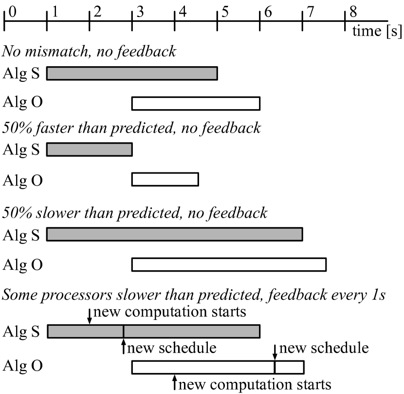
Figure 3: Comparison between two scheduling algorithms.

Suppose you have a large number of jobs that need to be completed, a large number of heterogeneous processors to do the computations and two scheduling algorithms. Algorithm O is the ‘optimal’ algorithm, which is guaranteed to find the global minimum, and Algorithm S is the ‘sub-optimal’ one, which is not guaranteed to find the global minimum or even a local minimum. Algorithm O takes 3 seconds to compute a schedule, but Algorithm S only takes 1 second. Suppose there is no mismatch between the speeds of the processors and those assumed by the algorithms. At the first scheduling event, at time $t=0$ s, both algorithms start to compute a schedule and Algorithm S terminates after 1 s with a schedule that will take 4 s from start to finish, i.e. all jobs will be completed by $t=5$ s. However, Algorithm O terminates after 3 s with a schedule that will take 3 s from start to finish, i.e. all jobs will be completed by $t=6$ s. In this case, ‘sub-optimal’ Algorithm S is better than ‘optimal’ Algorithm O, because Algorithm S gets all the jobs done before Algorithm O! Algorithm O needs to take less than 2 s to compute a solution in order to be better than Algorithm S.

The difference can be even greater if there are mismatches between the speeds of some of the processors and those assumed by the algorithms, as is also shown in Figure 3. Suppose that the processors are faster than assumed and that it takes 50% less time for jobs to complete than those predicted according to the original schedules, i.e.  the schedule computed by Algorithm S completes all jobs by $t=3$ s, which is when Algorithm O has just completed its computation (the difference between completion times is also larger). Consider the opposite case in which processors are much slower than assumed so that the original schedules take 50% longer than predicted. However, suppose now that the job completion rate of each processor is fed back every 1 s. Algorithm S can detect this information at $t=2$ s and implement a new schedule at, say, $t=2.8$ s (there are fewer uncompleted jobs, hence it takes less time to compute a schedule). It is therefore possible that Algorithm S can use the updated completion rates to find a new schedule that will get all remaining jobs completed by $t=6$ s. However, Algorithm O would detect the actual job completion rates at $t=4$ s and might only be able to implement a new schedule for the remaining jobs from, say, $t=6.3$ s, which is after the schedule computed by Algorithm S would have completed.

This example demonsrtated that a scheduling algorithm should ideally take into account the time it takes to compute a schedule and that feedback helps reduce the effect of incorrect assumptions. Most algorithms and abstractions in computing do not explicitly take the passage of time into account. Real-time operating systems are arguably not as real-time as they should be. Computing not only takes time, but needs time (Lee, 2009).

3.2 When is an optimal scheduler not optimal?

Data, tasks, processors, networking and storage need to be scheduled to meet deadlines and achieve a certain quality of service, while minimising energy usage. Scheduling problems are most naturally posed as constraint satisfaction or mathematical optimization problems. Furthermore, many well-known scheduling algorithms are feedback algorithms. Scheduling problems are perfect candidates for combining solutions from control and optimization theory.

Because the resulting optimization problems can be computationally intractable, scheduling problems have historically not been solved using numerical optimization methods. Instead, computing researchers have developed a range of computationally efficient or heuristic strategies, which are usually expressed as simple sets of rules.

In the hard real-time scheduling literature, an algorithm is often defined to be optimal if the algorithm can schedule all task-sets that can be scheduled by any other algorithm. Under very specific and often conservative assumptions on the task-sets and computer architecture, it can be shown that certain well-known classical scheduling algorithms, such as earliest deadline first or rate monotonic, are optimal in this sense. There also exists a vast array of sub-optimal scheduling algorithms and in some cases one can compute limits on the level of sub-optimality.

In many applications it makes sense to relax some hard timing constraints and replace them with soft timing constraints, where the aim is to minimize the violations. For example, in video conferencing the difference between worst-case and average bandwidth requirements can be more than one order of magnitude (Sha et al., 2004, Sect. 4.1). A user might be willing to tolerate an occasional delay or data loss, or the processor frequency could be reduced to save on power requirements. Hence, if one were to use existing hard real-time scheduling algorithms, then the computing system might be over-engineered by most measures, such as cost, energy or speed. There is therefore significant scope for improving system performance measured according to criteria other than hard time deadlines. Research could therefore be devoted to developing new methodologies to solve practical scheduling problems for which the very restrictive conditions on the task-sets and architectures, currently assumed in the classical real-time scheduling literature, can be relaxed.

There have been dramatic improvements in numerical optimization methods over the last few decades. The last few years have therefore seen a sharp increase in the use of numerical optimization methods for solving scheduling problems, mainly driven by the need to minimize energy usage in data centers and energy-limited computing devices (Li and Wu, 2013). However, much of the literature either (i) focuses on steady-state optimization, hence ignoring transients, (ii) uses open-loop dynamic models, (iii) do not explicitly account for the time taken to solve the scheduling problem, (iv) do not consider the effect of terminating the optimization solver before a solution has been found, or (v) only consider hard time constraints.

3.3 Any time in real-time predictive control

There is a clear need to develop new scheduling algorithms and abstractions that explicitly address the passage of time. This can be done by incorporating into the algorithm a time-based dynamical model of the system and uncertainties, regularly updating the algorithm with the current state of the resources and completion rates, and implementing the best available solution when further computations are not guaranteed to improve the closed-loop system performance or robustness.

It is therefore possible to take a different approach to most scheduling methods and build on recent research in efficient real-time algorithms (Bemporad et al., 2015; Domahidi et al., 2012; Diehl et al., 2002; Zavala and Anitescu, 2010; Zavala and Biegler, 2009) and computer architectures (Jerez et al., 2012, 2014) for optimization-based control. A dynamical model of the system can be used to formulate an optimization problem, which is updated at each sample instant with the latest measurements and solved using numerical optimization methods before implementing the first part of the solution. This process is then repeated at all sample instances. However, the key idea in real-time model predictive control algorithms is that one does not iterate till the algorithm has converged, but that the algorithm is allowed to terminate at any time with a potentially sub-optimal solution.

At each scheduling event, the optimization solver can be initialized with a version of the policy obtained at the previous event that is time-shifted, as in receding horizon control, or truncated, as in decreasing horizon control. Using similar arguments as in the real-time predictive control literature one should be able to construct optimization-based schedulers that will converge to a locally optimal solution after a few scheduling events, provided feedback occurs at a sufficiently fast rate. In order to take advantage of any existing and future results in the real-time scheduling literature, one can also choose to initialize the optimization solver with the policy that one would get from implementing any other rule-based or heuristic scheduling algorithm.

An anytime approach requires significantly less computational resources than iterating till an optimal solution has been found. Real-time model predictive control can allow one to implement sub-optimal solutions at a fast rate with similar or better closed-loop performance, coupled with a significant reduction in computational requirements, compared to implementing optimal solutions at a slow rate.

Provided the right algorithms and computer architectures are used, optimization-based controllers can be implemented for very fast systems with sample rates in the MHz (Jerez et al., 2014) range, and has is sufficiently efficient for controlling the speed and power dissipation of microprocessors (Mattingley et al., 2011; Zanini et al., 2013). It is clearly time for real-time model predictive control of computing systems.

3.4 Computers working together

In many computing systems today each processing unit functions in a non-cooperative, decentralised manner. Though this has allowed for the massive expansion of the Internet, this approach is not always ideal or necessary. Many high performance and embedded computing systems have custom-designed architectures and operating systems that allow the processing units to share information and resources in an effective and reliable manner. On the other hand, it is also not always sensible to have a purely centralised approach either, since expansion is difficult and the system can be more vulnerable to faults and attacks. A compromise between a fully centralised and fully decentralised approach is a cooperative distributed design, where computing units share information and resources with a common goal. Most well-known scheduling algorithms are applicable to uni-processor systems only and research on multi-processor and distributed architectures is still very much in its infancy (Davis and Burns, 2011; Li and Wu, 2013; Vidyarthi et al., 2009). There is therefore a need for research on scalable, hard and soft real-time scheduling algorithms for distributed computing systems.

Over the last decade there has been an explosion of activity in the control community in the area of distributed control of networks of dynamical systems. This activity has resulted in the development of scalable, real-time optimization-based control methods tailored to cooperative distributed systems (Christofides et al., 2013; Negenborn and Maestre, 2014). These methods could, in principle, be applied to develop scalable scheduling algorithms that enable distributed, multi-processor computing systems to cooperate in meeting overall system performance and reliability specifications.

An open problem is how best one could develop tractable methods for obtaining low-order models of physically distributed computing systems. The problem with most model reduction methods (Antoulas, 2005) is that they require a high-order model. The gap-metric based approach in Jones and Kerrigan (2010) is fundamentally different and does not require a high-order model, hence is computationally more efficient, while still providing guarantees on the robustness and performance of the closed-loop system. By gradually increasing the model complexity, convergence of the model sequence happens faster with closed-loop metrics than with open-loop metrics. Another advantage is that the resulting model retains the structure and sparsity of the original. This structure can be exploited by numerical algorithms for design and implementation, whereas most model reduction methods destroy structure and sparsity. It might therefore be possible to use gap metric ideas to produce scalable, distributed models and account for the effect of communication faults and delays, changes in the structure of the communication and computation networks, as well as variability in resources.

3.5 When is tailor-made not a luxury?

As illustrated in Figure 3, the computational resources used by an algorithm has to be sufficiently small. Most off-the-shelf optimization solvers are not able to exploit the special structure that is present in scheduling problems. Therefore, tailor-made methods have to be developed that are better than the state of the art by exploiting any structure that is present in the scheduling problem.

The structure can be exploited by formulating the scheduling problem as a multistage optimization problem, as is done in optimization-based control (Betts, 2010), and solving this efficiently with the aid of sparse linear algebra. Efficient mixed-integer optimization algorithms for optimal control of systems with integer decision variables (Sager, 2006) could be explored in this context. It might also be possible to derive conditions under which the scheduling problem can be formulated as a convex and tractable optimization problem, e.g. in De Schutter and van den Boom (2001) conditions are derived under which the optimal control of max-plus-linear discrete event systems can be formulated as a computationally tractable linear program.

In many scheduling problems, it is natural to introduce integer variables and solve a mixed-integer program. In some cases it might be better to model the problem as a continuous optimization problem without integer variables. For example, suppose there is a large number of jobs that can be grouped into a relatively small number of subsets. and that there is a relatively small number of identical processors. The decision variables in the optimization solver can include the fraction of jobs from each subset that are allocated to a percentage of a processor’s time, as in deadline partitioning techniques (Levin et al., 2010). This results in smaller and ‘nicer’ optimization problems than using binary variables to assign jobs to processors.

Another question is how best to incorporate deterministic and stochastic uncertainties into the formulation of the optimization problem. Robust optimization methods (Ben-Tal et al., 2009) might then be used to efficiently solve scheduling problems subject to uncertainties. One of the main ideas that can be explored is how to formulate the scheduling problem as an optimal control problem where the optimization is over feedback policies (Goulart et al., 2006), rather than open-loop input sequences.

In some cases it might be best to use parametric programming (Borrelli, 2003) techniques to compute an explicit solution to the optimization problem. The scheduling algorithm can then be implemented as a lookup table, similar to the way classical scheduling algorithms are implemented as a set of rules, but with guarantees of optimality and with more flexibility in the nature of the assumptions on the task-sets and architectures. The disadvantage is that often the size of the look-up table blows up for large problem sizes. Parametric programming might therefore be best suited to small-scale computing systems, such as multi-core processors (Zanini et al., 2013).

Many optimization methods cannot be terminated at any time with a guarantee that sub-optimal iterates will reduce the cost, satisfy all constraints or guarantee closed-loop stability or robustness. Possible solutions that one could investigate including adding constraints or modifying the cost function to enforce cost reduction, constraint satisfaction and closed-loop stability (Bemporad et al., 2015; Domahidi et al., 2012; Scokaert et al., 1999). The modified algorithm might take longer to converge, but can be terminated at any time with an improved strategy, with better closed-loop performance and robustness.

Finally, one should consider what effect the architecture of the computing system has on the computational requirements. Field Programmable Gate Arrays (FPGAs) and Graphical Processing Units (GPUs) can also be used to explore the use of parallelism and custom number representations to reduce the computational requirements. Can the architecture be designed to allow for the development of better scheduling algorithms?

4 Opportunities and More Problems

There is tremendous opportunity for control and optimization to make a big impact in the area of computing systems. By combining gap metric ideas with real-time model predictive control methods to design new scheduling algorithms, one might be able to design computing systems that are at least one order of magnitude faster, cheaper, more energy efficient and more reliable, compared to using state of the art open-loop models and classical real-time scheduling algorithms.

Because of the range in complexity, size and speed of computing systems, there is also a vast array of problems that will challenge control and optimization theory. By solving some of these problems, new methods will result that can also be applied outside the computing domain, e.g. in power, manufacturing, transport and healthcare, where similar control and optimization problems arise.

References

- Antoulas (2005) Antoulas, A.C. (2005). Approximation of Large-Scale Dynamical Systems. SIAM.
- Åström and Murray (2008) Åström, K.J. and Murray, R.M. (2008). Feedback Systems: An Introduction for Scientists and Engineers. Princeton University Press.
- Bemporad et al. (2015) Bemporad, A., Bernardini, D., and Patrinos, P. (2015). A convex feasibility approach to anytime model predictive control. CoRR, abs/1502.07974. URL http://arxiv.org/abs/1502.07974.
- Ben-Tal et al. (2009) Ben-Tal, A., El Ghaoui, L., and Nemirovski, A. (2009). Robust Optimization. Princeton University Press.
- Betts (2010) Betts, J.T. (2010). Practical Methods for Optimal Control and Estimation Using Nonlinear Programming. SIAM, 2nd edition.
- Borrelli (2003) Borrelli, F. (2003). Constrained Optimal Control of Linear and Hybrid Systems. Springer-Verlag.
- Cantoni et al. (2012) Cantoni, M., Jonsson, U.T., and Kao, C. (2012). Robustness analysis for feedback interconnections of distributed systems via integral quadratic constraints. Automatic Control, IEEE Transactions on, 57(2), 302–317. 10.1109/TAC.2011.2163335.
- Christofides et al. (2013) Christofides, P.D., Scattolini, R., de la Peña, D.M., and Liu, J. (2013). Distributed model predictive control: A tutorial review and future research directions. Computers and Chemical Engineering, 51(0), 21–41.
- Date and Vinnicombe (2004) Date, P. and Vinnicombe, G. (2004). Algorithms for worst case identification in and in the -gap metric. Automatica, 40(6), 995–1002.
- Davis and Burns (2011) Davis, R.I. and Burns, A. (2011). A survey of hard real-time scheduling for multiprocessor systems. ACM Comput. Surv., 43(4), 35:1–35:44.
- De Schutter and van den Boom (2001) De Schutter, B. and van den Boom, T.J.J. (2001). Model predictive control for max-plus-linear discrete event systems. Automatica, 37(7), 1049–1056.
- Diehl et al. (2002) Diehl, M., Bock, H.G., Schlöder, J.P., Findeisen, R., Nagy, Z., and Allgöwer, F. (2002). Real-time optimization and nonlinear model predictive control of processes governed by differential-algebraic equations. J. Process Control, 12(4), 577–585.
- Domahidi et al. (2012) Domahidi, A., Zgraggen, A.U., Zeilinger, M.N., Morari, M., and Jones, C.N. (2012). Efficient interior point methods for multistage problems arising in receding horizon control. In Proc. 51 IEEE Conf. Decision and Control, 668–674.
- Georgiou and Smith (1997) Georgiou, T.T. and Smith, M.C. (1997). Robustness analysis of nonlinear feedback systems: An input-output approach. IEEE Trans. Automatic Control, 42(9), 1200–1221.
- GeSI (2012) GeSI (2012). SMARTer 2020: The role of ICT in driving a sustainable future. http://gesi.org/SMARTer2020.
- Goebel et al. (2012) Goebel, R., Sanfelice, R.G., and Teel, A.R. (2012). Hybrid Dynamical Systems: Modeling, Stability, and Robustness. Princeton University Press.
- Goulart et al. (2006) Goulart, P.J., Kerrigan, E.C., and Maciejowski, J.M. (2006). Optimization over state feedback policies for robust control with constraints. Automatica, 42(4), 523–533.
- Hellerstein et al. (2004) Hellerstein, J.L., Dao, Y., Parekh, S., and Tilbury, D.M. (2004). Feedback Control of Computing Systems. John Wiley & Sons Inc.
- Hellerstein et al. (2009) Hellerstein, J.L., Singhal, S., and Wang, Q. (2009). Research challenges in control engineering of computing systems. IEEE Trans. Network and Service Management, 6(4), 206–211.
- Hjalmarsson (2005) Hjalmarsson, H. (2005). From experiment design to closed-loop control. Automatica, 41(3), 393–438.
- James et al. (2005) James, M., Smith, M.C., and Vinnicombe, G. (2005). Gap metrics, representations, and nonlinear robust stability. SIAM Journal on Control and Optimization, 43(5), 1535–1582.
- Jerez et al. (2012) Jerez, J.L., Ling, K.V., Constantinides, G.A., and Kerrigan, E.C. (2012). Model predictive control for deeply pipelined field-programmable gate array implementation: algorithms and circuitry. IET Control Theory & Applications, 6(8), 1029–1041.
- Jerez et al. (2014) Jerez, J.L., Richter, S., Goulart, P.J., Constantinides, G.A., Kerrigan, E.C., and Morari, M. (2014). Embedded online optimization for model predictive control at megahertz rates. Automatic Control, IEEE Transactions on, 59(12), 3238–3251. 10.1109/TAC.2014.2351991.
- Jones et al. (2015) Jones, B.L., Heins, P.H., Kerrigan, E.C., Morrison, J.F., and Sharma, A.S. (2015). Modelling for robust feedback control of fluid flows. J. Fluid Mechanics, 769, 687–722.
- Jones and Kerrigan (2010) Jones, B.L. and Kerrigan, E.C. (2010). When is the discretization of a spatially distributed system good enough for control? Automatica, 46(9), 1462–1468.
- Lanzon and Papageorgiou (2009) Lanzon, A. and Papageorgiou, G. (2009). Distance measures for uncertain linear systems: A general theory. IEEE Trans. Automatic Control, 54(7), 1532–1547.
- Lee (2009) Lee, E.A. (2009). Computing needs time. Commun. ACM, 52(5), 70–79.
- Lee and Seshia (2014) Lee, E.A. and Seshia, S.A. (2014). Introduction to Embedded Systems: A Cyber-Physical Systems Approach. http://LeeSeshia.org, 1.5 edition.
- Levin et al. (2010) Levin, G., Funk, S., Sadowski, C., Pye, I., and Brandt, S. (2010). DP-FAIR: A simple model for understanding optimal multiprocessor scheduling. In Real-Time Systems (ECRTS), 2010 22nd Euromicro Conference on, 3–13. 10.1109/ECRTS.2010.34.
- Li and Wu (2013) Li, D. and Wu, J. (2013). Energy-aware Scheduling on Multiprocessor Platforms. Springer.
- Ljung (1999) Ljung, L. (1999). System Identification: Theory for the User. Prentice Hall, 2nd edition.
- Ljung (2010) Ljung, L. (2010). Perspectives on system identification. Annual Reviews in Control, 34(1), 1–12.
- Mattingley et al. (2011) Mattingley, J., Wang, Y., and Boyd, S. (2011). Receding horizon control. IEEE Control Systems, 31(3), 52–65.
- Mayne (2014) Mayne, D.Q. (2014). Model predictive control: Recent developments and future promise. Automatica, 50(12), 2967–2986.
- Negenborn and Maestre (2014) Negenborn, R.R. and Maestre, J.M. (2014). Distributed model predictive control: An overview and roadmap of future research opportunities. IEEE Control Systems, 34(4), 87–97.
- Paoletti et al. (2007) Paoletti, S., Juloski, A.L., Ferrari-Trecate, G., and Vidal, R. (2007). Indentification of hybrid systems: A tutorial. European J. Control, 13(2–3), 242–260.
- Sager (2006) Sager, S. (2006). Numerical methods for mixed-integer optimal control problems. Ph.D. thesis, University of Heidelberg.
- Scokaert et al. (1999) Scokaert, P.O.M., Mayne, D.Q., and Rawlings, J.B. (1999). Suboptimal model predictive control (feasibility implies stability). IEEE Trans. Automatic Control, 44(3), 648–654.
- Sha et al. (2004) Sha, L., Abdelzaher, T., Årzén, K.E., Cervin, A., Baker, T., Burns, A., Buttazzo, G., Caccamo, M., Lehoczky, K., and Mok, A.K. (2004). Real time scheduling theory: A historical perspective. Real-Time Systems, 28, 101–155.
- Vereecken et al. (2010) Vereecken, W., Van Heddeghem, W., Colle, D., Pickavet, M., and Demeester, P. (2010). Overall ICT footprint and green communication technologies. In Proc. 4th International Symposium on Communications, Control and Signal Processing (ISCCSP 2010).
- Vidyarthi et al. (2009) Vidyarthi, D.P., Sarker, B.K., Tripathi, A.K., and Yang, L.T. (2009). Scheduling in Distributed Computing Systems: Analysis, Design and Models. Springer.
- Vinnicombe (2001) Vinnicombe, G. (2001). Uncertainty and Feedback: loop-shaping and the -gap metric. Imperial College Press.
- Zanini et al. (2013) Zanini, F., Atienza, D., Jones, C.N., Benini, L., and De Micheli, G. (2013). Online thermal control methods for multiprocessor systems. ACM Trans. Des. Autom. Electron. Syst., 18(1), 6:1–6:26. 10.1145/2390191.2390197. URL http://doi.acm.org/10.1145/2390191.2390197.
- Zavala and Anitescu (2010) Zavala, V. and Anitescu, M. (2010). Real-time nonlinear optimization as a generalized equation. SIAM Journal on Control and Optimization, 48(8), 5444–5467.
- Zavala and Biegler (2009) Zavala, V.M. and Biegler, L.T. (2009). The advanced-step NMPC controller: Optimality, stability and robustness. Automatica, 45(1), 86–93.