Bregman Iteration for Correspondence Problems

Abstract

Bregman iterations are known to yield excellent results for denoising, deblurring and compressed sensing tasks, but so far this technique has rarely been used for other image processing problems. In this paper we give a thorough description of the Bregman iteration, unifying thereby results of different authors within a common framework. Then we show how to adapt the split Bregman iteration, originally developed by Goldstein and Osher for image restoration purposes, to optical flow which is a fundamental correspondence problem in computer vision. We consider some classic and modern optical flow models and present detailed algorithms that exhibit the benefits of the Bregman iteration. By making use of the results of the Bregman framework, we address the issues of convergence and error estimation for the algorithms. Numerical examples complement the theoretical part.

1 Introduction

In 2005, Osher et al. Osher2005 proposed an algorithm for the iterative regularisation of inverse problems that was based on findings of Bregman Bregman1967 . They used this algorithm, nowadays called Bregman iteration, for image restoration purposes such as denoising and deblurring. Especially in combination with the Rudin-Osher-Fatemi (ROF) model for denoising ROF92 they were able to produce excellent results. Their findings caused a subsequent surge of interest in the Bregman iteration. Among the numerous application fields, it has for example been used to solve the basis pursuit problem Cai2009 ; Osher2008 ; Yin2007 and was later applied to medical imaging problems in Lin2006 . Further applications include deconvolution and sparse reconstructions ZBBO09 , wavelet based denoising Xu2006 , and nonlinear inverse scale space methods Burger2006 ; Burger2005 . An important adaptation of the Bregman iteration is the split Bregman method (SBM) Goldstein2009 and the linearised Bregman approach Cai2009 . The SBM can be used to solve $L_{1}$-regularised inverse problems in an efficient way. Its benefits stem from the fact that differentiability is not a necessary requirement on the underlying model and that it decomposes the original optimisation task in a series of significantly easier problems that can be solved very efficiently, especially on parallel architectures. The Bregman algorithms belong to the family of splitting schemes as well as to the primal-dual algorithms E2009 ; Setzer2009 which enjoy great popularity in the domain of image processing and which are still a very active field of ongoing research ODBP2015 ; GLY2015 .

The aim of this paper is to contribute to the mathematical foundation of the rapidly evolving area of computer vision. We explore the use of the Bregman framework, especially the application of the split Bregman method, for the problem of optical flow (OF) which is of fundamental importance in that field, cf. Aubert2006 ; KSK98 ; TV98 . We give a thorough discussion of the Bregman framework, thereby unifying results of several recent works. Then we show how to adapt the SBM to several classic and modern OF models. Detailed descriptions of corresponding algorithms are presented. Employing the Bregman framework, we show that convergence for these methods can be established and error estimates can be given.

1.1 The optical flow problem

The OF problem is an ill-posed inverse problem. It consists in determining the displacement field between different frames of a given image sequence by looking for correspondences between pixels. In many cases such correspondences are not unique or simply fail to exist because of various problems such as noise, illumination changes and overlapping objects. Nevertheless, the study of the OF problem is of fundamental importance for dealing with correspondence problems such as stereo vision where accurate flow fields are necessary BS07 ; MMK98 ; SBW2005 ; MJBB2015 . For solving the OF problem in a robust way, variational formulations and regularisation strategies belong to the most successful techniques. Those methods have been studied for almost three decades, starting from the approach of Horn and Schunck HS81 . During this period of time, many efforts have been spent to improve the models cf. BA96 ; ZBWS09 ; BBPW04 ; MP02 ; NBK08 ; WCPB09 ; WPB10 ; XJM10 ; ZBWVSRS09 ; BZW2011 ; ZBW2011 for an account of that field.

While many developments have been made on the modelling side, there are just a few works concerned with the mathematical validation of algorithms. In ki08 ; mm04 it has been shown that the classic numerical approach of Horn and Schunck converges. Furthermore, the authors of mm04 showed that the linear system obtained through the Euler-Lagrange equations has a symmetric and positive definite matrix and thus allows the usage of many efficient solvers. The authors of Wedel2008 ; Pock2007 developed an algorithm that solves the so called TV-$L^{1}$ model through an alternating minimisation scheme. This is applied to a variational formulation that augments the original energy functional with an additional quadratic term. This quadratic term allows the authors to divide their objective into simpler subproblems for which efficient solvers exist. In practice their approach yields excellent results. However, in general it does not converge towards the solution of the original energy functional but to a solution of the augmented variational formulation. Alternative approaches to minimise the occurring variational models include CP2011 ; OCBP2014 ; OBP2015 . These well performing algorithms possess good convergence properties, but may require additional regularity conditions, such as strong convexity of the considered energy, see OBP2015 . The author of br06 discusses the usage of efficient algorithms such as the Multigrid approach B1973 ; BL2011 ; BHM00 ; Hac85 ; Wes92 and the so called Lagged-Diffusivity or Kac̆anov method CM99 ; FKN73 ; KNPS68 . Finally, it is also possible to consider the solutions of the Euler-Lagrange equations as a steady-state of a corresponding diffusion-reaction system that one may solve by means of a steepest descend approach wb05 ; WBPB04 . Recent developments have extended the study of the OF problem onto dynamic non-Euclidean settings where the motion is estimated on an evolving surface KLS2015 . Other trends include the use of powerful (deep) learning strategies SRLB2008 ; DFIH2015 or even combinations of variational and machine learning approaches WRHS2013 .

1.2 Our contribution

We present an approach to the OF problem by exploring the Bregman framework. Despite their usefulness, Bregman iterations have received little attention in the context of OF up to now. Early attempts inlcude LBS2010 ; H2010 . Here, we propose mathematically validated methods for OF models, among them the prominent model of Brox et al. BBPW04 .

The main contribution of this work lies in the thorough presentation of the Bregman framework and the proof of convergence of the algorithms in the context of OF, thus giving the numerical solution of the OF problem a solid mathematical basis. To this end, we adapt the general convergence theory of the Bregman framework to the OF algorithms and show that the SBM iterates converge towards a minimiser of the considered energy functionals. Related questions that are important in the context of the numerical processing will also be discussed here. For instance, we will show that the arising linear systems have a symmetric and positive definite matrix. The assumptions for this are quite weak and naturally met in almost all setups.

1.3 Paper Organisation

In Section 2, we give a brief account of mathematical prerequisites, whereas Section 3 elaborates on the Bregman framework. Next, in Section 4 we give an account of the OF models we consider, and how to formulate the corresponding algorithms in terms of the SBM. Finally, we complement the theoretical developments by some numerical experiments given in Section 5 and finish the paper by some conclusions.

2 Mathematical prerequisites

In this work we strongly rely on the notion of subdifferentiability as it grants us the ability to handle non-differentiable robust regularisers, such as the $\ell_{1}$ norm, in similar style as smooth functions. For a thorough analysis of this important concept in convex optimisation we refer to the excellent presentations in Ekeland1999 ; Rockafellar1997 ; rj98 . Here, we merely recall the definition of a subdifferential. The subdifferential $\partial\varphi\left(\bar{x}\right)$ of a function $\varphi\colon{}\mathbb{R}^{n}\to\mathbb{R}\cup\left\{+\infty\right\}$ at position $\bar{x}$ is a set valued mapping given by

$$\partial\varphi\left(\bar{x}\right)\coloneqq\left\{x^{*}\middle|\ \varphi\left(x\right)-\varphi\left(\bar{x}\right)\geqslant\langle x^{*},x-\bar{x}\rangle,\ \forall x\right\}\enspace{}.$$ (1)

Its elements are called subgradients. Without further requirements on $\varphi$ this set may contain infinitely many elements or be empty. A common example is the subgradient of the absolute value function where a simple computation shows that

$$\partial\left(\left|\>\cdot\>\right|\right)\left(x\right)=\begin{cases}\left\{-1\right\},&x<0\enspace{},\\ \left[-1,1\right],&x=0\enspace{},\\ \left\{1\right\},&x>0\enspace{}.\end{cases}$$ (2)

For strictly concave functions the subdifferential is always empty. On the other hand, convex functions always have a least one subgradient in the interior of their domain. Subdifferentials exhibit many properties of usual derivatives. One of the most important properties of subdifferentials is for example that $0\in\partial\varphi\left(\bar{x}\right)$ is a necessary condition for $\bar{x}$ being a minimiser of $\varphi$.

Robust regularisers involving the $\ell_{1}$ norm are quite common in variational image analysis models. Their optimisation often leads to subproblems of the kind

$$\operatorname*{arg\,min}_{x\in\mathbb{R}^{n}}\left\{\left\|x\right\|_{1}+\frac{\lambda}{2}\left\|x-b\right\|_{2}^{2}\right\}$$ (3)

with a positive parameter $\lambda$ and an arbitrary vector $b$. A closed form solution $x^{*}$ can be derived in terms of the well known soft shrinkage operator: $x^{*}=\operatorname{shrink}(b,\frac{1}{\lambda})$, where

$$\operatorname{shrink}\left(y,\alpha\right)\coloneqq\begin{cases}y-\alpha,&y>\alpha\enspace{},\\ 0,&y\in\left[-\alpha,\alpha\right]\enspace{},\\ y+\alpha,&y<-\alpha\enspace{}.\end{cases}$$ (4)

For vector valued arguments, the shrinkage operator is applied componentwise. Unfortunately, the $\ell_{1}$ norm is not rotationally invariant and promotes in many applications undesired structures parallel to the coordinate axes. A possible workaround consists in adapting the considered models such that we are lead to tasks of the form

$$\operatorname*{arg\,min}_{x\in\mathbb{R}^{n}}\left\{\left\|x\right\|_{2}+\frac{\lambda}{2}\left\|x-b\right\|_{2}^{2}\right\}$$ (5)

with $\lambda>0$. Here, the closed form solution can be expressed in terms of the generalised shrinkage operator.

Definition 1 (Generalised Shrinkage)

Let $b$ be a vector in $\mathbb{R}^{n}$ and $\lambda>0$, then we define the generalised shrinkage operator as

$$\begin{split}\operatorname{gshrink}\left(b,\lambda\right)&\coloneqq\max\left(\left\|b\right\|_{2}-\lambda,0\right)\frac{b}{\left\|b\right\|_{2}}\phantom{:}=\begin{cases}b-\frac{\lambda}{\left\|b\right\|}_{2}b,&\text{if}\ \left\|b\right\|_{2}>\lambda\enspace{},\\ 0,&\text{else}\enspace{},\end{cases}\end{split}$$ (6)

where we adopt the convention $0\cdot\frac{0}{0}=0$.

The solutions $x^{*}$ of (5) can then be expressed in term of this generalised shrinkage. It holds $x^{*}=\operatorname{gshrink}\left(b,\frac{1}{\lambda}\right)$. The proof is lengthy but not difficult. One has to find those $x^{*}$ for which 0 is a subgradient of the cost function. This can be done by discerning the cases $\lambda\left\|b\right\|_{2}>1$ and $\lambda\left\|b\right\|_{2}\leqslant 1$.

3 The Bregman Framework

We begin with recalling the standard Bregman iteration as developed by Osher et al. Osher2005 . Furthermore, we present an alternative but equivalent formulation of the Bregman algorithm which has been discussed in Goldstein2009 . We make use of this formulation as it simplifies the proof of a convergence assertion and for describing the SBM introduced by Goldstein and Osher Goldstein2009 . As indicated, the SBM will be the basis for our OF algorithms. Let us emphasise that many approaches to the Bregman framework exist in the literature. Bregman himself Bregman1967 wanted to describe non-orthogonal projections onto convex sets. Further research in that direction can for example be found in BB1997 . In E2009 ; Setzer2009 a certain number of equivalences between different optimisation techniques are discussed. They allow us to interpret the Bregman algorithms by means of conjugate duality for convex optimisation. Thus, the Bregman framework may also be interpreted as a splitting scheme or a primal dual algorithm. The presentation in this work relies more on similarities between constrained and unconstrained convex optimisation problems. The convergence theory that we will recall and present here is based on results in Brune2009 ; Burger2006 ; BRH07 ; Cai2009a ; Goldstein2009 ; Osher2005 . The authors of these works employed different mathematical settings. Some of the results require Hilbert spaces, others are stated in rather general vector spaces only equipped with semi-norms. We unify the results here within one framework using finite dimensional, normed vector spaces. This set-up allows the usage of a common set of requirements and to clarify relations between the different works. While doing this, we also add some new results to the SBM.

We note that this mathematical setting suffices for the typical application in computer vision where one ultimately needs to resort to a discretised problem.

Let us now introduce the mathematical formalism that we will require in the forthcoming sections. One of the central concepts behind the Bregman iteration is the Bregman divergence. It has been presented by Bregman in 1967 Bregman1967 , where it has been used to solve convex optimisation problems through non-orthogonal projections onto convex sets.

Definition 2 (Bregman Divergence)

The Bregman divergence $D_{\varphi}^{p}\colon\mathbb{R}^{n}\times\mathbb{R}^{n}\to\mathbb{R}$ of a proper convex function $\varphi$ is defined as $D_{\varphi}^{p}\left(x,y\right)\coloneqq\varphi\left(x\right)-\varphi\left(y\right)-\langle p,x-y\rangle$. Thereby $p$ is a subgradient of $\varphi$ at $y$.

The aim of the Bregman iteration is to have a formulation that can handle convex non-differentiable cost functions and that avoids ill conditioned formulations. To illustrate the main idea, one may consider e.g. the following optimisation problem:

$$x^{(k+1)}=\operatorname*{arg\,min}_{x\in\mathbb{R}^{n}}\ \left\{D_{\varphi}^{p}\left(x,x^{(k)}\right)+\iota_{\left\{0\right\}}\left(Ax-b\right)\right\}$$ (7)

where $\iota_{S}$ is the indicator function of the set $S$, i.e. $\iota_{S}(x)$ is 0 if $x\in S$ and $+\infty$ else. In case the linear system $Ax=b$ has multiple solutions or if it has a very large system matrix, then it might be difficult to determine the iterates $x^{(k)}$. Therefore, one may reformulate (7) in terms of a regularised and unconstrained problem

$$x^{(k+1)}=\operatorname*{arg\,min}_{x\in\mathbb{R}^{n}}\left\{D_{\varphi}^{p}\left(x,x^{(k)}\right)+\lambda\left\|Ax-b\right\|_{2}^{2}\right\}$$ (8)

with some fixed $\lambda>0$ to approximate (7). This iterative strategy motivates Definition 3, which coincides with the formulation found in Goldstein2009 ; Osher2005 ; Yin2007 .

Let us note that in Osher2005 ; Yin2007 the Bregman iteration has been formulated as a method for minimising convex functionals of the form $J\left(u\right)+H\left(u\right)$. However, the convergence theory presented below that is derived from Brune2009 ; Burger2006 ; BRH07 ; Cai2009a ; Goldstein2009 ; Osher2005 states that the iterates converge towards the solution of a constrained formulation. Therefore, we define the algorithm from the beginning on as a method for solving constrained optimisation problems. In the following we silently assume that $J$ and $H$ are always two proper convex functions defined on the whole $\mathbb{R}^{n}$. Further, $H$ will be a non-negative differentiable function with $0=\min_{u}\left\{H\left(u\right)\right\}$ and this minimum is reached at some point in $\mathbb{R}^{n}$.

Definition 3 (Bregman iteration)

The Bregman iteration of the constrained optimisation problem

$$\operatorname*{arg\,min}_{u\in\mathbb{R}^{{n}}}\left\{J\left(u\right)+\iota_{\left\{0\right\}}\left(H\left(u\right)\right)\right\}$$ (9)

is given by:

1. Choose $u^{(0)}$ arbitrarily, $\lambda>0$ and $p^{(0)}\in\partial J\left(u^{(0)}\right)$.

2. Compute iteratively

   $$u^{(k+1)}=\operatorname*{arg\,min}_{u\in\mathbb{R}^{{n}}}\left\{D_{J}^{p^{(k)}}\left(u,u^{(k)}\right)+\lambda H\left(u\right)\right\}\\$$ (10)

   where we have $p^{(k)}\in\partial J\left(u^{(k)}\right)$ until a fixed-point is reached.

From our assumptions on $J$ it follows that it has at least one subgradient at every point. Thus $p^{(k)}$ always exists, but it is not necessarily unique. In general settings the computation of a subgradient may not always be simple. The following result from Yin2007 provides a comfortable strategy to obtain a single specific subgradient.

Proposition 1

If $H$ is differentiable, the second step of the Bregman iteration from Definition 3 becomes

$$\begin{split}u^{(k+1)}&=\operatorname*{arg\,min}_{u\in\mathbb{R}^{n}}\left\{D_{J}^{p^{(k)}}\left(u,u^{(k)}\right)+\lambda H\left(u\right)\right\}\enspace{},\\ p^{(k+1)}&=p^{(k)}-\lambda\nabla H\left(u^{(k+1)}\right)\enspace{}.\end{split}$$ (11)

Proof

It suffices to show that $p^{(k)}-\lambda\nabla H(u^{(k+1)})$ is a subgradient of $J$ at position $u^{(k+1)}$. The definition of the iterates $(u^{(k)})_{k}$ implies that $u^{(k+1)}$ is a minimiser of $D_{J}^{p^{(k)}}(u,u^{(k)})+\lambda H\left(u\right)$. Expanding the definition of the Bregman divergence and removing the constant terms, we see that $0$ is a subgradient of $J(u)-\langle p^{(k)},u\rangle+\lambda H(u)$ at position $u^{(k+1)}$. Since the subdifferential of a sum coincides with the sum of the subdifferentials it follows that there must exist $p^{(k+1)}\in\partial J(u^{(k+1)})$ that fulfils the equation

$$0=p^{(k+1)}-p^{(k)}+\lambda\nabla H\left(u^{(k+1)}\right)\enspace{}.$$ (12)

Although one could basically use any subgradient of $J$ at $u^{(k+1)}$, the previous proposition gives us a convenient way of finding a specific one that is easy to obtain. This makes the computation of the iterates much simpler and improves the overall speed of the algorithm.

Our next goal is to analyse the convergence behaviour of the Bregman iteration given in Definition 3, and to show that its iterates obtained from

$$\operatorname*{arg\,min}_{u\in\mathbb{R}^{n}}\ \left\{D_{J}^{p^{(k)}}\left(u,u^{(k)}\right)+\lambda H\left(u\right)\right\}$$ (13)

converge towards a solution of

$$\operatorname*{arg\,min}_{u\in\mathbb{R}^{n}}\left\{J\left(u\right)+\iota_{\left\{0\right\}}\left(H\left(u\right)\right)\right\}\enspace{}.$$ (14)

For well-posedness reasons we will assume that (14) as well as the iterative formulation in (13) are always solvable. If these requirements are not feasible, then our iterative strategy cannot be carried out or fails to converge. We emphasise that the existence of a solution of either (13) or (14) cannot always be deduced from the existence of the other formulation. Even if $H(u)=0$ cannot be fulfilled, it might still be possible that all iterates in (13) exist.

The results compiled by the Propositions 2, 3, and 4, as well as Corollary 1 were already discussed in Osher2005 . There, the authors discussed iterative regularisation strategies in the space of functions with bounded variation. Furthermore, they established the link between their algorithm and the Bregman divergence. The proofs from Osher2005 for the variational setting carry over verbatim to the finite dimensional set-up that we use within this work. Thus, we just recall the statements without proofs.

Proposition 2

The sequence $(H(u^{(k)}))_{k}$ is monotonically decreasing. We have for all $k$:

$$H\left(u^{(k+1)}\right)\leqslant H\left(u^{(k)}\right)$$ (15)

and strict inequality when $D_{J}^{p^{(k)}}(u^{(k+1)},u^{(k)})$ is positive.

In this context we remark that the Bregman divergence is always non-negative for convex $J$ and if $J$ is even strictly convex, then $D_{J}^{p}(x,y)=0$ can only hold if and only if $x=y$.

Proposition 3

We have for all $\lambda>0$

$$D^{p^{(k)}}_{J}\left(u,u^{(k)}\right)+D^{p^{(k-1)}}_{J}\left(u^{(k)},u^{(k-1)}\right)\\ -D^{p^{(k-1)}}_{J}\left(u,u^{(k-1)}\right)\leqslant\lambda\left(H\left(u\right)-H\left(u^{(k)}\right)\right).$$ (16)

Corollary 1

For the particular choice $u=\tilde{u}$, where $\tilde{u}$ is a solution of $H\left(u\right)=0$ we immediately get:

$$0\leqslant D^{p^{(k)}}_{J}\left(\tilde{u},u^{(k)}\right)\leqslant D^{p^{(k-1)}}_{J}\left(\tilde{u},u^{(k-1)}\right)\enspace{}.$$ (17)

One can easily infer from the above assertions, that for strictly convex $J$, the iterates converge towards a solution of $H(u)=0$. The next proposition gives an estimate how fast this convergence is, and it shows that the strict convexity is in fact not necessary. Let us note that the proof of it relies on the Propositions 2 and 3.

Proposition 4

If $\tilde{u}$ is a solution of $H(u)=0$ and if $D_{J}^{p^{(0)}}\left(\tilde{u},u^{(0)}\right)<+\infty$ for some starting value $u^{(0)}$ then one obtains for all $\lambda>0$

$$0=H\left(\tilde{u}\right)\leqslant H\left(u^{(k)}\right)\leqslant\frac{D_{J}^{p^{(0)}}\left(\tilde{u},u^{(0)}\right)}{\lambda k}\enspace{}.$$ (18)

Therefore, the iterates $u^{(k)}$ always converge towards a solution of $H$.

So far we have seen that the iterates converge towards a solution of $H$. But at this point we do not know whether this solution also minimises our cost function $J$. If $H$ has a unique solution, then the above theory is already sufficient.

The following proposition states, that under certain assumptions, the iterates that solve $H$ also minimise our cost function, even if $H$ has multiple solutions. This highly important result was first pointed out in Yin2007 , where the authors analysed the convergence behaviour of the Bregman iteration within the context of the basis pursuit problem. There, the authors analysed the Bregman framework in a finite dimensional setting and further showed an interesting relationship to augmented Lagrangian methods.

Proposition 5

Assume there exists $u^{(0)}$ such that it is possible to choose $p^{(0)}=0$ in (11). Furthermore, assume that $H\left(u\right)=h\left(Au-b\right)$ where $A$ is some matrix, $b$ an arbitrary vector and $h$ is a differentiable non-negative convex function that only vanishes at $0$. If an iterate $u^{(k)}$ fulfils $H(u^{(k)})=0$, i.e. it solves $Au=b$, then that iterate is also a solution of the constrained optimisation problem of (9).

Concerning the proof of Proposition 5 from Yin2007 , let us note that this proposition requires that $h$ vanishes only at $0$. However, the linear system $Au=b$ can have multiple solutions. Thus $H$ can have multiple solutions, too. The requirement that $h$ only vanishes at $0$ is essential in the proof, as it enforces that every zero of $H$ solves the linear system.

We conclude that convergence is guaranteed if $H$ has the form described in Proposition 5 and if we can choose $u^{(0)}$ such that $p^{(0)}=0$ is a valid subgradient. The latter requirement is in fact rather weak such that only the former is of importance. For the formulation of the OF problems, these conditions will fit naturally into the modelling.

We will now focus on the special case of interest for us that $h\left(x\right)\coloneqq\left\|x\right\|_{2}^{2}$. In that case it is possible to derive an estimate for the error at each iteration step. Such a result was presented in BRH07 , where the authors discussed the convergence behaviour of the Bregman iteration in the context of inverse scale methods for image restoration purposes. Their setting included a variational formulation and used $L^{p}$ spaces as well as the space of functions of bounded variation. Furthermore, they had to formulate certain convergence results in terms of the weak-* topology. The usage of finite dimensional settings allows a more consistent formulation. In our mathematical setting, the proof can be done analogously to the one in BRH07 .

In order to prepare the presentation of the SBM formulation we consider in the following a more concrete optimisation task. Therefore, assume now that $A$ is a given $m\times n$ matrix and $b$ a known vector in $\mathbb{R}^{n}$. The problem that we consider is

$$\operatorname*{arg\,min}_{u\in\mathbb{R}^{n}}\left\{J\left(u\right)+\iota_{\left\{0\right\}}\left(\frac{1}{2}\left\|Au-b\right\|^{2}_{2}\right)\right\}\enspace{}.$$ (19)

Proposition 1 implies that we have the following algorithm:

$$\begin{split}u^{(k+1)}&=\operatorname*{arg\,min}_{u\in\mathbb{R}^{n}}\left\{D_{J}^{p^{(k)}}(u,u^{(k)})+\frac{\lambda}{2}\left\|Au-b\right\|^{2}_{2}\right\},\\ p^{(k+1)}&=p^{(k)}+\lambda A^{T}\left(b-Au^{(k+1)}\right)\enspace{}.\end{split}$$ (20)

For technical reasons we will continue to assume that it is possible to choose $u^{(0)}$ such that $p^{(0)}=0$ can be used. This can always be done as long as $J$ has a minimum at some finite point in our framework. It is useful to consider the following two definitions, which stem from BRH07 .

Definition 4 (Minimising Solution)

A vector $\tilde{u}$ is called $J$ minimising solution of $Au=b$, if $A\tilde{u}=b$ and $J\left(\tilde{u}\right)\leqslant J\left(v\right)$ for all other $v$ that fulfil $Av=b$.

Definition 5 (Source Condition)

Let $\tilde{u}$ be a $J$ minimising solution of $Au=b$. We say $\tilde{u}$ satisfies the source condition if there exists an $\omega$ such that $A^{T}\omega\in\partial J\left(\tilde{u}\right)$.

The source condition can, in a certain sense, be interpreted as an additional regularity condition that we impose on the solution. Not only do we require that the minimising solution has a subgradient, we even want that there exists a subgradient that lies in the range of $A^{T}$. Requirements like this are a frequent tool in the analysis of inverse problems. The next theorem adopted from BRH07 shows that it is possible to give an estimate for the error if this source condition holds.

Theorem 3.1

Let $\tilde{u}$ be a solution of $Au=b$ minimising $J$, and assume that the source condition holds, i.e. there exists a vector $\xi\in\partial J\left(\tilde{u}\right)$ such that $\xi=A^{T}q$ for some vector $q$. Furthermore, assume that it is possible to choose $u^{(0)}$ such that $p^{(0)}=0$ is a subgradient of $J$ at $u^{(0)}$. Then we have the following estimation for the iterates $u^{(k)}$ of (20):

$$D^{p^{(k)}}_{J}\left(\tilde{u},u^{(k)}\right)\leqslant\dfrac{\left\|q\right\|^{2}_{2}}{2\lambda k}\quad\forall k\in\mathbb{N}^{*}\enspace{}.$$ (21)

The result of the following proposition can be found in Yin2007 .

Proposition 6 (Alternative formulation)

The normal Bregman iteration for solving the constrained optimisation problem

$$\operatorname*{arg\,min}_{u\in\mathbb{R}^{n}}\left\{J\left(u\right)+\iota_{\left\{0\right\}}\left(\frac{1}{2}\left\|Au-b\right\|^{2}_{2}\right)\right\}$$ (22)

can also be expressed in the following iterative form:

$$\begin{split}u^{(k+1)}&\coloneqq\operatorname*{arg\,min}_{u\in\mathbb{R}^{n}}\left\{J\left(u\right)+\frac{\lambda}{2}\left\|Au-b^{(k)}\right\|^{2}_{2}\right\}\enspace{},\\ b^{(k+1)}&\coloneqq b^{(k)}+b-Au^{(k+1)}\enspace{}.\end{split}$$ (23)

if we set $b^{(0)}\coloneqq b$ and choose $u^{(0)}$ such that $p^{(0)}=0$.

Because of the equivalence of the two formulations the iterates given by this alternative Bregman algorithm have the same properties as the ones of the standard Bregman iteration. Thus, all the convergence results for the standard set-up also apply in this case.

3.1 The Split Bregman Method

The split Bregman method (SBM) proposed in Goldstein2009 extends the Bregman iteration presented so far. It aims at minimising unconstrained convex energy functionals.

While we mainly follow Goldstein2009 for the description of the algorithm, we will also give some new results. We will for example discuss how the convergence estimate of Brune et al. Brune2009 can be applied to the SBM.

The split Bregman formulation is especially useful for solving the following two problems:

$$\operatorname*{arg\,min}_{u\in\mathbb{R}^{n}}\ \left\{\left\|\Phi\left(u\right)\right\|_{k}+G\left(u\right)\right\}\enspace{},\quad{}k=1,2\enspace{}.$$ (24)

The function $\Phi$ is an affine mapping, i.e. $\Phi\left(u\right)=\Lambda u+b$ for some matrix $\Lambda$ and some vector $b$. $G$ should be a convex function from $\mathbb{R}^{n}$ to $\mathbb{R}$. The difficulty in minimising these cost functions stems from the fact that neither $\left\|\cdot\right\|_{1}$, nor $\left\|\cdot\right\|_{2}$ are not differentiable in 0.

The basic idea behind the SBM is to introduce an additional variable that enables us to separate the non-differentiable terms from the differentiable ones. This is done by rewriting (24) as a constrained optimisation:

$$\operatorname*{arg\,min}_{d,u\in\mathbb{R}^{n}}\left\{\left\|d\right\|_{k}+G\left(u\right)+\iota_{\left\{0\right\}}(d-\Phi\left(u\right))\right\}\enspace{}.$$ (25)

The previous section has shown us how to handle constrained optimisation tasks of this kind. The main idea of SBM is to apply standard Bregman to (25). In order to simplify the presentation, we employ the following aliases:

$$\eta \coloneqq\left(u,d\right)^{T}\;,$$ (26)

$$J\left(\eta\right) \coloneqq\left\|d\right\|_{k}+G\left(u\right)\;,$$ (27)

$$A\left(\eta\right) \coloneqq d-\Lambda u\enspace{}.$$ (28)

Obviously $J$ is again a convex function and $A$ is a linear mapping. Using the new notations, (25) can be rewritten as

$$\operatorname*{arg\,min}_{\eta\in\mathbb{R}^{n}}\left\{J\left(\eta\right)+\iota_{\left\{0\right\}}\left(\frac{1}{2}\left\|A\left(\eta\right)-b\right\|_{2}^{2}\right)\right\}\enspace{}.$$ (29)

We assume at this point that it is possible to choose $\eta^{(0)}$ such that $0$ is a subgradient of $J$ at $\eta^{(0)}$. This is always possible if $G$ attains its minimum.

By applying the Bregman algorithm from Proposition 6 one obtains the following iterative procedure:

$$\begin{split}b^{(0)}&=b\enspace{},\\ \eta^{(k+1)}&=\operatorname*{arg\,min}_{\eta\in\mathbb{R}^{n}}\left\{J\left(\eta\right)+\frac{\mu}{2}\left\|A\left(\eta\right)-b^{(k)}\right\|_{2}^{2}\right\},\\ b^{(k+1)}&=b^{(k)}+b-A\left(\eta^{(k+1)}\right)\end{split}$$ (30)

with $\mu>0$ being a constant positive parameter. Reintroducing the definitions of $J$ and $A$ leads to a simultaneous minimisation of $u$ and $d$. Since such an optimisation is difficult to perform, we opt for an iterative alternating optimisation with respect to $u$ and $d$. Goldstein et al. Goldstein2009 suggest to do a single sweep. In this paper we allow a more flexible handling and allow up to $M$ alternating optimisations. All in all, we have to solve for $j=1,\ldots,M$:

$$\operatorname*{arg\,min}_{u\in\mathbb{R}^{n}} \left\{G\left(u\right)+\frac{\mu}{2}\left\|d^{(k,j)}-\Lambda u-b^{(k)}\right\|_{2}^{2}\right\}\enspace{},$$ (31)

$$\operatorname*{arg\,min}_{d\in\mathbb{R}^{n}} \left\{\left\|d\right\|_{1}+\frac{\mu}{2}\left\|d-\Lambda u^{(k,j+1)}-b^{(k)}\right\|_{2}^{2}\right\}\enspace{}.$$ (32)

The first optimisation step depends largely on the exact nature of $G$. As a consequence one cannot make any general claims about it. We just note that for the case where $G\left(u\right)=\left\|Cu-f\right\|_{2}^{2}$ for some matrix $C$ and a vector $f$, the cost function becomes differentiable and the minimiser can be obtained by solving a linear system of equations with a positive semi-definite matrix. If either $C$ or $\Lambda$ has full rank, then the system matrix will even be positive definite. This will especially be true for the upcoming applications to optic flow. The second optimisation has a closed form solution in terms of shrinkage operations. The solution is given by

$$d^{(k,j+1)}=\operatorname{shrink}\left(\left(\Lambda u^{(k,j+1)}+b^{(k)}\right),\frac{1}{\mu}\right)$$ (33)

where the computation is done componentwise. If we replace the $\ell_{1}$ norm by the Euclidean norm, then we have to resort to the generalised shrinkage operator and the solution is given by

$$d^{(k,j+1)}=\operatorname{gshrink}\left(\Lambda u^{(k,j+1)}+b^{(k)},\frac{1}{\mu}\right)\enspace{}.$$ (34)

The detailed formulation of the SBM with $N$ iterations and $M$ alternating minimisation steps for solving (24) is depicted in Algorithm 1.

Data: $\Lambda$, $b$, $G$, $N$, $M$

Result: $u^{(N)}$ and $d^{(N)}$ minimising (24)

Initialize: $u^{(0)}$ such that $0\in\partial G\left(u^{(0)}\right)$, $d^{(0)}=0$, $b^{(0)}=b$

for $k=0$ to $N-1$ do

       $u^{(k,0)}=u^{(k)}$ and $d^{(k,0)}=d^{(k)}$

       for $j=0$ to $M-1$ do

             $\displaystyle u^{(k,j+1)}=\operatorname*{arg\,min}_{u}\ \left\{G\left(u\right)+\frac{\mu}{2}\left\|d^{(k,j)}-\Lambda u-b^{(k)}\right\|_{2}^{2}\right\}$

             $\displaystyle d^{(k,j+1)}=\operatorname*{arg\,min}_{d}\ \left\{\left\|d\right\|_{1}+\frac{\mu}{2}\left\|d-\Lambda u^{(k,j+1)}-b^{(k)}\right\|_{2}^{2}\right\}$

            

       end for

      $u^{(k+1)}=u^{(k,M)}$ and $d^{(k+1)}=d^{(k,M)}$

       $b^{(k+1)}=b^{(k)}+b-d^{(k+1)}+\Lambda u^{(k+1)}$

end for

Algorithm 1 Split Bregman algorithm for $N$ iterations with $M$ alternating minimisation steps based upon the alternative form of the Bregman iteration.

Since the SBM relies on the Bregman iteration, it is clear that all the related convergence results also hold for the SBM. Especially Theorem 3.1 gives us an estimate for the convergence speed if certain regularity conditions are met. In the following, we would like to analyse if these conditions can be fulfilled for the SBM. We are going to consider the following problem

$$\operatorname*{arg\,min}_{u}\left\{\sum_{k=1}^{N}\left\|A_{k}u+b_{k}\right\|_{2}+\frac{\lambda}{2}\left\|Bu-c\right\|_{2}^{2}\right\}$$ (35)

where $A_{k}:\mathbb{R}^{n}\to\mathbb{R}^{m}$, $B:\mathbb{R}^{n}\to\mathbb{R}^{l}$ are matrices, $b_{k}\in\mathbb{R}^{m}$, $c\in\mathbb{R}^{l}$ some vectors and $\lambda>0$ a real-valued parameter. This model represents a generic formulation that also includes all forthcoming OF models. Thus, all statements concerning this model are automatically valid for our OF methods, too. The corresponding split Bregman algorithm of (35) solves

$$\begin{split}&\operatorname*{arg\,min}_{u,d_{1},\ldots,d_{N}}\left\{\sum_{k=1}^{N}\left\|d_{k}\right\|_{2}+\frac{\lambda}{2}\left\|Bu-c\right\|_{2}^{2}\right\}\\ &\quad\text{such that}\quad\quad\sum_{k=1}^{N}\left\|d_{k}-A_{k}u-b_{k}\right\|_{2}^{2}=0\enspace{}.\end{split}$$ (36)

Note that the necessary conditions for the application of the split Bregman algorithm are met. The cost function attains its global minimum for $d_{k}=0$ for all $k$ and $u$ a solution of $B^{T}Bu=B^{T}c$. The constraining condition obviously also has a solution. Let us now define the matrix $\Lambda:\mathbb{R}^{n+Nm}\to\mathbb{R}^{Nm}$ by

$$\Lambda\coloneqq\begin{bmatrix}-A_{1}&I&0&\ldots&0\\ -A_{2}&0&I&\ldots&0\\ \vdots&\vdots&\vdots&\ddots&\vdots\\ -A_{N}&0&0&\ldots&I\\ \end{bmatrix}$$ (37)

where $I$ is the identity matrix in $\mathbb{R}^{m}$. If we define further $\tilde{b}=\left(b_{1},b_{2},\ldots,b_{N}\right)^{T}$ then (36) can be rewritten as

$$\begin{split}&\operatorname*{arg\,min}_{u,d_{1},\ldots,d_{N}}\biggl{\{}\underbrace{\sum_{k=1}^{N}\left\|d_{k}\right\|_{2}+\frac{\lambda}{2}\left\|Bu-c\right\|_{2}^{2}}_{\eqqcolon J\left(u,d_{1},\ldots,d_{N}\right)}\biggr{\}}\\ &\quad\quad\text{such that}\quad\quad\left\|\Lambda\left(u,d_{1},\ldots,d_{N}\right)^{T}-\tilde{b}\right\|_{2}^{2}=0\enspace{}.\end{split}$$ (38)

Now assume that we have found $u=(\tilde{u},\tilde{d_{1}},\ldots,\tilde{d_{N}})^{T}$, a $J$ minimising solution of $\Lambda x=\tilde{b}$. In order to apply Theorem 3.1 we need to know how $\partial J\left(\tilde{u},\tilde{d_{1}},\ldots,\tilde{d_{N}}\right)$ looks like. So assume $\left(w,w_{1},\ldots,w_{N}\right)^{T}$ is a subgradient. By definition we must have for all $d_{k},\ k=1,\ldots,N$ and all $u$:

$$\sum_{k=1}^{N}\left(\left\|d_{k}\right\|_{2}-\left\|\tilde{d_{k}}\right\|_{2}\right)+\frac{\lambda}{2}(\left\|Bu-c\right\|_{2}^{2}-\left\|B\tilde{u}-c\right\|_{2}^{2})\\ \geqslant\langle w,u-\tilde{u}\rangle+\sum_{k=1}^{N}\langle w_{k},d_{k}-\tilde{d_{k}}\rangle\enspace{}.$$ (39)

Since this must hold for all possible choices, it must hold especially for $d_{k}=\tilde{d_{k}}$ with $k=1,\ldots,N$. But then we see that $w$ must be a subgradient of $\frac{\lambda}{2}\left\|Bu-c\right\|_{2}^{2}$ at $\tilde{u}$. Setting $u=\tilde{u}$ and all but one $d_{k}$ to $\tilde{d_{k}}$ yields in the same way that every $w_{k}$ must be a subgradient of $\left\|d\right\|_{2}$ at $\tilde{d_{k}}$. It follows that we have the following representation

$$w =\lambda B^{T}\left(B\tilde{u}-c\right)\enspace{},$$ (40)

$$w_{k} =\frac{\tilde{d_{k}}}{\left\|\tilde{d_{k}}\right\|_{2}}\ \text{for}\ k=1,\ldots,N\enspace{}.$$ (41)

We assume here that all $\tilde{d_{k}}$ are different from $0$. If this is not the case, then the choice of the subgradient is not unique anymore and would complicate the following discussion. Theorem 3.1 requires that there is a vector $\gamma\coloneqq\left(\gamma_{1},\ldots,\gamma_{N}\right)^{T}$ such that $\Lambda^{T}\gamma\in\partial J\left(\tilde{u},\tilde{d_{1}},\ldots,\tilde{d_{N}}\right)$. From the structure of the matrix $\Lambda^{T}$ we deduce that the following conditions must be fulfilled

$$\sum_{k=1}^{N}A_{k}^{T}\frac{\tilde{d_{k}}}{\left\|\tilde{d_{k}}\right\|_{2}}=\lambda B^{T}\left(c-B\tilde{u}\right)\enspace{}.$$ (42)

If this relation holds for the minimising solution, then the estimate given in Theorem 3.1 also holds for the split Bregman algorithm.

Let us close this section with two small remarks concerning the previous results.

Should any of the $\tilde{d_{k}}$ be 0, then any vector with norm less or equal than $1$ would be a valid subgradient of $\left\|d\right\|_{2}$ at $\tilde{d_{k}}$. In that case we gain additional degrees of freedom in the above formula which increases the chances that it can be fulfilled.

The SBM still converges even if (42) is not fulfilled. Theorem 3.1 only gives an estimate for the convergence speed, not for the convergence itself. The convergence is guaranteed by Propositions 2, 4 and Proposition 5. We refer to NF2014 for an additional discussion on the necessity criteria to assert convergence. Further convergence investigations under duality considerations are also exhibited in YMO2013 . A discussion on convergence rates under strong convexity and smoothness assumptions can also be found in GB2016 ; G2016 . These works also include findings on optimal parameter choices.

4 Optic Flow: The Setup

The purpose of this section is to present the OF models that are addressed in this work. First we briefly consider basic model components. Then we summarise the models that are of interest here, in a variational set-up as well as in the discrete setting.

4.1 Optical Flow Models

Let us denote by $\partial^{(k)}f$ the set of all partial derivatives of order less or equal than $k$ of a given image from a sequence $f:\Omega\times T\to\mathbb{R}$, where $\Omega$ is a subset of $\mathbb{R}^{2}$ representing the (rectangular) image domain and $T\subseteq\mathbb{R}$ is a time interval. We restrict our attention to grey value images. Extensions to colour images are possible, they just render the proceeding more cumbersome and offer little insight into the underlying mathematics. The aim of the OF problem is to determine the flow field of $f$ between two consecutive frames at the moments $t$ and $t+1$. The two components of this displacement field are $u,v\colon\Omega\to\mathbb{R}$.

The general form of a variational model that determines the unknown displacement field $(u,v)$ as the minimiser of an energy functional can then be written as

$$\operatorname*{arg\,min}_{(u,v)}\left\{\int_{\Omega}D\left(u,v\right)+\lambda S\left(\nabla u,\nabla v\right)\mathrm{d}y\mathrm{d}y\right\}\enspace{}.$$ (43)

Thereby, $D(u,v)$ denotes a data confidence term (or just data term), while the so-called smoothness term $S\left(\nabla u,\nabla v\right)$ regularises the energy, and where $\lambda>0$ is a regularisation parameter. The operator $\nabla$ corresponds as usual to the gradient. Such variational formulations have the advantages that they allow a transparent modelling, and that the resulting flow fields are dense.

We employ a modern approach that combines the two following model assumptions:

Grey value constancy: One assumes here that the following equality holds

$$f\left(x+u\left(x,y\right),y+v\left(x,y\right),t+1\right)=f\left(x,y,t\right)\enspace{}.$$ (44)

Surprisingly, this assumption is relatively often fulfilled when the displacements remain small enough. Unfortunately we have two unknowns but only one equation. Thus, there is no chance to recover the complete displacement field based on this equation alone. This problem is known in the literature as the aperture problem.

Gradient constancy: Assuming that the spatial gradient of $f$ remains constant leads to the following equation

$$\nabla f\left(x+u,y+v,t+1\right)=\nabla f\left(x,y,t\right)\enspace{}.$$ (45)

Here we have two unknowns and two equations. As a consequence the aperture problem is not always present. This assumption is of interest as it remains fulfilled when the image undergoes global illumination changes, whereas the grey value constancy does not.

Our constancy assumptions represent nonlinear relationships between the data $f$ and the flow field $(u,v)$. As a remedy we assume that all displacements are small. In this setting we may approximate the left hand side of the equations above by their corresponding first order Taylor expansions. Then (44) becomes

$$f_{x}u+f_{y}v+f_{t}=0$$ (46)

and (45) becomes

$$\begin{split}f_{xx}u+f_{xy}v+f_{xt}&=0\enspace{},\\ f_{xy}u+f_{yy}v+f_{yt}&=0\end{split}$$ (47)

where the indices designate the partial derivatives with respect to the corresponding variables. Deviations of the lefthand side from 0 can be considered as errors and will be penalised in our models. Making use of a weight $\gamma\geq 0$, interesting combinations of these models can be found in Table 1.

Table 1: Summary of data and smoothness terms.

Term	Definition
$D_{1}$	$\displaystyle{\left(f_{x}u+f_{y}v+f_{t}\right)^{2}+\gamma\left(\left(f_{xx}u+f_{xy}v+f_{xt}\right)^{2}+\left(f_{xy}u+f_{yy}v+f_{yt}\right)^{2}\right)}$
$D_{2}$	$\displaystyle{\left|f_{x}u+f_{y}v+f_{t}\right|+\gamma\left(\left|f_{xx}u+f_{xy}v+f_{xt}\right|+\left|f_{xy}u+f_{yy}v+f_{yt}\right|\right)}$
$S_{1}$	$\left\|\nabla u\right\|^{2}+\left\|\nabla v\right\|^{2}$
$S_{2}$	$\left\|\nabla u\right\|+\left\|\nabla v\right\|$
$S_{3}$	$\sqrt{\left\|\nabla u\right\|^{2}+\left\|\nabla v\right\|^{2}}$

Using the notation $\left\|\nabla u\right\|_{2}\coloneqq\sqrt{(\partial_{x}u)^{2}+(\partial_{y}u)^{2}}$, we also address three smoothness terms of interest in OF models, see $S_{k}$, $k=1,2,3$, in Table 1.

The data term $D_{1}$ is optimal from a theoretical point of view because it is convex and smooth. However, it is not robust with respect to outliers in the data. The data term $D_{2}$ is more robust since the penalisation is sub-quadratic. Its disadvantage is that it is not differentiable. The most interesting smoothness terms are $S_{2}$ and $S_{3}$. Both are not differentiable, but they offer a sub-quadratic penalisation. Furthermore $S_{3}$ is even rotationally invariant. While $S_{1}$ is convex and differentiable and thus offers attractive theoretical properties, the quadratic penalisation may cause an oversmoothing of discontinuities in the motion field.

Table 2: Summary of possible energy functionals: Horn and Schunck HS81 , Pock et al. Pock2008 ; Wedel2008 ; Pock2007 , $OSB$: Optimal for split Bregman, $B$: Brox et al. BBPW04 .

Energy	Data term	Smoothness term
Horn and Schunck	$D_{1}$ $(\gamma=0)$	$S_{1}$
Pock et al.	$D_{2}$	$S_{2}$
$OSB$ (see Section 5.1)	$D_{1}$	$S_{3}$
$B$ (see Section 5.2)	$D_{2}$	$S_{3}$

Now that we have presented the smoothness and data terms, we can combine them to different energy functionals. In Table 2 we summarise the possible choices and cite some references where these models have been successfully applied.

4.2 Algorithmic Aspects

The following details are pre- and postprocessing steps that improve the quality of our results. Most of these strategies are generic and many of them are applied in various successful OF algorithms. We emphasise that they do not infer with the Bregman framework that we use for the minimisation.

As usual for countless imaging applications we convolve each frame of our image sequence $f$ with a Gaussian kernel with a small standard deviation in order to deal with noise. For image sequences with large displacements, we follow BBPW04 and embed the minimisation of our energy into a coarse-to-fine multiscale warping approach. In all our experiments we set the scaling factor to 0.9. During warping, we employ a procedure from Wedel2008 where the authors proposed to apply a median filter on the components $\left(u^{c},v^{c}\right)$ that were obtained from the coarser grid. We point to HB2011 for an analysis on the benefits of this strategy. Furthermore, we disable the data term at occlusions. This can be achieved by multiplying the data term with an occlusion indicator function $o\in\{0,1\}$, where $o(x,y)=0$ if a pixel is occluded and $o(x,y)=1$ if a pixel is visible. For the detection of occlusions we follow the popular cross-checking technique from cm92 ; pgpo94 . The occlusion handling is especially important for approaches with a quadratic data term.

5 Optical Flow: The Bregman Framework

In this section we elaborate on the formulation of the SBM for the considered OF models. From an algorithmic point of view the most important questions have already been answered. It remains to show that the optic flow models can be cast into a form which is suitable for the application of the Bregman algorithms.

5.1 The OSB model

First, we consider the model we denoted as OSB. A straightforward discretisation yields

$$\operatorname*{arg\,min}_{u,v}\left\{\frac{\lambda}{2}D_{1}\left(u,v\right)+\sum_{i,j}\sqrt{\left\|\nabla u_{i,j}\right\|_{2}^{2}+\left\|\nabla v_{i,j}\right\|_{2}^{2}}\right\}$$ (48)

where the summation goes over all pixel coordinates. Before we start applying the Bregman algorithm let us have a look at the smoothness term first. In can be reformulated in the following way

$$\sum_{i,j}\ \sqrt{\left\|\nabla u_{i,j}\right\|_{2}^{2}+\left\|\nabla v_{i,j}\right\|_{2}^{2}}=:\sum_{i,j}\left\|\binom{\nabla u_{i,j}}{\nabla v_{i,j}}\right\|_{2}\enspace{}.$$ (49)

Thus, this model can also be written in the following more compact form

$$\operatorname*{arg\,min}_{u,v}\left\{\frac{\lambda}{2}D_{1}\left(u,v\right)+\sum_{i,j}\left\|\binom{\nabla u_{i,j}}{\nabla v_{i,j}}\right\|_{2}\right\}\enspace{}.$$ (50)

The constrained formulation is now easily deduced. The best way to cast this model into the SBM framework is to introduce slack variables $d^{u}_{i,j}$ and $d^{v}_{i,j}$ for the non-differentiable smoothness term and to add and equality constraint between the new variables and our flow field.

$$\begin{split}&\operatorname*{arg\,min}_{u,v}\ \left\{\frac{\lambda}{2}D_{1}\left(u,v\right)+\sum_{i,j}\left\|\binom{d^{u}_{i,j}}{d^{v}_{i,j}}\right\|_{2}\right\}\\ &\quad\quad\text{such that}\ \frac{1}{2}\sum_{i,j}\left\|\binom{d^{u}_{i,j}}{d^{v}_{i,j}}-\binom{\nabla u_{i,j}}{\nabla v_{i,j}}\right\|_{2}^{2}=0\enspace{}.\end{split}$$ (51)

A straightforward reordering and grouping of all the involved terms leads us to the following expression

$$\begin{split}&\operatorname*{arg\,min}_{u,v}\ \left\{\frac{\lambda}{2}D_{1}\left(u,v\right)+\sum_{i,j}\left\|\binom{d^{u}_{i,j}}{d^{v}_{i,j}}\right\|_{2}\right\}\\ &\quad\quad\text{such that}\ \frac{1}{2}\left\|\binom{d^{u}}{d^{v}}-\binom{\nabla u}{\nabla v}\right\|_{2}^{2}=0\end{split}$$ (52)

which is well suited for applying the Bregman framework. For convenience we have grouped all variables $d_{i,j}^{u}$ and $d_{i,j}^{v}$ into large vectors $d^{u}$, respectively $d^{v}$, while the vectors $\nabla u$ and $\nabla v$ contain the corresponding derivative information. The constraining condition admits a trivial solution and thus, it does not pose any problem. The cost function obviously has a minimum, too. The variables $d^{u}$ and $d^{v}$ act independently of $u$ and $v$. Simply setting them all to $0$ and determining the minimising $u$ and $v$ of $D_{1}$, by solving a least squares problem, yields the desired existence of a minimiser. This implies that the cost function attains its minimum and that there exists a point where $0$ is a subgradient. Note that $D_{1}$ can always be minimised since we operate in a finite dimensional space, where such problems are always solvable. It follows that the split Bregman algorithm is applicable. Following the notational convention from Section 3.1, we set

$$\begin{split}\eta&=\left(u_{i,j},v_{i,j},d^{u}_{i,j},d^{v}_{i,j}\right)^{\top}\enspace{},\\ J\left(\eta\right)&=\frac{\lambda}{2}D_{1}(u,v)+\sum_{i,j}\left\|\binom{d^{u}_{i,j}}{d^{v}_{i,j}}\right\|_{2}\enspace{},\\ A\left(\eta\right)&=\binom{d^{u}}{d^{v}}-\binom{\nabla u}{\nabla v}\enspace{},\\ b&=0\enspace{}.\end{split}$$ (53)

The application of the SBM algorithm is now straightforward. In the alternating optimisation steps the minimisation with respect to $(u,v)$ requires solving a linear system of equations with a symmetric and positive definite matrix. We refer to Section 6 for a proof. As mentioned in Goldstein2009 it is enough to solve this system with very little accuracy. A few Gauß-Seidel iterations are already sufficient. In YO2012 , the authors also discuss the robustness of the Bregman approach with respect to inaccurate iterates and provide a mathematically sound explanation. The minimisation with respect to $d^{u}$ and $d^{v}$ can be expressed through shrinkage operations and does not pose any problem. A detailed listing of the complete algorithm is given in Algorithm 2.

Data: $F$, $F_{x}$, $F_{y}$, $f_{t}$, $f_{xt}$, $f_{yt}$, $\lambda$, $\gamma$, $\mu$, $N$, $M$

Result: $u^{(N)}$ and $v^{(N)}$ minimising (48)

Initialize: $u^{(0)}=v^{(0)}=0$, $d^{u,(0)}_{k,l}=0$, $b^{u,(0)}_{k,l}=0$,$d^{v,(0)}_{k,l}=0$, $b^{v,(0)}_{k,l}=0$ for all $k$, $l$

for $i=0$ to $N-1$ do

       $u^{(i,0)}=u^{(i)}$, $v^{(i,0)}=v^{(i)}$

       $d^{u,(i,0)}_{k,l}=d^{u,(i)}_{k,l}$ and $d^{v,(i,0)}_{k,l}=d^{v,(i)}_{k,l}$ for all $k$, $l$

       for $j=0$ to $M-1$ do

             $\displaystyle\left(u^{(i,j+1)},v^{(i,j+1)}\right)=\operatorname*{arg\,min}_{u,v}\left\{\frac{\lambda}{2}D_{1}\left(u,v\right)+\right.$

             $\displaystyle\left.\frac{\mu}{2}\left(\left\|d^{u,(i,j)}-\nabla u-b^{u,(i)}\right\|_{2}^{2}+\left\|d^{v,(i,j)}-\nabla v-b^{v,(i)}\right\|_{2}^{2}\right)\right\}$

             $\displaystyle\binom{d^{u,(i,j+1)}_{k,l}}{d^{v,(i,j+1)}_{k,l}}=\operatorname{gshrink}\left(\binom{\nabla u^{(i,j+1)}_{k,l}}{\nabla v^{(i,j+1)}_{k,l}}+\binom{b^{u,(i)}_{k,l}}{b^{v,(i)}_{k,l}},\frac{1}{\mu}\right)$ for all $k$, $l$

            

       end for

      $u^{(i+1)}=u^{(i,M)}$ and $v^{(i+1)}=v^{(i,M)}$

       $d^{u,(i+1)}_{k,l}=d^{u,(i,M)}_{k,l}$ and $d^{v,(i+1)}_{k,l}=d^{v,(i,M)}_{k,l}$ for all $k,l$

       $b^{u,(i+1)}_{k,l}=b^{u,(i)}_{k,l}-d^{u,(i+1)}_{k,l}+\nabla u^{(i+1)}_{k,l}$ for all $k,l$

       $b^{v,(i+1)}_{k,l}=b^{v,(i)}_{k,l}-d^{v,(i+1)}_{k,l}+\nabla v^{(i+1)}_{k,l}$ for all $k,l$

      

end for

Algorithm 2 The split Bregman algorithm for the OSB model.

5.2 The Model of Brox et al.

The model that we discuss in this section differs only very little from the previous one in terms Bregman iterations. Although we have robustified the data term and rendered the smoothness term rotationally invariant, the differences to the previous Bregman iterative scheme will be surprisingly small. After the discretisation of the variational formulation we obtain

$$\operatorname*{arg\,min}_{u,v}\left\{\lambda D_{2}\left(u,v\right)+\sum_{i,j}\sqrt{\left\|\nabla u_{i,j}\right\|_{2}^{2}+\left\|\nabla v_{i,j}\right\|_{2}^{2}}\right\}.$$ (54)

Here, we observe that none of the terms of the energy functional is differentiable. In the same way as for OSB, the smoothness term can be rewritten in the following way

$$\operatorname*{arg\,min}_{u,v}\left\{\lambda D_{2}\left(u,v\right)+\sum_{i,j}\left\|\binom{\nabla u_{i,j}}{\nabla v_{i,j}}\right\|_{2}\right\}\enspace{}.$$ (55)

To handle the non-differentiability, we move everything into the constraining conditions. As before, we obtain slack variables $d^{u}$ and $d^{v}$ for the smoothness term, and three additional slack variables $d$, $d_{x}$, and $d_{y}$ for the linearised grey value and gradient constancy assumptions in the data term. The complete constrained optimisation task reads

$$\operatorname*{arg\,min}_{\begin{subarray}{c}u,v,\\ d,d_{x},d_{y},\\ d^{u}_{i,j},d^{v}_{i,j}\end{subarray}}\left\{\lambda\left(\left\|d\right\|_{1}+\gamma\left\|\binom{d_{x}}{d_{y}}\right\|_{1}\right)+\sum_{i,j}\ \left\|\binom{d^{u}_{i,j}}{d^{v}_{i,j}}\right\|_{2}\right\}$$

such that:

$$\begin{multlined}\frac{1}{2}\left(\left\|d-F\tbinom{u}{v}-f_{t}\right\|_{2}^{2}+\left\|d_{x}-F_{x}\tbinom{u}{v}-f_{xt}\right\|_{2}^{2}+\right.\\ \left.\left\|d_{y}-F_{y}\tbinom{u}{v}-f_{yt}\right\|_{2}^{2}\right)+\frac{1}{2}\sum_{i,j}\left\|\binom{d^{u}_{i,j}-\nabla u_{i,j}}{d^{v}_{i,j}-\nabla v_{i,j}}\right\|_{2}^{2}=0\end{multlined}\frac{1}{2}\left(\left\|d-F\tbinom{u}{v}-f_{t}\right\|_{2}^{2}+\left\|d_{x}-F_{x}\tbinom{u}{v}-f_{xt}\right\|_{2}^{2}+\right.\\ \left.\left\|d_{y}-F_{y}\tbinom{u}{v}-f_{yt}\right\|_{2}^{2}\right)+\frac{1}{2}\sum_{i,j}\left\|\binom{d^{u}_{i,j}-\nabla u_{i,j}}{d^{v}_{i,j}-\nabla v_{i,j}}\right\|_{2}^{2}=0$$

where the matrices $F$, $F_{x}$, and $F_{y}$ contain the spatial derivatives from the linearised constancy assumptions. The vectors $f_{t}$, $f_{xt}$ and $f_{yt}$ represent the corresponding spatio-temporal derivatives. This formulation is almost identical to the one from the previous section. In fact, the very same arguments tell us that the split Bregman algorithm is applicable and that the minimisation with respect to $u$ and $v$ will lead to an almost identical linear system. The biggest difference between the two approaches lies in the minimisation with respect to $d^{u}$ and $d^{v}$. We have to solve

$$\operatorname*{arg\,min}_{d^{u},d^{v}}\left\{\left\|\binom{d^{u}}{d^{v}}\right\|_{2}+\frac{\mu}{2}\left\|\binom{d^{u}-\nabla u_{i,j}-b^{u}_{i,j}}{d^{v}-\nabla v_{i,j}-b^{v}_{i,j}}\right\|_{2}^{2}\right\}$$ (56)

for each $i,j$. Fortunately, this can again be done with the help of the generalised shrinkage operator. A detailed listing of the complete minimisation strategy is given in Algorithm 3.

Remark 1

Although it is possible to formulate a minimisation strategy with the Bregman iteration for $L_{1}$–$L_{1}$ models, the formulation appears a bit “unnatural”. A few potential problems become immediately apparent. The first one being the fact that we have to eliminate the variables with respect to which we initially wanted to minimise completely from the cost function. Secondly, none of the model parameters has a direct influence on $u$ and $v$. They can only interact by means of the auxiliary slack variables. Chances are, that this will reduce the responsiveness of the algorithm to parameter changes. Although it is generally desirable to have algorithms that do not react too sensitive with respect to varying parameters, the other extreme of having an algorithm that reacts hardly at all, is not desirable as well.

Data: $F$, $F_{x}$, $F_{y}$, $f_{t}$, $f_{xt}$, $f_{yt}$, $\lambda$, $\gamma$, $\mu$, $N$, $M$

Result: $u^{(N)}$ and $v^{(N)}$ minimising (54)

Initialize: $u^{(0)}=v^{(0)}=0$, $d^{(0)}=d_{x}^{(0)}=d_{y}^{(0)}=0$, ${d^{u}}^{(0)}={d^{v}}^{(0)}=0$, $f_{t}^{(0)}=f_{t}$, $=f_{xt}^{(0)}=f_{xt}$, $f_{yt}^{(0)}=f_{yt}$, ${b^{u}}^{,(0)}={b^{v}}^{,(0)}=0$

for $i=0$ to $N-1$ do

       $u^{(i,0)}=u^{(i)}$ and $v^{(i,0)}=v^{(i)}$ and $d^{(i,0)}=d^{(i)}$ and $d_{x}^{(i,0)}=d_{x}^{(i)}$ and $d_{y}^{(i,0)}=d_{y}^{(i)}$

       ${d^{u}}^{,(i,0)}={d^{u}}^{,(i)}$, ${d^{v}}^{,(i,0)}={d^{v}}^{,(i)}$

       for $j=0$ to $M-1$ do

             $\displaystyle\left(u^{(i,j+1)},v^{(i,j+1)}\right)=\operatorname*{arg\,min}_{u,v}\left\{\left\|d^{(i,j)}-F\tbinom{u}{v}-b^{(i)}\right\|_{2}^{2}+\left\|d_{x}^{(i,j)}-F_{x}\tbinom{u}{v}-b_{x}^{(i)}\right\|_{2}^{2}+\right.$

             $\hfill\displaystyle\frac{\mu}{2}\left(\left\|{d^{u}}^{,(i,j)}-\nabla u-{b^{u}}^{,(i)}\right\|_{2}^{2}+\left\|{d^{v}}^{,(i,j)}-\nabla v-{b^{v}}^{,(i)}\right\|_{2}^{2}\right)+$

             $\hfill\displaystyle\left.\left\|d_{y}^{(i,j)}-F_{y}\tbinom{u}{v}-b_{y}^{(i)}\right\|_{2}^{2}\right\}$

             $\displaystyle d^{(i,j+1)}=\operatorname{shrink}\left(D_{x}u^{(i,j+1)}+D_{y}v^{(i,j+1)}+{f_{t}}^{(i)},\frac{\lambda}{\mu}\right)$

             $\displaystyle d_{x}^{(i,j+1)}=\operatorname{shrink}\left(D_{xx}u^{(i,j+1)}+D_{xy}v^{(i,j+1)}+{f_{xt}}^{(i)},\frac{\lambda\gamma}{\mu}\right)$

             $\displaystyle d_{y}^{(i,j+1)}=\operatorname{shrink}\left(D_{yx}u^{(i,j+1)}+D_{yy}v^{(i,j+1)}+{f_{yt}}^{(i)},\frac{\lambda\gamma}{\mu}\right)$

             $\displaystyle\binom{d^{u,(i,j+1)}_{k,l}}{d^{v,(i,j+1)}_{k,l}}=\operatorname{gshrink}\left(\binom{\nabla u^{(i,j+1)}_{k,l}+b^{u,i}_{k,l}}{\nabla v^{(i,j+1)}_{k,l}+b^{v,(i)}_{k,l}},\frac{1}{\mu}\right)$ for all $k$, $l$

            

       end for

      $u^{(i+1)}=u^{(i,M)}$, $v^{(i+1)}=v^{(i,M)}$

       $d^{(i+1)}=d^{(i,M)}$, $d_{x}^{(i+1)}=d_{x}^{(i,M)}$, $d_{y}^{(i+1)}=d_{y}^{(i,M)}$

       ${d^{u}}^{,(i+1)}={d^{u}}^{,(i,M)}$, ${d^{v}}^{,(i+1)}={d^{v}}^{,(i,M)}$

       ${f_{t}}^{(i+1)}={f_{t}}^{(i)}+{f_{t}}-d^{(i+1)}+D_{x}u^{(i+1)}+D_{y}v^{(i+1)}$

       ${f_{xt}}^{(i+1)}={f_{xt}}^{(i)}+{f_{xt}}-d^{(i+1)}_{x}+D_{xx}u^{(i+1)}+D_{xy}v^{(i+1)}$

       ${f_{yt}}^{(i+1)}={f_{yt}}^{(i)}+{f_{yt}}-d^{(i+1)}_{y}+D_{yx}u^{(i+1)}+D_{yy}v^{(i+1)}$

       ${b^{u}}^{,(i+1)}={b^{u}}^{,(i)}-{d^{u}}^{,(i+1)}+\nabla u^{(i+1)}$

       ${b^{v}}^{,(i+1)}={b^{v}}^{,(i)}-{d^{v}}^{,(i+1)}+\nabla v^{(i+1)}$

      

end for

Algorithm 3 The split Bregman algorithm for the model of Brox et al.

6 Properties of the linear systems occurring in the Bregman algorithms

All the linear systems that appeared in our algorithms so far have a system matrix of the form

$$\begin{gathered}\begin{multlined}\left(D_{x}D_{x}+\gamma D_{xx}D_{xx}+\gamma D_{yx}D_{yx}\right)u+\\[2.84526pt] \left(D_{x}D_{y}+\gamma D_{xx}D_{xy}+\gamma D_{yx}D_{yy}\right)v-\theta\Delta u\enspace{},\end{multlined}\left(D_{x}D_{x}+\gamma D_{xx}D_{xx}+\gamma D_{yx}D_{yx}\right)u+\\[2.84526pt] \left(D_{x}D_{y}+\gamma D_{xx}D_{xy}+\gamma D_{yx}D_{yy}\right)v-\theta\Delta u\enspace{},\\[5.69054pt] \begin{multlined}\left(D_{x}D_{y}+\gamma D_{xx}D_{xy}+\gamma D_{yx}D_{yy}\right)u+\\[2.84526pt] \left(D_{y}D_{y}+\gamma D_{xy}D_{xy}+\gamma D_{yy}D_{yy}\right)v-\theta\Delta v\end{multlined}\left(D_{x}D_{y}+\gamma D_{xx}D_{xy}+\gamma D_{yx}D_{yy}\right)u+\\[2.84526pt] \left(D_{y}D_{y}+\gamma D_{xy}D_{xy}+\gamma D_{yy}D_{yy}\right)v-\theta\Delta v\end{gathered}$$ (57)

with parameters $\gamma>0$, $\theta>0$. It is interesting to note that the discretisation of the Euler-Lagrange equations of the Horn and Schunck model would lead to a linear system with almost the same structure. See for example mm04 . In mm04 the authors analysed this linear system and showed that the discretisation of the Euler-Lagrange equations leads to symmetric and positive definite matrix. Because of the high similarity between the two problems it will be relatively simple to adapt their proof such that we can show the same results for our Bregman algorithms. We will even demonstrate that the proof given in mm04 can be generalised. The authors of that article required a specific indexing scheme for the pixels and assumed that there was only one constancy assumption, namely the grey value constancy. The proof given in this section demonstrates that these restrictions are not necessary. We will show that the inclusion of higher order constancy assumptions does not affect the positive definiteness.

The fact that the matrix is symmetric and positive definite is highly useful for numerical purposes. It guarantees the convergence of algorithms such as conjugate gradients and will allow us later on to present efficient implementations with powerful solvers.

For the sake of simplicity, we will assume in the following that our image is discretised on a rectangular grid with step sizes $h$ in each direction. We will further assume that the pixels are indexed by a single number $i\in\left\{1,\ldots,n_{p}\right\}$. The neighbouring pixels will be labelled $i_{l},\ i_{r},\ i_{u}$ and $i_{d}$, where the indices stand for left, right, up and down. The sets $N_{x}\left(i\right)$ and $N_{y}\left(i\right)$ will represent the neighbours of pixel $i$ in $x$ (resp. $y$) direction.

It is easy to see that the system matrix given in (57) is symmetric and positive semi-definite, since the linear system was obtained by computing the gradient of a linear least squares system. The obtained system matrix is large, structured and extremely sparse.

The first step, that we will perform, will be to rewrite the considered system in a more explicit form. The matrices $D_{x},D_{y}$, etc. are all diagonal matrices, thus it follows that they can easily be multiplied with each other, yielding again diagonal matrices. As for $\Delta$, we will assume that the second derivatives are approximated in the following way

$$\left(\partial_{xx}u\right)_{i}\approx\frac{u_{i_{l}}-2u_{i}+u_{i_{r}}}{h_{x}^{2}}\enspace{},\quad\left(\partial_{yy}u\right)_{i}\approx\frac{u_{i_{u}}-2u_{i}+u_{i_{d}}}{h_{y}^{2}}$$ (58)

and therefore,

$$\left(\Delta u\right)_{i}=\left(\partial_{xx}u\right)_{i}+\left(\partial_{yy}u\right)_{i}=\sum_{k\in N_{x}\left(i\right)}\frac{u_{k}-u_{i}}{h^{2}}+\sum_{k\in N_{y}\left(i\right)}\frac{u_{k}-u_{i}}{h^{2}}\enspace{}.$$ (59)

This leads us to the following explicit form of our linear system ($i=1,\ldots,n_{p}$) where the righthand side has been denoted by $R_{u}$ and $R_{v}$ respectively.

$$\begin{multlined}\left({f_{x}}^{2}+\gamma\left({f_{xx}^{2}}+{f_{xy}^{2}}\right)\right)_{i}u_{i}+\left({f_{x}f_{y}}+\gamma\left({f_{xx}f_{xy}}+{f_{xy}f_{yy}}\right)\right)_{i}v_{i}-\\[2.84526pt] \theta\sum_{k\in N_{x}\left(i\right)}\frac{u_{k}-u_{i}}{h^{2}}-\theta\sum_{k\in N_{y}\left(i\right)}\frac{u_{k}-u_{i}}{h^{2}}=R_{u_{i}}\enspace{},\end{multlined}\left({f_{x}}^{2}+\gamma\left({f_{xx}^{2}}+{f_{xy}^{2}}\right)\right)_{i}u_{i}+\left({f_{x}f_{y}}+\gamma\left({f_{xx}f_{xy}}+{f_{xy}f_{yy}}\right)\right)_{i}v_{i}-\\[2.84526pt] \theta\sum_{k\in N_{x}\left(i\right)}\frac{u_{k}-u_{i}}{h^{2}}-\theta\sum_{k\in N_{y}\left(i\right)}\frac{u_{k}-u_{i}}{h^{2}}=R_{u_{i}}\enspace{},$$ (62)

$$\begin{multlined}\left(f_{x}f_{y}+\gamma\left(f_{xx}f_{xy}+f_{xy}f_{yy}\right)\right)_{i}u_{i}+\left(f_{y}^{2}+\gamma\left(f_{xy}^{2}+f^{2}_{yy}\right)\right)_{i}v_{i}-\\[2.84526pt] \theta\sum_{k\in N_{x}\left(i\right)}\frac{v_{k}-v_{i}}{h^{2}}-\theta\sum_{k\in N_{y}\left(i\right)}\frac{v_{k}-v_{i}}{h^{2}}=R_{v_{i}}\enspace{}.\end{multlined}\left(f_{x}f_{y}+\gamma\left(f_{xx}f_{xy}+f_{xy}f_{yy}\right)\right)_{i}u_{i}+\left(f_{y}^{2}+\gamma\left(f_{xy}^{2}+f^{2}_{yy}\right)\right)_{i}v_{i}-\\[2.84526pt] \theta\sum_{k\in N_{x}\left(i\right)}\frac{v_{k}-v_{i}}{h^{2}}-\theta\sum_{k\in N_{y}\left(i\right)}\frac{v_{k}-v_{i}}{h^{2}}=R_{v_{i}}\enspace{}.$$ (65)

In (57), the system is written down with matrices. Thus, the first equation of (57) corresponds to the $n_{p}$ equations given by (62), whereas the second equation of (57) corresponds to the $n_{p}$ equations given by (65). If we had numbered the equations consecutively, then (62) would correspond to the equations 1 to $n_{p}$ and (65) would correspond to the equations $n_{p}+1$ to $2n_{p}$. However, because of the special structure of these equations, it is usually more convenient to write them down pairwise.

If we define the abbreviations

$$\begin{split}\left(J_{11}\right)_{i}&\coloneqq\left({f_{x}}^{2}+\gamma\left({f_{xx}^{2}}+{f_{xy}^{2}}\right)\right)_{i}\enspace{},\\ \left(J_{12}\right)_{i}&\coloneqq\left({f_{x}f_{y}}+\gamma\left({f_{xx}f_{xy}}+{f_{xy}f_{yy}}\right)\right)_{i}\enspace{},\\ \left(J_{22}\right)_{i}&\coloneqq\left(f_{y}^{2}+\gamma\left(f_{xy}^{2}+f^{2}_{yy}\right)\right)_{i}\end{split}$$ (66)

then we obtain the following final form

$$\begin{multlined}\left(J_{11}\right)_{i}u_{i}+\left(J_{12}\right)_{i}v_{i}-\theta\sum_{k\in N_{x}\left(i\right)}\frac{u_{k}-u_{i}}{h^{2}}-\theta\sum_{k\in N_{y}\left(i\right)}\frac{u_{k}-u_{i}}{h^{2}}=R_{u_{i}}\enspace{},\end{multlined}\left(J_{11}\right)_{i}u_{i}+\left(J_{12}\right)_{i}v_{i}-\theta\sum_{k\in N_{x}\left(i\right)}\frac{u_{k}-u_{i}}{h^{2}}-\theta\sum_{k\in N_{y}\left(i\right)}\frac{u_{k}-u_{i}}{h^{2}}=R_{u_{i}}\enspace{},$$ (68)

$$\begin{multlined}\left(J_{12}\right)_{i}u_{i}+\left(J_{22}\right)_{i}v_{i}-\theta\sum_{k\in N_{x}\left(i\right)}\frac{v_{k}-v_{i}}{h^{2}}-\theta\sum_{k\in N_{y}\left(i\right)}\frac{v_{k}-v_{i}}{h^{2}}=R_{v_{i}}\enspace{}.\end{multlined}\left(J_{12}\right)_{i}u_{i}+\left(J_{22}\right)_{i}v_{i}-\theta\sum_{k\in N_{x}\left(i\right)}\frac{v_{k}-v_{i}}{h^{2}}-\theta\sum_{k\in N_{y}\left(i\right)}\frac{v_{k}-v_{i}}{h^{2}}=R_{v_{i}}\enspace{}.$$ (70)

In order to show that the system matrix $M$ is positive definite, we verify that the corresponding quadratic form $\tbinom{u}{v}^{T}M\tbinom{u}{v}$ is always positive. From (68) and (70) we deduce that this quadratic form is given by

$$\begin{multlined}\sum_{i=1}^{n_{p}}\left[\left(J_{11}\right)_{i}u_{i}^{2}+2\left(J_{12}\right)_{i}u_{i}v_{i}+\left(J_{22}\right)_{i}v_{i}^{2}-\theta u_{i}\sum_{k\in N_{x}\left(i\right)}\frac{u_{k}-u_{i}}{h^{2}}\right.\\ \left.-\theta u_{i}\sum_{k\in N_{y}\left(i\right)}\frac{u_{k}-u_{i}}{h^{2}}-\theta v_{i}\sum_{k\in N_{x}\left(i\right)}\frac{v_{k}-v_{i}}{h^{2}}-\theta v_{i}\sum_{k\in N_{y}\left(i\right)}\frac{v_{k}-v_{i}}{h^{2}}\right]\enspace{}.\end{multlined}\sum_{i=1}^{n_{p}}\left[\left(J_{11}\right)_{i}u_{i}^{2}+2\left(J_{12}\right)_{i}u_{i}v_{i}+\left(J_{22}\right)_{i}v_{i}^{2}-\theta u_{i}\sum_{k\in N_{x}\left(i\right)}\frac{u_{k}-u_{i}}{h^{2}}\right.\\ \left.-\theta u_{i}\sum_{k\in N_{y}\left(i\right)}\frac{u_{k}-u_{i}}{h^{2}}-\theta v_{i}\sum_{k\in N_{x}\left(i\right)}\frac{v_{k}-v_{i}}{h^{2}}-\theta v_{i}\sum_{k\in N_{y}\left(i\right)}\frac{v_{k}-v_{i}}{h^{2}}\right]\enspace{}.$$ (71)

By applying the definitions of $J_{11}$, $J_{12}$ and $J_{22}$ it is easy to see that the first three terms in each addend can be rewritten as

$$\begin{multlined}\left(f_{x}u+f_{y}v\right)^{2}_{i}+\gamma\left[\left(f_{xx}u+f_{xy}v\right)_{i}^{2}+\left(f_{xy}u+f_{yy}v\right)^{2}_{i}\right]\end{multlined}\left(f_{x}u+f_{y}v\right)^{2}_{i}+\gamma\left[\left(f_{xx}u+f_{xy}v\right)_{i}^{2}+\left(f_{xy}u+f_{yy}v\right)^{2}_{i}\right]$$ (72)

and thus they are always non-negative. Let us now consider the remaining terms (omitting $\theta$ as it is strictly positive anyway):

$$\begin{multlined}\sum_{i=1}^{n_{p}}\left[\sum_{k\in N_{x}\left(i\right)}\frac{u_{i}^{2}-u_{i}u_{k}}{h^{2}}+\sum_{k\in N_{y}\left(i\right)}\frac{u_{i}^{2}-u_{i}u_{k}}{h^{2}}+\right.\\ \left.\sum_{k\in N_{x}\left(i\right)}\frac{v_{i}^{2}-v_{i}v_{k}}{h^{2}}+\sum_{k\in N_{y}\left(i\right)}\frac{v_{i}^{2}-v_{i}v_{k}}{h^{2}}\right]\enspace{}.\end{multlined}\sum_{i=1}^{n_{p}}\left[\sum_{k\in N_{x}\left(i\right)}\frac{u_{i}^{2}-u_{i}u_{k}}{h^{2}}+\sum_{k\in N_{y}\left(i\right)}\frac{u_{i}^{2}-u_{i}u_{k}}{h^{2}}+\right.\\ \left.\sum_{k\in N_{x}\left(i\right)}\frac{v_{i}^{2}-v_{i}v_{k}}{h^{2}}+\sum_{k\in N_{y}\left(i\right)}\frac{v_{i}^{2}-v_{i}v_{k}}{h^{2}}\right]\enspace{}.$$ (73)

In order to show that (73) is also positive, we will have to reorder these terms one more time. This reordering is identical to the one from mm04 . Assume that we are in pixel $i$ and that this pixel has a neighbour in every direction. (If not, then certain terms in the following reflection are simply not present.) Then we perform the following exchanges (names are always based on the point of view of $i$):

• Pixel $i$ receives the terms $\frac{1}{h_{x}^{2}}\left(u_{i_{r}}^{2}-u_{i}u_{i_{r}}\right)$ from pixel $i_{r}$ and $\frac{1}{h_{y}^{2}}\left(u_{i_{d}}^{2}-u_{i}u_{i_{d}}\right)$ from pixel $i_{d}$.

• Pixel $i$ receives the terms $\frac{1}{h_{x}^{2}}\left(v_{i_{r}}^{2}-v_{i}v_{i_{r}}\right)$ from pixel $i_{r}$ and $\frac{1}{h_{y}^{2}}\left(v_{i_{d}}^{2}-v_{i}v_{i_{d}}\right)$ from pixel $i_{d}$.

• Pixel $i$ gives the terms $\frac{1}{h_{x}^{2}}\left(u_{i}^{2}-u_{i}u_{i_{l}}\right)$ to pixel $i_{l}$ and $\frac{1}{h_{x}^{2}}\left(u_{i}^{2}-u_{i}u_{i_{u}}\right)$ to pixel $i_{u}$.

• Pixel $i$ gives the terms $\frac{1}{h_{x}^{2}}\left(v_{i}^{2}-v_{i}v_{i_{l}}\right)$ to pixel $i_{l}$ and $\frac{1}{h_{x}^{2}}\left(v_{i}^{2}-v_{i}v_{i_{u}}\right)$ to pixel $i_{u}$.

Figure 1 visualises the idea behind this reordering. The arrows depict the direction in which a term is moved.

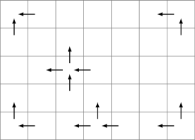
Figure 1: Visualisation of the reordering scheme for the pixels of the image. Arrows depict to which pixels the different terms are reassigned.

It follows now that (73) can be rewritten as

$$\frac{1}{h^{2}}\sum_{i=1}^{n_{p}}\left[\smashoperator[r]{\sum_{k\in\left\{i_{r}\right\}\cap N_{x}\left(i\right)}^{}}\left(u_{i}^{2}+u_{k}^{2}-2u_{i}u_{k}\right)\right.+\sum_{\mathclap{k\in\left\{i_{d}\right\}\cap N_{y}\left(i\right)}}\left(u_{i}^{2}+u_{k}^{2}-2u_{i}u_{k}\right)+\\ \hskip 28.45274pt\sum_{\mathclap{k\in\left\{i_{r}\right\}\cap N_{x}\left(i\right)}}\left(v_{i}^{2}+v_{k}^{2}-2v_{i}v_{k}\right)+\left.\sum_{\mathclap{k\in\left\{i_{d}\right\}\cap N_{y}\left(i\right)}}\left(v_{i}^{2}+v_{k}^{2}-2v_{i}v_{k}\right)\right]$$ (74)

which is obviously always nonnegative. By applying a similar reasoning as in mm04 , we see that (74) is $0$ if and only if $u_{i}=\text{const}_{u}$ and $v_{i}=\text{const}_{v}$ for all $i$. But then, it follows from (72) that $\left(f_{x}u+f_{y}v\right)^{2}_{i}=0$ can only be verified for all $i$ if and only if the spatial gradient $\nabla f$ is perpendicular to the flow field $\left(u,v\right)$. In particular, it has to be constant as well. On the other hand, $\nabla f$ is also perpendicular to the level curves $L_{c}\coloneqq\left\{x\ \middle|\ f\left(x,t\right)=c\right\}$. This implies, that the flow field must be tangent to $L_{c}$ at every point. All in all, this would mean that in the continuous setting the graph of $f$ would have to be a plane in $\mathbb{R}^{3}$ for all times $t$. Thus, if we exclude this case, where the graph is a plane, then the system matrix that we obtain in our Bregman iterations is always positive definite.

The above argumentation also holds if we only consider the grey value constancy, i.e. $\gamma=0$. On the other hand, the grey value constancy cannot be removed. If we only considered the constancy of the gradient, then the matrix is not necessarily positive definite. This concludes the proof.

7 Supplemental Numerical Experiments

The goal of this chapter will be to demonstrate the applicability of the Bregman framework by testing some of our algorithms on a certain number of image sequences. We will use two exemplary data sets from the Middlebury computer vision page middlebury . The correct ground truth of these sequences is known; therefore, it allows us to present an accurate evaluation of our algorithms. In order to give a quantitative representation of the accuracy of the obtained flow fields, we will consider the so called average angular error given by

$$\text{AAE}\left(u_{e},u_{c}\right)\coloneqq\frac{1}{n_{p}}\sum_{i,j}\arccos{\left(\frac{\langle{u_{c}}_{i,j},{u_{e}}_{i,j}\rangle}{\left\|{u_{c}}_{i,j}\right\|_{2}\left\|{u_{e}}_{i,j}\right\|_{2}}\right)}$$ (75)

as well as the average endpoint error defined as

$$\text{AEE}\left(u_{e},u_{c}\right)\coloneqq\frac{1}{n_{p}}\sum_{i,j}\left\|{u_{c}}_{i,j}-{u_{e}}_{i,j}\right\|_{2}$$ (76)

The subscripts $c$ and $e$ denote the correct respectively the estimated spatio-temporal optic flow vectors $u_{c}=\left(u_{c1},u_{c2},1\right)^{T}$ and $u_{e}=\left(u_{e1},u_{e2},1\right)^{T}$. In this context $n_{p}$ denotes the number of pixels of an image from the considered sequence. As for the qualitative evaluation of the computed flow fields, we will use the colour representation shown in Fig. 2. Here, the hue encodes the direction and the brightness represents the magnitude of the vector.

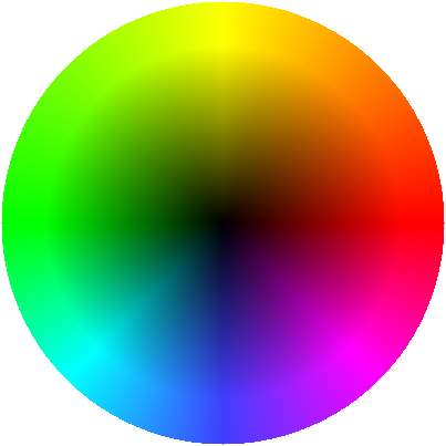
Figure 2: Color code for the displacement field.

In the following we will use the sequences depicted in Fig. 3 to test our algorithms.

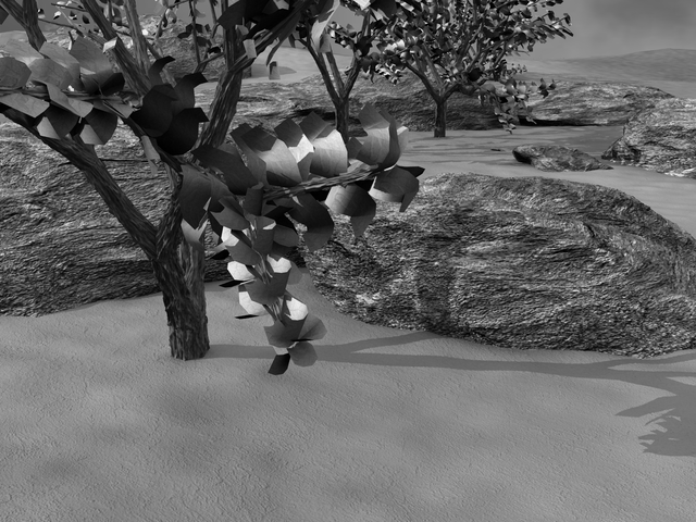
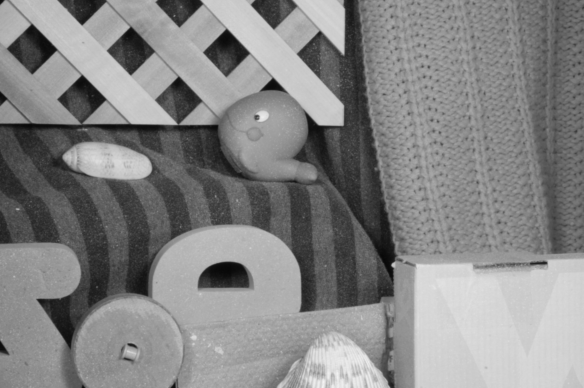
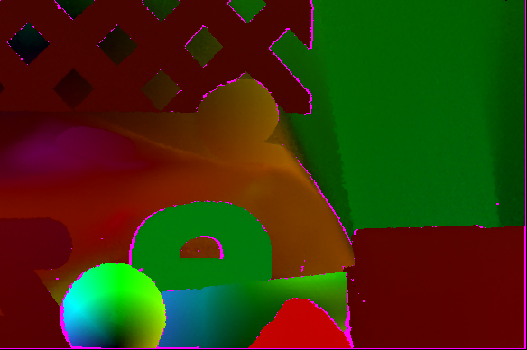
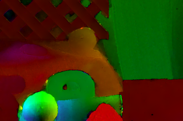
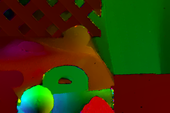
Figure 3: Top row: The considered image sequences with their corresponding ground truths. From left to right: Grove 2 frame 10, Grove 2 ground truth, Rubberwhale frame 10, Rubberwhale ground truth Bottom row: The obtained solutions with SBM. From left to right: Brox et al. model, OSB model, Brox et al. model, OSB model

The tests were done with the OSB model and the Brox et al. model. The occurring linear system was always solved with a simple Gauß-Seidel algorithm. Usually a few dozens of iterations were more than sufficient. The number of Bregman iterations for each model was chosen in such a way that the algorithm reached convergence for every considered sequence.

Figure 3 depicts the obtained flow fields and the Table 3 presents the parameter choices as well as the error measures and run times for the different algorithms. In this context RT denotes the run time in seconds. The meanings of the parameters $\lambda$, $\mu$ and $\gamma$ are the same as in the descriptions of the algorithms. $\sigma$ is the standard deviation used for the preprocessing of the images with a Gaussian convolution.

By looking at the results, we see that the OSB model is not only faster but also returns the more accurate flow fields. This behaviour confirms our previous concerns on the strong decoupling of the variables.

Table 3: Parameter choices and errors for the OSB model with 30 Bregman iterations, 10 Gauß-Seidel iterations and 3 alternating minimisations (first two rows) as well as 150 Bregman iterations, 10 Gauß-Seidel iterations and 3 alternating minimisations (last two rows).

Sequence	$\lambda$	$\mu$	$\gamma$	$\sigma$	AAE	AEE	RT
Rubberwhale	0.0100	11.25	20.00	0.40	4.06	0.12	93
Grove 2	0.0250	6.30	1.50	0.75	2.79	0.18	125
Rubberwhale	0.0065	0.23	1.00	0.38	4.67	0.14	530
Grove 2	0.0650	0.41	1.00	0.90	2.95	0.20	720

8 Conclusion

In this paper we have given an unified presentation of results on the Bregman iteration that were derived from several authors in different contexts and theoretical setups. Doing this, we have pointed out some relationships between actual results in that field, and we have also added some new details to the current state.

Furthermore, we have seen how the split Bregman algorithm can be applied to optical flow problems. We have presented two models based on variational formulations and showed how they can be discretised and solved with the split Bregman algorithm. We also discussed possible algorithmical improvements like occlusion handling and coarse-to-fine strategies that can easily be integrated into the Bregman framework.

As we could see, the formulations of all the presented algorithms are very similar. One Bregman iteration always consists in solving linear systems and applying thresholding operations. Not only are these algorithms easy to implement, they also offer themselves quite well for parallelisation. The occurring linear system can be solved with Jacobi iterations, which are well suited for massively parallel architectures such as GPUs. The shrinkage operations are also carried out componentwise and are equally suitable for parallel processing.

Finally, the positive definiteness of the system matrix allows us to consider a broad range of highly efficient algorithms for solving the occurring linear systems.

Our work is an example for a mathematical validation of important fundamental problems in computer vision. In the future we strive to provide further contributions in this field. Potential extensions of this work could include anisotropic regularisers for the herein presented approaches as well as further applications of the Bregman framework to computer vision tasks.

References

- [1] G. Aubert and P. Kornprobst. Mathematical problems in image processing, partial differential equations and the calculus of variations, volume 147 of Applied Mathematical Sciences. Springer, 2nd edition, 2006.
- [2] H. H. Bauschke and J. M. Borwein. Legendre functions and the method of random Bregman projections. Journal of Convex Analysis, 4(1):27–67, 1997.
- [3] R. Ben-Ari and N. Sochen. Variational stereo vision with sharp discontinuities and occlusion handling. In Proc. 2007 IEEE International Conference on Computer Vision, Rio de Janeiro, Brazil, 2007. IEEE Computer Society Press.
- [4] M. Black and P. Anandan. The robust estimation of multiple motions: parametric and piecewise smooth flow fields. Computer Vision and Image Understanding, 63(1):75–104, 1996.
- [5] A. Brandt. Multi-level adaptive technique (MLAT) for fast numerical solutions to boundary value problems. In H. Cabannes and R. Temam, editors, Proc. 3rd International Conference on Numerical Methods in Fluid Mechanics, volume 18 of Lecture Notes in Physics, pages 82–89, 1973.
- [6] A. Brandt and O. E. Livne. Multigrid Techniques, 1984 Guide with Applications to Fluid Dynamics. Classics in Applied Mathematics. SIAM, 2011.
- [7] L. M. Bregman. The relaxation method of finding the common point of convex sets and its application to the solution of problems in convex programming. USSR Computational Mathematics and Mathematical Physics, 7(3):200–217, 1967.
- [8] M. Breuß, H. Zimmer, and J. Weickert. Can variational models for correspondence problems benefit from upwind discretisations? Journal of Mathematical Imaging and Vision, 39(3):230–244, 2011.
- [9] W. L. Briggs, V. E. Henson, and S. F. McCormick. A Multigrid Tutorial. SIAM, 2nd edition, 2000.
- [10] T. Brox, A. Bruhn, N. Papenberg, and J. Weickert. High accuracy optical flow estimation based on a theory for warping. In T. Pajdla and J. Matas, editors, Computer Vision – ECCV 2004, Part IV, volume 3024 of LNCS, pages 25–36. Springer, 2004.
- [11] A. Bruhn. Variationelle Optische Flussberechnung Präzise Modellierung und effiziente Numerik. PhD thesis, Saarland University, 2006.
- [12] C. Brune, A. Sawatzky, and M. Burger. Primal and dual Bregman methods with application to optical nanoscopy. International Journal of Computer Vision, 92(2):211–229, 2011.
- [13] M. Burger, G. Gilboa, S. Osher, and J. Xu. Nonlinear inverse scale space methods. Communications in Mathematical Sciences, 4(1):175–208, 2006.
- [14] M. Burger, S. Osher, J. Xu, and G. Gilboa. Nonlinear inverse scale space methods for image restoration. In N. Paragios, O. D. Faugeras, T. Chan, and C. Schnörr, editors, Variational, Geometric, and Level Set Methods in Computer Vision (VLSM). Third international workshop, volume 3752 of LNCS, pages 25–36, Beijing, China, October 2005. Springer.
- [15] M. Burger, E. Resmerita, and L. He. Error estimation for Bregman iterations and inverse scale space methods. Computing, 81(2–3):109–135, 2007.
- [16] J.-F. Cai, S. Osher, and Z. Shen. Linearized Bregman iterations for compressed sensing. Mathematics of Computation, 78(267):1515–1536, 2009.
- [17] J.-F. Cai, S. Osher, and Z. Shen. Split Bregman methods and frame based image restoration. Multiscale Modeling & Simulation, 8(2):337–369, 2009.
- [18] A. Chambolle and T. Pock. A first-order primal-dual algorithm for convex problems with applications to imaging. Journal of Mathematical Imaging and Vision, 40:120–145, 2011.
- [19] T. F. Chan and P. Mulet. On the convergence of the lagged diffusivity fixed point method in total variation image restoration. SIAM Journal on Numerical Analysis, 36(2):354–367, 1999.
- [20] S. Cochran and G. Medioni. 3-D surface description from binocular stereo. IEEE Transactions on Pattern Analysis and Machine Intelligence, 14(10):981–994, 1992.
- [21] A. Dosovitskiy, P. Fischer, E. Ilg, P. Häusser, C. Hazirbas, V. Golkov, P. van der Smagt, D. Cremers, and T. Brox. Flownet: Learning optical flow with convolutional networks. In IEEE International Conference on Computer Vision (ICCV), 2015.
- [22] I. Ekeland and R. Téman. Convex analysis and variational problems. Number 28 in Classics in Applied Mathematics. Society for Industrial and Applied Mathematics, 1st edition, 1999.
- [23] E. Esser. Applications of lagrangian-based alternating direction methods and connections to split bregman. Computational and Applied Mathematics Reports cam09-31, University of California, 2009.
- [24] S. Fuc̆ik, A. Kratochvil, and J. Nec̆as. Kac̆anov–Galerkin method. Commentationes Mathematicae Universitatis Carolinae, 14(4):651–659, 1973.
- [25] P. Giselsson. Tight global linear convergence rate bounds for douglas-rachford splitting. Arxiv Technical Report 1506.01556v3, Lund University, 2016.
- [26] P. Giselsson and S. Boyd. Linear convergence and metric selection for douglas-rachford splitting and ADMM. IEEE Transactions on Automatic Control, 2016.
- [27] T. Goldstein, M. Li, and X. Yuan. Adaptive primal-dual splitting methods for statistical learning and image processing. In C. Cortes, N. D. Lawrence, D. D. Lee, M. Sugiyama, and R. Garnett, editors, Advances in Neural Information Processing Systems 28, pages 2089–2097. Curran Associates, Inc., 2015.
- [28] T. Goldstein and S. Osher. The split Bregman method for regularized problems. SIAM Journal on Imaging Sciences, 2(2):323–343, 2009.
- [29] W. Hackbusch. Multigrid Methods and Applications. Springer, 1985.
- [30] L. He, T.-C. Chang, S. Osher, T. Fang, and P. Speier. MR image reconstruction by using the iterative refinement method and nonlinear inverse scale space methods. UCLA CAM Report 06-35, University of California, Los Angeles, 2006.
- [31] L. Hoeltgen. Bregman iteration for optical flow. Master’s thesis, Saarland University, Saarbrücken, 2010.
- [32] L. Hoeltgen, S. Setzer, and M. Breuß. Intermediate flow field filtering in energy based optic flow computations. In Y. Boykov, F. Kahl, V. Lempitsky, and F. R. Schmidt, editors, Energy Minimization Methods in Computer Vision and Pattern Recognition, volume 6819 of LNCS, pages 315–328. Springer, 2011.
- [33] B. K. Horn and B. G. Schunck. Determining optical flow. Artificial Intelligence, 17(1–3):185–203, 1981.
- [34] Y. Kameda, A. Imiya, and N. Ohnishi. A convergence proof for the horn-schunck optical-flow computation scheme using neighborhood decomposition. In V. E. Brimkov, R. P. Barneva, and H. A. Hauptman, editors, Proceedings of the 12th international conference on Combinatorial image analysis, volume 4958 of LNCS, pages 262–273, Buffalo, USA, April 2008. Springer.
- [35] J. Kac̆ur, J. Nec̆as, J. Polák, and J. Souc̆ek. Convergence of a method for solving the magnetostatic field in nonlinear media. Aplikace Matematiky, 13:456–465, 1968.
- [36] C. Kirisits, L. F. Lang, and O. Scherzer. Optical flow on evolving surfaces with space and time regularisation. Journal of Mathematical Imaging and Vision, 52(1):55–70, 2015.
- [37] R. Klette, K. Schlüns, and A. Koschan. Computer Vision: Three-Dimensional Data from Images. Springer, 1998.
- [38] J. Lellmann, D. Breitenreicher, and C. Schnörr. Fast and exact primal-dual iterations for variational problems in computer vision. In K. Daniilidis, P. Maragos, and N. Paragios, editors, Computer Vision – ECCV 2010, volume 6312 of LNCS, pages 494–505. Springer Berlin Heidelberg, 2010.
- [39] A. Mansouri, A. Mitiche, and J. Konrad. Selective image diffusion: application to disparity estimation. In Proc. 1998 IEEE International Conference on Image Processing, volume 3, pages 284–288, Chicago, IL, 1998.
- [40] D. Maurer, Y. C. Ju, M. Breuß, and A. Bruhn. An efficient linearisation approach for variational perspective shape from shading. In Proc. German Conference on Pattern Recognition (GCPR), LNCS, pages 249–261. Springer, 2015.
- [41] A. Mitiche and A.-R. Mansouri. On convergence of the Horn and Schunck optical-flow estimation method. IEEE Transactions on Image Processing, 13(6):848–852, 2004.
- [42] E. Ménim and P. Pérez. Hierarchical estimation and segmentation of dense motion fields. International Journal of Computer Vision, 46(2):129–155, 2002.
- [43] H. Nien and J. A. Fessler. A convergence proof of the split Bregman method for regularized least-squares problems. Arxiv Technical Report 1402.4371v1, University of Michigan, 2014.
- [44] T. Nir, A. M. Bruckstein, and R. Kimmel. Over-parameterized variational optical flow. International Journal of Computer Vision, 76(2):205–216, 2008.
- [45] P. Ochs, T. Brox, and T. Pock. iPiasco: Inertial proximal algorithm for strongly convex optimization. Journal of Mathematical Imaging and Vision, 53:171–181, 2015.
- [46] P. Ochs, Y. Chen, T. Brox, and T. Pock. iPiano: Inertial proximal algorithm for non-convex optimization. SIAM Journal on Imaging Sciences, 7(2):1388–1419, 2014.
- [47] P. Ochs, A. Dosovitskiy, T. Brox, and T. Pock. On iteratively reweighted algorithms for nonsmooth nonconvex optimization in computer vision. SIAM J. Imaging Sci., 8(1):331–372, 2015.
- [48] S. Osher, M. Burger, D. Goldfarb, J. Xu, and W. Yin. An iterative regularization method for total variation-based image restoration. Multiscale Modeling and Simulation, 4(2):460–489, 2005.
- [49] S. Osher, Y. Mao, B. Dong, and W. Yin. Fast linearized Bregman iteration for compressive sensing and sparse denoising. Communications in Mathematical Sciences, 8(1):93–111, 2010.
- [50] T. Pock. Fast total variation for computer vision. PhD thesis, Graz University of Technology, 2008.
- [51] M. Proesmans, L. V. Gool, E. Pauwels, and A. Oosterlinck. Determination of optical flow and its discontinuities using non-linear diffusion. In J.-O. Eklundh, editor, Computer Vision – ECCV ’94, volume 801 of LNCS, pages 295–304. Springer, 1994.
- [52] R. T. Rockafellar. Convex analysis. Princeton Landmarks in Mathematics and Physics. Princeton University Press, 10th edition, 1997.
- [53] R. T. Rockafellar and J.-B. Wets. Variational Analysis, volume 317 of A series of comprehensive studies in mathematics. Springer, 1st edition, 1998.
- [54] L. I. Rudin, S. Osher, and E. Fatemi. Nonlinear total variation based noise removal algorithms. Physica D: Nonlinear Phenomena, 60(1–4):259–268, 1992.
- [55] D. Scharstein and R. Szeliski. The middlebury computer vision pages. Online.
- [56] S. Setzer. Split Bregman algorithm, Douglas-Rachford splitting and frame shrinkage. In X.-C. Tai, K. Mørken, M. Lysaker, and K.-A. Lie, editors, Scale Space and Variational Methods in Computer Vision, volume 5567 of LNCS, pages 464–476, Voss, Norway, June 2009. Springer.
- [57] N. Slesareva, A. Bruhn, and J. Weickert. Optic flow goes stereo: A variational method for estimating discontinuity-preserving dense disparity maps. In W. Kropatsch, R. Sablatnig, and A. Hanbury, editors, Pattern Recognition, volume 3663 of LNCS, pages 33–40. Springer, 2005.
- [58] D. Sun, S. Roth, J. P. Lewis, and M. J. Black. Learning optical flow. In D. Forsyth, P. Torr, and A. Zisserman, editors, Computer Vision - ECCV 2008, volume 5304 of LNCS, pages 83–97. Springer Berlin Heidelberg, 2008.
- [59] E. Trucco and A. Verri. Introductory Techniques for 3-D Computer Vision. Prentice Hall, Englewood Cliffs, 1998.
- [60] A. Wedel, D. Cremers, T. Pock, and H. Bischof. Structure- and motion-adaptive regularization for high accuracy optic flow. In Proc. 2009 IEEE International Conference on Computer Vision, Kyoto, Japan, 2009. IEEE Computer Society Press.
- [61] A. Wedel, T. Pock, C. Zach, H. Bischof, and D. Cremers. An improved algorithm for TV– optical flow computation. In D. Cremers, B. Rosenhahn, A. L. Yuille, and F. R. Schmidt, editors, Statistical and Geometrical Approaches to Visual Motion Analysis, volume 5604 of LNCS, pages 23–45. Springer, 2008.
- [62] J. Weickert, A. Bruhn, T. Brox, and N. Papenberg. Mathematical Models for Registration and Applications to Medical Imaging, chapter A Survey on Variational Optic Flow Methods for Small Displacements, pages 103–136. Mathematics in Industry. Springer, 2006.
- [63] J. Weickert, A. Bruhn, N. Papenberg, and T. Brox. Variational optic flow computation: From continuous models to algorithms. In L. Alvarez, editor, IWCVIA ’03: International Workshop on Computer Vision and Image Analysis, volume 0026, pages 1–6, Spain, 2004. Cuadernos del Instituto Universitario de Ciencias y Tecnologias Ciberneticas, University of Las Palmas de Gran Canaria.
- [64] P. Weinzaepfel, J. Revaud, Z. Harchaoui, and C. Schmid. Deepflow: Large displacement optical flow with deep matching. In ICCV 2013 - IEEE Intenational Conference on Computer Vision, 2013.
- [65] M. Werlberger, T. Pock, and H. Bischof. Motion estimation with non-local total variation regularization. In Proc. 2010 IEEE Computer Society Conference on Computer Vision and Pattern Recognition, San Francisco, CA, USA, 2010. IEEE Computer Society Press.
- [66] P. Wesseling. An Introduction to Multigrid Methods. Wiley, 1992.
- [67] J. Xu and S. Osher. Iterative regularization and nonlinear inverse scale space applied to wavelet-based denoising. IEEE Transactions on Image Processing, 16(2):534–544, 2006.
- [68] L. Xu, J. Jia, and Y. Matsushita. Motion detail preserving optical flow estimation. In Proc. 2010 IEEE Computer Society Conference on Computer Vision and Pattern Recognition, San Francisco, CA, USA, 2010. IEEE Computer Society Press.
- [69] Y. Yang, M. Möller, and S. Osher. A dual split Bregman method for fast minimization. Mathematics of Computation, 82:2061–2085, 2013.
- [70] W. Yin and S. Osher. Error forgetting of Bregman iteration. Journal of Scientific Computing, 54(2):684–695, 2013.
- [71] W. Yin, S. Osher, D. Goldfarb, and J. Darbon. Bregman iterative algorithms for l1-minimization with applications to compressed sensing. SIAM Journal on Imaging Sciences, 1(1):143–168, 2007.
- [72] C. Zach, T. Pock, and B. Horst. A duality based approach for realtime TV–L1 optical flow. In F. A. Hamprecht, C. Schnörr, and B. Jähne, editors, Proceedings of the 29th DAGM Symposium on Pattern Recognition, volume 4713 of LNCS, pages 214–223, Heidelberg, Germany, September 2007. Springer.
- [73] X. Zhang, M. Burger, X. Bresson, and S. Osher. Bregmanized nonlocal regularization for deconvolution and sparse reconstruction. UCLA CAM Report 09-03, University of California, Los Angeles, 2009.
- [74] H. Zimmer, M. Breuß, J. Weickert, and H.-P. Seidel. Hyperbolic numerics for variational approaches to correspondence problems. In X.-C. T. et al., editor, Scale-Space and Variational Methods in Computer Vision, volume 5567 of LNCS, pages 636–647. Springer, Berlin, 2009.
- [75] H. Zimmer, A. Bruhn, and J. Weickert. Optic flow in harmony. International Journal of Computer Vision, 93(3):368–388, 2011.
- [76] H. Zimmer, A. Bruhn, J. Weickert, L. Valgaerts, A. Salgado, B. Rosenhahn, and H.-P. Seidel. Complementary optic flow. In D. Cremers, Y. Boykov, A. Blake, and F. R. Schmidt, editors, Energy Minimization Methods in Computer Vision and Pattern Recognition (EMMCVPR), volume 5681 of Lecture notes in computer science, pages 207–220. Springer, 2009.