Delocalization of two interacting particles in the two-dimensional Harper model

Abstract

We study the problem of two interacting particles in a two-dimensional quasiperiodic potential of the Harper model. We consider an amplitude of the quasiperiodic potential such that in absence of interactions all eigenstates are exponentially localized while the two interacting particles are delocalized showing anomalous subdiffusive spreading over the lattice with the spreading exponent $b\approx 0.5$ instead of a usual diffusion with $b=1$. This spreading is stronger than in the case of a correlated disorder potential with a one particle localization length as for the quasiperiodic potential. At the same time we do not find signatures of ballistic FIKS pairs existing for two interacting particles in the one-dimensional Harper model.

1 Introduction

The Harper problem describes the quantum dynamics of an electron in a two-dimensional potential (2D) in a perpendicular magnetic field harper . It can be reduced to the Schrödinger equation on a discrete quasiperiodic one-dimensional (1D) lattice. This system has fractal spectral properties hofstadter and demonstrates a Metal-Insulator Transition (MIT), established by Aubry and André aubry . The MIT takes place when the amplitude $\lambda$ of the quasiperiodic potential (with hopping being unity) is changed from $\lambda<2$ (metallic phase) to $\lambda>2$ (insulator phase). A review of the properties of the Aubry-André model can be found in sokoloff and the mathematical prove of the MIT is given in lana1 .

The investigation of interaction effects between particles in the 1D Harper model was started in dlsharper with the case of Two Interacting Particles (TIP). It was found that the Hubbard interaction can create TIP localized states in the noninteracting metallic phase. Further studies also demonstrated the localization effects in presence of interactions barelli ; orso . This trend was opposite to the TIP effect in disordered systems where the interactions increase the TIP localization length in 1D or even lead to delocalization of TIP pairs for dimensions $d\geq 2$ dlstip ; imry ; pichard ; frahm1995 ; vonoppen ; borgonovi ; dlsmoriond ; frahmtip ; dlscoulomb ; lagesring .

Thus the results obtained in flach on the appearance of delocalized TIP pairs in the 1D Harper model, for certain particular values of interaction strength and energy, in the regime, when all one-particle states are exponentially localized, is really striking. In flach the delocalization of TIP appears at a relatively strong interaction being the reason why this effect was missed in previous studies. The recent advanced analysis fiks1d showed that so called Freed by Interaction Kinetic States (FIKS) appear at various irrational magnetic flux values being ballistic or quasi-ballistic over the whole system size $N$ used in numerical simulations (up to $N=10946$). At certain flux values the FIKS pairs appear even at a moderate Hubbard interaction $U=1.75$ (hopping is taken as $t=1$), also the effect of FIKS pairs becomes stronger for long range interactions fiks1d . Up to 12% from an initial state, with TIP being close to each other, can be projected on the FIKS pairs escaping ballistically to infinity fiks1d . This observation points to possible significant applications of FIKS pairs in various physical systems and shows the importance of further investigations of the FIKS effect. Indeed, as shown in fiks1d , the recent experiments with cold atoms on quasiperiodic lattices roati ; modugno ; bloch should be able to detect FIKS pairs in 1D.

For the TIP effect in disordered systems the dimension plays an important role imry ; borgonovi ; dlsmoriond ; dlscoulomb ; lagesring and it is clear that it is important to study the FIKS effect in higher dimensions. We start these investigations here for the two-dimensional (2D) Harper model where the (noninteracting) eigenstates are given by the product of two 1D Harper (noninteracting) eigenstates so that the MIT position for noninteracting states is clearly defined at $\lambda=2$. We note that 2D quasiperiodic lattices of cold atoms have been realized in recent experiments (even if the second dimension was a repetition of 1D lattices) bloch2d so that there are new possibilities to investigate the FIKS effect with cold atoms when the interaction is taken into account.

The paper is composed as follows: the model description is given in Section 2, the main results are presented in Section 3, discussion of results is given in Section 4. High resolution figures and additional data are available at the web site webpage .

2 Model description

We consider particles in a 2D lattice of size $N_{1}\times N_{2}$, $0\leq x<\!N_{1}$ and $0\leq y<\!N_{2}$. The one-particle Hamiltonian $h^{(j)}$ for particle $j$ is given by:

$$h^{(j)} = T^{(j)}+V^{(j)},$$ (1)

$$T^{(j)} = -\sum_{x,y}\Bigl{(}|x,y\!>_{j}\,<\!x+1,y|_{j}$$

$$\qquad\quad+|x,y\!>_{j}\,<\!x,y+1|_{j}\Bigr{)}+h.~{}c.,$$

$$V^{(j)} = \sum_{x,y}\Bigl{[}V_{1}(x-x_{0})+V_{2}(y-y_{0})\Bigr{]}|x,y\!>_{j}\,<\!x,y|_{j}.$$ (3)

The point $(x_{0},y_{0})=(N_{1}/2,N_{2}/2)$ is the “center point” of the lattice and the offsets $x-x_{0}$ or $y-y_{0}$ in the arguments of $V_{1}$ ensure that the potential has locally the same structure for the region close to the center point when varying the system size $N_{1}\times N_{2}$. The kinetic energy $T^{(j)}$ is given by the standard tight-binding model in two dimensions with hopping elements $t=-1$ linking nearest neighbor sites with periodic boundary conditions, i. e. $x+1$ (or $y+1$) in (2) is taken modulo $N_{1}$ (or $N_{2}$). Note that the potential is of the form

$$V(x,y)=V_{1}(x-x_{0})+V_{1}(y-y_{0})$$ (4)

where $V_{1}(x)$, $V_{2}(y)$ are effective one-dimensional potentials. In this work we study essentially the quasiperiodic case with $V_{1}(x)=\lambda_{x}\cos(\alpha x+\beta)$, $V_{2}(y)=\lambda_{y}\cos(\alpha y+\beta)$ and here mostly $\lambda_{x}=\lambda_{y}=\lambda=2.5$. Furthermore we choose $\alpha=2\pi(\sqrt{5}-1)/2\approx 0.61803$ as the golden ratio and $\beta=1/\sqrt{2}$. For these parameters the one-dimensional eigenfunctions (with the $V_{1}$ potential) are localized with a one-dimensional localization length $\ell=1/\log(\lambda/2)\approx 4.48$ (see e.g. sokoloff ; fiks1d ). For the purpose of comparison we also study the disorder case with a random potential $V_{1}(x)$ uniformly distributed in $[-W/2,W/2]$ and the same random realization for $V_{2}(y)$. For this case we choose $W=5$ corresponding to the localization length $\ell\approx 105/W^{2}\approx 4.2$ which is quite close to the localization length of the quasiperiodic case for $\lambda=2.5$. The particular structure of $V$ implies that for both cases the eigenfunctions of $h^{(j)}$ are products of one-dimensional localized eigenstates in $x$ and $y$ with the potential $V_{1}(x-x_{0})$ or $V_{2}(y-y_{0})$.

We note that for the disorder case the potential $V(x,y)$ is due to the particular sum structure in Eq. (3) very different from the standard Anderson two-dimensional disorder model. In the latter case $V(x,y)$ would be independent random variables for each value of $(x,y)$ while in our case $V(x,y)$ is a sum of two one-dimensional disorder potentials providing certain spacial correlations in the potential which are crucial for the value of the quite small localization length.

We now consider two interacting particles, each of them submitted to the one-particle Hamiltonian $h^{(j)}$, and coupled by an interaction potential $U(x_{1},y_{1},x_{2},y_{2})$ which has a non-vanishing value $U$ only for $|x_{1}-x_{2}|<\!U_{R}$ and $|y_{1}-y_{2}|<\!U_{R}$ U_boundary . Here $U$ denotes the interaction strength and $U_{R}$ is the interaction range. The total two particle Hamiltonian is given by

$$H=h^{(1)}+h^{(2)}+\hat{U}$$ (5)

where $\hat{U}$ is the interaction operator in the two-particle Hilbert space with diagonal entries $U(x_{1},y_{1},x_{2},y_{2})$. In this work we consider two cases with $U_{R}=1$, corresponding to Hubbard on-site-interaction, and $U_{R}=2$ corresponding to a short range interaction with 9 neighboring sites coupled by the interaction.

The eigenfunctions of $H$ are either symmetric with respect to particle permutation (boson case) or anti-symmetric (fermion case) corresponding to a decomposition of the Hilbert space in a boson- and fermion-subspace. However, in this work we prefer to work on the complete space (of dimension $N_{1}^{2}\,N_{2}^{2}$) due to the employed numerical method to determine the time evolution of the wave function. The evolution is described by the time-dependent Schrödinger equation (with $\hbar=1$)

$$i\frac{\partial}{\partial t}\,|\psi(t)\!>=H\,|\psi(t)\!>.$$ (6)

The symmetry of the state $|\psi(t)\!>$ is simply fixed by the symmetry of the initial condition which is conserved by the Schrödinger equation and which we choose

$$|\psi(0)\!>=|x_{0},y_{0}\!>_{1}\,|x_{0},y_{0}\!>_{2}$$ (7)

corresponding to both particles being localized on the same center point with $x_{0}=N_{1}/2$ and $y_{0}=N_{2}/2$.

As already noted, in absence of the interaction, i. e. $U=0$, the eigenstates are localized with a typical localization length $\ell$ (in each direction). Thus, our aim is to study if interaction leads to a delocalization of TIP during the time evolution or to some kind of diffusion of TIP in coordinate or Hilbert space.

To solve (6) numerically we write $H=H_{x}+H_{p}$ as a sum of two parts which are either diagonal in position space $H_{x}=V^{(1)}+V^{(2)}+\hat{U}$ or in momentum space $H_{p}=T^{(1)}+T^{(2)}$ and evaluate the solution of (6) as:

$$|\psi(t)\!>=\exp(-iHt)\,|\psi(0)\!>$$ (8)

using the Trotter formula approximation:

$$\exp(-iHt) \approx (O_{p}\,O_{x})^{t/\Delta t},$$ (9)

$$O_{p} = \exp(-iH_{p}\,\Delta t),\quad O_{x}=\exp(-iH_{x}\,\Delta t)$$

with two unitary operators $O_{p}$ and $O_{x}$. The integration time step $\Delta t$ is supposed to be small as compared to typical inverse energy scales and the value of $t$ is chosen such that $t/\Delta t$ is integer. Formally, Eq. (9) becomes exact in the limit $\Delta t\to 0$. However, a finite value of $\Delta t$ implies a modification of the Hamiltonian with $H\to\tilde{H}$ with $\tilde{H}$ defined by $O_{p}\,O_{x}=\exp(-i\tilde{H}\,\Delta t)$ and related to $H$ by a power law expansion in $\Delta t$ where the corrections are given as (higher order) commutators between $H_{x}$ and $H_{p}$. In this work we choose the value $\Delta t=0.1$ but we have verified for certain parameter values that the results presented below do not change significantly if compared with $\Delta t=0.05$. The efficiency and stability of this type of integration methods have been demonstrated in dlstip ; fiks1d ; danse ; garcia .

The operators $O_{x}$ and $O_{p}$ are either diagonal in position representation or momentum representation. In order to evaluate (8) using (9) we first apply the operator $O_{x}$ to the initial state given in position representation which can be done efficiently with $N_{\rm tot}=N_{1}^{2}\,N_{2}^{2}$ operations by multiplying the eigenphases of $O_{x}$ to each component of the state. Then the state is transformed to momentum representation using a fast Fourier transform in the four dimensional configuration space (corresponding to two particles in two dimensions) with help of the library FFTW fftw which requires about $N_{\rm tot}(\log N_{1}+\log N_{2})$ operations. At this point we can efficiently apply the operator $O_{p}$ to the states, again by multiplying the eigenphases to each component of the state and finally we apply the inverse Fourier transform to come back in position representation. The eigenphases of $O_{x}$ and $O_{p}$ can be calculated and stored in advance.

We determine the time evolution of $|\psi(t)\!>$ using Eq. (9) for different square and rectangular geometries with system sizes up to $128\times 128$ (i. e. $N_{1}=N_{2}=128$) or $1024\times 8$ (i. e. $N_{1}=1024$, $N_{2}=8$). At $N_{1}=N_{2}=128$ the Hilbert space of the whole system becomes as large as $N_{H}=N_{1}^{4}\approx 2.7\times 10^{8}$. In order to analyze the structure of the TIP state we introduce different quantities and densities described below.

First let us denote by

$$\psi(x_{1},y_{1},x_{2},y_{2})=<\!x_{1},y_{1}|_{1}<\!x_{2},y_{2}|_{2}\,\psi\!>$$ (10)

the (non-symmetrized) two particle wave function and for simplicity we omit the argument for the time dependence. Then the one-particle density $\rho_{1}(x,y)$ in 2D is defined as

$$\rho_{1}(x,y)=\sum_{x_{2},y_{2}}|\psi(x,y,x_{2},y_{2})|^{2}.$$ (11)

We note that the normalization of the state $|\psi\!>$ implies $\sum_{x,y}\rho_{1}(x,y)=1$. Using this one-particle density we define the variance with respect to the center point $(x_{0},y_{0})$ by

$$\langle r^{2}\rangle=\sum_{x,y}\Bigl{[}(x-x_{0})^{2}+(y-y_{0})^{2}]\,\rho_{1}(x,y)$$ (12)

and also the inverse participation ratio (IPR) “without center” by:

$$\xi_{\rm IPR}=\frac{\left[\sum_{(x,y)\in S}\rho_{1}(x,y)\right]^{2}}{\sum_{(x,y)\in S}\rho_{1}^{2}(x,y)}$$ (13)

where the sums run over the set

$$S=\Bigl{\{}(x,y)\ \Big{|}\ |x-x_{0}|>N_{1}/10\ ,\ |y-y_{0}|>N_{2}/10\Bigr{\}}$$ (14)

containing only lattice sites $(x,y)$ outside the center rectangle of (linear) size 20% around the center point $(x_{0},y_{0})$. This kind of definition for the IPR allows to detect a particular kind of partial delocalization where only a small fraction of probability diffuses to large distances with respect to the center point while the remaining probability stays strongly localized close to the center point. This quantity was already used with success in our studies of FIKS pairs in fiks1d for the 1D TIP Harper problem. Using the standard definition for the IPR (where $S$ would be the set of all lattice sites) allows only to detect a strong delocalization of the full probability. For the variance $\langle r^{2}\rangle$ the contribution of the probability at the initial state is not so pronounced and thus we compute this quantity for the whole lattice.

We furthermore introduce the following densities

$$\rho_{x}(x) = \sum_{y}\rho_{1}(x,y),$$ (15)

$$\rho_{y}(y) = \sum_{x}\rho_{1}(x,y),$$ (16)

$$\rho_{xx}(x_{1},x_{2}) = \sum_{y_{1},y_{2}}|\psi(x_{1},y_{1},x_{2},y_{2})|^{2},$$ (17)

$$\rho_{\rm lin}(s) = \sum_{\scriptsize\begin{array}[]{c}x,y\\ s=|x-x_{0}|+|y-y_{0}|\\ \end{array}}\rho_{1}(x,y).$$ (20)

The density $\rho_{x}(x)$ (or $\rho_{y}(y)$) is simply the one-particle density integrated over the $y$-direction (or $x$-direction). $\rho_{xx}(x_{1},x_{2})$ is the two particle density integrated over both $y$-directions giving information about the spatial correlations of both particles in $x$-direction. Here $\rho_{\rm lin}(s)$ is the linear density obtained from the one-particle density by summing over all sites with same (1-norm)-distance $s=|x-x_{0}|+|y-y_{0}|$ from the center point and is well defined for $0\leq s<(N_{1}+N_{2})/2$. This density is similar in spirit to a radial density obtained by integrating over all points with the same distance from the center point. However, using the 1-norm (and not the Euclidean 2-norm) to measure the distance is both more convenient for the practical calculation and actually physically more relevant for the case where $\rho_{1}(x,y)\sim\exp[-(|x-x_{0}|+|y-y_{0}|)/l]=\exp(-s/l)$ is similar to a product of two exponentially localized functions in $x$ and $y$ with the same localization length $l$.

3 Time evolution results

As in fiks1d we first determine the most promising values of the interaction strength $U$ by computing $\langle r^{2}\rangle$ and $\xi_{\rm IPR}$ at a certain large $t$. Here we use a moderate system size since computations should be done for many values of $U$ at $U_{R}=1$ (Hubbard interaction) and $U_{R}=2$ (9 nearest sites coupled on a square lattice). The results are presented in Fig. 1. We see that there are regions of $U$ where the values of $\langle r^{2}\rangle$ are by a factor $4-10$ larger than in the case of $U=0$ where $\langle r^{2}\rangle\approx 10$ (see Fig. 2). However, in contrast to the 1D TIP Harper model fiks1d there are no sharp peaks in $U$ except maybe at $U=3.5$ for $U_{R}=2$. In the following, we choose this value for a more detailed analysis at larger sizes $N_{1},N_{2}$ and larger times $t$. However, we have also studied some other $U$ values, e. g. $U=6$ with qualitatively similar results but typically with less delocalization than the most interesting value $U=3.5$.

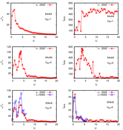
Figure 1: Variance $\langle r^{2}\rangle$ (left column) and IPR without center $\xi_{\rm IPR}$ (right column) versus interaction strength $U$ for $0\leq U<20$ for 2D quasiperiodic potential ($\lambda=2.5$). The top panels correspond to Hubbard interaction ($U_{R}=1$) and the square geometry $N_{1}=N_{2}=64$; the center panels correspond to $U_{R}=2$ for $N_{1}=N_{2}=64$; the bottom panels correspond to $U_{R}=2$ with rectangular geometry $N_{1}=256,\ N_{2}=8$. In all panels the iteration time is $t=2500$ except for the two bottom panels where additional data points for $t=10000$ and $0\leq U\leq 6.0$ are shown.

In Fig. 2, we show for $U=3.5$, the two values $U_{R}=1$ and $U_{R}=2$ and different geometries the time dependence of $\langle r^{2}\rangle$ and $\xi_{\rm IPR}$. All the cases with a square geometry $N_{1}=N_{2}$ show an unlimited growth of these two quantities up to largest times $t=10^{5}$ reached in our numerical simulations. For the Hubbard case at $U_{R}=1$ the system size is sufficiently large to avoid saturation effects due the finite system size and the change of size from $N_{1}=N_{2}=96$ to $128$ does not affect the values of $\langle r^{2}\rangle$ and $\xi_{\rm IPR}$ at $U=3.5$. For $U_{R}=2$ we have larger values of $\langle r^{2}\rangle$ and $\xi_{\rm IPR}$ and it is clear that the size $N_{1}=N_{2}=96$ is sufficiently large only up to $t\approx 10^{4}$ while for $N_{1}=N_{2}=128$ the size is sufficient only up to $t\approx 3\times 10^{4}$ with a finite size induced saturation of growth for $3\times 10^{4}<t\leq 10^{5}$.

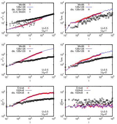
Figure 2: Variance $\langle r^{2}\rangle$ (left column) and IPR without center $\xi_{\rm IPR}$ (right column) versus iteration time $10\leq t\leq 10^{5}$ in a double logarithmic scale. The two top panels correspond to Hubbard interaction with interaction range $U_{R}=1$, the square geometry $N_{1}=N_{2}=128$ (blue curve) or $N_{1}=N_{2}=96$ (red crosses for $10\leq t\leq 10^{4}$). In the top left panel also data for $U=0$, $N_{1}=N_{2}=64$, $10\leq t\leq 2500$ (grey points) are shown. The two center panels correspond to $U_{R}=2$ and the same geometries as in the top panels. The two bottom panels correspond to $U_{R}=2$ with rectangular geometries $N_{1}=1024$, $N_{2}=8$ (blue curve) and $N_{1}=512$, $N_{2}=8$ (red crosses). Furthermore in all panels data for a random disorder potential ($W=5$) of the particular form (4) (see text) and same panel values $N_{1},N_{2}$ are shown by black squares. In all panels the interaction strength is $U=3.5$. All curves and symbols, except the black squares, correspond to the 2D Harper model at $\lambda=2.5$. The number of shown data points is artificially reduced to increase the visibility.

In a drastic contrast with the 1D case fiks1d we observe only a subdiffusive growth of $\langle r^{2}\rangle\propto t^{b_{1}}$ and $\xi_{\rm IPR}\propto t^{b_{2}}$ with time. The power law fits of the data used in Fig. 2 provide the values: $b_{1}=0.438\pm 0.004$, $b_{2}=0.503\pm 0.007$ for $U_{R}=1$; $b_{1}=0.521\pm 0.002$, $b_{2}=0.506\pm 0.009$ for $U_{R}=2$ for the range $100\leq t\leq 10^{5}$ at $N_{1}=N_{2}=128$.

For comparison, we also present in Fig. 2 the same quantities for the case of the particular disordered potential described in Section 2. For this we use the same interaction strength $U=3.5$ and the disorder parameter $W=5$ which gives approximately the same localization length in 1D as for the 1D Harper model at $\lambda=2.5$ (however, for the usual 2D Anderson model we would have a significantly larger value of the one-particle IPR $\xi\approx 150$, see e.g. Fig. 2 in lagesbls ). For $U_{R}=2$ and $t>10^{2}$ both the absolute values and the growth rates of $\langle r^{2}\rangle$ and $\xi_{\rm IPR}$ for the disorder case are significantly lower as compared to the 2D Harper model. For $U_{R}=1$ the disorder values of the variance are above the variance values of the 2D Harper model, for the time interval $10\leq t\leq 10^{5}$ shown in the figure, but the curve for the Harper case has a stronger growth rate (larger slope).

Actually, according to Fig. 2 the two curves for $\langle r^{2}\rangle$ seem to intersect at a certain time $t_{\rm int}$ and therefore we expect the variance of the 2D Harper model to become stronger than the variance of the disorder case for $t>t_{\rm int}$. From the figure it seems that $t_{\rm int}$ is close or slightly below $10^{5}$ but this is only due to the rather thick data points and the logarithmic scale. A careful analysis of the data (higher resolution figure and more precise extrapolation of both curves using power law fits for $10^{4}\leq t\leq 10^{5}$) shows that the intersection point is likely to be close to the value $t_{\rm int}\approx 2.4\times 10^{5}$. For $U_{R}=1$, the another quantity $\xi_{\rm IPR}$ for the disorder case is clearly below the curve of the Harper model. Our interpretation is that apparently for TIP in the disorder case there is a relative strong initial spreading at short times and a modest length scale but for a strong weight of the wave packet while for the Harper case there is a slower but long range delocalization for a smaller weight of the wavepacket which is better visible from the IPR $\xi_{\rm IPR}$ without the center rectangle. (This kind of “long range small weight” delocalization was also found for the FIKS pairs of the TIP 1D Harper model fiks1d but there the growth rate is actually ballistic, corresponding to power law exponents $b_{1,2}\approx 2$, and not sub-diffusive.)

The lower growth rate for the disorder case at both values of $U_{R}$ is also clearly confirmed by the power law fits which provide (for the same time and size ranges as for the Harper case) the exponents: $b_{1}=0.218\pm 0.005$, $b_{2}=0.404\pm 0.035$ for $U_{R}=1$ and $b_{1}=0.181\pm 0.007$, $b_{2}=0.302\pm 0.009$ for $U_{R}=2$.

In Fig. 2 we also consider the case of two rectangular geometries with $N_{1}=1024$ or $N_{1}=512$ and $N_{2}=8$. In this case there is a clear saturation of growth of the considered variables independent of the system size. These data show that for $N_{2}\sim\ell$ we have a localization of TIP in the quasi-1D Harper model at the considered interaction strength. However, this result does not exclude the possibility of appearance of FIKS pairs in the quasi-1D limit at other interaction values, even if our preliminary tests indicate similar localization results.

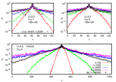
Figure 3: Density $\rho_{x}(x)$ versus $x$ in a semilogarithmic representation for different values of interaction range, geometry and iteration times at $U=3.5$. The color labels shown in the bottom right corner of the bottom panel apply to all three panels: $t=100$ (red curve), $t=1000$ (green curve), $t=10000$ (blue curve), $t=100000$ (pink curve), disorder potential ($W=5$) for $t=100000$ (black squares). In the top left panel also data for $U=0$, $N_{1}=N_{2}=64$, $t\leq 2500$ (grey points) are shown (with center point shifted from 32 to 64). All curves, except the black squares, correspond to the quasiperiodic potential ($\lambda=2.5$). For grey points and black squares the number of shown data points is artificially reduced to increase the visibility.

The time evolution of the projected one-particle probability distribution $\rho_{x}(x)$ is shown in Fig. 3. For the square geometry $N_{1}=N_{2}=128$ the width of the distribution is growing with time and it becomes practically flat at maximal times $t=10^{5}$ for both values $U_{R}=1$ or $U_{R}=2$. In the case of disorder we have also a significant spreading of probability over lattice sites which is somewhat comparable with those of the 2D Harper case. For the rectangular geometry we have a significantly larger probability on the tails for the 2D Harper model as compared to the disorder case. This is in agreement with the data for $\langle r^{2}\rangle$ in Fig. 2 (bottom left panel).

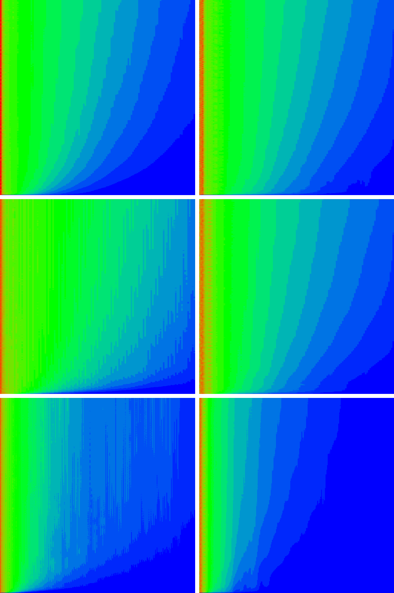
Figure 4: Density plot of the time evolution of the linear density $\rho_{\rm lin}(s)$. The vertical axis corresponds to the iteration time $0\leq t\leq 10000$ and the horizontal axis corresponds to $0\leq s<(N_{1}+N_{2})/2$. The left column corresponds to the quasiperiodic potential ($\lambda=2.5$) and the right column to the disorder case ($W=5$). All panels correspond to the interaction strength $U=3.5$. Top (center) panels correspond to $U_{R}=1$ ($U_{R}=2$) and the square geometry $N_{1}=N_{2}=128$. Bottom panels correspond to $U_{R}=2$ and the rectangular geometry $N_{1}=512$, $N_{2}=8$. The color codes of the density plot correspond to red for maximum, green for medium and blue for minimum values.

These results show that there are no ballistic type FIKS pairs propagating through the whole system as it was the case for TIP in the 1D Harper model flach ; fiks1d . Such a conclusion is confirmed by the analysis of the time evolution of the linear density $\rho_{\rm lin}(s)$ defined in (20) as shown in Fig. 4. The typical width of this density does not increase linearly in time in contrast to the 1D Harper case (see e.g. Fig. 3 in fiks1d ) and we have in Fig. 4 (for the square geometry cases) curves in the $(s,t)$-plane, corresponding to a subdiffusive spreading $\langle s^{2}\rangle\sim t^{b}$ with an exponent $b\sim 0.5$. For the disorder case (with square geometry) the corresponding curves of Fig. 4 are also in a qualitative agreement with the reduced exponent $b\sim 0.2$ found above by the fit of $\langle r^{2}\rangle$. Concerning the rectangular geometries the curves visible in Fig. 4 show saturation also in agreement with Fig. 2 even though for the quasiperiodic potential the tails of the distribution (visible by light blue zones) still continue to increase which is also quite in agreement with the bottom panel of Fig. 3.

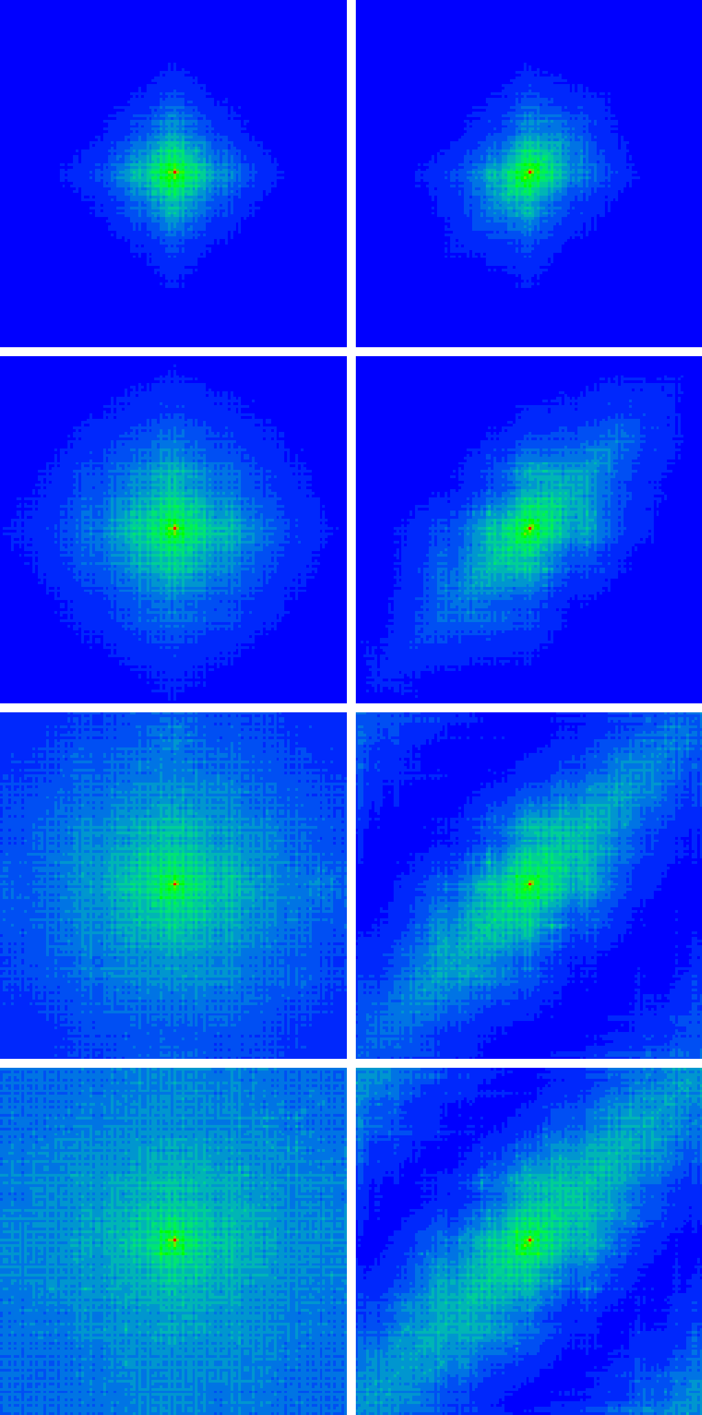
Figure 5: Density plot for the densities $\rho_{1}(x,y)$ (left column) and $\rho_{xx}(x_{1},x_{2})$ (right column) with $x$ (or $x_{1}$) for the horizontal axis and $y$ (or $x_{2}$) for the vertical axis. All panels correspond to $U=3.5$, $U_{R}=1$ and the square geometry $N_{1}=N_{2}=128$ with the quasiperiodic potential ($\lambda=2.5$). The different rows correspond to the iteration time $t=100$ (first row), $t=1000$ (second row), $t=10000$ (third row) and $t=100000$ (fourth row).

The one-particle density $\rho_{1}(x,y)$ for the square geometry $128\times 128$ and $U_{R}=1$ (or $U_{R}=2$) is shown at different moments of time in the left column of Fig. 5 (Fig. 7) for the 2D Harper case and of Fig. 6 (Fig. 8) for the disorder case. The relative distribution of TIP probability in the $(x_{1},x_{2})$-plane, i. e. the quantity $\rho_{xx}(x_{1},x_{2})$ defined by (17), is shown for the same parameters in the right columns of these figures.

There is a clear spreading of probability in the $(x,y)$-plane growing with time. At largest times $t=10^{5}$ this spreading starts to saturate due to the finite system size and a part of probability returns back due to the periodic boundary conditions. This is especially visible in the $(x_{1},x_{2})$-plane with significant contributions in the corners $x_{1}=0,x_{2}=N_{2}-1$ and $x_{1}=N_{1}-1,x_{2}=0$ while at shorter times $t\leq 10^{4}$ the distribution has a well pronounced “cigar” shape corresponding to TIP remaining close to each other. We note that for the Harper case the probability distribution inside this cigar is more homogeneous while for the disorder case there is well visible cross-structure which we attribute to the fact that we have the same disorder structure in $x$ and $y$ directions. In principle, the same is true for the 2D Harper case but is is possible that there the localization seems to be better preserved (the cigar is more narrow). Indeed, for the usual 2D uncorrelated disorder the one-particle localization length at $W=5$ is significantly larger as compared to the case of the particular correlated disorder considered here (see e.g. lagesbls ). In presence of interactions the separability of correlated disorder is broken that can lead to an additional increase of TIP spearing. Indeed, the width of the cigar in the above Figs. is larger for the disorder case.

The comparison of Figs. 5 and 6 also confirms the above observation that for $U_{R}=1$ the quantity $\langle r^{2}\rangle$ is initially (for $t=100$ and $t=1000$) significantly larger for the disorder case (Fig. 6) than for the Harper case (Fig. 5). However, the cross structure visible in Fig. 6 clearly shows that this stronger initial delocalization for the disorder case is mostly due to stronger individual propagation of one particle in one direction and the coherent propagation of TIP sets in at later times while for the Harper case the coherent TIP propagation is already important at the beginning and dominates the spreading of $\langle r^{2}\rangle$. We believe that the stronger statistical fluctuations of the one-particle 1D localization length for the disorder case are partly responsible for this observation. We remind that for the Harper 1D model the one-particle 1D localization length is really quite constant for all eigenstates while for the disorder case there are considerable statistical fluctuations, even for one-particle 1D eigenstates of similar energy.

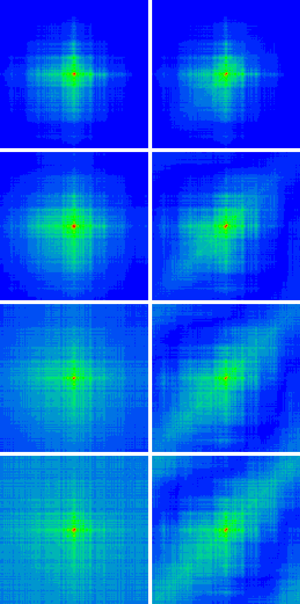
Figure 6: The same as Fig. 5 but for the disorder potential ($W=5$) and all other parameters identical as in Fig. 5.

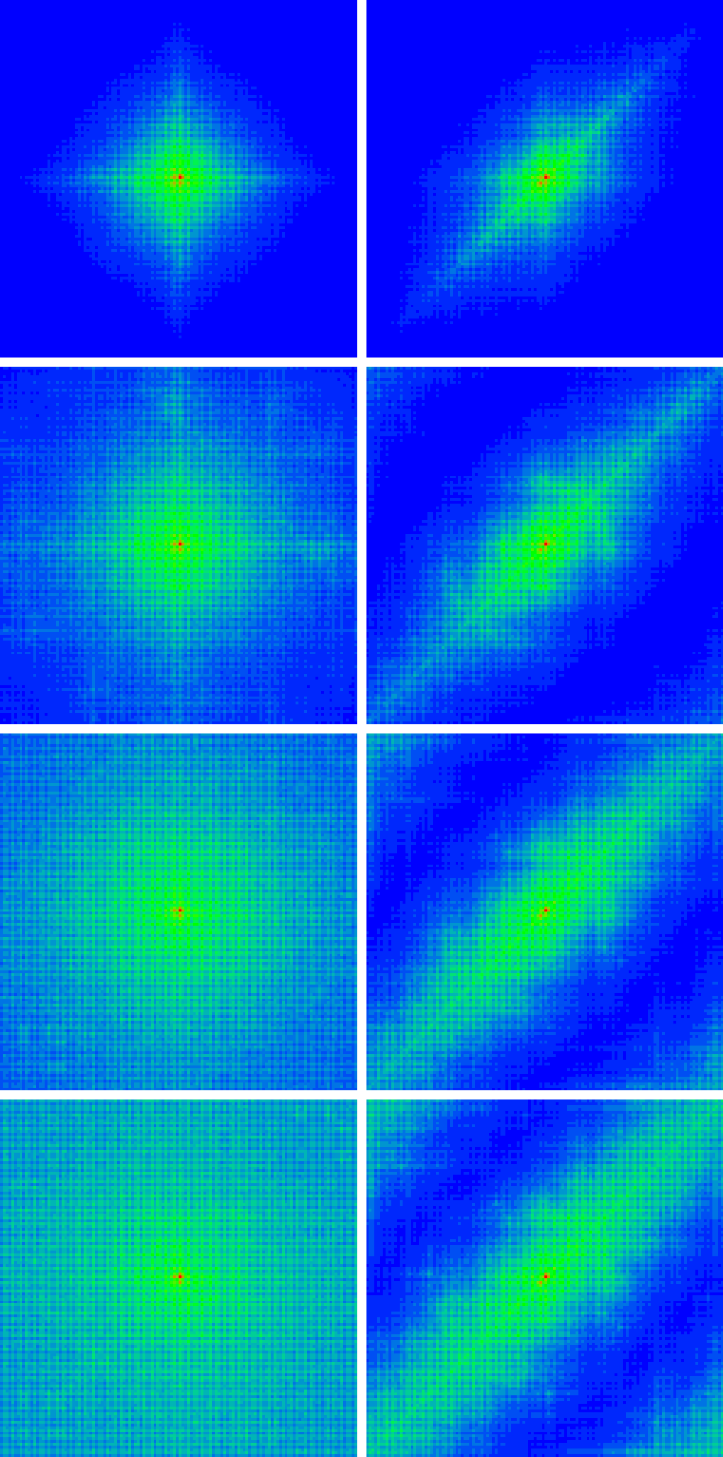
Figure 7: The same as Fig. 5 for the quasiperiodic potential ($\lambda=2.5$) with $U=3.5$, $U_{R}=2$ and all other parameters identical as in Fig. 5.

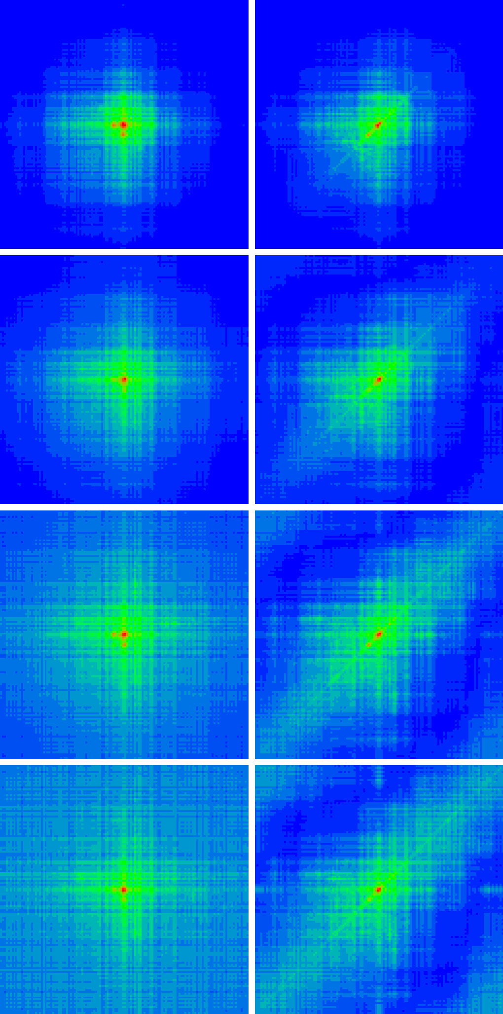
Figure 8: The same as Fig. 5 but for the disorder potential ($W=5$) with $U=3.5$, $U_{R}=2$ and all other parameters identical as in Fig. 5.

The probability distributions for the rectangular geometry are shown in Fig. 9. In this case the width of the cigar is also smaller in the case of the 2D Harper potential as compared to the disorder case. The density at $t=10^{4}$ gives some weak indication on presence of far away probability at large $x_{1}=x_{2}\approx N_{1}$ distances, which would be expected for ballistic FIKS pairs. However, the probability there is very small and also at $t=10^{5}$ both cases show similar probability profiles corresponding to localization of the wave packet.

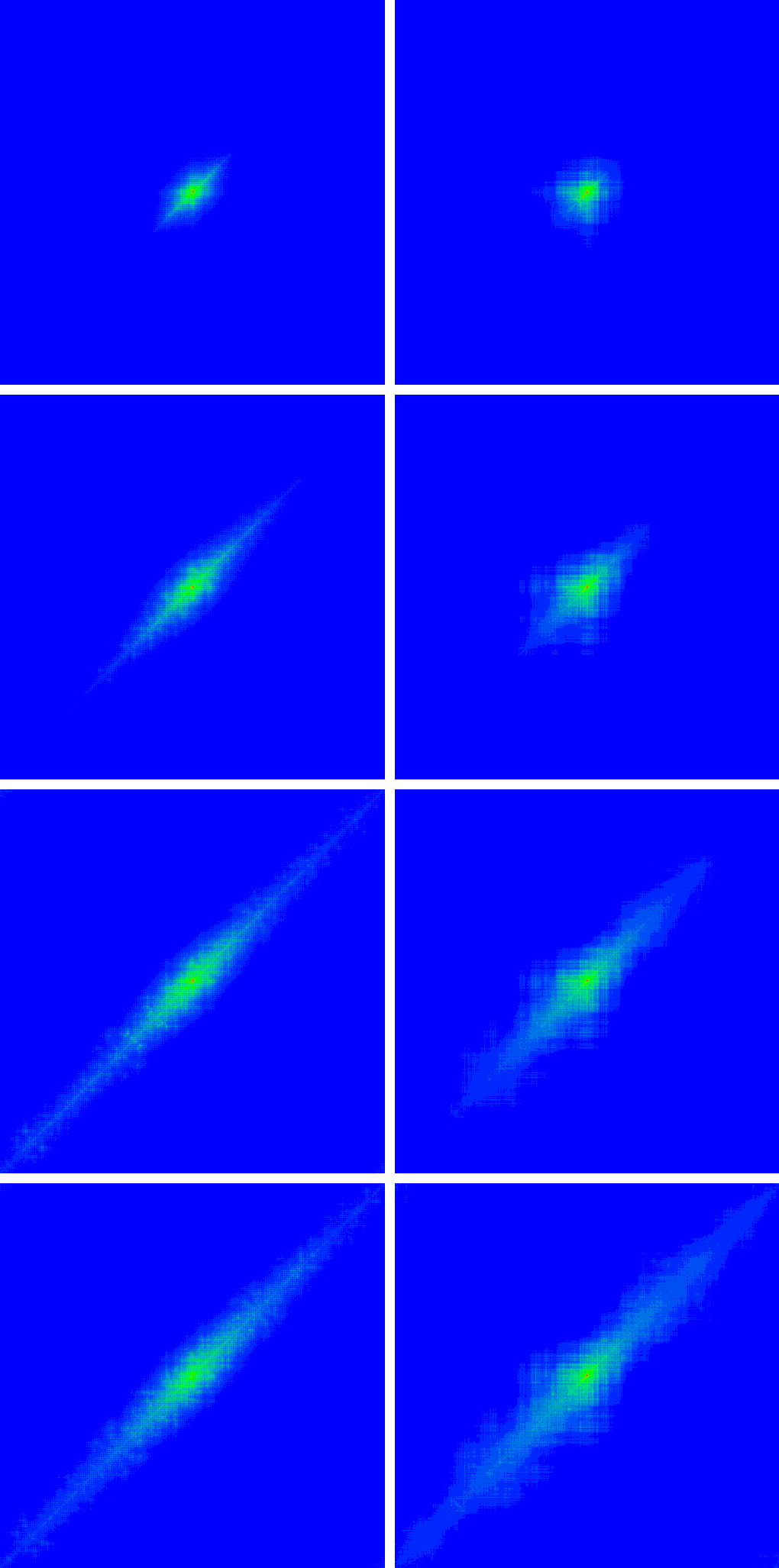
Figure 9: Density plot for the density $\rho_{xx}(x_{1},x_{2})$ with $x_{1}$ for the horizontal axis and $x_{2}$ for the vertical axis. All panels correspond to $U=3.5$, $U_{R}=2$ and the rectangular geometry $N_{1}=512$, $N_{2}=8$. The left column corresponds to the quasiperiodic potential ($\lambda=2.5$) and the right column to the disorder potential ($W=5$). The different rows correspond to the iteration time $t=100$ (first top row), $t=1000$ (second row), $t=10000$ (third row) and $t=100000$ (fourth bottom row).

Finally in Fig. 10 we consider an asymmetric case of the 2D Harper model with $\lambda_{x}=2.5$, $\lambda_{y}=3.5$, $N_{1}=128$ and $N_{2}=48$. Here we have a significantly stronger localization of non-interacting particles in the $y$-direction with $\ell_{y}=1/\log(\lambda_{y}/2)\approx 1.79$. Thus we could expect appearance of 1D ballistic FIKS pairs in such a case. However, this scenario is not confirmed by the data which still give a subdiffusive spreading with the fit exponents $b_{1}=0.563\pm 0.004$ and $b_{2}=0.431\pm 0.016$ for the time range $10\leq t\leq 1000$ and the power law fits $\langle r^{2}\rangle\propto t^{b_{1}}$ and $\xi_{\rm IPR}\propto t^{b_{2}}$. The probability distribution in $x$ becomes rather broad at large times $t=10^{5}$ and it is possible that even larger system sizes are required to firmly state if this subdiffusion continues on longer times. Furthermore the density $\rho_{y}(y)$ does not show a strong localization in the $y$-direction in presence of interaction, despite the very small value of $\ell_{y}$, and there are quite large tails of $\rho_{y}(y)$ for $y$ being close to the transversal boundaries. Therefore the scenario of an effective $1D$-situation in $x$ due to strong $y$-localization does not really happen thus explaining that we have no visible indications for FIKS pairs in such an asymmetric situation.

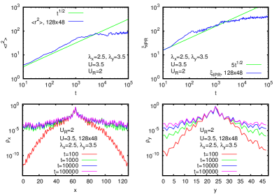
Figure 10: Variance $\langle r^{2}\rangle$ (top left panel) and IPR without center $\xi_{\rm IPR}$ (top right panel) versus iteration time $10\leq t\leq 10^{5}$ in a double logarithmic scale for the asymmetric case of the quasiperiodic potential ($\lambda_{x}=2.5$, $\lambda_{y}=3.5$) with rectangular geometry $N_{1}=128$, $N_{2}=48$ and $U=3.5$, $U_{R}=2$. Both quantities are shown by the blue line and the green line shows for comparison a power law $\sim t^{1/2}$. The bottom left (right) panel shows for the same parameters the density $\rho_{x}(x)$ (or $\rho_{y}(y)$) versus $x$ (or $y$) in a semilogarithmic representation. The color labels correspond to different iteration times: $t=100$ (red curve), $t=1000$ (green curve), $t=10000$ (blue curve), $t=100000$ (pink curve).

4 Discussion

We presented here the study of interaction effects in the 2D Harper model where the two-dimensional quasiperiodic potential is given as the sum of two one-dimensional quasiperiodic potentials for the $x$ and the $y$ direction. Our results show that in this system the interactions induce a subdiffusive spreading over the whole lattice with the spreading exponent being approximately $b\approx 0.5$ for the second moment and IPR. Such a delocalization takes place in the regime when all one-particle eigenstates are exponentially localized. In this 2D TIP Harper model we do not find signs of ballistic FIKS pairs, which are well visible for the 1D TIP Harper case flach ; fiks1d .

It is possible that the physical reason of absence of FIKS pairs in 2D Harper model is related to the fact that for TIP in 2D we have a much more dense spectrum of non-interacting eigenstates [see e.g. Eg.(29) in fiks1d where the indexes $m_{1},m_{2}$ of non-interacting eigenstates of two particles now become vectors in 2D]. Due to this there are practically no well separated energy bands typical for the one-particle 1D Harper model and thus there is little chance to have an effective Aubry-André Hamiltonian with $\lambda_{\rm eff}$ and the interaction induced hopping matrix elements $t_{\rm eff}$ generating a metallic phase with $\lambda_{\rm eff}<2t_{\rm eff}$. Of course, there is still a possibility that we missed some FIKS cases at specific $U$ values but for all studied cases of TIP in the 2D Harper model we find a subdiffusive spreading being qualitatively different from the FIKS effect in the 1D Harper case. For a rectangular geometry with a narrow size band in one direction we even obtain a localization of TIP spreading.

When the quasi-periodic potential is replaced by a disorder potential of the particular form (4) we also find a subdiffusive spreading but with a smaller exponent $b\approx 0.25$ (on available time range and system size). In principle, for TIP in the 2D disorder potential we expect to have localized states for short range interactions imry ; dlsmoriond ; dlscoulomb . However, here we consider a particular correlated disorder (with a potential being a sum of two one-dimensional potentials in $x$ and $y$) and in such a case the one-particle localization length at $W=5$ ($\ell_{1}\approx\xi\approx 5$) is significantly smaller than for the usual 2D disorder potential (see e.g. lagesbls with $\xi\approx 150$). We think that in presence of interactions and sufficient iteration times such correlations of disorder are suppressed and we have a situation similar to the TIP case of the usual 2D Anderson model where at $W=5$ the one-particle localization length $\ell_{1}$ is rather large and thus the TIP localization length $\ell_{2}$, expected to be an exponent of $\ell_{1}$ imry ; dlsmoriond , is also very large ($\ln\ell_{2}\sim l_{1}$) and is not reachable at time scales and system sizes used in our studies. In any case the smaller value of $b\approx 0.25$ for the disorder case, compared to the 2D Harper case with $b\approx 0.5$, indicates that some residual effects of FIKS pairs give a stronger delocalization of TIP for the 2D Harper model.

It is interesting to note that a somewhat similar subdiffusive spreading appears in the 2D Anderson model with a mean field type nonlinearity (see e.g. garcia ). However, there the value of the spreading exponent $b\approx 0.25$ is smaller (the value $b\approx 0.5$ found here is more similar to the 1D Anderson model with nonlinearity studied in danse ; flachdanse ). However, the physical origin of a certain similarity of these nonlinear mean-field models with the TIP case studied here remains unclear since here we have a linear Schrödinger equation while the models of danse ; garcia ; flachdanse are described by classical nonlinear equations (second quantization is absent).

We think that the 2D TIP Harper model provides us new interesting results with subdiffusive spreading induced by interactions. This model rises new challenges for advanced mathematical methods developed for quasiperiodic Schrödinger operators lana2 ; lana3 . It is also accessible to experimental investigations with ultracold atoms in 2D quasiperiodic optical lattices which can be now built experimentally bloch2d . Thus we hope that the TIP problem in 1D and 2D Harper models will attract further detailed theoretical and experimental investigations.

This work was granted access to the HPC resources of CALMIP (Toulouse) under the allocation 2015-P0110.

References

- (1) P.G. Harper, Proc. Phys. Soc. London Sect. A 68, 874 & 879 (1955).
- (2) D.R. Hofstadter, Phys. Rev. B 14, 2239 ̵͑(1976).
- (3) S. Aubry and G. André, Ann. Israel Phys. Soc. 3, 133 (1980).
- (4) J.B. Sokoloff, Phys. Rep. 126, 189 (1985).
- (5) S.Y. Jitomirskaya, Ann. Math. 150, 1159 (1999).
- (6) D.L. Shepelyansky, Phys. Rev. B 54, 14896 (1996).
- (7) A. Barelli, J. Bellissard, Ph. Jacquod, and D.L. Shepelyansky, 77, 4752 (1996).
- (8) G. Dufour, and G. Orso, Phys. Rev. Lett. 109, 155306 (2012).
- (9) D.L. Shepelyansky, Phys. Rev. Lett. 73, 2607 (1994).
- (10) Y. Imry, Europhys. Lett. 30, 405 (1995).
- (11) D. Weinmann, A. Müller–Groeling, J.-L. Pichard, and K. Frahm, Phys. Rev. Lett. 75, 1598 (1995).
- (12) K. Frahm, A. Müller–Groeling, J.-L. Pichard, and D. Weinmann, Europhys. Lett. 31, 169 (1995).
- (13) F. von Oppen, T. Wetting, and J. Müller, Phys. Rev. Lett. 76, 491 (1996).
- (14) F. Borgonovi, and D.L. Shepelyansky, J. de Physique I France 6, 287 (1996).
- (15) D.L. Shepelyansky, in Correlated fermions and transport in mesoscopic systems (Eds. T.Martin, G.Montambaux, J.Tran Thanh Van), Editions Frontieres, Gif-sur-Yvette France, 201 (1996).
- (16) K.M. Frahm, Eur. Phys. J. B, 10, 371 (1999).
- (17) D.L. Shepelyansky, Phys. Rev. B 61, 4588 (2000).
- (18) J. Lages, and D.L. Shepelyansky, Eur. Phys. J. B 21, 129 (2001).
- (19) S. Flach, M. Ivanchenko, and R. Khomeriki, Europhys. Lett. 98, 66002 (2012).
- (20) K.M. Frahm, and D.L. Shepelyansky, http://arxiv.org/abs/1509.02788 (2015).
- (21) G. Roati, C. D‘Errico, L. Fallani, M. Fattori, C. Fort, M. Zaccanti, G. Modugno, M. Modugno, and M. Inguscio, Nature 453, 895 (2008).
- (22) E. Lucioni, B. Deissler, L. Tanzi, G. Roati, M. Zaccanti, M. Modugno, M. Larcher, F. Dalfovo, M. Inguscio, and G. Modugno, Phys. Rev. Lett. 106, 230403 (2011).
- (23) M. Schreiber, S.S. Hodgman, P. Bordia, H. Lüschen, M.H. Fischer, R. Vosk, E. Altman, U. Schneider, and I. Bloch, Science 349, 842 (2015).
- (24) P. Bordia, H.K. Ls̈chen, S.S. Hodgman, M. Schreiber, I. Bloch, and U. Schneider, http://arxiv.org/abs/1509.00478 (2015).
- (25) http://www.quantware.ups-tlse.fr/QWLIB/tipharper2d
- (26) In view of the periodic boundary conditions the condition (or ) is understood to be true also for the case (), i. e. if () is close to one boundary and () to the other boundary.
- (27) A.S. Pikovsky, and D.L. Shepelyansky, Phys. Rev. Lett. 100, 094101 (2008).
- (28) I. Garcia-Mata, and D.L. Shepelyansky, Phys. Rev. E 79, 026205 (2009).
- (29) M. Frigo, A Fast Fourier Transform Compiler, Proc. 1999 ACM SIGPLAN Conf. “Programming Language Design and Implementation (PLDI ’99)”, Atlanta, Georgia, http://www.fftw.org/pldi99.pdf May 1999.
- (30) J. Lages, and D.L. Shepelyansky, Phys. Rev. B 64, 094502 (2001).
- (31) T.V. Lapteva, M.V. Ivanchenko, and S. Flach, J. Phys. A: Math. Theor. 47, 493001 (2014).
- (32) J. Bourgain, and S. Jitomirskaya, Invent. Math. 148, 453 (2002).
- (33) S. Jitomirskaya, and C.A. Marx, http://arxiv.org/abs/1503.05740 (2015).