Intensity-only optical compressive imaging using a multiply scattering material and a double phase retrieval approach

Abstract

In this paper, the problem of compressive imaging is addressed using natural randomization by means of a multiply scattering medium. To utilize the medium in this way, its corresponding transmission matrix must be estimated. For calibration purposes, we use a digital micromirror device (DMD) as a simple, cheap, and high-resolution binary intensity modulator. We propose a phase retrieval algorithm which is well adapted to intensity-only measurements on the camera, and to the input binary intensity patterns, both to estimate the complex transmission matrix as well as image reconstruction. We demonstrate promising experimental results for the proposed double phase retrieval algorithm using the MNIST dataset of handwritten digits as example images.

I Introduction

From the perspective of image processing, the goal of compressed sensing (CS) is to reconstruct a high-resolution image, which is sparse in either the ambient domain or some transform basis, using few incoherent linear projections Romberg (2008). Over the past decade, there has been a tremendous amount of work in the field of CS, including analytical reconstruction guarantees as well as developments of new algorithmic approaches that provide efficient methods of solving the reconstruction task Eldar and Kutyniok (2012); Boche et al. (2015). However, to date there have been only a handful of engineering projects where optical imagers based on CS have actually been built. Indeed, performing these incoherent, usually random, projections is a highly non-trivial task, requiring innovative hardware solutions. Amongst such imagers, one can cite, without any claim of completeness, several single-pixel imaging systems Duarte et al. (2008); Magalhães et al. (2011); Shrekenhamer et al. (2013), a random lens camera Fergus et al. (2006), and an imaging setup based on a rotating diffuser Zhao et al. (2012).

The work presented in this paper is built upon a recently developed optical CS setup Drémeau et al. (2015) that uses a multiply scattering medium to effect the random projection operation. The fundamental difference with this approach and most of the CS systems discussed above is that here the random projections are not designed beforehand and then implemented through sophisticated hardware, as in Gao et al. (2014), but are based on the natural randomization properties of coherent light multiply scattering through a layer of opaque material. Here, the word “multiply” refers to the fact that the thickness of the material slab is many times larger than the mean free path, ensuring that the light beam is fully scattered without any remaining ballistic photons at the output. If $x$ is the incoming wavefield (the object to be imaged at the input plane), the scattering operation is well modeled by a simple linear operator $\mathbf{H}$, called the transmission matrix. If $y$ is the output wavefield discretized by receptor pixels, then, in the ideal noiseless case,

$$y=\mathbf{H}x.$$ (1)

It has been shown that the transmission matrix of a scattering material is statistically identical to an i.i.d. random matrix with a complex Gaussian distribution Popoff et al. (2010). The benefits of using such a system for CS imaging are that one does not have to rely on complex engineering solutions to provide the (pseudo-) randomization, and also that, in theory, only one shot is necessary to obtain any desired number of output features; as opposed to the single-pixel camera which intrinsically requires sequential measurements.

There exists, however, an obvious price to pay: the necessity of a precise calibration step. Indeed, to be able to use this system as an imaging device, i.e. to estimate $x$ given measurements $y$, one must have accurate knowledge of the matrix $\mathbf{H}$. This can be accomplished by sending a series of known images, measuring the corresponding outputs, and performing a least-squares estimate of $\mathbf{H}$. The calibration step is conducted by shaping the input wavefront with a Spatial Light Modulator (SLM), which is only used for calibration and display, and is not part of the direct imaging system.

In this paper, we circumvent one major limitation of the previous proof-of-concept system Liutkus et al. (2014). Since optical sensors (here, a CCD camera) only measure the field intensity $|y|^{2}$, in Liutkus et al. (2014) the input image is phase-modulated using a phase-only SLM, with relative phases $0$, $\pi/4$, $\pi/2$, and $3\pi/4$. Combining the corresponding four output intensity images, one can easily recover the complex field $y$ using a method known as “phase-stepping holography”. Furthermore, such phase-only modulated images have a constant intensity. To obtain an image that is sparse in the spatial domain, one has to make the difference between 2 complex phase-only images which only differs by a sparse number of pixels. Therefore, in order to get the complex measurements corresponding to a single sparse image, 8 intensity measurements are required. This significantly slows down both the calibration and the measurement process. Furthermore, a sufficiently fast continuous-phase SLM is a very expensive device, with limited pixel counts. For example, the SLM used in Liutkus et al. (2014) could only display $32\times 32$ images.

Here, we investigate the alternative use of a digital micro-mirror device (DMD) as an SLM, as shown in Fig. 1. This has many advantages: DMDs are cheap, fast, and have high pixel counts. However, the main drawback of these binary intensity modulators is that, without additional hardware, one can no longer use phase-stepping to measure the complex output field. Instead of using hardware to measure amplitude and phase, we resort to “phase retrieval” in order to estimate the missing phases from intensity-only measurements $|y|^{2}$. It should be noted that, in this framework, phase retrieval must be applied twice successively; first, for the calibration, and second, for the imaging itself. The success of the second step crucially depends on the first one, as every error in estimating H results in multiplicative noise (also called model error) in the imaging step. It should also be noted that the signal-to-noise ratio is relatively poor, thus we favor Bayesian phase retrieval techniques where noise may be explicitly modeled.

The main contributions of this paper are as follows:

• A new Bayesian phase retrieval algorithm known as phase retrieval Swept AMP (prSAMP). prSAMP originates from prGAMP Schniter and Rangan (2015) and SwAMP Manoel et al. (2014) and is designed to work with noisy ill-conditioned transmission matrices.

• The experimental demonstration that prSAMP is efficient both for calibration of the non-sparse measurement matrix H using binary inputs, and for intensity-only CS imaging of sparse inputs.

Although our previous studies Liutkus et al. (2014) demonstrate a proof-of concept that CS-based imaging can be made with multiply scattering materials, we believe that this one-shot imager represents a very significant step toward real-life applications of these techniques.

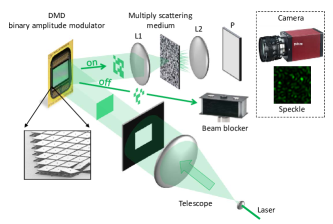
Figure 1: Experimental setup of the imager, from Drémeau et al. (2015). A monochromatic laser at 532 nm is expanded by a telescope and illuminates an SLM, here, a Texas Instruments DLP9500 DMD with 1920$\times$1080 pixels. The light beam carrying the image is then focused on a random medium by means of a microscope lens. Here, the medium is a thick (several tens of microns) opaque layer of Zinc Oxide nanoparticles deposited on a glass slide. The transmitted light is collected on the far side by a second lens, passes through a polarizer, and is detected by an AVT PIKE F-100 monochrome CCD camera. Note that the DMD is only for calibration and display and is not part of the imager itself.

II Theoretical modeling

Starting from the idealized model of Eq. (1), we formalize the calibration procedure as in Drémeau et al. (2015). Given $P$ known binary input images of size $N=n_{1}\times n_{2}$, $\textbf{X}\in\{0,1\}^{P\times N}$, and their corresponding intensity measurements on $M$ output pixels, $\textbf{Y}\in\mathbb{R}_{+}^{M\times P}$, $M$ independent phase retrieval problems are solved during the calibration step to estimate the transmission matrix $\textbf{H}\in\mathbb{C}^{M\times N}$. Each calibration problems is formulated as

$$\textbf{y}_{\rm m}^{T}=|\textbf{X}\textbf{h}_{\rm m}^{T}|,$$ (2)

where $(\cdot)_{m}$ indicates the $m$-th row of corresponding matrix and $(\cdot)^{T}$ is the transpose operator. The process of recovering a signal from only the magnitude of its projections is the goal of phase retrieval Candes et al. (2015); Iwen et al. (2015); Schniter and Rangan (2015). Apart from additional noise in the measurements, what makes solving Eq. (2) challenging is using binary input patterns, since most well-known phase retrieval methods work well with complex-valued measurement matrices. We have fixed this issue by mixing the ideas of Swept Approximate Message Passing (SwAMP) Manoel et al. (2014), which demonstrates good convergence properties over ill-conditioned noisy matrices, with the phase retrieval method prGAMP Schniter and Rangan (2015). The new prSAMP algorithm is explained in the next section.

After calibration, the setup can be used as a generalized CS imager with non-linear (intensity) measurements. In this reconstruction phase, the noiseless model becomes $\textbf{y}=|\textbf{H}\textbf{x}|$. We use the same prSAMP method, with different priors, to solve both the calibration and reconstruction tasks.

III prSAMP algorithm

In the context of CS, AMP is an iterative algorithm for the reconstruction of a sparse signal from a set of under-determined linear noisy measurements $\textbf{y}=\textbf{H}\textbf{x}+\textbf{w}$, where $\textbf{w}\sim\mathcal{N}(0,\sigma^{2})$ Maleki (2010). Although this method originates from loopy belief propagation, it does not suffer from the same computational complexity. AMP has been shown to be effective with a minimal number of measurements while being efficient in terms of computational complexity. Using a Bayesian approach, the main loop of AMP consists of iteratively updating the estimated mean $\textbf{x}_{\rm a}$ and variance $\textbf{x}_{\rm v}$ of the unknown signal until convergence,

$$\textbf{v}^{t} =|\textbf{H}|^{2}\textbf{x}_{\rm v}^{t-1},$$ (3)

$$\bm{\omega}^{t} =\textbf{H}\textbf{x}_{\rm a}^{t-1}-(\textbf{y}-\bm{\omega}^{t-1})\circ\textbf{v}^{t}\circ(\textbf{v}^{t-1}+\sigma^{2})^{-1},$$ (4)

$$\textbf{s}^{t} =[|\textbf{H}^{*}|^{2}(\textbf{v}^{t}+\sigma^{2})^{-1}]^{-1},$$ (5)

$$\textbf{r}^{t} =\textbf{x}_{\rm a}^{t}+\textbf{s}^{t}\circ\textbf{H}^{*}[(\textbf{y}-\bm{\omega}^{t})\circ(\textbf{v}^{t}+\sigma^{2})^{-1}],$$ (6)

$$[\textbf{x}_{\rm a}^{t} ,\;\textbf{x}_{\rm v}^{t}]=\textit{p}_{\rm in}(\textbf{r}^{t},\textbf{s}^{t}),$$ (7)

where $\circ$ is the element-wise Hadamard product, $(\cdot)^{-1}$ is understood to be an element-wise reciprocal, $(\cdot)^{t}$ is a time index, $(\cdot)^{*}$ is the conjugate-transpose, and $\textit{p}_{\rm in}$ is a function based on the desired signal prior which returns both the mean and variance estimate of the unknown signal. We refer the reader to Krzakala et al. (2011) for a detailed description of Bayesian AMP. The calibration and reconstruction phases employ Gaussian and binary priors, respectively Krzakala et al. (2012); Barbier et al. (2012). From Popoff et al. (2010), we know that the transmission matrices of scattering mediums appear to be i.i.d. random matrices. Therefore, a Gaussian prior for the calibration phase is a reasonable choice. For the reconstruction phase, two binary priors have been investigated based on global (per-image) and local (per-pixel) sparsity, the details of which are explained in the next section.

Generalized AMP (GAMP) Schniter and Rangan (2015) is an extension of AMP for arbitrary output channels, i.e. $\textbf{y}=q(\textbf{H}\textbf{x}+\textbf{w})$. This adds an output function, $\textit{p}_{\rm out}$, which is dependent on the stochastic description of $q(\cdot)$. In Eqs. (4)-(6), the terms $(\textbf{y}-\bm{\omega}^{t})\circ(\textbf{v}^{t-1}+\sigma^{2})^{-1}$ and $-(\textbf{v}^{t}+\sigma^{2})^{-1}$ indicate $\textit{p}_{\rm out}$ and $\textit{p}^{\prime}_{\rm out}$, respectively, for a Gaussian output channel. One can easily modify these two terms in order to extend the framework to other channels. Following Schniter and Rangan (2015), for the phase retrieval problem we have

$$\textit{p}_{\rm out} =\bm{\omega}\circ(\textbf{v}+\sigma^{2})^{-1}\circ(r_{0}\textbf{y}\circ|\bm{\omega}|^{-1}-1),$$ (8)

$$\textit{p}^{\prime}_{\rm out} =(\textbf{v}+\sigma^{2})^{-1}\circ\left[\frac{(1-r_{0}^{2})\textbf{y}^{2}}{(\textbf{v}+\sigma^{2})}+\frac{\sigma^{2}}{\textbf{v}}\right]-\textbf{v}^{-1},$$ (9)

where $r_{0}=\frac{I_{1}(\phi)}{I_{0}(\phi)}$, $I_{0}$ and $I_{1}$ are $0^{\rm th}$ and $1^{\rm st}$ order modified Bessel functions of first kind, respectively, and $\bm{\phi}=2\textbf{y}\circ|\bm{\omega}|\circ(\textbf{v}+\sigma^{2})^{-1}$.

The convergence of both AMP and GAMP has been proved for zero-mean i.i.d. measurement matrices Bayati and Montanari (2011), however, they do not necessarily converge for generic matrices Caltagirone et al. (2014). There have been some attempts to prevent divergence of AMP-based methods Vila et al. (2015); Manoel et al. (2014); Çakmak et al. (2014). In Manoel et al. (2014), the authors show that a simple change in the main AMP loop may stabilize AMP significantly. They propose a sequential, or swept, random update of the AMP messages $\textbf{s}^{t}$, $\textbf{r}^{t}$, $\textbf{x}_{\rm a}^{t}$ and $\textbf{x}_{\rm v}^{t}$, instead of their standard parallel calculation. By combining the swept update ordering and the phase retrieval output channel (8)-(9) in the AMP iteration (3)-(7), we create a phase retrieval version of SwAMP, denoted as prSAMP, which we describe in Algorithm 1.

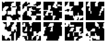
Figure 2: Examples of structured patterns used for calibration.

IV Experimental Results

To investigate the performance of the proposed imaging system, two binary datasets are constructed from the spatially-sparse MNIST handwritten dataset. The first, $D_{1}$, consists of cropped digit images at a resolution of $20\times 20$ pixels ($N=400$). The second, $D_{2}$, is constructed by rescaling the MNIST dataset to $32\times 32$ pixels ($N=1024$). Both $D_{1}$ and $D_{2}$ retain the original MNIST training/testing partition.

For the calibration step, training set $D_{1}$ is modified by randomly exchanging $5\times 5$ blocks of pixels between digit images. Fig. 2 shows a few samples of these structured patterns. This structured randomization is done to reduce the effect of correlation between the DMD pixels. Additionally, to avoid the possibility of completely zero, or very sparse, lines in X, see Eq. (2), we introduce a fixed number of unstructured i.i.d. Bernoulli random binary patterns to the calibration training set.

The transmission matrix is then estimated from $P=\alpha N$ calibration images, of which the first $N$ are Bernoulli random patterns, for the oversampling ratio $\alpha\geq 1$. At the receptor, $M$ samples are randomly selected from a $100\times 100$ region of the output image. Fig. 3 (left) shows the performance of the proposed calibration method for varying values of $\alpha$. In lieu of ground-truth comparisons for transmission matrix estimation, we assess the calibration performance in terms of “dependence,” the normalized cross-correlation without mean removal, $\left\langle\frac{\textbf{y}}{\left\lVert\textbf{y}\right\rVert},\frac{|\textbf{H}\textbf{x}|}{\left\lVert\textbf{H}\textbf{x}\right\rVert}\right\rangle$, between observed samples and the predicted output of known input patterns using the estimated transmission matrix. We measure dependence over 400 digits from the testing set of $D_{1}$. We compare the level of achieved dependence between prSAMP and prVBEM Drémeau et al. (2015), a mean-field variational Bayes phase retrieval technique we previously employed for the task of transmission matrix calibration in the context of light focusing.

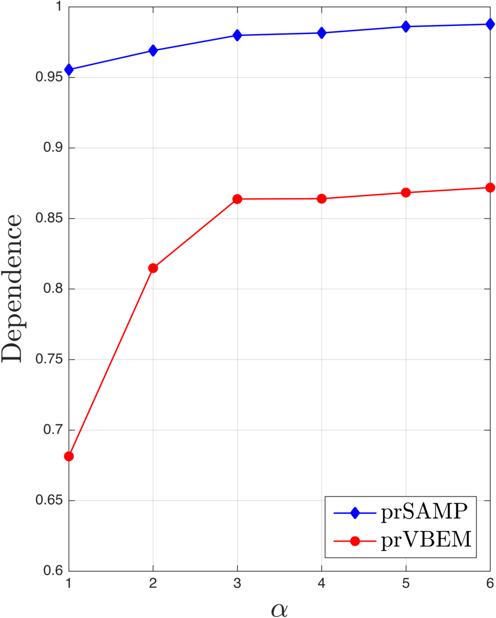
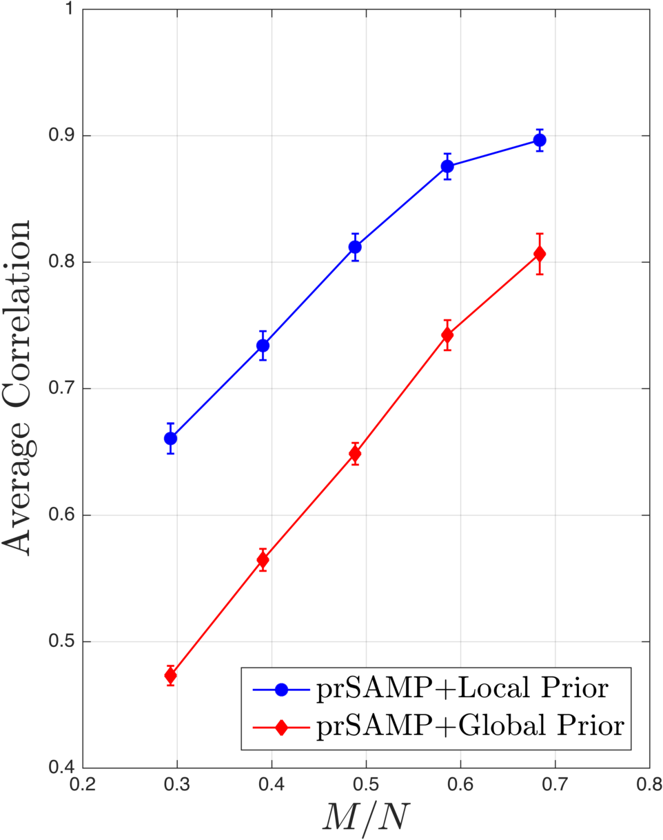
Figure 3: Left: Calibration performance of both prSAMP and prVBEM for varying numbers of calibration patterns $P=\alpha N$ which are generated from the $D_{1}$ dataset. Right: Reconstruction performance over 50 digits of $D_{2}$ ($N=1024$) using prSAMP with both global and local binary priors for $M=\left\{300,400,500,600,700\right\}$ output samples.

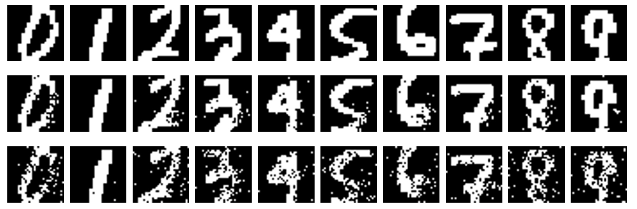
Figure 4: Visual performance of prSAMP reconstruction for 32$\times$32 images at $M=700$. Top row: Original images. Middle row: prSAMP with local prior. Bottom row: prSAMP with global prior.

After calibration, the direct imaging phase can start. As described in Section III, the calibration and reconstruction steps are performed using the same prSAMP algorithm with different input priors. During calibration, we assume a complex Gaussian prior since the transmission matrix is modeled as i.i.d. random. However, for reconstruction, a binary prior is required,

$$x_{{\rm a}i}^{t} =\frac{\rho_{i}}{z_{i}}\textit{e}^{\frac{-|1-r_{i}^{t}|^{2}}{2s_{i}^{t}}},\quad x_{{\rm v}i}^{t}=x_{{\rm a}i}^{t}-(x_{{\rm a}i}^{t})^{2},$$ (10)

where $z_{i}=(1-\rho_{i})\textit{e}^{\frac{-|r_{i}^{t}|^{2}}{2s_{i}^{t}}}+\rho_{i}\textit{e}^{\frac{-|1-r_{i}^{t}|^{2}}{2s_{i}^{t}}}$, and $\rho_{i}$ indicates the probability of pixel $i$ to be non-zero. We use two strategies to set this parameter. The first is a global approach which sets all $\rho_{i}$ uniformly to the input image sparsity level which we assume is known up to some tolerance. In the second local approach, we empirically calculate the per-pixel non-zero probability using the calibration training set, which is a fast off-line process. As the prior calculation must be repeated at each pixel for each sweep of the prSAMP algorithm, we select the simplest possible prior for the sake of computational efficiency. The interested reader may refer to Tramel et al. (2016) for a more sophisticated method of using learned priors for reconstruction tasks.

We next use the $D_{2}$ dataset to study the effectiveness of prSAMP post-calibration reconstruction. We first perform the calibration step to estimate $M=N$ rows of the transmission matrix using $\alpha=5$, yielding an average calibration correlation of 97% over 1024 test digits. For reconstruction, we randomly choose 50 images from the test set, with five images for each digit. The correlation of prSAMP reconstructions to the true inputs, using global and local binary priors, are compared in Fig. 3 (right) as a function of the measurement rate $M/N$. Leveraging the extra information in the local prior provides an average 14.87% increase in reconstruction performance over the global prior. To visually assess the quality of recovered images, Fig. 4 provides one instance from each digit recovered at $M=700$, with reconstructions using the local and the global priors. As expected, the local prior provides better subjective quality with fewer spurious isolated pixels.

V Conclusion

In this study, a phase retrieval compressive imager has been proposed and experimentally evaluated using a simple optical setup. The imager has the potential of providing high resolution images in one shot. We solve the challenging problem of estimating a complex transmission matrix using binary patterns and we solve the phase retrieval problem via swept AMP. Finally, we show that we can estimate the transmission matrix accurately, allowing it to be used for compressive imaging. Further studies are necessary to provide faster calibration methods.

VI Acknowledgment

The authors would like to thank Christophe Schülke for his enlightening comments. This research has received funding from the European Research Council under the EU’s 7th Framework Programme (FP/2007- 2013/ERC Grant Agreement 307087-SPARCS and 278025- COMEDIA) ; and from LABEX WIFI under references ANR-10-LABX-24 and ANR-10-IDEX-0001-02-PSL^⋆.

References

- Romberg (2008) J. Romberg, IEEE Signal Proc. Mag. 25, 14 (2008).
- Eldar and Kutyniok (2012) Y. Eldar and G. Kutyniok, Compressed Sensing: Theory and Applications (Cambridge Uni. Press, 2012).
- Boche et al. (2015) H. Boche, R. Calderbank, G. Kutyniok, and J. Vybíral, Compressed Sensing and its Applications (Springer, 2015).
- Duarte et al. (2008) M. Duarte, M. Davenport, D. Takhar, J. Laska, T. Sun, K. Kelly, and R. Baraniuk, IEEE Signal Proc. Mag. 25, 83 (2008).
- Magalhães et al. (2011) F. Magalhães, F. Araújo, M. Correia, M. Abolbashari, and F. Farahi, Appl. Opt. 50, 405 (2011).
- Shrekenhamer et al. (2013) D. Shrekenhamer, C. Watts, and W. Padilla, Opt. Express 21, 12507 (2013).
- Fergus et al. (2006) R. Fergus, A. Torralba, and W. Freeman, MIT CSAIL Tech. Report (2006).
- Zhao et al. (2012) C. Zhao, W. Gong, M. Chen, E. Li, H. Wang, W. Xu, and S. Han, Appl. Phys. Lett. 101, 141123 (2012).
- Drémeau et al. (2015) A. Drémeau, A. Liutkus, D. Martina, O. Katz, C. Schülke, F. Krzakala, S. Gigan, and L. Daudet, Opt. Express 23, 11898 (2015).
- Gao et al. (2014) L. Gao, J. Liang, C. Li, and L. Wang, Nature 516 (2014).
- Popoff et al. (2010) S. Popoff, G. Lerosey, R. Carminati, M. Fink, A. Boccara, and S. Gigan, Phys. Rev. Lett 104, 100601 (2010).
- Liutkus et al. (2014) A. Liutkus, D. Martina, S. Popoff, G. Chardon, O. Katz, G. Lerosey, S. Gigan, L. Daudet, and I. Carron, Sci. Rep. 4 (2014).
- Schniter and Rangan (2015) P. Schniter and S. Rangan, IEEE Trans. on Signal Proc. 63, 1043 (2015).
- Manoel et al. (2014) A. Manoel, F. Krzakala, E. Tramel, and L. Zdeborová, in Int. Conf. on Machine Learning (2014).
- Candes et al. (2015) E. Candes, Y. Eldar, T. Strohmer, and V. Voroninski, SIAM Rev. 57, 225 (2015).
- Iwen et al. (2015) M. Iwen, A. Viswanathan, and Y. Wang, arXiv preprint:1501.02377 (2015).
- Maleki (2010) A. Maleki, Approximate Message Passing Algorithms for Compressed Sensing, Ph.D. thesis, Stanford Uni. (2010).
- Krzakala et al. (2011) F. Krzakala, M. Mézard, F. Sausset, Y. Sun, and L. Zdeborová, Phys. Rev. X 2 (2011).
- Krzakala et al. (2012) F. Krzakala, M. Mézard, F. Sausset, Y. Sun, and L. Zdeborová, J. Stat. Mech.: Theory & Exp. 2012, P08009 (2012).
- Barbier et al. (2012) J. Barbier, F. Krzakala, M. Mézard, and L. Zdeborová, in IEEE Allerton Conf. on Comm., Control, & Computing (2012) pp. 800–807.
- Bayati and Montanari (2011) M. Bayati and A. Montanari, IEEE Trans. on Info. Theory 57, 764 (2011).
- Caltagirone et al. (2014) F. Caltagirone, L. Zdeborová, and F. Krzakala, in IEEE Int. Symp. on Info. Theory (2014) pp. 1812–1816.
- Vila et al. (2015) J. Vila, P. Schniter, S. Rangan, F. Krzakala, and L. Zdeborová, in IEEE Int. Conf. on Acoustics, Speech, & Signal Proc. (2015) pp. 2021–2025.
- Çakmak et al. (2014) B. Çakmak, O. Winther, and B. Fleury, in IEEE Info. Theory Work. (2014) pp. 192–196.
- Tramel et al. (2016) E. Tramel, A. Drémeau, and F. Krzakala, J. Stat. Mech.: Theory & Exp. (2016), to appear.