Evolution of initially contracting Bianchi Class A models in the presence of an ultra-stiff anisotropic pressure fluid

Abstract

We study the behaviour of Bianchi class A universes containing an ultra-stiff isotropic ghost field and a fluid with anisotropic pressures which is also ultra-stiff on the average. This allows us to investigate whether cyclic universe scenarios, like the ekpyrotic model, do indeed lead to isotropisation on approach to a singularity (or bounce) in the presence of dominant ultra-stiff pressure anisotropies. We specialise to consider the closed Bianchi type IX universe and show that when the anisotropic pressures are stiffer on average than any isotropic ultra-stiff fluid then, if they dominate on approach to the singularity, it will be anisotropic. We include an isotropic ultra-stiff ghost fluid with negative energy density in order to create a cosmological bounce at finite volume in the absence of the anisotropic fluid. When the dominant anisotropic fluid is present it leads to an anisotropic cosmological singularity rather than an isotropic bounce. The inclusion of anisotropic stresses generated by collisionless particles in an anisotropically expanding universe is therefore essential for a full analysis of the consequences of a cosmological bounce or singularity in cyclic universes.

1 Introduction

The standard model of cosmology has been subjected to detailed scrutiny by recent WMAP and Planck mission data. It predicts an almost isotropic, homogeneous and flat expanding universe, an approximately scale-invariant inhomogeneity spectrum with some level of statistical non-gaussianity, and observational parameters linked by an underlying inflationary model for its very early history. This inflationary model requires an early period of accelerated expansion to account for the horizon and flatness problems, and to generate density perturbations that seed the formation of galaxies. Despite the success of the inflationary paradigm, it has little to say about the initial state of the universe and if, or how, a big bang singularity prior to inflation might be avoided or mitigated.

Problems such as these have prompted the search for alternatives to inflation or natural initial conditions that lead to inflation. The philosophy behind these searches is that although inflation is a very successful theory, it is important to search for alternative theories which can provide the similar predictions as inflation, yet which might be distinguished by some decisive observations. One of the oldest alternatives is that of a non-singular bounce.

The existence of a non-singular bounce which facilitates the transition from an initially contracting universe to an expanding one was first hypothesized in general-relativistic cosmology by Tolman and Lemaître [1, 2] and was updated to include more general aspects of general relativistic cosmology and the presence of a cosmological constant by Barrow and Dabrowski [3], [4]. It also regained popularity in the context of pre-big-bang scenarios [5], which although not successful, led to developments in theories which could possess a non-singular bounce. These are usually produced by the addition to standard cosmology of an effective field which violates the null energy condition (NEC). For example, cosmologies with ghost condensates or Galilean genesis take this approach [6]. This has also been used effectively in quantum editions of cosmology, especially in loop quantum cosmology [7], in theories involving canonical quantization of gravity [8, 9], or classical theories with varying constants [10], [11] and ghost fields [12].

One of the first questions to ask when considering alternatives (or additions) to standard inflation is whether it solves the problems that inflation claims to solve. For example, one can ask whether the present-day isotropy and homogeneity of the universe can be achieved through a cosmology which underwent contraction and bounce at some time (or times) in the past. It has been claimed that models implementing a phase of ekpyrosis, or a phase of scalar field-driven fast contraction can indeed solve this problem [13], [14], [15]. In effect, this model claims to solve the anisotropy problem by introducing a scalar field with negative potential energy, which behaves as an ideal fluid with ultra-stiff equation of state $p\gg\rho$. Its isotropic density therefore grows faster than the anisotropies in a contracting universe because the latter diverge no faster than an effective $p=\rho$ fluid. However, this simple analysis assumes that the matter pressure distribution is isotropic. A full analysis needs to include the effects of matter sources with anisotropic pressure distributions on approach to the singularity. Since the isotropic pressure is assumed to exceed the energy density, it should be permitted for the average pressure to exceed the energy density of the anisotropic fluid as well. The need to include anisotropic pressures on approach to the singularity is important because interactions all become collisionless at a higher temperature in the case of anisotropic expansion, than in the isotropic case. Their interaction rates can be written as $\Gamma=\sigma nv\sim g\alpha^{2}T,$, where $\sigma$ is the interaction cross section, $n$ is the number density of particles, $v$ is the average velocity of the particles, $\alpha$ is the generalised structure constant associated with any interaction mediated by some gauge boson, $T$ is the temperature of the universe and $g$ is the effective number of relativistic degrees of freedom of particles at the temperature $T$ . This interaction rate will be slower than the cosmological expansion rate, $H\simeq g^{1/2}T^{2}m_{p}^{-1}$, whenever $T>g^{1/2}\alpha^{2}m_{p}\sim 10^{16}GeV$ in simple unified models. In the preceding line $m_{p}$ is the Planck mass. If the expansion is anisotropic down to a temperature $T_{F}$, the expansion rate is faster, by a factor of $T/T_{F}$. As $\Gamma/H=(T_{F}/T^{2})g^{1/2}\alpha^{2}m_{p}$ at $T>T_{F}$, collisional equilibrium is even harder to maintain when $T>T_{F}$. Graviton production near $T=m_{p}$ also produces a population of collisionless particles whose free streaming will produce significant anisotropic pressures if the expansion dynamics are anisotropic [16], [17].

In this paper, we investigate the effects of anisotropic pressures in the Bianchi Class A homogeneous, anisotropic cosmologies, generalising the study of these effects in the simple Bianchi type I cosmological model by Barrow and Yamamoto [18]. We carry out a generalized phase-plane analysis for all the cosmologies of this type but then focus on the closed Bianchi type IX cosmologies and carry out numerical calculations to study their behaviour near any initial singularity or expansion minimum when this kind of anisotropic matter content is present in addition to an ultra-stiff isotropic fluid. We will show that in these most general homogeneous and anisotropic cosmologies it is essential to include the effects of anisotropic pressures as well as shear anisotropy. When the anisotropic pressures are stiffer on average than the isotropic pressures then they determine the nature of any singularity (or bounce) and it will be dominated by anisotropy, contrary to the situation expected in the standard ekpyrotic picture which ignores anisotropic pressures.

This paper is organised as follows. We begin by presenting the generalised Einstein field equations in an expansion-normalised dynamical system for the non-tilted Bianchi Class A models containing isotropic ultra-stiff ($p>\rho$) matter content as well as a second ultra-stiff matter source with positive density and anisotropic pressures. We first perform a stability analysis on this system for an initially contracting universe to see if a phase of ekpyrosis is really successful in suppressing the anisotropies in the presence of a dominant anisotropic pressure fluid. We also seek solutions to these equations in the limit of small anisotropy and give a new Bianchi I exact solution. In the next section, we study explicitly the evolution of a contracting, anisotropic but spatially homogeneous universe near the initial singularity in the presence of the matter content prescribed, then specializing to the Bianchi type IX universe. We then show the results of our numerical calculations in this universe and compare our results to the results of the stability analysis of the previous section. In the last section we draw our conclusions.

2 Ekpyrotic models

In this section, we first review the simplest ekpyrotic models and the way they suppress the dominant growth of anisotropies in a contracting universe as it approaches the singularity. The ekpyrotic models [14, 19] were originally based on a $5$-dimensional braneworld scenario, where the fifth dimension ends at two boundary branes, one of them being our universe. The branes could interact with each other only gravitationally and are attracted by inter-brane tension during the phase of ekpyrosis. Thus, the universe underwent a phase of slow contraction before the collision and re-expansion of the branes, an event which was identified with the hot big bang. The branes were not completely uniform. Quantum fluctuations cause their collision to occur at different times in different places. Thus some parts of the universe end up hotter than others, giving rise to density and temperature fluctuations. This model has been criticized due to fine tuning problems [20], problems regarding the contracting phase seeming to end in a singularity [21], and also because of its failure to produce a scale-invariant spectrum of density fluctuations [22]. To circumvent such problems, some modifications were proposed in terms of a cyclic model [23, 24, 25], with alternating phases of contraction (when the branes approach each other) and expansion (when the branes are pulled apart and the universe enters a phase of dark-energy domination) occurring simultaneously in a cycle. New versions still attract debate about fundamental issues [41, 40]. The turnaround from contraction to expansion was hypothesized to occur in the form of a non-singular bounce facilitated by a ghost condensation mechanism [15]. Furthermore, it was seen that a scale-invariant density fluctuation power-spectrum could be generated in the new ekpyrotic scenario if one considered two-field ekpyrosis [15]. These possibilities have sustained interest in the ekpyrotic scenario as an alternative to inflation for the origin of structure in the universe. If primordial gravitational waves were reliably detected [26] then their amplitude could provide a decisive test between the two alternatives (and others [27]).

2.1 Effects on expansion anisotropy

As mentioned above, this model also claims to solve the problem of growing shear by incorporating the ekpyrotic phase [13, 15]. This ekpyrotic phase has also been used in other cosmological bouncing models as a way to deal with the problem of growing anisotropies in a contracting universe [28], and so merits closer investigation. For simplicity, we shall focus on the single-field ekpyrotic model and first describe the effects of ekpyrosis in a Bianchi I universe with the ekpyrotic field and an ultra-stiff energy source with anisotropic pressure. The ekpyrotic field is a scalar field, $\phi$ rolling down rapidly on a steep negative potential. This can be viewed as driving the contraction of the universe. To see how it might suppress the anisotropies, we write down its effective equation of state [13].

$$p=(\gamma-1)\rho,\;\;\;\;\;\;\;\;\;\;\;\gamma\gg 2.$$ (1)

The anisotropy energy density scales as $1/l^{6}$, and behaves like a source with $\gamma=2$, $l$ being the time dependent mean scale factor of the universe. Thus, the ekpyrotic phase simply introduces a source which scales with scale factor faster than the energy density in the anisotropy because $\gamma>2$, see [29]. As the universe contracts, this term dominates over the anisotropy in the Friedmann equation, apparently solving the problem of isotropising the universe before it enters the hot big bang phase – or at least preventing the new expanding phase beginning with highly anisotropic dynamics. This should also result in significant dissipation and particle production which would reduce anisotropy and generate entropy [16], [30]. We ignore these complicated effects here.

The simplest form of an anisotropic but spatially homogeneous universe is the Bianchi I (or Kasner) universe [31], [32]. The metric is

$$ds^{2}=-dt^{2}+a^{2}(t)dx^{2}+b^{2}(t)dy^{2}+c^{2}(t)dz^{2},$$ (2)

The Einstein equations for this model gives [33]

$$3H^{2}=\sigma^{2}+\rho_{matter},$$ (3)

$$\dot{\sigma}_{\alpha\beta}+3H\sigma_{\alpha\beta}=\mu\mathcal{P}_{\alpha\beta}$$ (4)

where $\sigma_{\alpha\beta}$ is the shear tensor which follows the relation

$$\sigma^{2}=\frac{1}{2}\sigma^{\alpha\beta}\sigma_{\alpha\beta}$$ (5)

and $\mu$ is the anisotropic pressure fluid density and the definition of $\mathcal{P}_{\alpha\beta}$ is shown in Equation (11). Also $\rho_{matter}$ refers to the total energy density of the matter components of the system, i.e., the matter with isotropic pressures as well as the matter with anisotropic pressure. If we have only a fluid with isotropic pressure, then the right-hand side of Equation (4) vanishes and we can write the shear energy density, $\sigma^{2}$ in the Friedmann constraint, Equation (3) as $\Sigma^{2}/l^{6}$, where $\Sigma^{2}$ is constant. Hence, an ekpyrotic field with equation of state, $p_{\phi}\gg\rho_{\phi}$ would dominate over the anisotropy when $l\rightarrow 0$ and the singularity is approached. We can give a new exact Bianchi type I solution of Einstein’s equations in a form which illustrates this in the particular representative case with $\mathcal{P}_{\alpha\beta}=0$ and $p=3\rho$ where the metric is exactly integrable (Equation (2)):

$$a(t)=\left((t^{2}+C_{2}t)^{1/2}(\sqrt{t}+\sqrt{(C_{2}+t)})^{2(3q_{1}-1)}\right)^{1/3}$$ (6)

$$b(t)=\left((t^{2}+C_{2}t)^{1/2}(\sqrt{t}+\sqrt{(C_{2}+t)})^{2(3q_{2}-1)}\right)^{1/3}$$ (7)

$$c(t)=\left((t^{2}+C_{2}t)^{1/2}(\sqrt{t}+\sqrt{(C_{2}+t)})^{2(3q_{3}-1)}\right)^{1/3}$$ (8)

$$\sum_{i}q_{i}=1=\sum_{i}q_{i}^{2}$$ (9)

Thus, we see that at early times this solution tends to the flat Friedmann solution for $p=3\rho$ ’matter’: $a\sim t^{1/6}$, $b\sim t^{1/6}$and $c\sim t^{1/6}$ as $t\rightarrow 0$), and at late times approaches the Kasner solution $a\sim t^{q_{1}}$, $b\sim t^{q_{2}}$ and $c\sim t^{q_{3}},$with condition Equation (9) as $t\rightarrow\infty;$ fuller details can be found in the Appendix. Thus, this solution provides a simple description of the transition from an isotropic initial state to a Kasner-like anisotropic future. This is the opposite trend to the evolution of a $p<\rho$ perfect-fluid model.

However, if we relax the assumption of having energy sources with only isotropic pressure, we can no longer write down the form of the anisotropy energy density in Equation (3) the simple form, $\Sigma^{2}/l^{6},$ since the right-hand side of Equation (4) no longer vanishes. In fact, the anisotropy may diverge faster than the ekpyrotic fluid in powers of $l^{-1}$ in any particular direction as $t\rightarrow 0$, depending on the pressure component of the matter source in that direction. Hence, we can no longer be sure that adding a matter component with $w\gg 1$ solves the problem of isotropising the universe on approach to the singularity. This will be investigated in more detail and for more general forms of anisotropic spatially homogeneous universes in Section 3.1.

3 Bianchi Class A models of types I-VIII

In this section, we investigate the assumption that an ultra-stiff energy source suppresses the anisotropies near a singularity in an initially contracting universe. We do this for the Bianchi Class A models [34], which generalise the Bianchi type I models because they allow the presence of anisotropic spatial curvature. However, now we add an ultra-stiff anisotropic pressure source comoving with the isotropic fluid source to see if ekpyrosis still manages to suppress the anisotropies. The investigation of whether the anisotropies are suppressed by the ekpyrotic phase has been done in the case of an empty anisotropic spatially homogeneous geometry, the Kasner universe [35], but without the anisotropic pressure fluid. Studies regarding the inclusion of an anisotropic fluid in the Bianchi universes have also been made in [36]. However, here we follow the approach similar to the one used in [18, 37] and present a more general analysis for all the Bianchi models included in Class A with the aim of finding the conditions under which the Friedmann-Lemaître (FL) fixed point is an attractor for a contracting universe on approach to the collapse.

The ultra-stiff isotropic matter considered in this section is a null-energy-condition-violating fluid with negative energy density. This negative energy density is introduced to induce a bounce at early times instead of a singularity. This is because many bouncing cosmologies consider fields that effectively behave as a ghost field to facilitate the bounce and which also behave as a stiff or ultra-stiff matter source [12, 15, 8].

We can write the energy-momentum tensor as follows:

$$T_{ab}^{total}=T_{ab}^{I}+T_{ab}^{A},$$ (10)

where the superscripts, $I$ and $A$ denote ”isotropic” and ”anisotropic” respectively. The anisotropic fluid energy-momentum tensor can be written explicitly as

$$T_{ab}^{A}=\mu\{u_{a}u_{b}+(\gamma_{\star}-1)(g_{ab}+u_{a}u_{b})+\mathcal{P}_{ab}\}.$$ (11)

In the rest of this work, the isotropic and anisotropic fluid energy densities will be referred to as $\rho$ and $\mu$ respectively and the isotropic fluid will have equation of state $p=(\gamma-1)\rho$ while the anisotropic pressure tensor $\mathcal{P}_{ab}$ has diagonal elements $(\gamma_{i}-\gamma_{\star})$, for all $i=1,2,3$, respectively, with average value $\gamma_{\star}=(\gamma_{1}+\gamma_{2}+\gamma_{3})/3$. The isotropic fluid energy density, $\rho$, is that of a ghost field and so $\rho<0$.

We can write the Einstein equations for this class of cosmological models with the specified matter content as follows [33]:

$$\dot{H}=-H^{2}-\frac{2}{3}\sigma^{2}-\frac{1}{6}(\rho+3p)-\frac{1}{6}(\mu+p_{1}+p_{2}+p_{3}),$$ (12)

where the anisotropic pressures are defined to be $p_{i}=(\gamma_{i}-1)\mu$ for $i=1,2,3$.

$$\dot{\sigma}_{\alpha\beta}=-3H\sigma_{\alpha\beta}+2\epsilon_{(\alpha}^{\mu\nu}\sigma_{\beta)\mu}\Omega_{\nu}-^{(3)}S_{\alpha\beta}+\mathcal{P}_{\alpha\beta}\,\mu,$$ (13)

$$\dot{n}_{\alpha\beta}=-Hn_{\alpha\beta}+2\sigma_{(\alpha}^{\mu}n_{\beta)\mu}+2\epsilon_{(\alpha}^{\mu\nu}n_{\beta)\mu}\Omega_{\nu}$$ (14)

$$\dot{\rho}=-3\gamma H\rho,$$ (15)

$$\dot{\mu}=-3\gamma_{\star}H\mu-\sigma_{\alpha\beta}\mathcal{P}^{\beta\alpha}\mu.$$ (16)

The Friedmann constraint is given by

$$H^{2}=\frac{\rho}{3}+\frac{\mu}{3}+\frac{\sigma^{2}}{3}-\frac{{}^{(3)}R}{6}.$$ (17)

We introduce,

$$\sigma_{+} \equiv\frac{1}{2}(\sigma_{22}+\sigma_{33}),$$

$$\sigma_{-} \equiv\frac{1}{2\sqrt{3}}(\sigma_{22}-\sigma_{33}).$$

Diagonalising the stress tensor we find that all other components of the stress evolution equation are not dynamical. Similarly, the trace-free spatial Ricci tensor ${}^{(3)}S_{\alpha\beta}$ and the constant tensor $\mathcal{P}_{\alpha\beta}$ are diagonal and their components $\mathcal{P}_{+}$ and $\mathcal{P}_{-}$ and $S_{+}$ and $S_{-}$ are given by analogous expressions. Explicitly, the expansion-normalized combinations of the dynamical components of the Ricci tensor are given by.

$$\mathcal{S}_{+} = \frac{1}{6H^{2}}[(n_{2}-n_{3})^{2}-n_{1}(2n_{1}-n_{2}-n_{3})],$$ (18)

$$\mathcal{S}_{-} = \frac{1}{2\sqrt{3}H^{2}}(n_{3}-n_{2})(n_{1}-n_{2}-n_{3}).$$ (19)

where the $n_{i}$ are the principal components of the structure tensor $n_{\alpha\beta}$. The scalar curvature is given by,

$${}^{(3)}R=-\frac{1}{2}[n_{1}^{2}+n_{2}^{2}+n_{3}^{2}-2(n_{1}n_{2}+n_{2}n_{3}+n_{3}n_{1})].$$ (20)

We want to set up the phase space so that we can study the evolution of the quantities with respect to the expansion of the universe, i.e., with respect to $H\equiv\dot{l}/l$ where $l(t)$ is a generalised mean scale factor. We begin by introducing expansion-normalised variables as follows,

$$\Sigma_{\pm}\equiv\frac{\sigma_{\pm}}{H},\quad N_{i}\equiv\frac{n_{i}}{H},\quad\Omega\equiv\frac{-\rho}{3H^{2}},\quad Z\equiv\frac{\mu}{3H^{2}},\quad\Sigma^{2}\equiv\frac{\sigma^{2}}{3H^{2}},\quad K\equiv-\frac{{}^{(3)}R}{6H^{2}}$$ (21)

The Bianchi Class A universe will now be determined completely if we solve the Einstein’s field equations in these new variables for the state vector $\{H,\Sigma_{+},\Sigma_{-},N_{1},N_{2},N_{3},\Omega,Z\}$. We find that the Friedmann constraint(17) becomes,

$$-\Omega+Z+\Sigma^{2}+K=1$$ (22)

where $\Sigma^{2}=\Sigma_{-}^{2}+\Sigma_{+}^{2}$. In terms of the expansion-normalised variables, the Einstein field equations become:

$$\Sigma_{\pm}^{\prime} =-(2-q)\Sigma_{\pm}-\mathcal{S}_{\pm}+3P_{\pm}Z$$ (23)

$$N_{1}^{\prime} =(q-4\Sigma_{+})N_{1}$$ (24)

$$N_{2}^{\prime} =(q+2\Sigma_{+}+2\sqrt{3}\Sigma_{-})N_{2}$$ (25)

$$N_{3}^{\prime} =(q+2\Sigma_{+}-2\sqrt{3}\Sigma_{-})N_{3}$$ (26)

$$\Omega^{\prime} =[3(\gamma_{\star}-\gamma)-(3\gamma_{\star}-2)K+3(2-\gamma_{\star})\Sigma^{2}+3(\gamma_{\star}-\gamma)\Omega]\Omega$$ (27)

$$Z^{\prime} =[3(2-\gamma_{\star})\Sigma^{2}-3(\gamma-\gamma_{\star})\Omega-(3\gamma_{\star}-2)K-6(P_{+}\Sigma_{+}+P_{-}\Sigma_{-})]Z$$ (28)

Here, all time derivatives ^′ are taken with respect to a new time coordinate $\tau$ which is defined by the relation,

$$\frac{dt}{d\tau}=\frac{1}{H}=\frac{l}{\dot{l}},$$ (29)

The deceleration parameter, $q=-\ddot{l}l/\dot{l}^{2}$ is given by

$$\dot{H}=-(1+q)H^{2}$$ (30)

In the expansion-normalized variables, using the Friedmann constraint, we find that $q$ is given by

$$q=2\Sigma^{2}-\frac{1}{2}(3\gamma-2)\Omega+\frac{1}{2}(3\gamma_{\star}-2)Z.$$ (31)

One degree of freedom has been removed in the system by using the Friedmann constraint to substitute $Z$ in the evolution equation for $\Omega$ to obtain a $6$ dimensional system rather than the original $7$ dimensional system, as no new information can be obtained by considering the linearised version of the evolution equation for $Z$ around any of the fixed points.

Table 1: Equilibrium points of the Bianchi I-VIII dynamical systems

$\centering\begin{array}[]{|c|ccccccc|}\hline\cr&\Sigma_{+}&\Sigma_{-}&N_{1}&N_{2}&N_{3}&\Omega&Z\\ \hline\cr FL&0&0&0&0&0&-1&0\\ P_{1}^{+}(II)&\Sigma^{\!{}^{(1)}}_{\!{}_{P_{II}}}&0&n^{\!{}^{(1)}}_{\!{}_{P_{II}}}&0&0&\Omega^{\!{}^{(1)}}_{\!{}_{P_{II}}}&0\\ P_{1}^{+}(VI_{0})&\Sigma^{\!{}^{(1)}}_{\!{}_{P_{VI}}}&0&0&n^{\!{}^{(1)}}_{\!{}_{P_{VI}}}&-n^{\!{}^{(1)}}_{\!{}_{P_{VI}}}&\Omega^{\!{}^{(1)}}_{\!{}_{P_{VI}}}&0\\ Kasner&\Sigma^{\!{}^{2}}_{\!{}_{K-}}&\Sigma^{\!{}^{2}}_{\!{}_{K+}}&0&0&0&0&0\\ \mathcal{A}_{1}&\frac{2}{2-\gamma_{\star}}P_{+}&\frac{2}{2-\gamma_{\star}}P_{-}&0&0&0&0&(1-\Sigma^{2}_{\!{}_{(\mathcal{A}_{1})}})\\ \mathcal{A}_{2}&\Sigma_{+}^{\mathcal{A}_{2}}&\Sigma_{-}^{\mathcal{A}_{2}}&0&0&0&\Omega^{\mathcal{A}_{2}}&Z^{\mathcal{A}_{2}}\\ \hline\cr\end{array}\@add@centering$

3.1 Stability analysis

We consider the evolution equations in the expansion-normalised variables and perform a phase-plane analysis for them. We first identify the equilibrium points. In Table 1, the explicit forms of the quantities referred to in the Table are given in the Appendix. On examination of these expressions, we find that for cases of ultra-stiff matter, as well as for cases when the anisotropic fluid is stiffer than the isotropic fluid, all these points become unphysical except for the $FL$, $Kasner$, $\mathcal{A}_{1}$ and $\mathcal{A}_{2}$ points.

We are interested in understanding the behaviour of this system of equations with respect to the FL fixed point ($FL$) in the asymptotic past. Thus, we linearise this system of equations around this fixed point to obtain the following equations:

$$\Sigma_{\pm}^{\prime} = -\frac{3}{2}(\gamma-2)\Sigma_{\pm}+3\mathcal{P}_{\pm}Z,$$ (32)

$$N_{i}^{\prime} = \frac{1}{2}(3\gamma-2)N_{i},\;\;\;\forall i=1,2,3$$ (33)

$$\Omega^{\prime} = 3(\gamma-\gamma_{\star})\Omega,$$ (34)

Thus the eigenvalues are $(3\gamma-2)/2$ of multiplicity $3$, $(3(2-\gamma)/2$ of multiplicity $2$ and in the reduced system, the remaining eigenvalue is $3(\gamma-\gamma_{\star})$. Using the condition $\gamma_{\star}>\gamma>2$, we find that the FL point is future stable and future unstable in certain directions. Thus a further analysis needs to be undertaken to determine the behaviour in the presence of an ultra stiff anisotropic pressure fluid.

4 Bianchi IX universe with isotropic ghost field and fluid with anisotropic pressures

We now consider the specific example of an anisotropic but spatially homogeneous closed universe of Bianchi type IX. This is the most interesting case because it contains the closed isotropic FL universe as a special case. It also displays the most general chaotic dynamics on approach to the singularity [39], [42] in the absence of stiff or super-stiff matter fields. It was assumed in this work that the matter and radiation sources could be neglected near the singularity and the vacuum dynamics is asymptotically approached for any perfect fluid source with $0\leq p<\rho$. As is well known, the chaotic type IX evolution is well-approximated by an infinite succession of Kasner epochs, which occur in any finite open interval of proper time around $t=0$. At any instant two of the scale factors oscillate with approximate Kasner initial conditions at the beginning of each epoch while the third decreases monotonically with time as $t\rightarrow 0$ [43]. The sequence of oscillatory Kasner configurations appears to be chaotic in nature and the discrete dynamics can be solved exactly to find the smooth invariant measure [44, 45]. It is a non-separable measure of the sort that characterises a double-sided continued fraction map. However, the inclusion of a stiff matter fluid with equation of state $p=\rho$ [46], [47] results in an inevitable termination of the chaotic oscillations on approach to the singularity, after which all three scale factors evolve monotonically (but not in general isotropically) to zero as $t\rightarrow 0$ because the Kasner solution for $p=\rho$ matter permits all the Kasner indices to be simultaneously positive and the initial state is quasi-istropic [48]. The chaotic oscillatory sequence towards the singularity ends: no further oscillations occur.

Thus, the inclusion of a stiff matter fluid in the Bianchi IX system ultimately suppresses the chaotic behaviour of the scale factors near the singularity. In the Misner’s Hamiltonian picture this corresponds to the universe point eventually having too low a perpendicular velocity component relative to the potential wall it is approaching as the walls expand on approach to the singularity. It never reaches the wall and remains moving as if there are no potential walls (ie as in a Bianchi type I universe). No further transpositions of Kasner behaviours occur.  All the known ways in which chaotic behaviour can be avoided in type IX universes exploit this feature directly or indirectly and are linked to the dimension of space in an interesting way [49]. Clearly, in the ekpyrotic scenario [35], a phase of ekpyrotic evolution, which is equivalent to domination by an ultra-stiff fluid with $p>\rho,$ will have a more pronounced effect of suppressing the anisotropy energy domination and driving the dynamics towards isotropy. We investigate if this conclusion is sustained in the presence of anisotropic pressures.

The type IX universe is also interesting because it reduces to the closed FL universe in the isotropic limit, and this has been shown to possess very simple cyclic behaviour in the presence of ghost stiff matter content ($p=\mu<0$) and radiation [12]. This model therefore seems to be a suitable candidate to test the results of our stability analysis of the previous section and also to learn more about the explicit behaviour of the scale factors, their Hubble rates, and the shear anisotropy tensor.

The matter considered in the following analysis is, as before, an ultra-stiff ghost field plus a stiffer anisotropic pressure field. The ghost field is included because, if it dominates at small times, it will create a bounce at a non-zero expansion volume minimum. The dynamics will be driven towards isotropy if a bounce occurs. By contrast, if the ultra-stiff anisotropic pressure field dominates over the isotropic ghost field then it should drive the dynamics towards an anisotropic Weyl curvature singularity.

4.1 Field equations

In this section we analyse a diagonal Bianchi type IX universe containing an isotropic ultra-stiff ghost field (with negative density) and another fluid with positive density and anisotropic pressures. We will test the possibility that on approach to a singularity the ultra-stiff ghost field will dominate over the anisotropic pressures and so cause the universe to isotropise and bounce at a finite expansion minimum. However, if the average anisotropic pressure becomes larger than that of the ghost field then we expect the singularity to be restored because the anisotropic pressures will dominate the dynamics at the singularity. The ghost field is included here simply as a device to bring about a simple bounce at finite radius; however, some editions of the ekpyrotic scenario do include an effective ghost by allowing the sign of the gravitational coupling to change because it is determined by a time-dependent scalar field [40, 41].

In the following, we consider a Bianchi IX universe with scale factors $a(t),b(t)$ and $c(t)$, containing an isotropic, ultra-stiff ghost field (negative energy density, $p>\rho$) as well as an anisotropic ultra-stiff field, with average stiffness exceeding that of the isotropic ghost field. The energy density of the isotropic ghost field is given by $\rho$ and it has pressure $p$ with equation of state,

$$p=(\gamma-1)\rho,$$ (36)

and the ultra-stiff condition requires $\gamma>2$. The energy density of the anisotropic pressure “fluid” is denoted by $\mu,$ as before. The equation of state in the $i$th direction, where $i=1,2,3$ and denotes the $3$ spatial directions, is given by,

$$p_{i}=(\gamma_{i}-1)\mu,$$ (37)

and the ultra-stiff condition requires that some of the $\gamma_{i},$ or their mean value, exceed $2$. As is evident from the above equations, the $p_{i}$ are the anisotropic pressures in the three orthogonal expansion directions. In general, none of the $p_{i}$’s will be equal. The field equations for such a type IX universe are:

$$\frac{\ddot{a}}{a}+\frac{\ddot{b}}{b}+\frac{\dot{a}\dot{b}}{ab}+\frac{a^{2}}{4b^{2}c^{2}}+\frac{b^{2}}{4a^{2}c^{2}}-\frac{3c^{2}}{4a^{2}b^{2}}+\frac{1}{2a^{2}}+\frac{1}{2b^{2}}-\frac{1}{2c^{2}} =-(p+p_{3})$$

$$=-(\gamma-1)\rho-(\gamma_{3}-1)\mu,$$

$$\frac{\ddot{b}}{b}+\frac{\ddot{c}}{c}+\frac{\dot{b}\dot{c}}{bc}+\frac{b^{2}}{4a^{2}c^{2}}+\frac{c^{2}}{4a^{2}b^{2}}-\frac{3a^{2}}{4b^{2}c^{2}}+\frac{1}{2b^{2}}+\frac{1}{2c^{2}}-\frac{1}{2a^{2}} =-(p+p_{1})$$

$$=-(\gamma-1)\rho-(\gamma_{1}-1)\mu,$$

$$\frac{\ddot{c}}{c}+\frac{\ddot{a}}{a}+\frac{\dot{c}\dot{a}}{ca}+\frac{a^{2}}{4b^{2}c^{2}}+\frac{c^{2}}{4a^{2}b^{2}}-\frac{3b^{2}}{4a^{2}c^{2}}+\frac{1}{2a^{2}}+\frac{1}{2c^{2}}-\frac{1}{2b^{2}} =-(p+p_{2})$$

$$=-(\gamma-1)\rho-(\gamma_{2}-1)\mu$$

$$\frac{\dot{a}\dot{b}}{ab}+\frac{\dot{b}\dot{c}}{bc}+\frac{\dot{c}\dot{a}}{ca}+\frac{1}{2a^{2}}+\frac{1}{2b^{2}}+\frac{1}{2c^{2}}-\frac{a^{2}}{4b^{2}c^{2}}-\frac{b^{2}}{4a^{2}c^{2}}-\frac{c^{2}}{4a^{2}b^{2}}=\rho+\mu.$$ (38)

We note that these equations can be solved exactly in the special case of the axisymmetric Bianchi IX universe, with $b=c$ and also $p_{1}=p_{2}=p_{3}=\rho,$ and for other equivalent cyclic permutations. The solutions have the form,

$$a(\tau)^{2}=A\mathrm{sech}(A\tau)$$

$$b(\tau)^{2}=\frac{B^{2}}{4A}\mathrm{cosh}(A\tau)\mathrm{sech}^{2}\left(\frac{B}{2}\tau\right)$$

subject to the constraints,

$$\;\;\;\;\;\;\rho=\frac{M^{2}}{4a^{2}b^{2}}$$

$$A^{2}+M^{2}=B^{2}$$

where $dt=ab^{2}d\tau$ [48].

For the general ekpyrotic case with $p_{1}\neq p_{2}$, an exact solution is unobtainable. Thus, we resort to finding a numerical solution for the full Bianchi IX evolution, including both ultra-stiff isotropic and anisotropic pressures. To facilitate the numerical integration, the scale factors in the three directions are rewritten in terms of their logarithms as [42]

$$a(t)\equiv\mathrm{e}^{\alpha(t)},b(t)\equiv\mathrm{e}^{\beta(t)},c(t)\equiv\mathrm{e}^{\delta(t)}.$$ (39)

The field equations can be rewritten as a first-order system by an appropriate choice of variables (see Appendix for details). Three new quantities are introduced to achieve this:

$$x \equiv\alpha^{\prime}(t)-\beta^{\prime}(t),$$ (40)

$$y \equiv\alpha^{\prime}(t)-\delta^{\prime}(t),$$ (41)

$$H =\frac{1}{3}\left(\alpha^{\prime}(t)+\beta^{\prime}(t)+\delta^{\prime}(t)\right).$$ (42)

In all the calculations that follow, the equation of state parameters for the isotropic and anisotropic fluids are set to be $\gamma=5$, $\gamma_{1}=12$, $\gamma_{2}=18$, $\gamma_{3}=21$. These are representative values that capture the essential behaviour that occurs whenever the anisotropic ekpyrotic fluid is stiffer than the isotropic one ($\gamma_{i}>\gamma$). Also, the results of the numerical integrations performed by using different sets of initial conditions (Kasner and those that satisfy the Friedmann constraint) have been plotted in the evolution of the scale factors, $a(t)$, $b(t)$ and $c(t)$, using the definitions given in Equation (39).

As noted above, the Mixmaster behaviour seemed to occur in the form of epochs [42, 46] with the memory of the ‘initial’ data being erased in successive Kasner epochs on approach to the singularity. Thus, we choose Kasner-like ‘initial’ conditions for the variables we are integrating over. We then examine the effect of the ultra-stiff fluids on their evolution. The initial values are as follows,

$\;\;\;\;\;\;\;\;\;\;\begin{array}[]{c|c|c|c|c|c|c|c}\hline\cr x(\tau_{0})&y(\tau_{0})&H(\tau_{0})&\alpha(\tau_{0})&\beta(\tau_{0})&\delta(\tau_{0})&\rho(\tau_{0})&\mu(\tau_{0})\\ \hline\cr m_{k1}-m_{k2}&m_{k1}-m_{k3}&\frac{(m_{k1}+m_{k2}+m_{k3})}{3}&m_{k1}&m_{k2}&m_{k3}&s&v\\ \hline\cr\end{array}$ where the three Kasner indices are expressed in terms of the parameter $u$, as usual, by $m_{k1}=-u/(u^{2}+u+1)$, $m_{k2}=(u+1)/(u^{2}+u+1)$ and $m_{k3}=u(u+1)/(u^{2}+u+1)$ with $s=0.269943$, $v=0.20$. For the purposes of this computation, $u=-6\pi$ and $\tau_{0}=-0.002$. The equations are evolved from $t=\tau_{0}$ to $t=\tau_{f}$, where $\tau_{f}=-255$. The singularity (if it occurs) is taken to be at $t=0$ and indeed this is where all the quantities blow up in our computation. The values of the indices $m_{i}\hskip 3.0pt,\forall i=1,2,3,$ have been chosen according to the familiar Kasner vacuum parametrisation, described for example in [42], and so satisfy $m_{1}+m_{2}+m_{3}=1=m_{1}^{2}+m_{2}^{2}+m_{3}^{2}$.

The initial hypersurface for the numerical computation has a geometry that describes a flat, empty, anisotropic spacetime. This choice of initial conditions do not exactly satisfy the Friedmann constraint exactly Equation (38). The integration could only be carried out for an ordinary (NEC-satisfying) ultra-stiff isotropic field. The numerical calculations show oscillations of the scale factors before they are replaced by a nearly monotonic evolution towards the volume minimum or singularity, as described in [46]. This evolution is depicted in Figure 1 for the case including only the isotropic field. For the case including both the isotropic ultra-stiff field and an anisotropic pressure field (stiffer than the isotropic field) the evolution is shown in Figure 2.

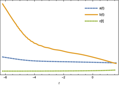
Figure 1: Evolution of the scale factors for Bianchi type IX from Kasner-like initial conditions towards the singularity. The universe contains isotropic ($\rho>0$) ultra-stiff fluid only and no anisotropic pressure field included,

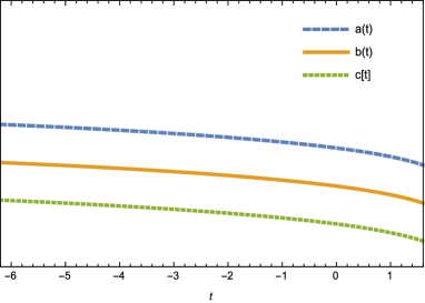
Figure 2: Evolution of the scale factors for a Bianchi type IX universe from Kasner-like initial conditions towards the singularity. The universe contains an ultra-stiff isotropic fluid ($\rho>0$) and a fluid with anisotropic pressure.

On examining Figure 1 and Figure 2, we observe the following features. The initial conditions used do not satisfy the Friedmann constraint and therefore later on in this section, the equations are solved again with initial conditions that do satisfy this constraint. There is more than one branch of solutions but at least one of the scale factors approaches the singularity in a slightly oscillatory manner as predicted in [46], while one of them stays nearly constant. On inclusion of the anisotropic energy density, the solutions seem to tend towards a contraction to a collapse, a fact that will be further verified in the case which takes into account the Friedmann constraint while picking initial conditions. In order to study the evolution of the shear and the near-singularity behaviours of the scale factors and the Hubble rates, we try to find initial conditions that satisfy the Friedmann constraint (38) and take into consideration the curvature and the matter content of the spacetime. Accordingly, we choose,

$\begin{array}[]{c|c|c|c|c|c|c|c}\hline\cr x(\tau_{0})&y(\tau_{0})&H(\tau_{0})&\alpha(\tau_{0})&\beta(\tau_{0})&\delta(\tau_{0})&\rho(\tau_{0})&\mu(\tau_{0})\\ \hline\cr m_{1}^{\prime}-m_{2}^{\prime}&m_{1}^{\prime}-m_{3}^{\prime}&(m_{1}^{\prime}+m_{2}^{\prime}+m_{3}^{\prime})/3&m_{1}&m_{2}&m_{3}&-s&v\\ \hline\cr\end{array}$ where $m_{1}^{\prime}=0.594778,m_{2}^{\prime}=0.167825,m_{3}^{\prime}=0.276172,m_{1}=1.19144,m_{2}=2.24155,m_{3}=1.22871,s=0.2175397$, and $v=0.20$; $\tau_{0}$ is the initial instant of time. For the present case, we have chosen $\tau_{0}=1.6$. The equations are evolved from $t=\tau_{f}$ to $\tau_{0}=1.6$, where $\tau_{f}=-25$. These initial conditions satisfy the Friedmann constraint (38) with an error of only $\epsilon\sim O(10^{-8})$.  

From the results of the numerical computation, we find the following evolutionary features:

4.1.1 Scale-factor evolution

In the figures shown, that is in Figure 3 and Figure 4, the logarithms of the scale factors (i.e., $\alpha,\beta,\delta$) have been plotted. The Figure 3 shows the evolution of the scale factors with the inclusion of only an isotropic ultra-stiff ghost field and Figure 4 shows the evolution of the scale factors with the inclusion of both the isotropic, ultra-stiff ghost field and the anisotropic pressure, which is also an ultra-stiff field and with greater average stiffness than the ghost field. In the absence of the anisotropic pressure field, we see that the scale factors undergo periodic bounces, with a phase of expansion, contraction and a turnaround. On inclusion of the anisotropic pressure field, the periodic bouncing behaviour is destroyed and the scale factor evolution seems to undergo gentle oscillations towards ultimately a collapse. One of the scale factors in the $c(t)$ direction remains almost constant throughout the evolution. We study the near-singularity behaviour in more detail by focusing on the evolution in a small time interval near to $t=0$. The Figure 5 shows the evolution of the scale factors with the inclusion of only an isotropic ultra-stiff ghost field very close to the singularity and the Figure 6 shows the evolution of the scale factors with the inclusion of both the isotropic, ultra-stiff ghost field as well as the anisotropic pressure, ultra-stiff (with greater stiffness than the ghost field) field very close to the singularity.

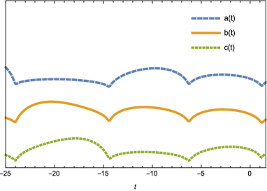
Figure 3: Scale factor evolution in Bianchi type IX with initial conditions satisfying the Friedmann constraint with isotropic ultra-stiff ghost field ($\rho<0$) and no ultra stiff anisotropic pressure field included

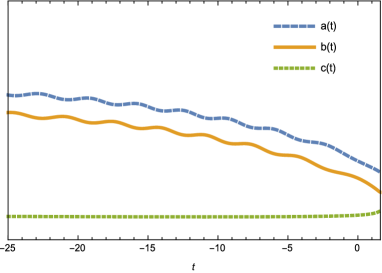
Figure 4: Scale factor evolution in Bianchi type IX with initial conditions satisfying the Friedmann constraint with isotropic ultra-stiff ghost field ($\rho<0$) and anisotropic pressure ultra-stiff field included, on approach to the singularity.

Near the singularity the solutions show the following behaviours. The scale factors for the case including only the isotropic ghost fluid do not in fact collapse to a singularity. They undergo a non-singular bounce, as expected from our experience of the isotropic closed universe and that of the Kasner universe with ghost field and radiation. However, the bounces in the three directions seem to occur almost simultaneously. It is also interesting to note that if the stiffness of the anisotropic fluid is increased, so that on the average it is stiffer than the isotropic fluid, but is not stiff in one or two directions, then the scale factors in those directions remain nearly constant. If the stiffness is less than that of the isotropic fluid, or the initial conditions are such that the ultra-stiff anisotropic fluid is negligible compared to the isotropic fluid density, they show similar behaviour to the isotropic case and undergo a bounce after which the scale factors all begin to re-expand. In all other cases, they contract until they are very near the singularity. This means that near the expected singularity, the isotropic fluid scale factors re-expand, but the scale factors in the anisotropic fluid case all seem to contract towards a singularity. In all cases, the shear for the case containing the isotropic fluid alone is lower than when the anisotropic fluid is present.

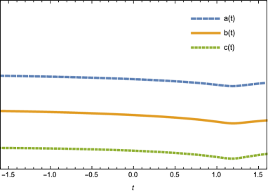
Figure 5: Scale factor evolution in Bianchi type IX near the singularity with initial conditions satisfying the Friedmann constraint with isotropic ultra-stiff ghost field ($\rho<0$) and no ultra-stiff anisotropic pressure field included.

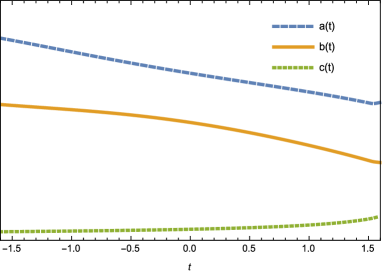
Figure 6: Scale factor evolution in Bianchi type IX near the singularity with initial conditions satisfying the Friedmann constraint with isotropic ultra-stiff ghost field ($\rho<0$) and ultra-stiff anisotropic pressure field included.

4.1.2 Shear tensor

We had initially set out to investigate the effect of the anisotropic pressure fluid on the evolution of the anisotropies. Thus, we next look at the behaviour of the shear tensor on approach to the singularity (or bounce). The shear tensor in the Bianchi type IX spacetime is given as,

$$\sigma^{2}=\frac{1}{6}\left\{(H_{\alpha}-H_{\beta})^{2}+(H_{\beta}-H_{\delta})^{2}+(H_{\delta}-H_{\alpha})^{2}\right\},$$ (43)

where $H_{\alpha}=\dot{\alpha}$, $H_{\beta}=\dot{\beta}$ and $H_{\delta}=\dot{\delta}$. We focus on the near-singularity behaviour of the shear tensor. This evolution is shown in Figure 7. On examining the figure, we find that with only the isotropic fluid present, the shear remains at a very small and nearly constant positive value. However, when we include the anisotropic pressure fluid, the shear rises and keeps rising to increasingly positive values until the singularity is reached. This is true as long as the anisotropic pressure in at least one direction is less stiff than the pressure of the isotropic ghost fluid. This is equivalent to the requirement that one third of the equation of state parameters $\gamma_{i}$ be less than the overall equation of state parameter of the isotropic ultra-stiff ghost fluid. Thus, although the anisotropic fluid may be ultra-stiff and stiffer than the isotropic fluid, it may not be stiffer in a particular direction. This causes the assumption that an energy source that behaves like ultra-stiff matter suppresses the anisotropies near the singularity in a contracting universe to break down. If the anisotropic pressures are stiffer than the isotropic pressure in all three directions ($\gamma_{i}/3>\gamma$ for all $i=1,2,3$) then the anisotropic stress is more greatly suppressed when the anisotropic pressure fluid is included compared to when only the ghost isotropic fluid is present. This is expected because it is simply the standard ekpyrotic model with a stiffer fluid present in all three scale factor directions to suppress the anisotropic stress. However, when the anisotropic pressure fields have equations of state in each direction ensuring that the anisotropic stress is not suppressed, then the universe fails to undergo a bounce and re-expansion beyond the contracting phase. Instead, the contraction accelerates towards a collapse singularity in the Weyl curvature.

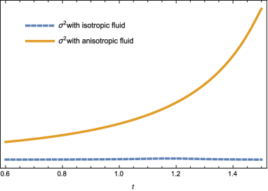
Figure 7: Evolution of the shear in a Bianchi type IX universe with initial conditions satisfying the Friedmann constraint near the singularity.

In addition to observing these trends, we also note the following general features. When the stiffness of the anisotropic fluid is less than the stiffness of the isotropic ghost fluid, the three scale factors all undergo bounces. The stiffness of the anisotropic fluid determines when this bounce occurs. If it becomes stiff on average ($\gamma_{\star}=2$), the scale factors begin to oscillate on approach to the singularity. When the anisotropic fluid is ultra-stiff on average (stiffer than the isotropic ghost fluid), but its initial conditions are such that its density is negligible or very small (less than half of the initial isotropic energy density) the scale factors begin to show a turnaround at an expansion minimum. The point of bounce is pushed towards the value at which the turnaround occurs for the isotropic case, as the anisotropic energy density is decreased.

5 Conclusions

The question of the growth of anisotropies in a contracting universe is a challenge for cyclic theories of cosmology if they aim to replicate the successes of the inflationary paradigm in explaining the present large-scale isotropy of the universe. There are several types of anisotropy that need to be investigated in order to ascertain the viability of cyclic cosmologies: simple expansion rate anisotropy, spatial curvature anisotropy, and pressure anisotropy. Simple expansion-rate anisotropies and 3-curvature anisotropies can always be dominated by an ultra-stiff perfect fluid with equation of state $p>\rho$. This is well appreciated and we confirm it here for the Bianchi class A and type IX universes. In this paper, we have focussed on the effects of pressure anisotropies in simple ekpyrotic [14, 25, 35] cyclic universe scenarios that are more general and complicated than those first studied by Barrow and Yamamoto [18]. Pressure anisotropies have been ignored in all other studies of ekpyrotic and cyclic universes. It is important to include them in the discussion because collisionless particles will be abundant near the Planck scale where graviton production is rapid and asymptotically-free interactions will not be in equilibrium. In addition, we find that if the average anisotropic pressure is allowed to exceed the energy density, just as the isotropic pressure does in the ekpyrotic scenario, then an isotropic singularity (or bounce) will be unstable unless the isotropic density is overwhelmingly larger than the anisotropic density. The anisotropic ultra-stiff fluid will drive a contracting universe to an anisotropic singularity. Evolution from cycle to cycle will accumulate anisotropic distortions to the dynamics.

More formally, we find that the anisotropy, even in the simplest case of a Bianchi I universe with anisotropic pressures present, cannot be expressed simply as a simple power-law evolution of the mean scale factor. Using a phase-space analysis for the general field equations for the Bianchi Class A group of cosmologies, we find that the presence of an ultra-stiff fluid with anisotropic pressures prevents the isotropic Friedmann-Lemaître universe from being an attractor for the initially contracting universe. More specifically, we analysed the field equations in the case of the Bianchi IX universe. We solved these equations numerically containing ultra-stiff fluids with both anisotropic and isotropic (ghost) pressures. The anisotropies grow when an anisotropic pressure fluid with dominant stiffness is included: the universe contracts and hits a singularity. This contrasts with the case containing only the isotropic ghost fluid, where the universe undergoes a non-singular bounce. Our results confirm that the inclusion of anisotropic pressures is essential in any general analysis of cyclic cosmologies and their behaviour in the presence of deviations from perfect expansion isotropy. They will be an important factor to consider in all future iterations of the cyclic universe scenario in its several forms.

Acknowledgements JDB is supported by the STFC. CG is supported by the Jawaharlal Nehru Memorial Trust Cambridge International Scholarship. The authors thank the referees for their very helpful comments, which have helped improve the current work considerably.

Appendix A Orthonormal frame formalism and the Bianchi Class A models

In this section we review the classification of the Bianchi cosmologies as given in [33]. The problem of classification of the Bianchi cosmologies can be seen as the problem of classifying the structure constants $C^{\mu}_{\alpha\beta}$ of the Lie algebra formed by the Killing vector fields(KVFs). These structure constants can be decomposed into a $2$-index symmetric object $\hat{n}_{\alpha\beta}$ and a $1$-index object $\hat{a}_{\alpha}$ as follows,

$$C^{\mu}_{\alpha\beta}=\epsilon_{\alpha\beta\nu}\hat{n}^{\mu\nu}+\hat{a}_{\alpha}\delta_{\beta}^{\mu}-\hat{a}_{\beta}\delta_{\alpha}^{\mu}$$ (44)

such that $\hat{n}^{\mu\nu}=\hat{n}^{\nu\mu}$ and $\hat{a}^{\alpha}$ are constants. They also follow the identity,

$$\hat{n}^{\alpha\beta}\hat{a}_{\beta}=0$$ (45)

The Lie algebras can thus be divided into Class A for $\hat{a}_{\alpha}=0$ and Class B for $\hat{a}_{\alpha}\neq 0$. In the standard language of the orthonormal frame formalism, we can define a unit timelike vector field u and the projection tensor $h_{ab}$ which at each point projects into the space orthogonal to the unit timelike vector field. This projection tensor is given by,

$$h_{ab}=g_{ab}+u_{a}u_{b}$$ (46)

The covariant derivative of the timelike vector field can be divided into its irreducible parts,

$$u_{a;b}=\sigma_{ab}+\omega_{ab}+\frac{1}{3}\Theta h_{ab}-\dot{u}_{a}u_{b}$$ (47)

where $\sigma_{ab}$ is the symmetric trace free, rate of shear tensor, $\omega_{ab}$ is the vorticity tensor and is antisymmetric, $\Theta$ is the rate of expansion scalar and $\dot{u}_{a}$ is the acceleration vector. Relative to a group invariant orthonormal frame given by the unit normal to the group orbits and the basis vectors $\{\textbf{n},\textbf{e}_{\alpha}\}$, the EFEs are given above in equations (12), (13), (14) and (17). The Jacobi identities are equation (14) and the following equations,

$$\dot{n}_{\alpha\beta} =-Hn_{\alpha\beta}+2\sigma_{(\alpha}^{\mu}n_{\beta)\mu}+2\epsilon_{(\alpha}^{\mu\nu}n_{\beta)\mu}\Omega_{\nu}$$ (48)

$$\dot{a}_{\alpha} =-Ha_{\alpha}-\sigma^{\beta}_{\alpha}a_{\beta}+\epsilon_{\alpha}^{\mu\nu}a_{\mu}\Omega_{\nu}$$ (49)

$$n_{\alpha}^{\beta}a_{\beta} =0$$ (50)

where $\Omega_{\nu}$ is the local angular velocity of the spatial frame with respect to the Fermi propagated spatial frame and can be expressed in terms of the components of the timelike vector field u as,

$$\Omega^{\alpha}=\frac{1}{2}\epsilon^{\alpha\mu\nu}e_{\mu}^{i}e_{\nu i;j}u^{j}$$ (51)

For our purposes, we have specialised to the case where the total stress energy tensor(isotropic stress energy tensor $+$ anisotropic part) is diagonal. Thus the more general case would include off diagonal elements of $P_{ab}$ as well and in this case $\Omega_{\nu}\neq 0$. In our case however, we need only be concerned with universes where $\Omega_{\nu}=0$.

The spatial curvature terms can be defined as,

$${}^{3}S_{\alpha\beta} =b_{\alpha\beta}-\frac{1}{3}(b^{\mu}_{\mu})\delta^{\alpha}_{\beta}-2\epsilon^{\mu\nu}_{(\alpha}n_{\beta)\mu}a_{\nu}$$ (52)

$${}^{3}R =-\frac{1}{2}b_{\mu}^{\mu}-6a_{\mu}a^{\mu}$$

where,

$$b_{\alpha\beta}=2n_{\alpha}^{\mu}n_{\mu\beta}-(n_{\mu}^{\mu})n_{\alpha\beta}$$ (53)

Appendix B New exact solution for $p=3\rho$ fluid in Bianchi I spacetime

The field equations for the Bianchi I type spacetime are:

$$\ddot{\alpha}+\dot{\alpha}^{2}+\ddot{\beta}+\dot{\beta}^{2}+\dot{\alpha}\dot{\beta} = -p,$$ (54)

$$\ddot{\beta}+\dot{\beta}^{2}+\ddot{\delta}+\dot{\delta}^{2}+\dot{\beta}\dot{\delta} = -p,$$ (55)

$$\ddot{\delta}+\dot{\delta}^{2}+\ddot{\alpha}+\dot{\alpha}^{2}+\dot{\delta}\dot{\alpha} = -p,$$ (56)

$$\dot{\alpha}\dot{\beta}+\dot{\beta}\dot{\delta}+\dot{\delta}\dot{\alpha} = \rho,$$ (57)

where the scale factors are expressed as $a(t)=\exp({\alpha(t))}$, $b(t)=\exp({\beta(t))}$, and $c(t)=\exp({\delta(t))}$. Adding equations ((54))-((56)), we get

$$2(\ddot{\alpha}+\ddot{\beta}+\ddot{\delta})+2(\dot{\alpha}^{2}+\dot{\beta}^{2}+\dot{\delta}^{2})+(\dot{\alpha}\dot{\beta}+\dot{\beta}\dot{\delta}+\dot{\delta}\dot{\alpha})=-3p.$$ (58)

Using the formula $(a+b+c)^{2}=a^{2}+b^{2}+c^{2}+2(ab+bc+ca)$, we get,

$$2(\ddot{\alpha}+\ddot{\beta}+\ddot{\delta})+2(\dot{\alpha}+\dot{\beta}+\dot{\delta})^{2}-4(\dot{\alpha}\dot{\beta}+\dot{\beta}\dot{\delta}+\dot{\delta}\dot{\alpha})+(\dot{\alpha}\dot{\beta}+\dot{\beta}\dot{\delta}+\dot{\delta}\dot{\alpha})=-3p.$$ (59)

Now substituting Equation (57) we get,

$$2(\ddot{\alpha}+\ddot{\beta}+\ddot{\delta})+2(\dot{\alpha}+\dot{\beta}+\dot{\delta})^{2}-3\rho=-3p.$$ (60)

Defining the volume as $V\equiv\exp({A)}$ where $A=(\alpha+\beta+\delta)$ we get,

$$\ddot{V}=3\rho_{0}V^{-3}.$$ (61)

Solving this gives

$$V^{2}=C_{1}t^{2}+C_{2}t+C_{3}.$$ (62)

Subtracting equations ((54)) and ((55)) we get, for example,

$$\ddot{\alpha}-\ddot{\beta}+3\dot{A}(\dot{\alpha}-\dot{\beta})=0,$$ (63)

and cyclic permutations. Thus we see that each of these combinations go as $V^{-1}$. We can write then, by integrating the above,

$$\alpha-\beta=2l_{1}\mathrm{log}[\sqrt{t}+\sqrt{C_{2}+t}],$$ (64)

and

$$\alpha-\delta=2l_{2}\mathrm{log}[\sqrt{t}+\sqrt{C_{2}+t}],$$ (65)

where $C_{1}=1,C_{3}=0$. We already know that

$$(\alpha+\beta+\delta)=\frac{1}{2}\mathrm{log}[t^{2}+C_{2}t].$$ (66)

By using the fact that $3\alpha=(\alpha+\beta+\delta)+(\alpha-\beta)+(\alpha-\delta)$, we obtain,

$$3\alpha=\mathrm{log}\left[(t^{2}+C_{2}t)^{1/2}(\sqrt{t}+\sqrt{C_{2}+t})^{2(l_{1}+l_{2})}\right].$$ (67)

Thus,

$$a(t)=\left((t^{2}+C_{2}t)^{1/2}(\sqrt{t}+\sqrt{C_{2}+t})^{2(l_{1}+l_{2})}\right)^{1/3},$$ (68)

$$b(t)=\left((t^{2}+C_{2}t)^{1/2}(\sqrt{t}+\sqrt{C_{2}+t})^{2(l_{2}-2l_{1})}\right)^{1/3},$$ (69)

$$c(t)=\left((t^{2}+C_{2}t)^{1/2}(\sqrt{t}+\sqrt{C_{2}+t})^{2(l_{1}-2l_{2})}\right)^{1/3}.$$ (70)

From the Friedmann constraint equation at late times (where $\rho\rightarrow 0$), we get the following constraint,

$$l_{1}^{2}+l_{2}^{2}-l_{1}l_{2}=1.$$ (71)

We label the indices in the solutions for the scale factors as follows,

$$3q_{1} = 1+l_{1}+l_{2},$$ (72)

$$3q_{2} = 1+l_{2}-2l_{1},$$ (73)

$$3q_{3} = 1+l_{1}-2l_{2}.$$ (74)

Therefore, we have the full solution:

$$a(t)=\left((t^{2}+C_{2}t)^{1/2}(\sqrt{t}+\sqrt{C_{2}+t})^{2(3q_{1}-1)}\right)^{1/3},$$ (75)

$$b(t)=\left((t^{2}+C_{2}t)^{1/2}(\sqrt{t}+\sqrt{C_{2}+t})^{2(3q_{2}-1)}\right)^{1/3},$$ (76)

$$c(t)=\left((t^{2}+C_{2}t)^{1/2}(\sqrt{t}+\sqrt{C_{2}+t})^{2(3q_{3}-1)}\right)^{1/3}.$$ (77)

We see that at early times this solution tends to the flat Friedmann solution for $p=3\rho$ fluid ($a\sim t^{1/6}$, $b\sim t^{1/6}$, $c\sim t^{1/6}$) as $t\rightarrow 0$, and at late times approaches the vacuum Kasner solution $a\sim t^{q_{1}}$, $b\sim t^{q_{2}}$ and $c\sim t^{q_{3}},$with $\sum_{i}q_{i}=1=\sum_{i}q_{i}^{2}$, as $t\rightarrow\infty.$ These facts can be seen to be true from equations (72) to (74) and from equation(71) respectively. Thus, this solution provides a simple exact description of the transition from an isotropic initial state to a Kasner-like anisotropic future in a particular case. It displays the opposite evolutionary trend to the evolution of a $0\leq p<\rho$ perfect-fluid model.

Appendix C Fixed points

In order to perform the stability analysis on the Bianchi Class A system, we need to identify the fixed points of the system. They have been presented in a tabular form in Table 1. The explicit forms of the relevant fixed points are given below.

$$\Sigma_{\!{}_{P_{II}}}^{\!{}^{(1)}}=\frac{1}{8}(3\gamma-2)$$

$$n_{P_{II}}^{(1)}=\frac{3}{4}[(2-\gamma)(3\gamma-2)]^{1/2},$$

$$\Omega_{P_{II}}^{(1)}=\frac{3}{16}(\gamma-6),$$

$$\Sigma_{PVI}^{(1)}=-\frac{1}{4}(3\gamma-2)$$

$$n_{PVI}^{(1)}=\pm\frac{3}{4}\sqrt{(2-\gamma)(3\gamma-2)}$$

$$\Omega_{PVI}^{(1)}=-\frac{3}{4}(2-\gamma)$$

$$t\Sigma_{\!{}_{K-}}^{\!{}^{2}}+\Sigma_{\!{}_{K+}}^{\!{}^{2}}=1$$

$$\Sigma_{\mathcal{A}_{1}}^{2}=\frac{4(\mathcal{P}_{+}^{2}+\mathcal{P}_{-}^{2})}{(\gamma_{\star}-2)^{2}}$$

$$\Sigma_{+}^{\mathcal{A}_{2}}=\frac{1}{2}\frac{\mathcal{P}_{+}(\gamma-\gamma_{\star})}{\mathcal{P}_{+}^{2}+\mathcal{P}_{-}^{2}}$$

$$\Sigma_{-}^{\mathcal{A}_{2}}=\frac{1}{2}\frac{\mathcal{P}_{-}(\gamma-\gamma_{\star})}{\mathcal{P}_{+}^{2}+\mathcal{P}_{-}^{2}}$$

$$\Omega^{\mathcal{A}_{2}}=-1+\frac{1}{4}\frac{(2-\gamma_{\star})(\gamma-\gamma_{\star})}{\mathcal{P}_{+}^{2}+\mathcal{P}_{-}^{2}}$$

$$Z^{\mathcal{A}_{2}}=\frac{1}{4}\frac{(2-\gamma)(\gamma-\gamma_{\star})}{\mathcal{P}_{+}^{2}+\mathcal{P}_{-}^{2}}$$

On examination of the forms of the fixed points, we find that only the FL, Kasner and the $\mathcal{A}_{1}$ and $\mathcal{A}_{2}$ points are physical for the case considered, that is, for ultra stiff fields, with $\gamma>2$.

Appendix D Equations for the Bianchi IX numerical computation

In Section 4, a new system of variables was introduced to make the numerical computation of the system of Einstein’s equations simpler by reducing them to first-order differential equations. They are written explicitly as follows. In all of the following $\{x,y,H,\alpha,\beta,\delta,\rho,\mu\}$ are functions of time $t$.

$$x^{\prime}+3Hx=\left(\gamma_{1}-\gamma_{2}\right)\mu+e^{-2\beta}-e^{-2\alpha}+e^{-2\delta}\left(e^{2(\beta-\alpha)}-e^{2(\alpha-\beta)}\right)$$ (78)

$$y^{\prime}+3Hy=(\gamma_{1}-\gamma_{3})\mu-e^{-2\alpha}+e^{-2\delta}+e^{-2\beta}\left(e^{2(\delta-\alpha)}-e^{2(\alpha-\delta)}\right)$$ (79)

$$6(H^{\prime}+3H^{2})=3\left(2-\gamma\right)\rho+3\left(2-\gamma_{\star}\right)\mu-2e^{-2\alpha}-2e^{-2\beta}-2e^{-2\delta}$$ (80)

$$+e^{2(\alpha-\beta-\delta)}+e^{2(\beta-\alpha-\delta)}+e^{2(\delta-\alpha-\beta)}$$

$$\rho^{\prime}=-3\gamma H\rho,\\$$

$$\mu^{\prime}=-3\mu H-\frac{(\gamma_{1}-1)}{3}(x+y+3H)\mu-\frac{(\gamma_{2}-1)}{3}(3H-2x+y)\mu$$ (81)

$$-\frac{(\gamma_{3}-1)}{3}(x-2y+3H)\mu$$

$$\alpha^{\prime}=\frac{1}{3}(3H+x+y),\\$$

$$\beta^{\prime}=\frac{1}{3}(3H-2x+y),\\$$

$$\delta^{\prime}=\frac{1}{3}(3H+x-2y).\\$$

References

- [1] Lemaître A G 1997 Gen. Rel. Gravitation 29 641
- [2] Tolman C 1931 Phys. Rev. 38 1758
- [3] Barrow J D and Da̧browski M 1995 Mon. Not. Roy. astron. Soc. 275 850
- [4] Battefeld D and Peter P 2015 Phys. Reports 571 1
- [5] Gasperini M and Veneziano G 2002 Phys. Reports 373 250
- [6] Creminelli P, Nicolis A and Trincherini E 2010 JCAP 09 021
- [7] Singh P, Vandersloot K, and Vereshchagin G V 2006 Phys. Rev. D 74 1
- [8] Casadio R 2009 Int. J. Mod. Phys. D 09 511
- [9] Acacio de Barros J, Pinto-Neto N and Sagioro-Leal M A 1998 Phys. Letters A 241 229
- [10] Barrow J D, Kimberly D and Magueijo J 2004 Class. Quantum Grav. 21 4289
- [11] Barrow J D and Sloan D 2013 Phys. Rev. D 88 023518
- [12] Barrow J D and Tsagas C G 2009 Class. Quantum Grav. 26 195003
- [13] Lehners J L 2008 Phys. Reports 465 223
- [14] Khoury J, Ovrut B A, Steinhardt P J and Turok N 2001 JHEP 11 41
- [15] Buchbinder E I, Khoury J and Ovrut B A 2007 Phys. Rev. D 76 1
- [16] Lukash V N and Starobinsky A A 1974 Sov. Phys. JETP 39 742
- [17] Barrow J D 1997 Phys. Rev. D 55 7451
- [18] Barrow J D and Yamamoto K 2010 Phys. Rev. D 82 1
- [19] Donagi R Y, Khoury J, Ovrut B A,Steinhardt P J and Turok N 2001 JHEP 11 041
- [20] Kallosh R, Kofman L, and Linde A 2001 Phys. Rev. D 64 123523
- [21] Kallosh R, Kofman L, Linde A and Tseytlin A 2001 Phys. Rev. D 64 123524
- [22] Martin J, Peter P, Pinto-Neto N and Schwarz D J 2003 Phys. Rev. D 67 028301
- [23] Steinhardt P J and Turok N 2002 Science 296 1436
- [24] Steinhardt P J and Turok N 2002 Phys. Rev. D 65 126003
- [25] Khoury J, Ovrut B A, Seiberg N, Steinhardt P J and Turok N 2002 Phys. Rev. D 65 086007
- [26] Ade P et al: BICEP2/KECK, Planck collaborations 2015 Phys. Rev. Lett. 114 101301
- [27] Brandenberger R H 2015 arXiv:1505.02381
- [28] Cai Y-F, McDonough E, Duplessis F and Brandenberger H 2013 JCAP 10 24
- [29] Coley A A and Lim W C 2005 Class.Quant.Grav. 22 3073
- [30] Barrow J D and Matzner R A 1977 Mon. Not. Roy. astron. Soc. 181 719
- [31] Kasner E 1921 Amer. J. Math. 43 217
- [32] Taub A H 1951 Ann. Math. 53 472
- [33] Wainwright J and Ellis G F R 1997 Dynamical Systems in Cosmology (Cambridge: Cambridge UP) p 123
- [34] Ellis G F R and MacCallum M A H 1969 Commun. Math. Phys. 12 108
- [35] Erickson J K, Wesley D H, Steinhardt P J and Turok N 2004 Phys. Rev. D 69 1
- [36] Calogero S and Heinzle J M 2011 Physica D 240 636
- [37] Lidsey J E 2005 Class. Quantum Grav. 23 3517
- [38] Barrow J D and Sonoda D H 1986 Phys. Reports 139 1
- [39] Misner C W 1969 Phys. Rev. Lett. 22 1071
- [40] Carrasco J J M, Chemissany W and Kallosh R 2013 arXiv:1311.3671 JHEP
- [41] Bars I 2012 arXiv:1209.1068
- [42] Belinskii V A, Khalatnikov I M and Lifshitz E M 1970 Adv. Phys. 19 525
- [43] Landau L D and Lifshitz E M 1974 The Classical Theory of Fields (Oxford: Pergamon Press) 4th rev edn
- [44] Chernoff D and Barrow J D 1983 Phys. Rev. Lett. 50 134
- [45] Barrow J D 1984 in Classical General Relativity, eds. Bonnor W, Islam J and MacCallum M A H, (Cambridge: CUP) pp 25-41
- [46] Belinski V A and Khalatnikov I M 1972 Zhurnal Eksperimental Teor. Fiz. 63 1121
- [47] Matzner R A, Ryan M P and Toton E 1973 Nuovo Cimento B 148 161
- [48] Barrow J D 1978 Nature 272 211
- [49] Demaret J M, Henneaux M and Spindel P 1985 Phys. Lett. B 164 27