Viable Control of an Epidemiological Model

Michel De Lara111Université Paris-Est, CERMICS (ENPC), 6-8 Avenue Blaise Pascal, Cité Descartes, 77455 Marne-la-Vallée, France, delara@cermics.enpc.fr    Lilian Sofia Sepulveda Salcedo 222Universidad Autónoma de Occidente, Km. 3 vía Cali-Jamundí, Cali, Colombia, lssepulveda@uao.edu.co
Abstract

In mathematical epidemiology, epidemic control often aims at driving the number of infected individuals to zero, asymptotically. However, during the transitory phase, the number of infected can peak at high values. In this paper, we consider mosquito vector control in the Ross-Macdonald epidemiological model, with the goal of capping the proportion of infected by dengue at the peak. We formulate this problem as one of control of a dynamical system under state constraint. We allow for time-dependent fumigation rates to reduce the population of mosquito vector, in order to maintain the proportion of infected individuals by dengue below a threshold for all times. The so-called viability kernel is the set of initial states (mosquitoes and infected individuals) for which such a fumigation control trajectory exists. Depending on whether the cap on the proportion of infected is low, high or medium, we provide different expressions of the viability kernel. We also characterize so-called viable policies that produce, at each time, a fumigation rate as a function of current proportions of infected humans and mosquitoes, such that the proportion of infected humans remains below a threshold for all times. We provide a numerical application in the case of control of a dengue outbreak in 2013 in Cali, Colombia.

Keywords: epidemiology; control theory; viability theory; Ross-Macdonald model; dengue.

1 Introduction

We consider vector control of the spread of an epidemic transmitted by vector in a Ross-Macdonald model. Our approach aims at controlling the number infected at the peak: we look for a trajectory of time-dependent vector mortality rates that is able to maintain the number of infected individuals below a threshold for all times. This approach differs from the widespread stationary control strategies, based upon having control reproductive number stricly less than one to ensure convergence, and also from cost minimization optimal control ones.

Indeed, many studies on mathematical modeling of infectious diseases consist of analyzing the stability of the equilibria of a differential system (behavioral models such as SIR, SIS, SEIR [9]). Those studies focus on asymptotic behavior and stability, generally leaving aside the transient behavior of the system, where the infection can reach high levels. In many epidemiological models, a significant quantity is the “basic reproductive number” 0subscript0{\cal R}_{0} which depends on parameters such as the transmission rate, the death and birth rate, etc. Numerous works (see references in [19, 14]) exhibit conditions on 0subscript0{\cal R}_{0} such that the number of infected individuals tends towards zero. With this tool, different (time-stationary) management strategies of the propagation of the infection – quarantine, vaccination, etc. – are compared with respect to how they modify 0subscript0{\cal R}_{0}. Thus, strategies are compared as to their capacity to drive the number of infected towards zero, focusing on asymptotics. However, during the transitory phase, the number of infected can peak at high values.

Other works deal with the whole trajectory, as in dynamic optimization where strategies are compared with respect to intertemporal costs and benefits [20], [23], [18], [22], [12], etc. More recently, [17] studies controls that minimize the outbreak size (or infectious burden) under the assumption that there are limited control resources.

Our approach focuses both on transitories and asymptotics, in a robust way. Instead of aiming at an equilibrium or optimizing, we look for policies able to maintain the infected individuals below a threshold for all times. To our knowledge, this approach is new in mathematical epidemiology. We have only found it mentioned in passing in [20] as a constraint – bounding above the maximum number infected at the peak – in a dynamic optimization problem, solved numerically.

In this paper, we formulate the problem as one of viability. In a nutshell, viability theory examines when and how can the state of a control system can be maintained within a given region for all times [2]. Such problems of dynamic control under constraints also refer to invariance issues [10]. In the control theory literature, problems of constrained control lead to the study of positively invariant sets, particularly ellipsoidal and polyhedral ones for linear systems (see[5], [15], [16] and the survey paper [6]); reachability of target sets or tubes for nonlinear discrete time dynamics is examined in [4]. In continuous time, such a viability approach has been applied to models related to the sustainable management of fisheries [3], to viable strategies to ensure survival of some species [8], to secure the prey predator system [7], etc. In discrete-time, different examples can be found in [13] for sustainable management applications of viability.

The paper is organized as follows. In Section 2, we state the viability problem for the Ross-Macdonald model with control on the mosquito population by requiring to keep the proportion of infected humans below a given threshold. The viability kernel is the set of initial states such that there exists at least one fumigation control trajectory such that the resulting proportion of infected humans remains below a given threshold for all times. In Section 3, we provide a characterization of the viability kernel depending on whether the cap for the proportion of infected humans is low, high or medium. We also discuss viable controls. We apply our theoretical results to the case of the dengue outbreak in 2013 in Cali, Colombia. Thanks to numerical data provided by the Municipal Secretariat of Public Health of Cali, we provide figures of viability kernels and of viable trajectories.

2 The viability problem

First, we present the Ross-MacDonald model. Second, we formulate the viability problem, which consists in capping the proportion of infected humans using the dynamics described by the Ross-MacDonald model. Then, we introduce the viability kernel and viability domains. Finally, we describe viable equilibria, that are part of the viability kernel.

2.1 The Ross-MacDonald model

Different types of Ross-MacDonald models have been published [28]. We choose the one in [1], where both total populations (humans, mosquitoes) are normalized to 1 and divided between susceptibles and infected. The basic assumptions of the model are the following.

  • i)

    The human population (Nhsubscript𝑁N_{h}) and the mosquito population (Nmsubscript𝑁𝑚N_{m}) are closed and remain stationary.

  • ii)

    Humans and mosquitoes are homogeneous in terms of susceptibility, exposure and contact.

  • iii)

    The incubation period is ignored, in humans as in mosquitoes.

  • iv)

    Death induced by the disease is ignored, in humans as in mosquitoes.

  • v)

    Once infected, mosquitoes never recover.

  • vi)

    Only susceptibles get infected, in humans as in mosquitoes.

  • vii)

    Gradual immunity in humans is ignored.

Let m(t)𝑚𝑡m(t) denote the proportion of infected mosquitoes at time t𝑡t, and h(t)𝑡h(t) the proportion of infected humans at time t𝑡t. Therefore, 1m(t)1𝑚𝑡1-m(t) and 1h(t)1𝑡1-h(t) are the respective proportions of susceptibles. The Ross-MacDonald model is the following differential system

dmdt𝑑𝑚𝑑𝑡\displaystyle\displaystyle\frac{dm}{dt} =\displaystyle= αpmh(1m)δm,𝛼subscript𝑝𝑚1𝑚𝛿𝑚\displaystyle\alpha\,p_{m}\,h(1-m)-\delta\,m\;,\enspace (1a)
dhdt𝑑𝑑𝑡\displaystyle\displaystyle\frac{dh}{dt} =\displaystyle= αphNmNhm(1h)γh,𝛼subscript𝑝subscript𝑁𝑚subscript𝑁𝑚1𝛾\displaystyle\alpha\,p_{h}\,\frac{N_{m}}{N_{h}}\,m(1-h)-\gamma\,h\;,\enspace (1b)

where the parameters α𝛼\alpha, pm,phsubscript𝑝𝑚subscript𝑝p_{m},\,p_{h}, ξ=NmNh𝜉subscript𝑁𝑚subscript𝑁\xi=\frac{N_{m}}{N_{h}}, δ𝛿\delta and γ𝛾\gamma are given in Table 1.

Parameter Description
α0𝛼0\alpha\geq 0 biting rate per time unit
ξ=Nm/Nh0𝜉subscript𝑁𝑚subscript𝑁0\xi=N_{m}/N_{h}\geq 0 number of female mosquitoes per human
1ph01subscript𝑝01\geq p_{h}\geq 0 probability of infection of a susceptible human
by infected mosquito biting
1pm01subscript𝑝𝑚01\geq p_{m}\geq 0 probability of infection of a susceptible mosquito
when biting an infected human
γ0𝛾0\gamma\geq 0 recovery rate for humans
δ0𝛿0\delta\geq 0 (natural) death rate for mosquitoes
Table 1: Parameters of the Ross-MacDonald model (1)

2.2 Capping the proportion of infected humans

We turn the dynamical system (1) into a control system by replacing the natural death rate δ𝛿\delta for mosquitoes in (1a) by a piecewise continuous function u():tu(t)[u¯,u¯]:𝑢𝑡𝑢𝑡¯𝑢¯𝑢u(\cdot):t\rightarrow u(t)\in[\underline{u},\overline{u}], with u¯=δ¯𝑢𝛿\underline{u}=\delta. The function u()𝑢u(\cdot) is the control on mosquito population that affects the mortality rate by fumigation of insecticides. The upper bound u¯¯𝑢\overline{u} is the maximal fumigation mortality rate. For notational simplicity, we put

Am=αpm,Ah=αphMH.formulae-sequencesubscript𝐴𝑚𝛼subscript𝑝𝑚subscript𝐴𝛼subscript𝑝𝑀𝐻A_{m}=\alpha p_{m}\;,\enspace A_{h}=\alpha p_{h}\frac{M}{H}\;. (2)

Thinking about public health policies set by governmental entities, we impose the following constraint: the proportion h(t)𝑡h(t) of infected humans must always remain below a threshold H¯¯𝐻\overline{H}, where

0<H¯<1,0¯𝐻10<\overline{H}<1\;,\enspace (3)

represents the maximum tolerated proportion of infected humans.

Therefore, the viability problem for the Ross-Macdonald model with control on the mosquito population is as follows. Given the control system

dmdt=𝑑𝑚𝑑𝑡absent\displaystyle\displaystyle\frac{dm}{dt}= Amh(t)(1m(t))u(t)m(t),subscript𝐴𝑚𝑡1𝑚𝑡𝑢𝑡𝑚𝑡\displaystyle A_{m}h(t)(1-m(t))-u(t)m(t)\;,\enspace (4a)
dhdt=𝑑𝑑𝑡absent\displaystyle\displaystyle\frac{dh}{dt}= Ahm(t)(1h(t))γh(t),subscript𝐴𝑚𝑡1𝑡𝛾𝑡\displaystyle A_{h}m(t)(1-h(t))-\gamma h(t)\;,\enspace (4b)

determine if there exists a piecewise continuous control trajectory u()𝑢u(\cdot) such that

u():tu(t),u¯u(t)u¯,t0,u(\cdot):t\mapsto u(t)\;,\enspace\underline{u}\leq u(t)\leq\overline{u}\;,\enspace\forall t\geq 0\;,\enspace (5)

and such that the state trajectory given by (4) satisfies the viability constraint

h(t)H¯,t0.formulae-sequence𝑡¯𝐻for-all𝑡0h(t)\leq\overline{H}\;,\enspace\forall t\geq 0\;. (6)

2.3 Viability kernel and viability domains

The solution to problem (6) relies mainly on identifying the initial conditions, (m(0),h(0))𝑚00(m(0),h(0)), for the mosquitoes and infected humans, for which there exists a mortality rate due to fumigation, u()𝑢u(\cdot) like (5), such that the solution (4) starting from (m(0),h(0))𝑚00(m(0),h(0)) satisfies (6). Such set of initial conditions is called the viability kernel.

Definition 1.

The set of initial conditions (m0,h0)subscript𝑚0subscript0(m_{0},h_{0}) for which there exists at least one fumigation policy (5) such that the solution to the system (4), with initial state (m(0),h(0))=(m0,h0)𝑚00subscript𝑚0subscript0(m(0),h(0))=(m_{0},h_{0}), satisfies the constraint (6) is called the viability kernel. We denote the viability kernel by 𝕍(H¯)𝕍¯𝐻\mathbb{V}(\overline{H}), that is,

𝕍(H¯)={(m0,h0)|there is u()as in (5)such that the solution to (4)which starts from (m0,h0)satisfies the constraint (6)}.\mathbb{V}(\overline{H})=\left\{(m_{0},h_{0})\left|\begin{array}[]{c}\textit{there is }u(\cdot)\textit{as in }~{}\eqref{eq:restriccion-control}\\ \textit{such that the solution to }~{}\eqref{eq:model-control-vector}\\ \textit{which starts from }(m_{0},h_{0})\\ \textit{satisfies the constraint }~{}\eqref{eq:restriccion-estado}\end{array}\right.\right\}\;. (7)

The viability kernel is a subset of the constraint set

𝕍0(H¯)={(m,h)|0m1,0hH¯}=[0,1]×[0,H¯],superscript𝕍0¯𝐻conditional-set𝑚formulae-sequence0𝑚10¯𝐻010¯𝐻\mathbb{V}^{0}(\overline{H})=\{(m,h)|0\leq m\leq 1,0\leq h\leq\overline{H}\}=[0,1]\times[0,\overline{H}]\;, (8)

that is,

𝕍(H¯)𝕍0(H¯).𝕍¯𝐻superscript𝕍0¯𝐻\mathbb{V}(\overline{H})\subset\mathbb{V}^{0}(\overline{H})\;. (9)

We define and present a geometric characterization of so-called viability domains of system (4), as they will be an important step to characterize the viability kernel.

Definition 2.

A subset 𝕍𝕍\mathbb{V} of the set of states [0,1]×[0,1]0101[0,1]\times[0,1] is said to be a viability domain for the system (4)–(5) if there exists a control trajectory u()𝑢u(\cdot) as in (5) such that the solution to (4), which starts from (m(0),h(0))𝕍𝑚00𝕍(m(0),h(0))\in\mathbb{V}, remains within 𝕍𝕍\mathbb{V} for every t0𝑡0t\geq 0.

Viability domains are related to the viability kernel as follows.

Theorem 3 ([2]).

The viability kernel is the largest viability domain within the constraint set.

With system (4), we associate the vector field (gm,gh)subscript𝑔𝑚subscript𝑔(g_{m},g_{h}) given by the two components

gm(m,h,u)subscript𝑔𝑚𝑚𝑢\displaystyle g_{m}(m,h,u) =Amh(1m)um,absentsubscript𝐴𝑚1𝑚𝑢𝑚\displaystyle=A_{m}h(1-m)-um\;, (10a)
gh(m,h)subscript𝑔𝑚\displaystyle g_{h}(m,h) =Ahm(1h)γh.absentsubscript𝐴𝑚1𝛾\displaystyle=A_{h}m(1-h)-\gamma h\;. (10b)

The system (4) is equivalent to

dmdt𝑑𝑚𝑑𝑡\displaystyle\displaystyle\frac{dm}{dt} =gm(m(t),h(t),u(t)),absentsubscript𝑔𝑚𝑚𝑡𝑡𝑢𝑡\displaystyle=g_{m}\big{(}m(t),h(t),u(t)\big{)}\;,\enspace (11a)
dhdt𝑑𝑑𝑡\displaystyle\displaystyle\frac{dh}{dt} =gh(m(t),h(t)).absentsubscript𝑔𝑚𝑡𝑡\displaystyle=g_{h}\big{(}m(t),h(t)\big{)}\;. (11b)

We now provide a geometric characterization of the viability domains of the system (11) with control constraints (5) using the vector field (gm,gh)subscript𝑔𝑚subscript𝑔(g_{m},g_{h}). For this purpose, we first note that the system (11) is Marchaud [2] because:

  • the constraint (5) on the controls is written as u[u¯,u¯]𝑢¯𝑢¯𝑢u\in[\underline{u},\overline{u}], where [u¯,u¯]¯𝑢¯𝑢[\underline{u},\overline{u}] is closed;

  • the components of the vector field (gm,gh)subscript𝑔𝑚subscript𝑔(g_{m},g_{h}) in (10) are continuous;

  • the vector field (gm,gh)subscript𝑔𝑚subscript𝑔(g_{m},g_{h}) and the set [u¯,u¯]¯𝑢¯𝑢[\underline{u},\overline{u}] have linear growth (because the partial derivatives of (gm,gh)subscript𝑔𝑚subscript𝑔(g_{m},g_{h}) are smooth and defined over the compact [0,1]×[0,1]0101[0,1]\times[0,1]);

  • the set {(gm,gh)(m,h,u)u[u¯,u¯]}conditional-setsubscript𝑔𝑚subscript𝑔𝑚𝑢𝑢¯𝑢¯𝑢\{(g_{m},g_{h})(m,h,u)\mid u\in[\underline{u},\overline{u}]\} is convex, for all (m,h)𝑚(m,h), because gm(m,h,u)subscript𝑔𝑚𝑚𝑢g_{m}(m,h,u) is linearly dependent on the control u𝑢u.

Second, we will use the following result to be found in [2] (Theorem 6.1.4, p. 203 and the remark p. 200).

Proposition 4.

For a Marchaud controlled system, a closed subset 𝕍𝕍\mathbb{V} is viable if the tangent cone at any point in 𝕍𝕍\mathbb{V} contains at least one of the vectors in the family generated by the vector field at this point when the control varies.

In our case, we obtain the following geometric characterization of viability domains.

Proposition 5.

Consider a closed subset 𝕍𝕍\mathbb{V} of [0,1]×[0,1]0101[0,1]\times[0,1]. The set 𝕍𝕍\mathbb{V} is a viability domain for the system (4), if, whenever (m,h)𝑚(m,h) varies along the frontier 𝕍𝕍\partial\mathbb{V} of the set 𝕍𝕍\mathbb{V}, there is a control u[u¯,u¯]𝑢¯𝑢¯𝑢u\in[\underline{u},\overline{u}] such that (gm(m,h,u),gh(m,h))subscript𝑔𝑚𝑚𝑢subscript𝑔𝑚(g_{m}(m,h,u),g_{h}(m,h)) is an inward-pointing vector, with respect to the set 𝕍𝕍\mathbb{V}.

If the closed subset 𝕍𝕍\mathbb{V} has a piecewise smooth frontier 𝕍𝕍\partial\mathbb{V}, it suffices — for the set 𝕍𝕍\mathbb{V} to be a viability domain for the system (4) — that the scalar product between the vector (gm,gh)subscript𝑔𝑚subscript𝑔(g_{m},g_{h}) and a normal (non zero) outward-pointing vector (with respect to the set 𝕍𝕍\mathbb{V}) be lower than or equal to zero.

2.4 Viable equilibria

Control systems display a family of equilibria, indexed by stationary decisions. Within them, the equilibria which satisfy the constraints are part of the viability kernel: they are said to be viable equilibria.

Stationary control: mortality rate due to constant fumigation

Consider stationary mosquito control, that is, constant mortality rate due to fumigation:

u(t)=um,t0, with u¯umu¯.formulae-sequence𝑢𝑡subscript𝑢𝑚formulae-sequencefor-all𝑡0 with ¯𝑢subscript𝑢𝑚¯𝑢u(t)=u_{m}\;,\enspace\forall t\geq 0\;,\enspace\text{ with }\underline{u}\leq u_{m}\leq\overline{u}\;. (12)

The system (4) has the disease free equilibrium (0,0)00(0,0) and, possibly, the endemic equilibrium point:

Eum=(m,h)=(Amγum/AhAm+um,Ahγum/AmAh+γ).subscriptsuperscript𝐸subscript𝑢𝑚superscript𝑚superscriptsubscript𝐴𝑚𝛾subscript𝑢𝑚subscript𝐴subscript𝐴𝑚subscript𝑢𝑚subscript𝐴𝛾subscript𝑢𝑚subscript𝐴𝑚subscript𝐴𝛾E^{*}_{u_{m}}=(m^{*},h^{*})=\displaystyle\left(\frac{A_{m}-\gamma u_{m}/A_{h}}{A_{m}+u_{m}},\frac{A_{h}-\gamma u_{m}/A_{m}}{A_{h}+\gamma}\right)\;. (13)

Such point Eumsubscriptsuperscript𝐸subscript𝑢𝑚E^{*}_{u_{m}} exists in [0,1]2superscript012[0,1]^{2} and has global asymptotic stability when

0<AmAhγum.0subscript𝐴𝑚subscript𝐴𝛾subscript𝑢𝑚0<{A_{m}A_{h}-\gamma u_{m}}\;. (14)

The proof relies on the Poincaré-Bendixson theorem, excluding periodic orbits thanks to the Bendixson-Dulac criterion [30].

The viable equilibrium points (m,h)superscript𝑚superscript(m^{*},h^{*}) are those for which hH¯superscript¯𝐻h^{*}\leq\overline{H}. With (14), we deduce that the viable equilibrium points are the points (13) for which:

0<Ahγum/AmAh+γH¯.0subscript𝐴𝛾subscript𝑢𝑚subscript𝐴𝑚subscript𝐴𝛾¯𝐻0<\frac{A_{h}-\gamma u_{m}/A_{m}}{A_{h}+\gamma}\leq\overline{H}\;. (15)

Monotonicity properties

The system (4) has monotonicity properties which will be practical for characterizing of the viability kernel.

Proposition 6.

Let (m¯(t),h¯(t))¯𝑚𝑡¯𝑡\big{(}\overline{m}(t),\overline{h}(t)\big{)} be the solution to (4) when u(t)=u¯𝑢𝑡¯𝑢u(t)=\overline{u}. If

m¯(0)m(0),h¯(0)h(0),formulae-sequence¯𝑚0𝑚0¯00\overline{m}(0)\leq m(0)\;,\enspace\overline{h}(0)\leq h(0)\;, (16)

we have that

m¯(t)m(t),h¯(t)h(t),t>0.formulae-sequence¯𝑚𝑡𝑚𝑡formulae-sequence¯𝑡𝑡for-all𝑡0\overline{m}(t)\leq m(t)\;,\enspace\overline{h}(t)\leq h(t)\;,\enspace\forall t>0\;. (17)
Proof.

Note that the components of vector field (gm,gh)subscript𝑔𝑚subscript𝑔(g_{m},g_{h}) in (10) are smooth, and that, when (m,h)[0,1]2𝑚superscript012(m,h)\in[0,1]^{2},

gmh=Am(1m)0,ghm=Ah(1h)0.formulae-sequencesubscript𝑔𝑚subscript𝐴𝑚1𝑚0subscript𝑔𝑚subscript𝐴10\frac{\partial g_{m}}{\partial h}=A_{m}(1-m)\geq 0\;,\enspace\frac{\partial g_{h}}{\partial m}=A_{h}(1-h)\geq 0\;. (18)

By Definition 15 of Appendix A.1, (gm,gh)subscript𝑔𝑚subscript𝑔(g_{m},g_{h}) is quasi monotonous in (m,h)𝑚(m,h) for any control tu(t)maps-to𝑡𝑢𝑡t\mapsto u(t).

Denote by (gm¯,gh¯)¯subscript𝑔𝑚¯subscript𝑔(\overline{g_{m}},\overline{g_{h}}) the vector fields when u=u¯𝑢¯𝑢u=\overline{u} and u¯¯𝑢\underline{u}, respectively, in (10). Since gm¯gm¯subscript𝑔𝑚subscript𝑔𝑚\overline{g_{m}}\leq g_{m} and gh¯gh¯subscript𝑔subscript𝑔\overline{g_{h}}\leq g_{h}, through the comparison Theorem 17, we obtain the following the result: if m¯(0)m(0)¯𝑚0𝑚0\overline{m}(0)\leq m(0) and h¯(0)h(0)¯00\overline{h}(0)\leq h(0), then m¯(t)m(t)¯𝑚𝑡𝑚𝑡\overline{m}(t)\leq m(t) and h¯(t)h(t)¯𝑡𝑡\overline{h}(t)\leq h(t), for every t0𝑡0t\geq 0. ∎

3 Characterization of the viability kernel

We will show that the characterization of the viability kernel (7) depends on whether the upper limit H¯¯𝐻\overline{H} for the proportion of infected humans in (6) is low, high or medium.

L)

When H¯¯𝐻\overline{H} is low in (6), a strong constraint is put on the proportion of infected humans, and we will prove in §3.1 that the viability kernel (7) reduces to the origin {(0,0)}00\{(0,0)\}.

H)

When H¯¯𝐻\overline{H} is high in (6), hence allowing the proportion of infected humans to be large, the viability kernel is the entire constraint set 𝕍0(H¯)superscript𝕍0¯𝐻\mathbb{V}^{0}(\overline{H}) in (8), as we will show in §3.2.

M)

Finally, when H¯¯𝐻\overline{H} is medium in (6), which is a more interesting case, the viability kernel (7) is a strict subset of the constraint set 𝕍0(H¯)superscript𝕍0¯𝐻\mathbb{V}^{0}(\overline{H}) in (8), whose upper right frontier is a smooth curve that we characterize. The proof of this result will be given in §3.3.

3.1 When the infected humans upper bound is low

When the imposed constraint (6) is strong, meaning that the upper bound H¯¯𝐻\overline{H} for the proportion of infected humans is low, the viability kernel (7) reduces to the origin {(0,0)}00\{(0,0)\} as follows.

Proposition 7.

If

H¯<Ahγu¯/AmAh+γ,¯𝐻subscript𝐴𝛾¯𝑢subscript𝐴𝑚subscript𝐴𝛾\overline{H}<\frac{A_{h}-\gamma\overline{u}/A_{m}}{A_{h}+\gamma}\;,\enspace (19)

the viability kernel (7) only consists of the origin:

𝕍(H¯)={(0,0)}.𝕍¯𝐻00\mathbb{V}(\overline{H})=\{(0,0)\}\;. (20)
Proof.

First, note that the state (0,0)00(0,0) is a viable equilibrium, as seen in §2.4. Second, if the initial conditions (m(0),h(0))𝑚00(m(0),h(0)) are taken outside {(0,0)}00\{(0,0)\}, let us show that, for any u()𝑢u(\cdot) as in (5), the solution to (4) violates the constraint (6).

Indeed, let m¯(t)¯𝑚𝑡\overline{m}(t) and h¯(t)¯𝑡\overline{h}(t) be solutions to (4) when u(t)=u¯𝑢𝑡¯𝑢u(t)=\overline{u} and with initial state (m(0),h(0))𝑚00(m(0),h(0)). The assumption (19) implies the condition (14) that makes the endemic equilibrium point

Eu¯=(mu¯,hu¯)=(Amγum/AhAm+um,Ahγum/AmAh+γ)subscriptsuperscript𝐸¯𝑢subscriptsuperscript𝑚¯𝑢subscriptsuperscript¯𝑢subscript𝐴𝑚𝛾subscript𝑢𝑚subscript𝐴subscript𝐴𝑚subscript𝑢𝑚subscript𝐴𝛾subscript𝑢𝑚subscript𝐴𝑚subscript𝐴𝛾E^{*}_{\overline{u}}=(m^{*}_{\overline{u}},h^{*}_{\overline{u}})=\displaystyle\left(\frac{A_{m}-\gamma u_{m}/A_{h}}{A_{m}+u_{m}},\frac{A_{h}-\gamma u_{m}/A_{m}}{A_{h}+\gamma}\right) (21)

exist and display global asymptotic stability, as seen in §2.4. Hence, h¯(t)¯𝑡\overline{h}(t) approaches hu¯subscriptsuperscript¯𝑢h^{*}_{\overline{u}} with H¯<hu¯¯𝐻subscriptsuperscript¯𝑢\overline{H}<h^{*}_{\overline{u}}. So, by (19) and (21), we have h¯(t)>H¯¯𝑡¯𝐻\overline{h}(t)>\overline{H} for all t𝑡t large enough.

From Proposition 6, we have that h¯(t)h(t)¯𝑡𝑡\overline{h}(t)\leq h(t), for every t0𝑡0t\geq 0, so, for a significantly large t𝑡t, we have that H¯<h¯(t)h(t)¯𝐻¯𝑡𝑡\overline{H}<\overline{h}(t)\leq h(t).

Therefore, for any initial condition outside {(0,0)}00\{(0,0)\}, for any u()𝑢u(\cdot) as in (5), the solution to (4) violates the constraint (6) for times t𝑡t large enough, hence at least for one time. ∎

3.2 When the infected humans upper bound is high

When the imposed constraint (6) is weak, meaning that the upper bound H¯¯𝐻\overline{H} for the proportion of infected humans is high, the viability kernel is the entire constraint set 𝕍0(H¯)superscript𝕍0¯𝐻\mathbb{V}^{0}(\overline{H}) in (8) as follows.

Proposition 8.

If

AhAh+γH¯,subscript𝐴subscript𝐴𝛾¯𝐻\frac{A_{h}}{A_{h}+\gamma}\leq\overline{H}\;, (22)

the constraint set 𝕍0(H¯)superscript𝕍0¯𝐻\mathbb{V}^{0}(\overline{H}) in (8) is strongly invariant and is, therefore, the viability kernel:

𝕍(H¯)=𝕍0(H¯)=[0,1]×[0,H¯].𝕍¯𝐻superscript𝕍0¯𝐻010¯𝐻\mathbb{V}(\overline{H})=\mathbb{V}^{0}(\overline{H})=[0,1]\times[0,\overline{H}]\;. (23)
Proof.

Consider the vector field (gm,gh)subscript𝑔𝑚subscript𝑔(g_{m},g_{h}) described in (10), which corresponds to the system (4). We will study the vector (gm,gh)subscript𝑔𝑚subscript𝑔(g_{m},g_{h}) along the four faces of the rectangle 𝕍0(H¯)superscript𝕍0¯𝐻\mathbb{V}^{0}(\overline{H}) and we will prove that, for any control, (gm,gh)subscript𝑔𝑚subscript𝑔(g_{m},g_{h}) is an inward-pointing vector, with respect to the set 𝕍0(H¯)superscript𝕍0¯𝐻\mathbb{V}^{0}(\overline{H}) (that is, the vector (gm,gh)subscript𝑔𝑚subscript𝑔(g_{m},g_{h}) belongs to the tangent cone, which is closed). Thanks to Proposition 4 (in fact, a time-varying extension), this suffices to prove that 𝕍0(H¯)superscript𝕍0¯𝐻\mathbb{V}^{0}(\overline{H}) is strongly invariant.

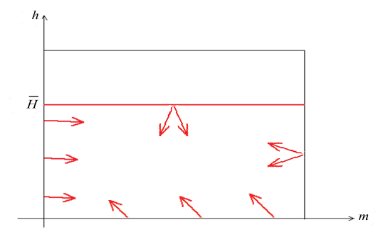
  • For any state (m,h)𝑚(m,h) on the vertical half-line m=0𝑚0m=0 and h00h\geq 0, we have that:

    gm(0,h,u)=Amh0,gh(0,h)=γh0.formulae-sequencesubscript𝑔𝑚0𝑢subscript𝐴𝑚0subscript𝑔0𝛾0g_{m}(0,h,u)=A_{m}h\geq 0\;,\enspace g_{h}(0,h)=-\gamma h\leq 0\;. (24)
    Refer to caption
    Figure 1: Vector field (gm,gh)subscript𝑔𝑚subscript𝑔(g_{m},g_{h}) on the frontier of the constraint set 𝕍0(H¯)superscript𝕍0¯𝐻\mathbb{V}^{0}(\overline{H})

    Therefore, for any control u[u¯,u¯]𝑢¯𝑢¯𝑢u\in[\underline{u},\overline{u}], the vector (gm,gh)subscript𝑔𝑚subscript𝑔(g_{m},g_{h}) always points towards the inside of 𝕍0(H¯)superscript𝕍0¯𝐻\mathbb{V}^{0}(\overline{H}) (see the left part of Figure 1).

  • For any state (m,h)𝑚(m,h) on the horizontal half-line h=00h=0 and m0𝑚0m\geq 0, we have that:

    gm(0,h,u)=um0,gh(0,h)=Ahm0.formulae-sequencesubscript𝑔𝑚0𝑢𝑢𝑚0subscript𝑔0subscript𝐴𝑚0g_{m}(0,h,u)=-um\leq 0\;,\enspace g_{h}(0,h)=A_{h}m\geq 0\;. (25)

    Therefore, for any control u[u¯,u¯]𝑢¯𝑢¯𝑢u\in[\underline{u},\overline{u}], the vector (gm,gh)subscript𝑔𝑚subscript𝑔(g_{m},g_{h}) always points towards the inside of 𝕍0(H¯)superscript𝕍0¯𝐻\mathbb{V}^{0}(\overline{H}) (see the bottom part of Figure 1).

  • For any state (m,h)𝑚(m,h) on the vertical line m=1𝑚1m=1, we have that

    gm(1,h,u)=uu¯0.subscript𝑔𝑚1𝑢𝑢¯𝑢0g_{m}(1,h,u)=-u\leq-\underline{u}\leq 0\;. (26)

    Therefore, for any control u[u¯,u¯]𝑢¯𝑢¯𝑢u\in[\underline{u},\overline{u}], the vector (gm,gh)subscript𝑔𝑚subscript𝑔(g_{m},g_{h}) always points to the left of the line m=1𝑚1m=1. Hence, the vector (gm,gh)subscript𝑔𝑚subscript𝑔(g_{m},g_{h}) always points towards the inside of 𝕍0(H¯)superscript𝕍0¯𝐻\mathbb{V}^{0}(\overline{H}) (see the right part of Figure 1).

  • Finally, for any state (m,h)𝑚(m,h) on the horizontal half-line h=H¯¯𝐻h=\overline{H} and m1𝑚1m\leq 1, we have that

    gh(m,H¯)=Ahm(1H¯)γH¯Ah(1H¯)γH¯0,subscript𝑔𝑚¯𝐻subscript𝐴𝑚1¯𝐻𝛾¯𝐻subscript𝐴1¯𝐻𝛾¯𝐻0g_{h}(m,\overline{H})=A_{h}m(1-\overline{H})-\gamma\overline{H}\leq A_{h}(1-\overline{H})-\gamma\overline{H}\leq 0\;, (27)

    by (22) (which is equivalent to Ah(1H¯)γH¯subscript𝐴1¯𝐻𝛾¯𝐻A_{h}(1-\overline{H})\leq\gamma\overline{H}). Therefore, for any control u[u¯,u¯]𝑢¯𝑢¯𝑢u\in[\underline{u},\overline{u}], the vector (gm,gh)subscript𝑔𝑚subscript𝑔(g_{m},g_{h}) always points below the line h=H¯¯𝐻h=\overline{H}. Hence, the vector (gm,gh)subscript𝑔𝑚subscript𝑔(g_{m},g_{h}) always points towards the inside of 𝕍0(H¯)superscript𝕍0¯𝐻\mathbb{V}^{0}(\overline{H}) (see the top part of Figure 1).

Therefore, the constraint set 𝕍0(H¯)superscript𝕍0¯𝐻\mathbb{V}^{0}(\overline{H}) is strongly invariant. So, the viability kernel is 𝕍0(H¯)superscript𝕍0¯𝐻\mathbb{V}^{0}(\overline{H}) because every trajectory starting from 𝕍0(H¯)superscript𝕍0¯𝐻\mathbb{V}^{0}(\overline{H}) remains in 𝕍0(H¯)superscript𝕍0¯𝐻\mathbb{V}^{0}(\overline{H}), hence satisfies the constraint (6). ∎

3.3 When the infected humans upper bound is medium

When the constraint is medium, that is, not too weak or too strong, then the upper bound for the proportion of infected humans is medium, and the viability kernel is in-between the origin {(0,0)}00\{(0,0)\} and the entire constraint set 𝕍0(H¯)superscript𝕍0¯𝐻\mathbb{V}^{0}(\overline{H}) in (8). We introduce

M¯=γH¯Ah(1H¯),¯𝑀𝛾¯𝐻subscript𝐴1¯𝐻\overline{M}=\displaystyle\frac{\gamma\overline{H}}{A_{h}(1-\overline{H})}\;, (28)

the value m𝑚m on the line h=H¯¯𝐻h=\overline{H} where the component gh(m,h)subscript𝑔𝑚g_{h}(m,h) in (10b) is zero, that is,

gh(M¯,H¯)=M¯(1H¯)γH¯=0.subscript𝑔¯𝑀¯𝐻¯𝑀1¯𝐻𝛾¯𝐻0g_{h}(\overline{M},\overline{H})=\overline{M}(1-\overline{H})-\gamma\overline{H}=0\;. (29)
Proposition 9.
If the upper bound for the proportion of infected humans is medium, that is, if
Ahγu¯/AmAh+γ<H¯<AhAh+γ,subscript𝐴𝛾¯𝑢subscript𝐴𝑚subscript𝐴𝛾¯𝐻subscript𝐴subscript𝐴𝛾\frac{A_{h}-\gamma\overline{u}/A_{m}}{A_{h}+\gamma}<\overline{H}<\frac{A_{h}}{A_{h}+\gamma}\;, (30a)
where
0<Ahγu¯/AmAh+γ,0subscript𝐴𝛾¯𝑢subscript𝐴𝑚subscript𝐴𝛾0<\frac{A_{h}-\gamma\overline{u}/A_{m}}{A_{h}+\gamma}\;, (30b)

we have that M¯¯𝑀\overline{M}, as defined in (28) is such that M¯<1¯𝑀1\overline{M}<1, and the differential equation

gm(m,(m),u¯)(m)+gh(m,(m))=0,subscript𝑔𝑚𝑚𝑚¯𝑢superscript𝑚subscript𝑔𝑚𝑚0-g_{m}(m,\mathscr{H}(m),\overline{u})\mathscr{H}^{\prime}(m)+g_{h}(m,\mathscr{H}(m))=0\;, (31a)
with initial condition
(M¯)=H¯,¯𝑀¯𝐻\mathscr{H}(\overline{M})=\overline{H}\;, (31b)

has a unique nonnegative solution, and this solution is of the form

:[M¯,M][0,H¯] with {either M¯<M<1 and (M)=0,or M=1.:¯𝑀subscript𝑀0¯𝐻 with caseseither ¯𝑀subscript𝑀1 and subscript𝑀0otherwiseor subscript𝑀1otherwise\mathscr{H}:[\overline{M},M_{\infty}]\to[0,\overline{H}]\text{ with }\begin{cases}\text{either \quad}\overline{M}<M_{\infty}<1\text{ and }\mathscr{H}(M_{\infty})=0\;,\\ \text{or \quad}M_{\infty}=1\;.\end{cases} (32)

The viability kernel (7) is 𝕍(H¯)=𝕍¯𝐻absent\mathbb{V}(\overline{H})=

([0,M¯]×[0,H¯]){(m,h)|M¯mM,0h(m)}.0¯𝑀0¯𝐻conditional-set𝑚formulae-sequence¯𝑀𝑚subscript𝑀0𝑚\left([0,\overline{M}]\times[0,\overline{H}]\right)\bigcup\left\{(m,h)\Big{|}\overline{M}\leq m\leq M_{\infty}\;,\enspace 0\leq h\leq\mathscr{H}(m)\right\}\;. (33)

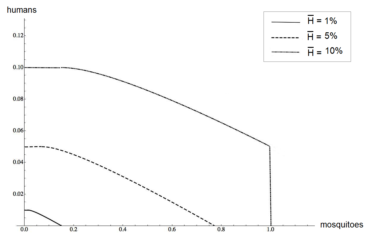
On the Figure 2, we display three viability kernels when the constraint is medium (corresponding to three values for the maximum tolerated proportion H¯¯𝐻\overline{H} of infected humans).

Refer to caption
Figure 2: Three viability kernels for the Ross-MacDonald model (1), when the constraint is medium (corresponding to three values for the maximum tolerated proportion H¯¯𝐻\overline{H} of infected humans). Parameters are adjusted to the 2013 dengue outbreak in Cali, Colombia.

The proof consists of four lemmas. In Lemma 10, we describe the solution to (31a)–(31b) (Lemma 11 provides additional information, that will be useful). Lemma 12 shows that the set

𝕍=([0,M¯]×[0,H¯]){(m,h)|M¯mM,0h(m)}𝕍0¯𝑀0¯𝐻conditional-set𝑚formulae-sequence¯𝑀𝑚subscript𝑀0𝑚\mathbb{V}=\left([0,\overline{M}]\times[0,\overline{H}]\right)\bigcup\left\{(m,h)\Big{|}\overline{M}\leq m\leq M_{\infty}\;,\enspace 0\leq h\leq\mathscr{H}(m)\right\} (34)

is a viability domain. Finally, in Lemma 13 we prove that the set 𝕍𝕍\mathbb{V}, defined in (34), is the largest viability domain within the constraint set (8), hence is the viability kernel by Theorem 3.

Lemma 10.

When the inequalities (30b) are fulfilled, there exists a function \mathscr{H}, solution to the differential equation (31a) which satisfies the initial condition (31b) and has the form (32). The function :[M¯,M][(M),H¯]:¯𝑀subscript𝑀subscript𝑀¯𝐻\mathscr{H}:[\overline{M},M_{\infty}]\to[\mathscr{H}(M_{\infty}),\overline{H}] is a strictly decreasing one-to-one mapping.

Proof.

We conduct the proof in five steps.

  1. 1.

    First, we note that

    gm(M¯,H¯,u¯)subscript𝑔𝑚¯𝑀¯𝐻¯𝑢\displaystyle g_{m}(\overline{M},\overline{H},\overline{u}) =\displaystyle= AmH¯(1M¯)u¯M¯ by (10a)subscript𝐴𝑚¯𝐻1¯𝑀¯𝑢¯𝑀 by (10a)\displaystyle A_{m}\overline{H}(1-\overline{M})-\overline{u}\overline{M}\text{ by~{}\eqref{eq:campo-control-vector_mos} }
    =\displaystyle= AmH¯(AmH¯+u¯)M¯subscript𝐴𝑚¯𝐻subscript𝐴𝑚¯𝐻¯𝑢¯𝑀\displaystyle A_{m}\overline{H}-(A_{m}\overline{H}+\overline{u})\overline{M}
    =\displaystyle= AmH¯(AmH¯+u¯)γH¯Ah(1H¯) by definition (28) of M¯subscript𝐴𝑚¯𝐻subscript𝐴𝑚¯𝐻¯𝑢𝛾¯𝐻subscript𝐴1¯𝐻 by definition (28) of ¯𝑀\displaystyle A_{m}\overline{H}-(A_{m}\overline{H}+\overline{u})\frac{\gamma\overline{H}}{A_{h}(1-\overline{H})}\text{ by definition~{}\eqref{eq:hat_mos} of~{} }\overline{M}
    =\displaystyle= H¯Ah(1H¯)[AmAh(1H¯)γ(AmH¯+u¯)]¯𝐻subscript𝐴1¯𝐻delimited-[]subscript𝐴𝑚subscript𝐴1¯𝐻𝛾subscript𝐴𝑚¯𝐻¯𝑢\displaystyle\frac{\overline{H}}{A_{h}(1-\overline{H})}[A_{m}A_{h}(1-\overline{H})-\gamma(A_{m}\overline{H}+\overline{u})]
    =\displaystyle= H¯Ah(1H¯)[AmAhγu¯(AmAh+γAm)H¯]¯𝐻subscript𝐴1¯𝐻delimited-[]subscript𝐴𝑚subscript𝐴𝛾¯𝑢subscript𝐴𝑚subscript𝐴𝛾subscript𝐴𝑚¯𝐻\displaystyle\frac{\overline{H}}{A_{h}(1-\overline{H})}[A_{m}A_{h}-\gamma\overline{u}-(A_{m}A_{h}+\gamma A_{m})\overline{H}]
    <\displaystyle< 0 by (30b).0 by (30b).\displaystyle 0\text{ by~{}\eqref{eq:cota-media_b}.}

    We easily deduce the following property, that will be useful later:

    mM¯,hH¯gm(M,H,u¯)gm(M¯,H¯,u¯)<0.formulae-sequence𝑚¯𝑀¯𝐻subscript𝑔𝑚𝑀𝐻¯𝑢subscript𝑔𝑚¯𝑀¯𝐻¯𝑢0m\geq\overline{M}\;,\enspace h\leq\overline{H}\Rightarrow g_{m}({M},{H},\overline{u})\leq g_{m}(\overline{M},\overline{H},\overline{u})<0\;. (35)
  2. 2.

    Second, we show that there is a local solution to the differential equation (31a)–(31b). Indeed, in the neighborhood of (M¯,(M¯))=(M¯,H¯)¯𝑀¯𝑀¯𝑀¯𝐻(\overline{M},\mathscr{H}(\overline{M}))=(\overline{M},\overline{H}), the coefficient gm(m,h,u¯)subscript𝑔𝑚𝑚¯𝑢g_{m}(m,h,\overline{u}) of (m)superscript𝑚\mathscr{H}^{\prime}(m) in (31a) is negative, as we just saw it in the previous item 1. Hence, in a neighborhood of M¯¯𝑀\overline{M}, we can write (31a) as

    (m)=gh(m,(m))gm(m,(m),u¯)=Ahm(1(m))γ(m)Am(m)(1m)u¯m.superscript𝑚subscript𝑔𝑚𝑚subscript𝑔𝑚𝑚𝑚¯𝑢subscript𝐴𝑚1𝑚𝛾𝑚subscript𝐴𝑚𝑚1𝑚¯𝑢𝑚\mathscr{H}^{\prime}(m)=\frac{g_{h}(m,\mathscr{H}(m))}{g_{m}(m,\mathscr{H}(m),\overline{u})}=\frac{A_{h}m(1-\mathscr{H}(m))-\gamma\mathscr{H}(m)}{A_{m}\mathscr{H}(m)(1-m)-\overline{u}m}\;. (36)

    Applying the Cauchy-Lipschitz theorem to (36)–(31b), we know that there exists a unique local C1superscript𝐶1C^{1} solution \mathscr{H} defined on an interval I𝐼I around M¯¯𝑀\overline{M}. We put

    I+=I[M¯,+[.I_{+}=I\cap[\overline{M},+\infty[\;. (37)
  3. 3.

    Third, we show that the local solution :I+:subscript𝐼\mathscr{H}:I_{+}\to\mathbb{R} is strictly decreasing in the neighborhood of M¯¯𝑀\overline{M}. For this purpose, we will study the sign of gh(m,(m))subscript𝑔𝑚𝑚g_{h}(m,\mathscr{H}(m)) for mM¯𝑚¯𝑀m\approx\overline{M}. We have that

    gh(m,(m))subscript𝑔𝑚𝑚\displaystyle g_{h}(m,\mathscr{H}(m)) =\displaystyle= gh(m,(m))gh(M¯,H¯) by (29)subscript𝑔𝑚𝑚subscript𝑔¯𝑀¯𝐻 by (29)\displaystyle g_{h}(m,\mathscr{H}(m))-g_{h}(\overline{M},\overline{H})\text{ by~{}\eqref{eq:carac_hat_mos}}
    =\displaystyle= Ahm(1(m))γ(m)AhM¯(1H¯)+γH¯subscript𝐴𝑚1𝑚𝛾𝑚subscript𝐴¯𝑀1¯𝐻𝛾¯𝐻\displaystyle A_{h}m(1-\mathscr{H}(m))-\gamma\mathscr{H}(m)-A_{h}\overline{M}(1-\overline{H})+\gamma\overline{H}
    =\displaystyle= Ah(mM¯)(1H¯)+(Ahm+γ)(H¯(m)).subscript𝐴𝑚¯𝑀1¯𝐻subscript𝐴𝑚𝛾¯𝐻𝑚\displaystyle A_{h}(m-\overline{M})(1-\overline{H})+(A_{h}m+\gamma)(\overline{H}-\mathscr{H}(m))\;.

    We have that (m)H¯=o(mM¯)𝑚¯𝐻𝑜𝑚¯𝑀\mathscr{H}(m)-\overline{H}=o(m-\overline{M}) when mM¯𝑚¯𝑀m\to\overline{M}. Indeed, the function \mathscr{H} is C1superscript𝐶1C^{1} and such that (M¯)=0superscript¯𝑀0\mathscr{H}^{\prime}(\overline{M})=0, by (36) since gh(M¯,H¯)=0subscript𝑔¯𝑀¯𝐻0g_{h}(\overline{M},\overline{H})=0 by (29). Therefore, we deduce that

    gh(m,(m))=Ah(mM¯)(1H¯)+o(mM¯).subscript𝑔𝑚𝑚subscript𝐴𝑚¯𝑀1¯𝐻𝑜𝑚¯𝑀g_{h}(m,\mathscr{H}(m))=A_{h}(m-\overline{M})(1-\overline{H})+o(m-\overline{M})\;. (38)

    Hence, when m>M¯𝑚¯𝑀m>\overline{M} and mM¯𝑚¯𝑀m\approx\overline{M}, we have that gh(m,(m))>0subscript𝑔𝑚𝑚0g_{h}(m,\mathscr{H}(m))>0. Therefore, by (36) and item 1, the function :I+:subscript𝐼\mathscr{H}:I_{+}\to\mathbb{R} is strictly decreasing in a neighborhood of M¯¯𝑀\overline{M}.

  4. 4.

    Fourth, we show that the local solution :I+:subscript𝐼\mathscr{H}:I_{+}\to\mathbb{R} is strictly decreasing. Indeed, let us suppose the contrary: there exists mI+𝑚subscript𝐼m\in I_{+}, m>M¯𝑚¯𝑀m>\overline{M}, such that (m)=0superscript𝑚0\mathscr{H}^{\prime}(m)=0. We denote by m~~𝑚\tilde{m} the smallest of such m𝑚m. By item 3, we know that (m)<0superscript𝑚0\mathscr{H}^{\prime}(m)<0 in the neighborhood of M¯¯𝑀\overline{M} (except at M¯¯𝑀\overline{M}), so that m~>M¯~𝑚¯𝑀\tilde{m}>\overline{M}. By definition of m~~𝑚\tilde{m}, we have that (m)<0superscript𝑚0\mathscr{H}^{\prime}(m)<0 for m]M¯,m~[m\in]\overline{M},\tilde{m}[. Hence, (m~)<(M¯)=H¯~𝑚¯𝑀¯𝐻\mathscr{H}(\tilde{m})<\mathscr{H}(\overline{M})=\overline{H}, so that

    gh(m~,(m~))subscript𝑔~𝑚~𝑚\displaystyle g_{h}(\tilde{m},\mathscr{H}(\tilde{m})) =\displaystyle= Ahm~(1(m~))γ(m~) by (10)subscript𝐴~𝑚1~𝑚𝛾~𝑚 by (10)\displaystyle A_{h}\tilde{m}(1-\mathscr{H}(\tilde{m}))-\gamma\mathscr{H}(\tilde{m})\text{ by~{}\eqref{eq:campo-control-vector}}
    >\displaystyle> AhM¯(1H¯)γH¯subscript𝐴¯𝑀1¯𝐻𝛾¯𝐻\displaystyle A_{h}\overline{M}(1-\overline{H})-\gamma\overline{H}
    =\displaystyle= gh(M¯,H¯)=0 by (29).subscript𝑔¯𝑀¯𝐻0 by (29).\displaystyle g_{h}(\overline{M},\overline{H})=0\text{ by~{}\eqref{eq:carac_hat_mos}.}

    As a consequence, by the differential equation (36) and item 1, we obtain that (m~)>0superscript~𝑚0\mathscr{H}^{\prime}(\tilde{m})>0. We arrive at a contradiction, since (m~)=0superscript~𝑚0\mathscr{H}^{\prime}(\tilde{m})=0 by definition of m~~𝑚\tilde{m}. Therefore, m~~𝑚\tilde{m} does not exist and the local solution :I+:subscript𝐼\mathscr{H}:I_{+}\to\mathbb{R} is strictly decreasing.

  5. 5.

    Finally, we show that the local solution :I+:subscript𝐼\mathscr{H}:I_{+}\to\mathbb{R} is such that (32) holds true. For this purpose, we consider two cases.

    • If, for every mI+𝑚subscript𝐼m\in I_{+}, 0<(m)0𝑚0<\mathscr{H}(m), we show that I+=[M¯,+[I_{+}=[\overline{M},+\infty[. Indeed, as \mathscr{H} decreases, we have mI+0<(m)(M¯)=H¯𝑚subscript𝐼0𝑚¯𝑀¯𝐻m\in I_{+}\Rightarrow 0<\mathscr{H}(m)\leq\mathscr{H}(\overline{M})=\overline{H}. Hence, we deduce that the solution (m)𝑚\mathscr{H}(m) to the equation (31a) exists over m[M¯,+[m\in[\overline{M},+\infty[. We denote M=1subscript𝑀1M_{\infty}=1.

    • If there exists an mI+𝑚subscript𝐼m\in I_{+} such that (m)=0𝑚0\mathscr{H}(m)=0, we denote by m~~𝑚\tilde{m} the smallest of such m𝑚m. We have that (m~)=0~𝑚0\mathscr{H}(\tilde{m})=0 and, since \mathscr{H} decreases, we have that (m~)=0(m)(M¯)=H¯~𝑚0𝑚¯𝑀¯𝐻\mathscr{H}(\tilde{m})=0\leq\mathscr{H}(m)\leq\mathscr{H}(\overline{M})=\overline{H} for every m[M¯,m~]𝑚¯𝑀~𝑚m\in[\overline{M},\tilde{m}].

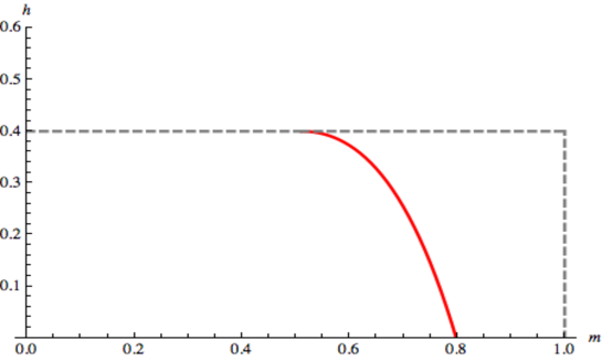
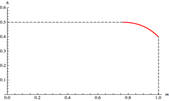
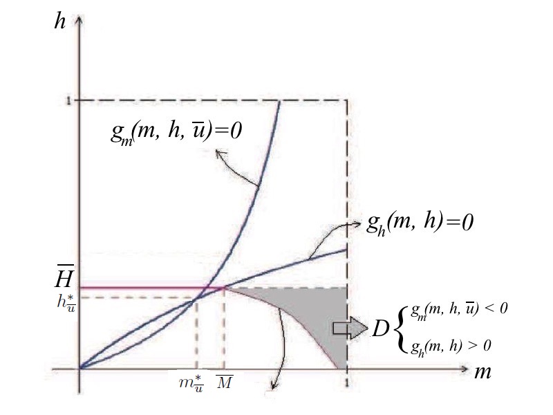
      We consider two subcases, as illustrated in Figures 3 and 4.

      • If m~<1~𝑚1\tilde{m}<1, we have that (m~)=0~𝑚0\mathscr{H}(\tilde{m})=0 and that 0(m)H¯0𝑚¯𝐻0\leq\mathscr{H}(m)\leq\overline{H} for all m[M¯,m~]𝑚¯𝑀~𝑚m\in[\overline{M},\tilde{m}]. We denote M=m~<1subscript𝑀~𝑚1M_{\infty}=\tilde{m}<1.

        Refer to caption
        Figure 3: Case M<1subscript𝑀1M_{\infty}<1. Solution graph for the differential equation (31a)–(31b), with parameters Ah=subscript𝐴absentA_{h}=0.31066, Am=subscript𝐴𝑚absentA_{m}=0.02906, γ=0.1𝛾0.1\gamma=0.1, u¯=¯𝑢absent\overline{u}=0.03733 and H¯=¯𝐻absent\overline{H}= 0.4
      • if m~1~𝑚1\tilde{m}\geq 1, we deduce that 0(m)H¯0𝑚¯𝐻0\leq\mathscr{H}(m)\leq\overline{H} for every m[M¯,1]𝑚¯𝑀1m\in[\overline{M},1]. We denote M=1subscript𝑀1M_{\infty}=1.

        Refer to caption
        Figure 4: Case M=1subscript𝑀1M_{\infty}=1. Solution graph for the differential equation (31a)–(31b), with parameters Ah=subscript𝐴absentA_{h}=0.31066, Am=subscript𝐴𝑚absentA_{m}=0.02906, γ=0.1𝛾0.1\gamma=0.1, u¯=¯𝑢absent\overline{u}=0.03733 and H¯=¯𝐻absent\overline{H}= 0.5

Hence, we conclude that the solution to the differential equation (31a), which satisfies the initial condition (31b), is unique, has the form (32) and is strictly decreasing. As (M¯)=H¯¯𝑀¯𝐻\mathscr{H}(\overline{M})=\overline{H}, the function :[M¯,M][(M),H¯]:¯𝑀subscript𝑀subscript𝑀¯𝐻\mathscr{H}:[\overline{M},M_{\infty}]\to[\mathscr{H}(M_{\infty}),\overline{H}] is a strictly decreasing one-to-one mapping. ∎

We know show that the curve generated by the solution \mathscr{H} is an orbit.

Lemma 11.

The curve

{(m,(m))m[M¯,M]}conditional-set𝑚𝑚𝑚¯𝑀subscript𝑀\{\big{(}m,\mathscr{H}(m)\big{)}\mid m\in[\overline{M},M_{\infty}]\} (39)

is an orbit of the vector field the vector (gm,gh)subscript𝑔𝑚subscript𝑔(g_{m},g_{h}), for the control u¯¯𝑢\overline{u}. Indeed, for all

m¯¯0[M¯,M] and h¯¯0=(m¯¯0)[(M),H¯],subscript¯¯𝑚0¯𝑀subscript𝑀 and subscript¯¯0subscript¯¯𝑚0subscript𝑀¯𝐻\overline{\overline{m}}_{0}\in[\overline{M},M_{\infty}]\text{ and }\overline{\overline{h}}_{0}=\mathscr{H}(\overline{\overline{m}}_{0})\in[\mathscr{H}(M_{\infty}),\overline{H}]\;, (40)

there exists T0𝑇0T\geq 0 such that the orbit of the trajectory t[0,T](m¯¯(t),h¯¯(t))𝑡0𝑇maps-to¯¯𝑚𝑡¯¯𝑡t\in[0,T]\mapsto\big{(}\overline{\overline{m}}(t),\overline{\overline{h}}(t)\big{)} — the solution to (4) when u(t)=u¯𝑢𝑡¯𝑢u(t)=\overline{u} and when the starting point is (m¯¯(0),h¯¯(0))=(m¯¯0,h¯¯0)¯¯𝑚0¯¯0subscript¯¯𝑚0subscript¯¯0\big{(}\overline{\overline{m}}(0),\overline{\overline{h}}(0)\big{)}=(\overline{\overline{m}}_{0},\overline{\overline{h}}_{0}) — is included in the curve (39). In addition,

m¯¯(T)=M¯ and h¯¯(T)=M¯.¯¯𝑚𝑇¯𝑀 and ¯¯𝑇¯𝑀\overline{\overline{m}}(T)=\overline{M}\text{ and }\overline{\overline{h}}(T)=\overline{M}\;. (41)
Proof.

When m¯¯0=M¯subscript¯¯𝑚0¯𝑀\overline{\overline{m}}_{0}=\overline{M}, then (m¯¯0)=(M¯)=H¯subscript¯¯𝑚0¯𝑀¯𝐻\mathscr{H}(\overline{\overline{m}}_{0})=\mathscr{H}(\overline{M})=\overline{H} by (31b), and the point (m¯¯0,h¯¯0)=(M¯,H¯)subscript¯¯𝑚0subscript¯¯0¯𝑀¯𝐻\big{(}\overline{\overline{m}}_{0},\overline{\overline{h}}_{0}\big{)}=(\overline{M},\overline{H}) indeed belongs to the curve (31b). Therefore T=0𝑇0T=0.

Now, we suppose that m¯¯0>M¯subscript¯¯𝑚0¯𝑀\overline{\overline{m}}_{0}>\overline{M}, so that (m¯¯0)<H¯subscript¯¯𝑚0¯𝐻\mathscr{H}(\overline{\overline{m}}_{0})<\overline{H} because \mathscr{H} is strictly decreasing by Lemma 10. We define

T=inf{t0m¯¯(t)<M¯ or h¯¯(t)>H¯},𝑇infimumconditional-set𝑡0¯¯𝑚𝑡expectation¯𝑀 or ¯¯𝑡¯𝐻T=\inf\{t\geq 0\mid\overline{\overline{m}}(t)<\overline{M}\text{ or }\overline{\overline{h}}(t)>\overline{H}\}\;, (42)

which is such that T>0𝑇0T>0, since m¯¯(0)=m¯¯0>M¯¯¯𝑚0subscript¯¯𝑚0¯𝑀\overline{\overline{m}}(0)=\overline{\overline{m}}_{0}>\overline{M} and h¯¯(0)=(m¯¯0)<H¯¯¯0subscript¯¯𝑚0¯𝐻\overline{\overline{h}}(0)=\mathscr{H}(\overline{\overline{m}}_{0})<\overline{H}.

We prove that T<+𝑇T<+\infty. Since the inequality (30b) is fulfilled by assumption, the condition (14) is satisfied, so that the endemic equilibrium point (mu¯,hu¯)subscriptsuperscript𝑚¯𝑢subscriptsuperscript¯𝑢(m^{*}_{\overline{u}},h^{*}_{\overline{u}}) in (21) exists. By definition of an equilibrium point, we have that gm(mu¯,hu¯,u¯)=0subscript𝑔𝑚subscriptsuperscript𝑚¯𝑢subscriptsuperscript¯𝑢¯𝑢0g_{m}(m^{*}_{\overline{u}},h^{*}_{\overline{u}},\overline{u})=0. Therefore, as the left hand side of inequality (30a) can be restated as hu¯<H¯subscriptsuperscript¯𝑢¯𝐻h^{*}_{\overline{u}}<\overline{H}, we deduce that mu¯<M¯subscriptsuperscript𝑚¯𝑢¯𝑀m^{*}_{\overline{u}}<\overline{M}, by (35). As seen in §2.4, the endemic equilibrium point (21) displays global asymptotic stability. Therefore, m¯¯(t)mu¯¯¯𝑚𝑡subscriptsuperscript𝑚¯𝑢\overline{\overline{m}}(t)\to m^{*}_{\overline{u}} when t+𝑡t\to+\infty. As mu¯<M¯subscriptsuperscript𝑚¯𝑢¯𝑀m^{*}_{\overline{u}}<\overline{M}, we deduce that there is a time t𝑡t such that m¯¯(t)<M¯¯¯𝑚𝑡¯𝑀\overline{\overline{m}}(t)<\overline{M}. As a consequence, T𝑇T as defined in (42) is finite: T<+𝑇T<+\infty.

We now study the trajectory t[0,T](m¯¯(t),h¯¯(t))𝑡0𝑇maps-to¯¯𝑚𝑡¯¯𝑡t\in[0,T]\mapsto\big{(}\overline{\overline{m}}(t),\overline{\overline{h}}(t)\big{)}. By definition (42) of T𝑇T, we have that

m¯¯(T)=M¯ or h¯¯(T)=M¯¯¯𝑚𝑇¯𝑀 or ¯¯𝑇¯𝑀\overline{\overline{m}}(T)=\overline{M}\text{ or }\overline{\overline{h}}(T)=\overline{M} (43a)
and that
m¯¯(t)M¯ and h¯¯(t)H¯,t[0,T].formulae-sequence¯¯𝑚𝑡¯𝑀 and ¯¯𝑡¯𝐻for-all𝑡0𝑇\overline{\overline{m}}(t)\geq\overline{M}\text{ and }\overline{\overline{h}}(t)\leq\overline{H}\;,\enspace\forall t\in[0,T]\;. (43b)

By (35) and (43b), we deduce that

dm¯¯(t)dt=gm(m¯¯(t),h¯¯(t),u¯)<0,t[0,T].formulae-sequence𝑑¯¯𝑚𝑡𝑑𝑡subscript𝑔𝑚¯¯𝑚𝑡¯¯𝑡¯𝑢0for-all𝑡0𝑇\frac{d\overline{\overline{m}}(t)}{dt}=g_{m}(\overline{\overline{m}}(t),\overline{\overline{h}}(t),\overline{u})<0\;,\enspace\forall t\in[0,T]\;.

As m¯¯0Msubscript¯¯𝑚0subscript𝑀\overline{\overline{m}}_{0}\leq M_{\infty} by (40), we deduce that m¯¯(t)m¯¯0M¯¯𝑚𝑡subscript¯¯𝑚0subscript𝑀\overline{\overline{m}}(t)\leq\overline{\overline{m}}_{0}\leq M_{\infty}, for all t[0,T]𝑡0𝑇t\in[0,T]. Together with m¯¯(t)M¯¯¯𝑚𝑡¯𝑀\overline{\overline{m}}(t)\geq\overline{M}, we obtain that m¯¯(t)[M¯,M]¯¯𝑚𝑡¯𝑀subscript𝑀\overline{\overline{m}}(t)\in[\overline{M},M_{\infty}], for all t[0,T]𝑡0𝑇t\in[0,T]. Therefore, (m¯¯(t))¯¯𝑚𝑡\mathscr{H}(\overline{\overline{m}}(t)) is well defined since :[M¯,M][(M),H¯]:¯𝑀subscript𝑀subscript𝑀¯𝐻\mathscr{H}:[\overline{M},M_{\infty}]\to[\mathscr{H}(M_{\infty}),\overline{H}] by (32). We have, for all t[0,T]𝑡0𝑇t\in[0,T],

ddt[h¯¯(t)(m¯¯(t))]=𝑑𝑑𝑡delimited-[]¯¯𝑡¯¯𝑚𝑡absent\displaystyle\frac{d}{dt}[\overline{\overline{h}}(t)-\mathscr{H}(\overline{\overline{m}}(t))]= gm(m¯¯(t),h¯¯(t),u¯)(m¯¯(t))gh(m¯¯(t),h¯¯(t))subscript𝑔𝑚¯¯𝑚𝑡¯¯𝑡¯𝑢superscript¯¯𝑚𝑡subscript𝑔¯¯𝑚𝑡¯¯𝑡\displaystyle g_{m}(\overline{\overline{m}}(t),\overline{\overline{h}}(t),\overline{u})-\mathscr{H}^{\prime}(\overline{\overline{m}}(t))g_{h}(\overline{\overline{m}}(t),\overline{\overline{h}}(t))
by (4) and (10)
=\displaystyle= 0 by (31a).0 by (31a).\displaystyle 0\text{ by~{}\eqref{eq:frontera-derecha}.}

Therefore, for all t[0,T]𝑡0𝑇t\in[0,T],

h¯¯(t)(m¯¯(t))=h¯¯(0)(m¯¯(0))=0 by (40),¯¯𝑡¯¯𝑚𝑡¯¯0¯¯𝑚00 by (40),\overline{\overline{h}}(t)-\mathscr{H}(\overline{\overline{m}}(t))=\overline{\overline{h}}(0)-\mathscr{H}(\overline{\overline{m}}(0))=0\text{ by~{}\eqref{eq:on_the_curve_frontera-derecha},} (44)

so that the trajectory t[0,T](m¯¯(t),h¯¯(t))𝑡0𝑇maps-to¯¯𝑚𝑡¯¯𝑡t\in[0,T]\mapsto\big{(}\overline{\overline{m}}(t),\overline{\overline{h}}(t)\big{)} is included in the curve (39).

As a particular case, we have that h¯¯(T)(m¯¯(T))=0¯¯𝑇¯¯𝑚𝑇0\overline{\overline{h}}(T)-\mathscr{H}(\overline{\overline{m}}(T))=0. As m¯¯(T)=M¯¯¯𝑚𝑇¯𝑀\overline{\overline{m}}(T)=\overline{M} or h¯¯(T)=M¯¯¯𝑇¯𝑀\overline{\overline{h}}(T)=\overline{M} by (43a), we conclude that

m¯¯(T)=M¯ and h¯¯(T)=M¯,¯¯𝑚𝑇¯𝑀 and ¯¯𝑇¯𝑀\overline{\overline{m}}(T)=\overline{M}\text{ and }\overline{\overline{h}}(T)=\overline{M}\;,

since the function :[M¯,M][(M),H¯]:¯𝑀subscript𝑀subscript𝑀¯𝐻\mathscr{H}:[\overline{M},M_{\infty}]\to[\mathscr{H}(M_{\infty}),\overline{H}] is a strictly decreasing one-to-one mapping. We have proven (41). ∎

Lemma 12.

When the inequalities (30b) are fulfilled, the set 𝕍𝕍\mathbb{V}, defined in (34), is a viability domain for the system (4)–(5).

Proof.

Let the Hamiltonian \mathscr{L} be defined, for every vector (nm,nh)subscript𝑛𝑚subscript𝑛(n_{m},n_{h}), every state (m,h)𝑚(m,h) and control u𝑢u, by

(m,h,nm,nh,u)=gm(m,h,u)nm+gh(m,h)nh.𝑚subscript𝑛𝑚subscript𝑛𝑢subscript𝑔𝑚𝑚𝑢subscript𝑛𝑚subscript𝑔𝑚subscript𝑛\mathscr{L}(m,h,n_{m},n_{h},u)=g_{m}(m,h,u)n_{m}+g_{h}(m,h)n_{h}\;. (45)

The Hamiltonian is the scalar product between the vectors (gm,gh)subscript𝑔𝑚subscript𝑔(g_{m},g_{h}) and (nm,nh)subscript𝑛𝑚subscript𝑛(n_{m},n_{h}).

We will check that, for any given point along the piecewise-smooth frontier of the set 𝕍𝕍\mathbb{V}, defined in (34), there is at least one control u[u¯,u¯]𝑢¯𝑢¯𝑢u\in[\underline{u},\overline{u}] such that the value (45) of the Hamiltonian is lower than or equal to zero when (nm,nh)subscript𝑛𝑚subscript𝑛(n_{m},n_{h}) is a normal outward-pointing vector (with respect to the set 𝕍𝕍\mathbb{V}). For kink points between two smooth parts, we will do the same but with the cone generated by two normal outward-pointing vectors, corresponding to each of the smooth parts.

We will divide the frontier of the set 𝕍𝕍\mathbb{V}, defined in (34), in five or seven parts (see Figures 3 and 4) as follows.

  1. (a)

    On the horizontal segment {(m,0)|0<m<M}conditional-set𝑚00𝑚subscript𝑀\{(m,0)|0<m<M_{\infty}\}, on the vertical segment {(0,h)|0<h<H¯}conditional-set00¯𝐻\{(0,h)|0<h<\overline{H}\} and at the points (0,0)00(0,0) and (0,H¯)0¯𝐻(0,\overline{H}), all vectors (gm,gh)subscript𝑔𝑚subscript𝑔(g_{m},g_{h}) point towards the inside of the set 𝕍𝕍\mathbb{V}, defined in (34). Indeed, it suffices to copy the proof of Proposition 8.

  2. (b)

    Along the segment {(m,H¯)|0<m<M¯}conditional-set𝑚¯𝐻0𝑚¯𝑀\{(m,\overline{H})|0<m<\overline{M}\}, a normal outward-pointing vector is

    (nmnh)=(01).subscript𝑛𝑚subscript𝑛01\left(\begin{array}[]{c}n_{m}\\ n_{h}\end{array}\right)=\left(\begin{array}[]{c}0\\ 1\end{array}\right)\;.

    Therefore, for any control u[u¯,u¯]𝑢¯𝑢¯𝑢u\in[\underline{u},\overline{u}], the value (45) of the Hamiltonian is

    (m,H¯,nm,nh,u)=gh(m,H¯)×1<0,𝑚¯𝐻subscript𝑛𝑚subscript𝑛𝑢subscript𝑔𝑚¯𝐻10\displaystyle\mathscr{L}(m,\overline{H},n_{m},n_{h},u)=g_{h}(m,\overline{H})\times 1<0\;,

    by (29) and because m<M¯𝑚¯𝑀m<\overline{M}.

  3. (c)

    Along the curve {(m,(m))|M¯<m<M}conditional-set𝑚𝑚¯𝑀𝑚subscript𝑀\{(m,\mathscr{H}(m))|\overline{M}<m<M_{\infty}\}, a normal outward-pointing vector is

    (nmnh)=((m)1).subscript𝑛𝑚subscript𝑛superscript𝑚1\left(\begin{array}[]{c}n_{m}\\ n_{h}\end{array}\right)=\left(\begin{array}[]{c}-\mathscr{H}^{\prime}(m)\\ 1\end{array}\right)\;.

    Therefore, for the control u¯¯𝑢\overline{u}, the value (45) of the Hamiltonian is

    (m,H¯,nm,nh,u¯)=gm(m,(m),u¯)(m)+gh(m,(m))×1=0,𝑚¯𝐻subscript𝑛𝑚subscript𝑛¯𝑢subscript𝑔𝑚𝑚𝑚¯𝑢superscript𝑚subscript𝑔𝑚𝑚10\mathscr{L}(m,\overline{H},n_{m},n_{h},\overline{u})=-g_{m}(m,\mathscr{H}(m),\overline{u})\mathscr{H}^{\prime}(m)+g_{h}(m,\mathscr{H}(m))\times 1=0\;,

    because the function \mathscr{H} is the solution to the differential equation (31a).

  4. (d)

    The point (M¯,H¯)¯𝑀¯𝐻(\overline{M},\overline{H}) is a kink, to which is attached a cone of normal vectors generated by the two following normal outward-pointing vectors.

    • A normal outward-pointing vector to the horizontal segment {(m,H¯)|0mM¯}conditional-set𝑚¯𝐻0𝑚¯𝑀\{(m,\overline{H})|0\leq m\leq\overline{M}\} at the kink point (M¯,H¯)¯𝑀¯𝐻(\overline{M},\overline{H}) is

      (nmnh)=(01).subscript𝑛𝑚subscript𝑛01\left(\begin{array}[]{c}n_{m}\\ n_{h}\end{array}\right)=\left(\begin{array}[]{c}0\\ 1\end{array}\right)\;.

      Therefore, for any control u[u¯,u¯]𝑢¯𝑢¯𝑢u\in[\underline{u},\overline{u}], the value (45) of the Hamiltonian is

      (M¯,H¯,nm,nh,u)=gh(M¯,H¯)×1=0 by (29).¯𝑀¯𝐻subscript𝑛𝑚subscript𝑛𝑢subscript𝑔¯𝑀¯𝐻10 by (29).\mathscr{L}(\overline{M},\overline{H},n_{m},n_{h},u)=g_{h}(\overline{M},\overline{H})\times 1=0\text{ by~{}\eqref{eq:carac_hat_mos}.}
    • A normal outward-pointing vector to the curve {(m,(m))|M¯mM}conditional-set𝑚𝑚¯𝑀𝑚subscript𝑀\{(m,\mathscr{H}(m))|\overline{M}\leq m\leq M_{\infty}\} at the kink point (M¯,H¯)¯𝑀¯𝐻(\overline{M},\overline{H}) is

      (nmnh)=((M)1)=(01) by (36) and (29).subscript𝑛𝑚subscript𝑛superscript𝑀101 by (36) and (29).\left(\begin{array}[]{c}n_{m}\\ n_{h}\end{array}\right)=\left(\begin{array}[]{c}-\mathscr{H}^{\prime}({M})\\ 1\end{array}\right)=\left(\begin{array}[]{c}0\\ 1\end{array}\right)\text{ by~{}\eqref{eq:frontera-derecha-equivalente} and~{}\eqref{eq:carac_hat_mos}.}

      Therefore, for any control u[u¯,u¯]𝑢¯𝑢¯𝑢u\in[\underline{u},\overline{u}], the value (45) of the Hamiltonian is

      (M¯,H¯,nm,nh,u)=gh(M¯,H¯)×1=0 by (29).¯𝑀¯𝐻subscript𝑛𝑚subscript𝑛𝑢subscript𝑔¯𝑀¯𝐻10 by (29).\mathscr{L}(\overline{M},\overline{H},n_{m},n_{h},u)=g_{h}(\overline{M},\overline{H})\times 1=0\text{ by~{}\eqref{eq:carac_hat_mos}.}

    We conclude that, for any control u[u¯,u¯]𝑢¯𝑢¯𝑢u\in[\underline{u},\overline{u}], the value (45) of the Hamiltonian is zero for any combination of the two normal outward-pointing vectors above. As a consequence, all vectors (gm,gh)subscript𝑔𝑚subscript𝑔(g_{m},g_{h}) point towards the inside of the set 𝕍𝕍\mathbb{V}, defined in (34), at the kink point (M¯,H¯)¯𝑀¯𝐻(\overline{M},\overline{H}).

  5. (e)

    When M<1subscript𝑀1M_{\infty}<1 in (32) (see Figure 3), there only remains to consider the kink point (M,0)subscript𝑀0(M_{\infty},0).

    • A normal outward-pointing vector to the horizontal segment {(m,0)|0mM}conditional-set𝑚00𝑚subscript𝑀\{(m,0)|0\leq m\leq M_{\infty}\} at the kink point (M,0)subscript𝑀0(M_{\infty},0) is

      (nmnh)=(10).subscript𝑛𝑚subscript𝑛10\left(\begin{array}[]{c}n_{m}\\ n_{h}\end{array}\right)=\left(\begin{array}[]{c}1\\ 0\end{array}\right)\;.

      Therefore, for any control u[u¯,u¯]𝑢¯𝑢¯𝑢u\in[\underline{u},\overline{u}], the value (45) of the Hamiltonian is

      (M,0,nm,nh,u)=gm(M,0,u)×1=uMu¯M0.subscript𝑀0subscript𝑛𝑚subscript𝑛𝑢subscript𝑔𝑚subscript𝑀0𝑢1𝑢subscript𝑀¯𝑢subscript𝑀0\mathscr{L}(M_{\infty},0,n_{m},n_{h},u)=g_{m}(M_{\infty},0,u)\times 1=-uM_{\infty}\leq-\underline{u}M_{\infty}\leq 0\;.
    • A normal outward-pointing vector to the curve {(m,(m))|M¯mM}conditional-set𝑚𝑚¯𝑀𝑚subscript𝑀\{(m,\mathscr{H}(m))|\overline{M}\leq m\leq M_{\infty}\} at the kink point (M,0)subscript𝑀0(M_{\infty},0) is

      (nmnh)=((M)1).subscript𝑛𝑚subscript𝑛superscriptsubscript𝑀1\left(\begin{array}[]{c}n_{m}\\ n_{h}\end{array}\right)=\left(\begin{array}[]{c}-\mathscr{H}^{\prime}(M_{\infty})\\ 1\end{array}\right)\;.

      Therefore, for the control u¯¯𝑢\overline{u}, the value (45) of the Hamiltonian is

      (M,0,nm,nh,u¯)subscript𝑀0subscript𝑛𝑚subscript𝑛¯𝑢\displaystyle\mathscr{L}(M_{\infty},0,n_{m},n_{h},\overline{u}) =\displaystyle= gm(M,0,u¯)(M)+gh(M,0)×1subscript𝑔𝑚subscript𝑀0¯𝑢superscriptsubscript𝑀subscript𝑔subscript𝑀01\displaystyle-g_{m}(M_{\infty},0,\overline{u})\mathscr{H}^{\prime}(M_{\infty})+g_{h}(M_{\infty},0)\times 1
      =\displaystyle= 0 by (31a).0 by (31a).\displaystyle 0\text{ by~{}\eqref{eq:frontera-derecha}.}

    We conclude that, for the control u¯¯𝑢\overline{u}, the value (45) of the Hamiltonian is zero for any combination of the two normal outward-pointing vectors above. As a consequence, the vector (gm,gh)subscript𝑔𝑚subscript𝑔(g_{m},g_{h}), for the control u¯¯𝑢\overline{u}, points towards the inside of the set 𝕍𝕍\mathbb{V}, defined in (34), at the kink point (M,0)subscript𝑀0(M_{\infty},0).

  6. (f)

    When M=1subscript𝑀1M_{\infty}=1 in (32) (see Figure 4), we have to consider the vertical segment {(1,h)|0h<(1)}conditional-set101\{(1,h)|0\leq h<\mathscr{H}(1)\}. A normal outward-pointing vector to the vertical segment {(1,h)|0h<(1)}conditional-set101\{(1,h)|0\leq h<\mathscr{H}(1)\} has the form

    (nmnh)=(10).subscript𝑛𝑚subscript𝑛10\left(\begin{array}[]{c}n_{m}\\ n_{h}\end{array}\right)=\left(\begin{array}[]{c}1\\ 0\end{array}\right)\;.

    Therefore, for any control u[u¯,u¯]𝑢¯𝑢¯𝑢u\in[\underline{u},\overline{u}], the value (45) of the Hamiltonian is

    (1,h,nm,nh,u)=gm(1,h,u)×1=uu¯0.1subscript𝑛𝑚subscript𝑛𝑢subscript𝑔𝑚1𝑢1𝑢¯𝑢0\mathscr{L}(1,h,n_{m},n_{h},u)=g_{m}(1,h,u)\times 1=-u\leq-\underline{u}\leq 0\;.

    As a consequence, all vectors (gm,gh)subscript𝑔𝑚subscript𝑔(g_{m},g_{h}) point towards the inside of the set 𝕍𝕍\mathbb{V}, defined in (34), along the vertical segment {(1,h)|0h<(1)}conditional-set101\{(1,h)|0\leq h<\mathscr{H}(1)\}.

  7. (g)

    When M=1subscript𝑀1M_{\infty}=1 in (32) (see Figure 4), there remains to consider the kink point (1,(1))11(1,\mathscr{H}(1)).

    • A normal outward-pointing vector to the vertical segment {(1,h)|0h(1)}conditional-set101\{(1,h)|0\leq h\leq\mathscr{H}(1)\} at the kink point (1,(1))11(1,\mathscr{H}(1)) is

      (nmnh)=(10).subscript𝑛𝑚subscript𝑛10\left(\begin{array}[]{c}n_{m}\\ n_{h}\end{array}\right)=\left(\begin{array}[]{c}1\\ 0\end{array}\right)\;.

      Therefore, for any control u[u¯,u¯]𝑢¯𝑢¯𝑢u\in[\underline{u},\overline{u}], the value (45) of the Hamiltonian is

      (1,(1),nm,nh,u)=gm(1,(1),u)×1=uu¯<0.11subscript𝑛𝑚subscript𝑛𝑢subscript𝑔𝑚11𝑢1𝑢¯𝑢0\mathscr{L}(1,\mathscr{H}(1),n_{m},n_{h},u)=g_{m}(1,\mathscr{H}(1),u)\times 1=-u\leq-\underline{u}<0\;.
    • A normal outward-pointing vector to the curve {(m,(m))|M¯<m<M}conditional-set𝑚𝑚¯𝑀𝑚subscript𝑀\{(m,\mathscr{H}(m))|\overline{M}<m<M_{\infty}\} at the kink point (1,(1))11(1,\mathscr{H}(1)) is

      (nmnh)=((1)1).subscript𝑛𝑚subscript𝑛superscript11\left(\begin{array}[]{c}n_{m}\\ n_{h}\end{array}\right)=\left(\begin{array}[]{c}-\mathscr{H}^{\prime}(1)\\ 1\end{array}\right)\;.

      Therefore, for the control u¯¯𝑢\overline{u}, the value (45) of the Hamiltonian is

      (1,(1),nm,nh,u¯)11subscript𝑛𝑚subscript𝑛¯𝑢\displaystyle\mathscr{L}(1,\mathscr{H}(1),n_{m},n_{h},\overline{u}) =\displaystyle= gm(1,(1),u¯)(1)+gh(1,(1))×1subscript𝑔𝑚11¯𝑢superscript1subscript𝑔111\displaystyle-g_{m}(1,\mathscr{H}(1),\overline{u})\mathscr{H}^{\prime}(1)+g_{h}(1,\mathscr{H}(1))\times 1
      =\displaystyle= 0 by (31a).0 by (31a).\displaystyle 0\text{ by~{}\eqref{eq:frontera-derecha}.}

    We conclude that, for the control u¯¯𝑢\overline{u}, the value (45) of the Hamiltonian is zero for any combination of the two normal outward-pointing vectors above. As a consequence, the vector (gm,gh)subscript𝑔𝑚subscript𝑔(g_{m},g_{h}), for the control u¯¯𝑢\overline{u}, points towards the inside of the set 𝕍𝕍\mathbb{V}, defined in (34), at the kink point (1,(1))11(1,\mathscr{H}(1)).

From Proposition 5, we can conclude that 𝕍𝕍\mathbb{V}, defined in (34), is a viability domain. ∎

Lemma 13.

When the inequalities (30b) are fulfilled, the set 𝕍𝕍\mathbb{V}, defined in (34), is the largest viability domain for the system (4), within the constraint set (8).

Refer to caption
Figure 5: The shaded portion of the graph corresponds to the complement of the viability kernel 𝕍(H¯)𝕍¯𝐻\mathbb{V}(\overline{H}) with respect to the constraint set 𝕍0(H¯)superscript𝕍0¯𝐻\mathbb{V}^{0}(\overline{H}), when M<1subscript𝑀1M_{\infty}<1
Proof.

We prove that, for any control trajectory u()𝑢u(\cdot) as in (5), the trajectory t(m(t),h(t))maps-to𝑡𝑚𝑡𝑡t\mapsto\big{(}{m}(t),{h}(t)\big{)} solution of (4) and that starts from a point

(m(0),h(0))=(m0,h0)𝕍0(H¯)\𝕍𝑚00subscript𝑚0subscript0\superscript𝕍0¯𝐻𝕍\big{(}{m}(0),{h}(0)\big{)}=(m_{0},h_{0})\in\mathbb{V}^{0}(\overline{H})\backslash\mathbb{V} (46)

does not satisfy the constraint (6) for at least one t>0𝑡0t>0. In Figure 5, the set 𝕍0(H¯)\𝕍\superscript𝕍0¯𝐻𝕍\mathbb{V}^{0}(\overline{H})\backslash\mathbb{V} is represented by the shaded part (in the case when M<1subscript𝑀1M_{\infty}<1).

First, we examine the point (m0,h0)𝕍0(H¯)\𝕍subscript𝑚0subscript0\superscript𝕍0¯𝐻𝕍(m_{0},h_{0})\in\mathbb{V}^{0}(\overline{H})\backslash\mathbb{V}. On the one hand, as (m0,h0)𝕍0(H¯)subscript𝑚0subscript0superscript𝕍0¯𝐻(m_{0},h_{0})\in\mathbb{V}^{0}(\overline{H}), we have that 0h0H¯0subscript0¯𝐻0\leq h_{0}\leq\overline{H}. On the other hand, since (m0,h0)𝕍subscript𝑚0subscript0𝕍(m_{0},h_{0})\notin\mathbb{V}, where the set 𝕍𝕍\mathbb{V} is defined in (34), we deduce from Lemma 10, and especially from (32), that

(m0,h0)𝕍0(H¯)\𝕍subscript𝑚0subscript0\superscript𝕍0¯𝐻𝕍\displaystyle(m_{0},h_{0})\in\mathbb{V}^{0}(\overline{H})\backslash\mathbb{V} M¯<m01,0h0H¯\displaystyle\iff\overline{M}<m_{0}\leq 1\;,\enspace 0\leq h_{0}\leq\overline{H} (47)
and {either m0>M,or m0M and (m0)<h0.and caseseither subscript𝑚0subscript𝑀or subscript𝑚0subscript𝑀 and subscript𝑚0subscript0\displaystyle\text{ and }\begin{cases}\text{either \quad}&m_{0}>M_{\infty}\;,\\ \text{or \quad}&m_{0}\leq M_{\infty}\text{ and }\mathscr{H}(m_{0})<h_{0}\;.\end{cases}

Notice that, if h0=H¯subscript0¯𝐻h_{0}=\overline{H}, then

dh(t)dt|t=0=\displaystyle\frac{d{h}(t)}{dt}_{|t=0}= gh(m0,H¯) by (4) and (10)subscript𝑔subscript𝑚0¯𝐻 by (4) and (10)\displaystyle g_{h}({m}_{0},\overline{H})\text{ by~{}\eqref{eq:model-control-vector} and \eqref{eq:campo-control-vector} }
>\displaystyle> gh(M¯,H¯) by (10) and M¯<m0subscript𝑔¯𝑀¯𝐻 by (10) and ¯𝑀subscript𝑚0\displaystyle g_{h}(\overline{M},\overline{H})\text{ by~{}\eqref{eq:campo-control-vector} and }\overline{M}<m_{0}
=\displaystyle= 0 by (29).0 by (29).\displaystyle 0\text{ by~{}\eqref{eq:carac_hat_mos}.}

Therefore, h(t)>H¯𝑡¯𝐻{h}(t)>\overline{H}, for t>0𝑡0t>0 small enough. As a consequence, we will concentrate on the case h0<H¯subscript0¯𝐻h_{0}<\overline{H}.

Second, we show that there exists a point (m¯¯0,h¯¯0)subscript¯¯𝑚0subscript¯¯0(\overline{\overline{m}}_{0},\overline{\overline{h}}_{0}) such that

m¯¯0<m0 and m¯¯0[M¯,M] and h¯¯0=h0=(m¯¯0)H¯.subscript¯¯𝑚0subscript𝑚0 and subscript¯¯𝑚0¯𝑀subscript𝑀 and subscript¯¯0subscript0subscript¯¯𝑚0¯𝐻\overline{\overline{m}}_{0}<{m}_{0}\text{ and }\overline{\overline{m}}_{0}\in[\overline{M},M_{\infty}]\text{ and }\overline{\overline{h}}_{0}=h_{0}=\mathscr{H}(\overline{\overline{m}}_{0})\leq\overline{H}\;. (48)

Of course, we take h¯¯0=h0subscript¯¯0subscript0\overline{\overline{h}}_{0}=h_{0}. To prove the existence of m¯¯0[M¯,M]subscript¯¯𝑚0¯𝑀subscript𝑀\overline{\overline{m}}_{0}\in[\overline{M},M_{\infty}], it suffices to show that h0[(M),H¯]subscript0subscript𝑀¯𝐻h_{0}\in[\mathscr{H}(M_{\infty}),\overline{H}]. Indeed, we know from Lemma 10, and especially (32) that the function :[M¯,M][(M),H¯]:¯𝑀subscript𝑀subscript𝑀¯𝐻\mathscr{H}:[\overline{M},M_{\infty}]\to[\mathscr{H}(M_{\infty}),\overline{H}] is C1superscript𝐶1C^{1} and strictly decreasing. Now, from (47), we deduce that

  • if M=1subscript𝑀1M_{\infty}=1, then m0M=1subscript𝑚0subscript𝑀1m_{0}\leq M_{\infty}=1 and (m0)<h0H¯subscript𝑚0subscript0¯𝐻\mathscr{H}(m_{0})<h_{0}\leq\overline{H}; as the function \mathscr{H} is strictly decreasing, we conclude that (M)(m0)<h0H¯subscript𝑀subscript𝑚0subscript0¯𝐻\mathscr{H}(M_{\infty})\leq\mathscr{H}(m_{0})<h_{0}\leq\overline{H}, hence that h0[(M),H¯]subscript0subscript𝑀¯𝐻h_{0}\in[\mathscr{H}(M_{\infty}),\overline{H}];

  • if M<1subscript𝑀1M_{\infty}<1, then (M)=0subscript𝑀0\mathscr{H}(M_{\infty})=0 by (32); as 0h0H¯0subscript0¯𝐻0\leq h_{0}\leq\overline{H}, we conclude that 0=(M)<h0H¯0subscript𝑀subscript0¯𝐻0=\mathscr{H}(M_{\infty})<h_{0}\leq\overline{H}, hence that h0[(M),H¯]subscript0subscript𝑀¯𝐻h_{0}\in[\mathscr{H}(M_{\infty}),\overline{H}].

Notice in passing that, as the function \mathscr{H} is strictly decreasing, we have that

m¯¯0=M¯h¯¯0=h0=H¯.iffsubscript¯¯𝑚0¯𝑀subscript¯¯0subscript0¯𝐻\overline{\overline{m}}_{0}=\overline{M}\iff\overline{\overline{h}}_{0}=h_{0}=\overline{H}\;. (49)

We have proved that m¯¯0subscript¯¯𝑚0\overline{\overline{m}}_{0} exists and that m¯¯0[M¯,M]subscript¯¯𝑚0¯𝑀subscript𝑀\overline{\overline{m}}_{0}\in[\overline{M},M_{\infty}]. There remains to show that m¯¯0<m0subscript¯¯𝑚0subscript𝑚0\overline{\overline{m}}_{0}<{m}_{0}. Now, from m¯¯0[M¯,M]subscript¯¯𝑚0¯𝑀subscript𝑀\overline{\overline{m}}_{0}\in[\overline{M},M_{\infty}] and h¯¯0=h0=(m¯¯0)subscript¯¯0subscript0subscript¯¯𝑚0\overline{\overline{h}}_{0}=h_{0}=\mathscr{H}(\overline{\overline{m}}_{0}), we deduce that (m¯¯0,h¯¯0)=(m¯¯0,h0)𝕍subscript¯¯𝑚0subscript¯¯0subscript¯¯𝑚0subscript0𝕍(\overline{\overline{m}}_{0},\overline{\overline{h}}_{0})=(\overline{\overline{m}}_{0},{h}_{0})\in\mathbb{V}, defined in (34). By definition (34) of 𝕍𝕍\mathbb{V}, using the property that the function \mathscr{H} is strictly decreasing, we have that

(m¯¯0,h¯¯0)=(m¯¯0,h0)𝕍(m,h0)𝕍,mm¯¯0.formulae-sequencesubscript¯¯𝑚0subscript¯¯0subscript¯¯𝑚0subscript0𝕍𝑚subscript0𝕍for-all𝑚subscript¯¯𝑚0(\overline{\overline{m}}_{0},\overline{\overline{h}}_{0})=(\overline{\overline{m}}_{0},{h}_{0})\in\mathbb{V}\Rightarrow({m},{h}_{0})\in\mathbb{V}\;,\enspace\forall{m}\leq\overline{\overline{m}}_{0}\;.

As (m0,h0)𝕍subscript𝑚0subscript0𝕍({m}_{0},{h}_{0})\not\in\mathbb{V} by assumption (46), we conclude that m¯¯0<m0subscript¯¯𝑚0subscript𝑚0\overline{\overline{m}}_{0}<{m}_{0}.

From now on, we suppose that h0<H¯subscript0¯𝐻h_{0}<\overline{H}, so that, summing up the properties shown above, the point (m¯¯0,h¯¯0)subscript¯¯𝑚0subscript¯¯0(\overline{\overline{m}}_{0},\overline{\overline{h}}_{0}) is such that

m¯¯0<m0 and m¯¯0]M¯,M] and h¯¯0=h0=(m¯¯0)<H¯.\overline{\overline{m}}_{0}<{m}_{0}\text{ and }\overline{\overline{m}}_{0}\in]\overline{M},M_{\infty}]\text{ and }\overline{\overline{h}}_{0}=h_{0}=\mathscr{H}(\overline{\overline{m}}_{0})<\overline{H}\;. (50)

Now, in addition to the trajectory t(m(t),h(t))maps-to𝑡𝑚𝑡𝑡t\mapsto\big{(}{m}(t),{h}(t)\big{)} that is the solution to (4) for the control trajectory u()𝑢u(\cdot) when (m(0),h(0))=(m0,h0)𝑚00subscript𝑚0subscript0\big{(}{m}(0),{h}(0)\big{)}=({m}_{0},{h}_{0}), we study the trajectories

  • t(m¯¯(t),h¯¯(t))maps-to𝑡¯¯𝑚𝑡¯¯𝑡t\mapsto\big{(}\overline{\overline{m}}(t),\overline{\overline{h}}(t)\big{)}, the solution to (4) when u(t)=u¯𝑢𝑡¯𝑢u(t)=\overline{u} and when the starting point is (m¯¯(0),h¯¯(0))=(m¯¯0,h¯¯0)=(m¯¯0,h0)¯¯𝑚0¯¯0subscript¯¯𝑚0subscript¯¯0subscript¯¯𝑚0subscript0\big{(}\overline{\overline{m}}(0),\overline{\overline{h}}(0)\big{)}=(\overline{\overline{m}}_{0},\overline{\overline{h}}_{0})=(\overline{\overline{m}}_{0},{h}_{0}) as in (50), that is, on the right of the frontier of 𝕍𝕍\mathbb{V} (the bottom frontier of the shaded part in Figure 5);

  • t(m¯(t),h¯(t))maps-to𝑡¯𝑚𝑡¯𝑡t\mapsto\big{(}\overline{m}(t),\overline{h}(t)\big{)}, the solution to (4) when u(t)=u¯𝑢𝑡¯𝑢u(t)=\overline{u} and when the starting point is (m¯(0),h¯(0))=(m0,h0)¯𝑚0¯0subscript𝑚0subscript0\big{(}\overline{m}(0),\overline{h}(0)\big{)}=({m}_{0},{h}_{0}).

We have the following inequalities between initial conditions:

(m¯¯(0),h¯¯(0))=(m¯¯0,h¯¯0)(m0,h0)=(m(0),h(0))=(m¯(0),h¯(0)).¯¯𝑚0¯¯0subscript¯¯𝑚0subscript¯¯0subscript𝑚0subscript0𝑚00¯𝑚0¯0\big{(}\overline{\overline{m}}(0),\overline{\overline{h}}(0)\big{)}=(\overline{\overline{m}}_{0},\overline{\overline{h}}_{0})\leq({m}_{0},{h}_{0})=\big{(}{m}(0),{h}(0)\big{)}=\big{(}\overline{m}(0),\overline{h}(0)\big{)}\;.

By Proposition 6, we deduce that

(m¯¯(t),h¯¯(t))(m¯(t),h¯(t))(m(t),h(t)),t0.formulae-sequence¯¯𝑚𝑡¯¯𝑡¯𝑚𝑡¯𝑡𝑚𝑡𝑡for-all𝑡0\big{(}\overline{\overline{m}}(t),\overline{\overline{h}}(t)\big{)}\leq\big{(}\overline{m}(t),\overline{h}(t)\big{)}\leq\big{(}{m}(t),{h}(t)\big{)}\;,\enspace\forall t\geq 0\;.

By Lemma 11, we obtain in particular that there exists T>0𝑇0T>0 such that

H¯=h¯¯(T)h¯(T)h(T).¯𝐻¯¯𝑇¯𝑇𝑇\overline{H}=\overline{\overline{h}}(T)\leq\overline{h}(T)\leq{h}(T)\;.

Here, T>0𝑇0T>0 because (as can be seen in the proof of Lemma 11),

m¯¯(0)=m¯¯0>M¯ and h¯¯(0)=h¯¯0<H¯.¯¯𝑚0subscript¯¯𝑚0¯𝑀 and ¯¯0subscript¯¯0¯𝐻\overline{\overline{m}}(0)=\overline{\overline{m}}_{0}>\overline{M}\text{ and }\overline{\overline{h}}(0)=\overline{\overline{h}}_{0}<\overline{H}\;.

We prove that h¯¯(T)<h¯(T)¯¯𝑇¯𝑇\overline{\overline{h}}(T)<\overline{h}(T).

Suppose, by contradiction, that h¯¯(T)=h¯(T)¯¯𝑇¯𝑇\overline{\overline{h}}(T)=\overline{h}(T). Therefore, the function
t0h¯(t)h¯¯(t)𝑡0maps-to¯𝑡¯¯𝑡t\geq 0\mapsto\overline{h}(t)-\overline{\overline{h}}(t) is nonnegative with a minimum at T>0𝑇0T>0, so that

dh¯(t)dt|t=Tdh¯¯(t)dt|t=T=0.\frac{d\overline{h}(t)}{dt}_{|t=T}-\frac{d\overline{\overline{h}}(t)}{dt}_{|t=T}=0\;.

From (4), we deduce that

Ahm¯(T)(1h¯(T))γh¯(T)=Ahm¯¯(T)(1h¯¯(T))γh¯¯(T).subscript𝐴¯𝑚𝑇1¯𝑇𝛾¯𝑇subscript𝐴¯¯𝑚𝑇1¯¯𝑇𝛾¯¯𝑇A_{h}\overline{m}(T)(1-\overline{h}(T))-\gamma\overline{h}(T)=A_{h}\overline{\overline{m}}(T)(1-\overline{\overline{h}}(T))-\gamma\overline{\overline{h}}(T)\;.

As h¯¯(T)=h¯(T)<1¯¯𝑇¯𝑇1\overline{\overline{h}}(T)=\overline{h}(T)<1, we obtain that m¯(T)=m¯¯(T)¯𝑚𝑇¯¯𝑚𝑇\overline{m}(T)=\overline{\overline{m}}(T). Therefore, we have

(m¯¯(T),h¯¯(T))=(m¯(T),h¯(T)).¯¯𝑚𝑇¯¯𝑇¯𝑚𝑇¯𝑇\big{(}\overline{\overline{m}}(T),\overline{\overline{h}}(T)\big{)}=\big{(}\overline{m}(T),\overline{h}(T)\big{)}\;.

This is impossible because the two trajectories t(m¯¯(t),h¯¯(t))maps-to𝑡¯¯𝑚𝑡¯¯𝑡t\mapsto\big{(}\overline{\overline{m}}(t),\overline{\overline{h}}(t)\big{)}, and t(m¯(t),h¯(t))maps-to𝑡¯𝑚𝑡¯𝑡t\mapsto\big{(}\overline{m}(t),\overline{h}(t)\big{)} are generated by the same vector fields, so that they must be equal. However, we have m¯¯(0)=m¯¯0<m0=m¯(0)¯¯𝑚0subscript¯¯𝑚0subscript𝑚0¯𝑚0\overline{\overline{m}}(0)=\overline{\overline{m}}_{0}<{m}_{0}=\overline{m}(0).

To conclude, we have proven that, for any control trajectory u()𝑢u(\cdot) as in (5), the state trajectory starting from any point of the set 𝕍0(H¯)\𝕍\superscript𝕍0¯𝐻𝕍\mathbb{V}^{0}(\overline{H})\backslash\mathbb{V} does not satisfy the constraint (6) for a time T<+𝑇T<+\infty. ∎

3.4 Epidemiological interpretation

The following theorem summarizes the description of the viability kernel depending on whether the upper limit H¯¯𝐻\overline{H} for the proportion of infected humans in (6) is low, high or medium.

Theorem 14.

The viability kernel 𝕍(H¯)𝕍¯𝐻\mathbb{V}(\overline{H}) in (7) is as follows.

L)

High constraint, that is, a low threshold of infected humans. If

H¯<Ahγu¯/AmAh+γ,¯𝐻subscript𝐴𝛾¯𝑢subscript𝐴𝑚subscript𝐴𝛾\overline{H}<\frac{A_{h}-\gamma\overline{u}/A_{m}}{A_{h}+\gamma}\;,\enspace (51)

the viability kernel consists only of the origin:

𝕍(H¯)={(0,0)}.𝕍¯𝐻00\mathbb{V}(\overline{H})=\{(0,0)\}\;. (52)
H)

Weak constraint, that is, a high threshold of infected humans. If

AhAh+γ<H¯,subscript𝐴subscript𝐴𝛾¯𝐻\frac{A_{h}}{A_{h}+\gamma}<\overline{H}\;, (53)

the viability kernel 𝕍(H¯)𝕍¯𝐻\mathbb{V}(\overline{H}) is the whole constraint set, that is,

𝕍(H¯)=𝕍0(H¯)={(m,h)|0m1,0hH¯}=[0,1]×[0,H¯].𝕍¯𝐻superscript𝕍0¯𝐻conditional-set𝑚formulae-sequence0𝑚10¯𝐻010¯𝐻\mathbb{V}(\overline{H})=\mathbb{V}^{0}(\overline{H})=\{(m,h)|0\leq m\leq 1,0\leq h\leq\overline{H}\}=[0,1]\times[0,\overline{H}]\;. (54)
M)

Medium constraint, that is, a medium threshold of infected humans. If

0<Ahγu¯/AmAh+γ<H¯<AhAh+γ,0subscript𝐴𝛾¯𝑢subscript𝐴𝑚subscript𝐴𝛾¯𝐻subscript𝐴subscript𝐴𝛾0<\frac{A_{h}-\gamma\overline{u}/A_{m}}{A_{h}+\gamma}<\overline{H}<\frac{A_{h}}{A_{h}+\gamma}\;, (55)

the viability kernel 𝕍(H¯)𝕍¯𝐻\mathbb{V}(\overline{H}) is a strict subset of the constraint set 𝕍0(H¯)superscript𝕍0¯𝐻\mathbb{V}^{0}(\overline{H}) whose upper right frontier is a smooth and decreasing curve,

𝕍(H¯)=([0,M¯]×[0,H¯]){(m,h)|M¯mM,h(m)},𝕍¯𝐻0¯𝑀0¯𝐻conditional-set𝑚formulae-sequence¯𝑀𝑚subscript𝑀𝑚\mathbb{V}(\overline{H})=\left([0,\overline{M}]\times[0,\overline{H}]\right)\bigcup\left\{(m,h)\Big{|}\overline{M}\leq m\leq M_{\infty}\;,\enspace h\leq\mathscr{H}(m)\right\}\;, (56a)
where :m(m):maps-to𝑚𝑚\mathscr{H}:m\mapsto\mathscr{H}(m) is the solution to
gm(m,(m),u¯)(m)+gh(m,(m))=0,subscript𝑔𝑚𝑚𝑚¯𝑢superscript𝑚subscript𝑔𝑚𝑚0\displaystyle-g_{m}(m,\mathscr{H}(m),\overline{u})\mathscr{H}^{\prime}(m)+g_{h}(m,\mathscr{H}(m))=0\;, (56b)
(M¯)=H¯.¯𝑀¯𝐻\displaystyle\mathscr{H}(\overline{M})=\overline{H}\;. (56c)

The results of Theorem 14 make sense from an epidemiological point of view.

L)

One extreme situation is when the maximum proportion H¯¯𝐻\overline{H} of infected humans is low. In that case, the imposed constraint not to overshoot H¯¯𝐻\overline{H} can only be satisfied when there are no infected humans nor infected mosquitoes at the start.

H)

The other extreme situation is when the maximum proportion H¯¯𝐻\overline{H} of infected humans is high. In that case, we are allowing a large fraction of the population to get infected. For any trajectory starting in the so-called constraint set (that is, such that the value with which the proportion of people starts is located below the maximum proportion), any mortality rate due to fumigation will make the proportion of infected humans always below H¯¯𝐻\overline{H} for all times.

M)

The most interesting case is when the maximum proportion H¯¯𝐻\overline{H} of infected humans is medium (satisfying the condition (55)). Here, the viability kernel is the strict subset of the constraint set whose upper frontier matches the state orbit associated with the maximum mortality rate due to fumigation (by Lemma 11).

Focusing more on this last case, the condition (55) of Theorem 14 can be rewritten as follows:

0<Ahγ+AhγAm(γ+Ah)u¯<H¯<Ahγ+Ah.0subscript𝐴𝛾subscript𝐴𝛾subscript𝐴𝑚𝛾subscript𝐴¯𝑢¯𝐻subscript𝐴𝛾subscript𝐴0<\frac{A_{h}}{\gamma+A_{h}}-\frac{\gamma}{A_{m}(\gamma+A_{h})}\overline{u}<\overline{H}<\frac{A_{h}}{\gamma+A_{h}}\;. (57)

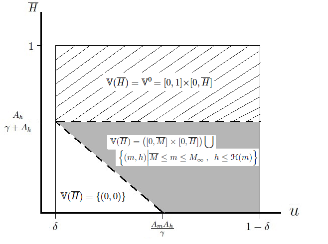
This new form (57) taken by the inequalities (55) allows us to visualize the relation between the maximum proportion H¯¯𝐻\overline{H} of infected humans and the maximum u¯¯𝑢\overline{u} mortality fumigation rate. Figure 6 displays the graph of H¯¯𝐻\overline{H} versus u¯¯𝑢\overline{u}.

Refer to caption
Figure 6: Viability kernel for the Ross-MacDonald model (1), in function of the cap H¯¯𝐻\overline{H} on the proportion of infected humans and of the maximum mortality rate u¯¯𝑢\overline{u} of mosquitoes

Equalities in the inequalities on both sides of (57) correspond to the two dashed straight lines on Figure 6.

L)

When the couple (u¯,H¯)¯𝑢¯𝐻(\overline{u},\overline{H}) belongs to the unshaded bottom triangle (corresponding to a low upper bound H¯¯𝐻\overline{H}), the viability kernel consists only of the origin.

H)

When the couple (u¯,H¯)¯𝑢¯𝐻(\overline{u},\overline{H}) belongs to the upper rectangle shaded with lines (corresponding to a high upper bound H¯¯𝐻\overline{H}), the viability kernel is the whole constraint set 𝕍0(H¯)=[0,1]×[0,H¯]superscript𝕍0¯𝐻010¯𝐻\mathbb{V}^{0}(\overline{H})=[0,1]\times[0,\overline{H}].

H)

When the couple (u¯,H¯)¯𝑢¯𝐻(\overline{u},\overline{H}) belongs to the the gray shaded region (corresponding to a medium upper bound H¯¯𝐻\overline{H}), the viability kernel is a strict subset of the constraint set 𝕍0(H¯)=[0,1]×[0,H¯]superscript𝕍0¯𝐻010¯𝐻\mathbb{V}^{0}(\overline{H})=[0,1]\times[0,\overline{H}], whose top right frontier is the smooth curve given in (56b).

3.5 Viable controls

After having characterized the viability kernel, we turn to discussing so-called viable controls. In viability theory [2], it is proven that any control u[u¯,u¯]𝑢¯𝑢¯𝑢u\in[\underline{u},\overline{u}], such that the vector (gm,gh)subscript𝑔𝑚subscript𝑔(g_{m},g_{h}) points towards the inside of the viability kernel 𝕍(H¯)𝕍¯𝐻\mathbb{V}(\overline{H}) is viable in the following sense: a trajectory of viable controls and an initial state in 𝕍(H¯)𝕍¯𝐻\mathbb{V}(\overline{H}) produce a state trajectory in 𝕍(H¯)𝕍¯𝐻\mathbb{V}(\overline{H}).

L)

With a strong constraint as in (51), it is impossible to keep the proportion of infected humans below H¯¯𝐻\overline{H} for all times, for whatever admissible control trajectory (5) (except if there are no infected humans or mosquitoes at the start), by Proposition 7.

H)

With a weak constraint as in (53), the constraint set 𝕍0(H¯)=[0,1]×[0,H¯]superscript𝕍0¯𝐻010¯𝐻\mathbb{V}^{0}(\overline{H})=[0,1]\times[0,\overline{H}] is strongly invariant, by Proposition 8. Therefore, any admissible control trajectory (5) makes it possible that the proportion of infected humans remains below H¯¯𝐻\overline{H} for all times. For instance, the minimum control u¯=δ¯𝑢𝛿\underline{u}=\delta, corresponding to natural death rate (hence to no control), is a viable control.

M)

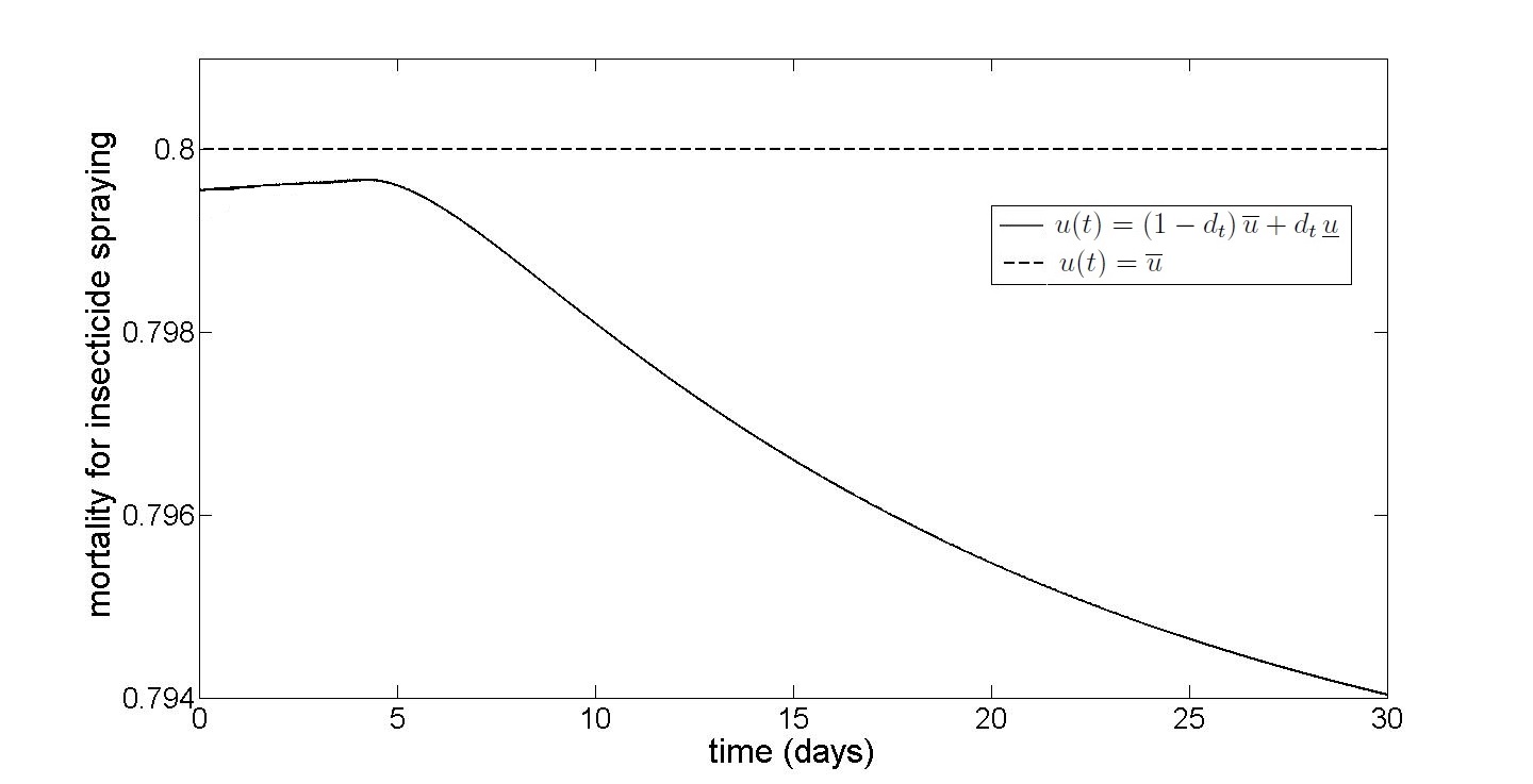
With a medium constraint as in (55), a viable control is the stationary control u()=u¯𝑢¯𝑢u(\cdot)=\overline{u}, corresponding to maximal fumigation. However, other controls might be viable: it suffices that, on the frontier of the viability kernel 𝕍(H¯)𝕍¯𝐻\mathbb{V}(\overline{H}), a control yields a vector (gm,gh)subscript𝑔𝑚subscript𝑔(g_{m},g_{h}) that points towards the inside of 𝕍(H¯)𝕍¯𝐻\mathbb{V}(\overline{H}). For instance, we could opt for a control which is low when far from the frontier of the viability kernel 𝕍(H¯)𝕍¯𝐻\mathbb{V}(\overline{H}), but reaches u¯¯𝑢\overline{u} when close to the frontier. Letting d(m,h)𝑑𝑚d(m,h) be the distance between point (m,h)𝑚(m,h) and the upper frontier of the viability kernel 𝕍(H¯)𝕍¯𝐻\mathbb{V}(\overline{H}), we propose the following viable control for problem (6):

u(t)=(1exp(d(m(t),h(t))))u¯+exp(d(m(t),h(t)))u¯.𝑢𝑡1𝑑𝑚𝑡𝑡¯𝑢𝑑𝑚𝑡𝑡¯𝑢u(t)=\Big{(}1-\exp\Big{(}-d\big{(}m(t),h(t)\big{)}\Big{)}\Big{)}\underline{u}+\exp\Big{(}-d\big{(}m(t),h(t)\big{)}\Big{)}\overline{u}\;. (58)

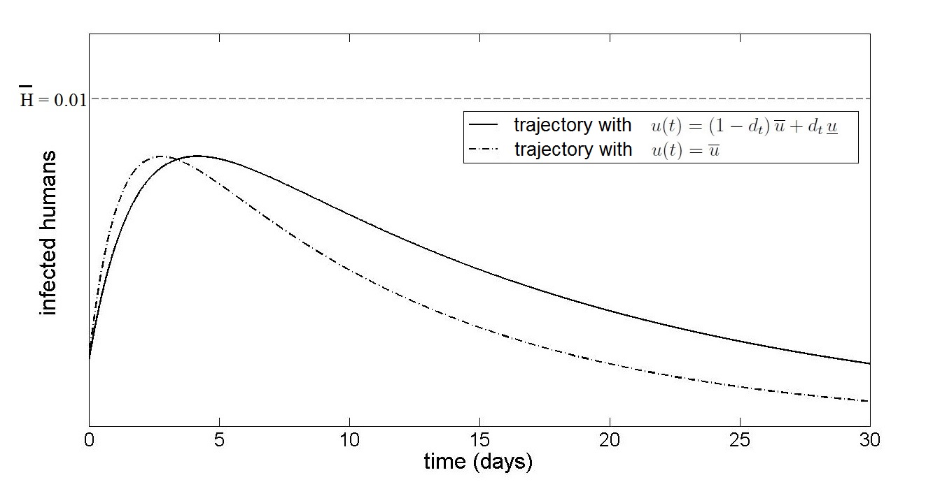
Figures 7 and 8 display examples of viable control and state (infected humans) trajectories for the Ross-MacDonald model (1) with a proportion of 1% infected humans not to be exceeded (H¯=0.01¯𝐻0.01\overline{H}=0.01).

Refer to caption
Figure 7: Viable control trajectories for the Ross-MacDonald model (1) with H¯=0.01¯𝐻0.01\overline{H}=0.01
Refer to caption
Figure 8: Viable state (infected humans) trajectories for the Ross-MacDonald model (1) with H¯=0.01¯𝐻0.01\overline{H}=0.01

4 Conclusion

As said in the introduction, the approach we have developed is (to our best knowledge) new in mathematical epidemiology. Instead of aiming at an equilibrium or optimizing, we have looked for policies able to maintain the infected individuals below a threshold for all times. More precisely, we have allowed for time-dependent fumigation rates to reduce the population of mosquito vector, in order to maintain the proportion of infected individuals by dengue below a threshold for all times. By definition, the viability kernel is the set of initial states (mosquitoes and infected individuals) for which such a fumigation control trajectory exists.

Our theoretical results are the following. For the Ross-Macdonald model with vector mortality control, we have been able to characterize the viability kernel associated with the viability constraint that consists in capping the proportion of infected humans for all times. Depending on whether the cap on the proportion of infected is low, high or medium, we have provided different expressions of the viability kernel. We have also characterized so-called viable policies that produce, at each time, a fumigation rate as a function of current proportions of infected humans and mosquitoes, such that the proportion of infected humans remains below a threshold for all times.

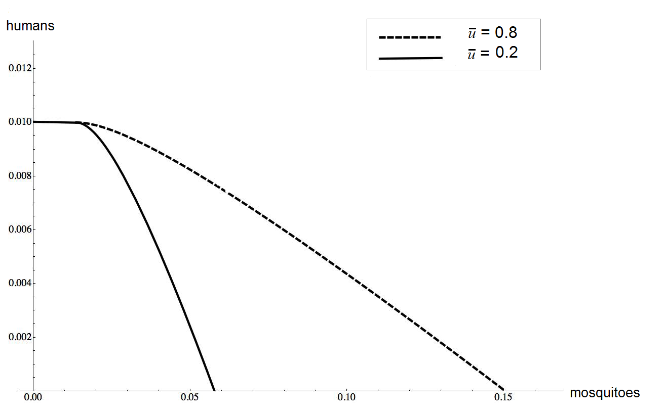
Regarding the use of our theoretical results, we have provided a numerical application in the case of the control of a dengue outbreak in 2013 in Cali, Colombia. Indeed, thanks to numerical data yielded by the Municipal Secretariat of Public Health of Cali, we have produced figures of viability kernels and of viable trajectories. What our analysis suggests is that, to cap the proportion of infected humans at the peak, you need to measure the proportion of infected mosquitoes, at least when it is larger than the characteristic proportion M¯¯𝑀\overline{M}, defined in (28). Measuring mosquito abundance is a difficult task, whereas measuring a proportion of infected mosquitoes might be done by proper sampling. Naturally, the weaker the control, the more you need to estimate the proportion of infected mosquitoes, as illustrated in Figure 9.
Refer to caption
Figure 9: Dependence of the viability kernel on the maximal fumigation mortality rate u¯¯𝑢\overline{u}

Appendix A Appendix

A.1 Recalls on comparison theorems for differential systems

Definition 15.

The function g:nn:𝑔superscript𝑛superscript𝑛g:\mathbb{R}^{n}\rightarrow\mathbb{R}^{n} is said to be quasi monotonous if g𝑔g is C1superscript𝐶1C^{1} and that

gixj0,ij.formulae-sequencesuperscript𝑔𝑖subscript𝑥𝑗0for-all𝑖𝑗\frac{\partial g^{i}}{\partial x_{j}}\geq 0\;,\enspace\forall i\neq j\;.

In what follows, all inequalities between vectors have to be understood componentwise.

Theorem 16.

Let f𝑓f and g𝑔g be two vector fields on Dn𝐷superscript𝑛D\subset\mathds{R}^{n}, with f𝑓f or g𝑔g quasi monotonous and fg𝑓𝑔f\leq g. Suppose that the differential systems

𝐱˙=f(𝐱),𝐲˙=g(𝐲),formulae-sequence˙𝐱𝑓𝐱˙𝐲𝑔𝐲\dot{\mathbf{x}}=f(\mathbf{x})\;,\enspace\dot{\mathbf{y}}=g(\mathbf{y})\;,

have solutions t𝐱tmaps-to𝑡subscript𝐱𝑡t\mapsto\mathbf{x}_{t} and t𝐲tmaps-to𝑡subscript𝐲𝑡t\mapsto\mathbf{y}_{t} defined for all t0𝑡0t\geq 0. Then, if 𝐱0𝐲0subscript𝐱0subscript𝐲0\mathbf{x}_{0}\leq\mathbf{y}_{0}, we have that 𝐱t𝐲tsubscript𝐱𝑡subscript𝐲𝑡\mathbf{x}_{t}\leq\mathbf{y}_{t} for all t0𝑡0t\geq 0.

Proof.

We consider two cases.

  1. (a)

    Suppose that f<g𝑓𝑔f<g — that is, fi<gisuperscript𝑓𝑖superscript𝑔𝑖f^{i}<g^{i} for all i=1,,n𝑖1𝑛i=1,\dots,n — and that 𝐱0<𝐲0subscript𝐱0subscript𝐲0\mathbf{x}_{0}<\mathbf{y}_{0}. We define

    τ=inf{t0i=1,,n,𝐱ti>𝐲ti}.𝜏infimumconditional-set𝑡0formulae-sequence𝑖1𝑛superscriptsubscript𝐱𝑡𝑖superscriptsubscript𝐲𝑡𝑖\tau=\inf\{t\geq 0\mid\exists i=1,\dots,n\;,\enspace\mathbf{x}_{t}^{i}>\mathbf{y}_{t}^{i}\}\;.

    We show that τ=+𝜏\tau=+\infty, that is, 𝐱t𝐲tsubscript𝐱𝑡subscript𝐲𝑡\mathbf{x}_{t}\leq\mathbf{y}_{t} for all t0𝑡0t\geq 0. Indeed, let us suppose the contrary. If τ<+𝜏\tau<+\infty, then there exists at least one i=1,,n𝑖1𝑛i=1,\dots,n such that

    𝐱τi=𝐲τi,𝐱τj𝐲τj,ji.formulae-sequencesubscriptsuperscript𝐱𝑖𝜏subscriptsuperscript𝐲𝑖𝜏formulae-sequencesubscriptsuperscript𝐱𝑗𝜏subscriptsuperscript𝐲𝑗𝜏for-all𝑗𝑖\mathbf{x}^{i}_{\tau}=\mathbf{y}^{i}_{\tau}\;,\enspace\mathbf{x}^{j}_{\tau}\leq\mathbf{y}^{j}_{\tau}\;,\enspace\forall j\neq i\;.

    Supposing that g𝑔g is quasi monotonous (the proof is similar when f𝑓f is quasi monotonous), we deduce that gi(𝐱τ)gi(𝐲τ)superscript𝑔𝑖subscript𝐱𝜏superscript𝑔𝑖subscript𝐲𝜏g^{i}(\mathbf{x}_{\tau})\leq g^{i}(\mathbf{y}_{\tau}).

    Moreover, as 𝐱ti>𝐲tisuperscriptsubscript𝐱𝑡𝑖superscriptsubscript𝐲𝑡𝑖\mathbf{x}_{t}^{i}>\mathbf{y}_{t}^{i}, for all t]τ,τ+ϵ[t\in]\tau,\tau+\epsilon[ (for ϵitalic-ϵ\epsilon small enough) and 𝐱τi=𝐲τisubscriptsuperscript𝐱𝑖𝜏subscriptsuperscript𝐲𝑖𝜏\mathbf{x}^{i}_{\tau}=\mathbf{y}^{i}_{\tau}, we have that

    fi(𝐱τ)=d𝐱tidt|t=τd𝐲tidt|t=τ=gi(𝐲τ).f^{i}(\mathbf{x}_{\tau})=\frac{d\mathbf{x}_{t}^{i}}{dt}_{|t=\tau}\geq\frac{d\mathbf{y}_{t}^{i}}{dt}_{|t=\tau}=g^{i}(\mathbf{y}_{\tau})\;.

    From gi(𝐱τ)gi(𝐲τ)superscript𝑔𝑖subscript𝐱𝜏superscript𝑔𝑖subscript𝐲𝜏g^{i}(\mathbf{x}_{\tau})\leq g^{i}(\mathbf{y}_{\tau}), gi(𝐲τ)fi(𝐱τ)superscript𝑔𝑖subscript𝐲𝜏superscript𝑓𝑖subscript𝐱𝜏g^{i}(\mathbf{y}_{\tau})\leq f^{i}(\mathbf{x}_{\tau}) and fi<gisuperscript𝑓𝑖superscript𝑔𝑖f^{i}<g^{i}, we deduce that

    gi(𝐱τ)gi(𝐲τ)fi(𝐱τ)<gi(𝐱τ).superscript𝑔𝑖subscript𝐱𝜏superscript𝑔𝑖subscript𝐲𝜏superscript𝑓𝑖subscript𝐱𝜏superscript𝑔𝑖subscript𝐱𝜏g^{i}(\mathbf{x}_{\tau})\leq g^{i}(\mathbf{y}_{\tau})\leq f^{i}(\mathbf{x}_{\tau})<g^{i}(\mathbf{x}_{\tau})\;.

    This is contradictory. As a consequence, 𝐱0<𝐲0subscript𝐱0subscript𝐲0\mathbf{x}_{0}<\mathbf{y}_{0} implies that 𝐱t𝐲tsubscript𝐱𝑡subscript𝐲𝑡\mathbf{x}_{t}\leq\mathbf{y}_{t} for all t0𝑡0t\geq 0.

  2. (b)

    Suppose that fg𝑓𝑔f\leq g and 𝐱0𝐲0subscript𝐱0subscript𝐲0\mathbf{x}_{0}\leq\mathbf{y}_{0}. For any ϵ>0italic-ϵ0\epsilon>0, denote by 𝐲tϵsuperscriptsubscript𝐲𝑡italic-ϵ\mathbf{y}_{t}^{\epsilon} the solution of

    𝐲ϵ˙=g(𝐲ϵ)+ϵ,𝐲0ϵ=𝐲0+ϵ.formulae-sequence˙superscript𝐲italic-ϵ𝑔superscript𝐲italic-ϵitalic-ϵsubscriptsuperscript𝐲italic-ϵ0subscript𝐲0italic-ϵ\dot{\mathbf{y}^{\epsilon}}=g(\mathbf{y}^{\epsilon})+\epsilon\;,\enspace\mathbf{y}^{\epsilon}_{0}=\mathbf{y}_{0}+\epsilon\;.

    We have that

    𝐱0<𝐲0ϵ,f<g+ϵ.formulae-sequencesubscript𝐱0subscriptsuperscript𝐲italic-ϵ0𝑓𝑔italic-ϵ\mathbf{x}_{0}<\mathbf{y}^{\epsilon}_{0}\;,\enspace f<g+\epsilon\;.

    Therefore, we can conclude from the previous item that 𝐱t𝐲tϵsubscript𝐱𝑡subscriptsuperscript𝐲italic-ϵ𝑡\mathbf{x}_{t}\leq\mathbf{y}^{\epsilon}_{t} for all t0𝑡0t\geq 0. It is well known that, for fixed t𝑡t, when ϵ0italic-ϵ0\epsilon\downarrow 0, we have that 𝐲tϵ𝐲tsubscriptsuperscript𝐲italic-ϵ𝑡subscript𝐲𝑡\mathbf{y}^{\epsilon}_{t}\rightarrow\mathbf{y}_{t}.

    As a consequence, 𝐱0𝐲0subscript𝐱0subscript𝐲0\mathbf{x}_{0}\leq\mathbf{y}_{0} implies that 𝐱t𝐲tsubscript𝐱𝑡subscript𝐲𝑡\mathbf{x}_{t}\leq\mathbf{y}_{t} for all t0𝑡0t\geq 0.

The following extension is immediate.

Theorem 17.

Let (ft)t0subscriptsubscript𝑓𝑡𝑡0(f_{t})_{t\geq 0} and (gt)t0subscriptsubscript𝑔𝑡𝑡0(g_{t})_{t\geq 0} be two families of vector fields on Dn𝐷superscript𝑛D\subset\mathds{R}^{n}, with ftsubscript𝑓𝑡f_{t} or gtsubscript𝑔𝑡g_{t} quasi monotonous and ftgtsubscript𝑓𝑡subscript𝑔𝑡f_{t}\leq g_{t}, for all t0𝑡0t\geq 0. Suppose that the differential systems

𝐱˙=ft(𝐱),𝐲˙=gt(𝐲),formulae-sequence˙𝐱subscript𝑓𝑡𝐱˙𝐲subscript𝑔𝑡𝐲\dot{\mathbf{x}}=f_{t}(\mathbf{x})\;,\enspace\dot{\mathbf{y}}=g_{t}(\mathbf{y})\;,

have solutions t𝐱tmaps-to𝑡subscript𝐱𝑡t\mapsto\mathbf{x}_{t} and t𝐲tmaps-to𝑡subscript𝐲𝑡t\mapsto\mathbf{y}_{t} defined for all t0𝑡0t\geq 0. Then, if 𝐱0𝐲0subscript𝐱0subscript𝐲0\mathbf{x}_{0}\leq\mathbf{y}_{0}, we have that 𝐱t𝐲tsubscript𝐱𝑡subscript𝐲𝑡\mathbf{x}_{t}\leq\mathbf{y}_{t} for all t0𝑡0t\geq 0.

A.2 Epidemic model adjusted to 2013 dengue outbreak in Cali, Colombia

The city of Cali, in Colombia, has witnessed several episodes of dengue, as displayed in Figure 10.
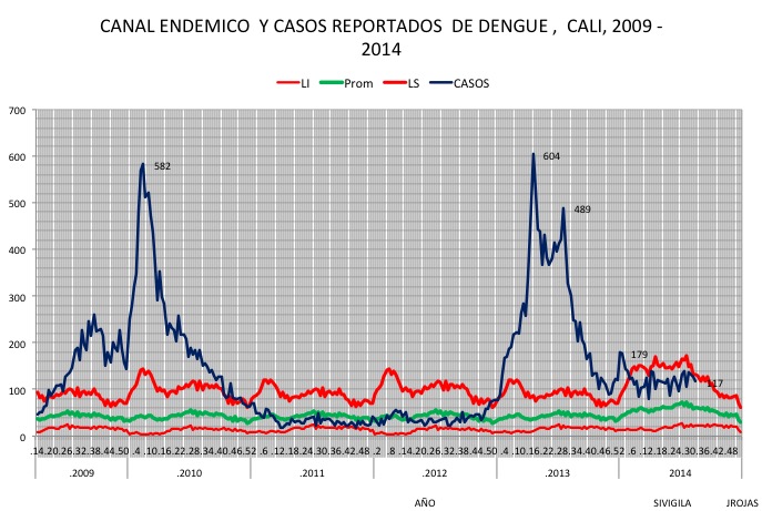
Refer to caption
Figure 10: Number of infected by dengue, revealing several episodes of dengue in the city of Cali, in Colombia

The Municipal Secretariat of Public Health of Cali provided us with data corresponding to the dengue outbreak registered in 2013. Here, we present how we have estimated the parameters in the Ross-Macdonal model (1) — using the information of daily reports for new registered cases of dengue in Cali — to obtain different figures of viability kernels and of viable trajectories.

Definition of parameters

We introduce the state vector

z(t)=(m(t),h(t))[0,1]2,𝑧𝑡𝑚𝑡𝑡superscript012z(t)=\big{(}m(t),h(t)\big{)}\in[0,1]^{2}\;, (59)

and the vector of parameters

θ=(α,ph,pm,ξ,δ)Θ+5,𝜃𝛼subscript𝑝subscript𝑝𝑚𝜉𝛿Θsubscriptsuperscript5\theta=\big{(}\alpha,p_{h},p_{m},\xi,\delta\big{)}\in\Theta\subset\mathbb{R}^{5}_{+}\;, (60)

consisting of the five parameters previously defined in Table 1. The parameter set Θ+5Θsubscriptsuperscript5\Theta\subset\mathbb{R}^{5}_{+} is given by the Cartesian product of the five intervals in the third column of Table 2.

With these notations, the Ross-Macdonal model (1) now writes

ddtz(t;θ)=𝐟(z(t;θ),θ)t>0z(0;θ)=z0z0=(m0,h0)𝑑𝑑𝑡𝑧𝑡𝜃𝐟𝑧𝑡𝜃𝜃missing-subexpression𝑡0𝑧0𝜃subscript𝑧0missing-subexpressionsubscript𝑧0superscriptsubscript𝑚0subscript0\begin{array}[]{rclcl}\dfrac{d}{dt}z(t;\theta)&=&\mathbf{f}\big{(}z(t;\theta),\theta\big{)}&&t>0\\ z(0;\theta)&=&z_{0}&&z_{0}=(m_{0},h_{0})^{\prime}\end{array} (61)

where

𝐟(z,θ)=(f1(z,θ)f2(z,θ))=(αpmh(1m)δmαphξm(1h)γh),γ=0.1.formulae-sequence𝐟𝑧𝜃subscript𝑓1𝑧𝜃subscript𝑓2𝑧𝜃𝛼subscript𝑝𝑚1𝑚𝛿𝑚𝛼subscript𝑝𝜉𝑚1𝛾𝛾0.1\mathbf{f}(z,\theta)=\left(\begin{array}[]{c}f_{1}(z,\theta)\\ f_{2}(z,\theta)\end{array}\right)=\left(\begin{array}[]{c}\alpha\,p_{m}\,h(1-m)-\delta\,m\\ \alpha\,p_{h}\,\xi\,m(1-h)-\gamma\,h\end{array}\right)\;,\gamma=0.1\;. (62)

Daily data deduced from health reports

Notice that the rate γ𝛾\gamma of human recovery does not appear in the parameter vector θ𝜃\theta in (60). Indeed, in the data we only have new cases of dengue registered per day; there is no information regarding how many people recover daily. We chose an infectiousness period of 10 days, that is, a rate of human recovery fixed at γ=0.1𝛾0.1\gamma=0.1. Under this assumption, the daily incidence data (i.e., numbers of newly registered cases reported on daily basis) provided by the Municipal Secretariat of Public Health (Cali, Colombia) can be converted into the daily prevalence data (i.e., numbers of infected people on a given day, be they new or not). With this, we deduce values of daily proportion of infected people in the form of the set

𝕆={(tj,h^j),j=0,1,,𝒟},\mathbb{O}=\Big{\{}\big{(}t_{j},\widehat{h}_{j}\big{)}\;,\enspace j=0,1,\ldots,\mathcal{D}\Big{\}}\;, (63)

where tjsubscript𝑡𝑗t_{j} refers to j𝑗j-th day, within the observation period of (𝒟+1)𝒟1(\mathcal{D}+1) days, and where h^jsubscript^𝑗\widehat{h}_{j} stands for the fraction of infected people at the day tjsubscript𝑡𝑗t_{j}. Naturally, the first couple in the set (63) defines the initial condition h(t0)=h^0subscript𝑡0subscript^0h(t_{0})=\widehat{h}_{0} with t0=0subscript𝑡00t_{0}=0 (initial observation day). Unfortunately, there is no available data for the fraction of infected mosquitoes. As mosquito abundance is strongly correlated with dengue outbreaks [21], we have chosen a linear relation m(0)=3h^0𝑚03subscript^0m(0)=3\widehat{h}_{0} at the beginning of an epidemic outburst (other choices gave similar numerical results).

Parameter estimation procedure

To estimate a parameter vector θΘ𝜃Θ\theta\in\Theta that suits with the data, we have applied the curve-fitting approach based on least-square method. More precisely, we look for an optimal solution to the problem of constrained optimization

minθΘφ(θ)=12j=1𝒟(h(tj,θ)h^j)2,𝒟=60days,formulae-sequencesubscript𝜃Θ𝜑𝜃12superscriptsubscript𝑗1𝒟superscriptsubscript𝑡𝑗𝜃subscript^𝑗2𝒟60days\min\limits_{\theta\in\Theta}\varphi(\theta)=\frac{1}{2}\sum\limits_{j=1}^{\mathcal{D}}\,\big{(}h(t_{j},\theta)-\widehat{h}_{j}\big{)}^{2},\quad\mathcal{D}=60\;\mbox{days}\;, (64)

subject to the differential constraint (61). Regarding numerics, we have solved this optimization problem with the lsqcurvefit routine (MATLAB Optimization Toolbox), starting with an admissible θ0Θsubscript𝜃0Θ\theta_{0}\in\Theta (see its exact value in Table 2, second column). The routine generates a sequence {θ1,θ2,}subscript𝜃1subscript𝜃2\{\theta_{1},\theta_{2},\ldots\} that we stop once it is stationary, up to numerical precision. For a better result, we have combined two particular methods (Trust-Region-Reflective Least Squares Algorithm [29] and Levenberg-Marquardt Algorithm [25]) in the implementation of the lsqcurvefit MATLAB routine.

Parameter Initial value Range Reference Estimated value
α𝛼\alpha 1 [0,5]05[0,5] [11, 26] 0,3365
pmsubscript𝑝𝑚p_{m} 0.5 [0,1]01[0,1] 0,1532
phsubscript𝑝p_{h} 0.5 [0,1]01[0,1] 0,2287
ξ𝜉\xi 1 [1,5]15[1,5] [24, 27] 1,0359
δ𝛿\delta 0.035 [130,115]130115\left[\frac{1}{30},\frac{1}{15}\right] [11, 27] 0.0333
Table 2: Initial values, admissible ranges, respective source references, and estimated values of parameters (numerical solution of optimization problem (64)).

The last column of Table 2 provides estimated values for the parameters θ=(α,ph,pm,ξ,δ)𝜃𝛼subscript𝑝subscript𝑝𝑚𝜉𝛿\theta=\big{(}\alpha,p_{h},p_{m},\xi,\delta\big{)}, and Figure 11 displays the curve-fitting results.
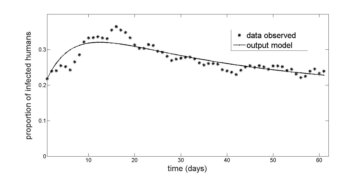
Refer to caption
Figure 11: Fraction of people infected with dengue obtained by adjustment of the Ross-Macdonal model (1) (smooth solid curve) versus registered daily prevalence cases (star isolated points) during the 2013 dengue outbreak in Cali, Colombia
Acknowledgments.

The authors thank the French program PEERS-AIRD (Modèles d’optimisation et de viabilité en écologie et en économie) and the Colombian Programa Nacional de Ciencias Básicas COLCIENCIAS (Modelos y métodos matemáticos para el co trol y vigilancia del dengue, código 125956933846) that offered financial support for missions, together with École des Ponts ParisTech (France), Université Paris-Est (France), Universidad Autónoma de Occidente (Cali, Colombia) and Universidad del Valle (Cali, Colombia).

References

  • [1] R. M. Anderson and R. M. May. Infectious Diseases of Humans: Dynamics and Control. Oxford Science Publications. OUP Oxford, 1992.
  • [2] J. P. Aubin. Viability theory. Systems & Control: Foundations & Applications. Birkhäuser Boston Inc., Boston, MA, 1991.
  • [3] C. Béné, L. Doyen, and D. Gabay. A viability analysis for a bio-economic model. Ecological Economics, 36:385–396, 2001.
  • [4] D. Bertsekas and I. Rhodes. On the minimax reachability of target sets and target tubes. Automatica, 7:233–247, 1971.
  • [5] G. Bitsoris. On the positive invariance of polyhedral sets for discrete-time systems. Systems and Control Letters, 11(3):243–248, 1988.
  • [6] F. Blanchini. Set invariance in control (survey paper). Automatica, 35(11):1747–1767, 1999.
  • [7] N. Bonneuil and K. Müllers. Viable populations in a prey-predator system. Journal of Mathematical Biology, 35(3):261–293, February 1997.
  • [8] N. Bonneuil and P. Saint-Pierre. Population viability in three trophic-level food chains. Applied Mathematics and Computation, 169(2):1086 – 1105, 2005.
  • [9] F. Brauer and C. Castillo-Chávez. Mathematical models in population biology and epidemiology, volume 40 of Texts in Applied Mathematics. Springer-Verlag, New York, 2001.
  • [10] F. H. Clarke, Y. S. Ledayev, R. J. Stern, and P. R. Wolenski. Qualitative properties of trajectories of control systems: a survey. Journal of Dynamical Control Systems, 1:1–48, 1995.
  • [11] A. Costero, J. D. Edman, G. G. Clark, and T. W. Scott. Life table study of Aedes aegypti (diptera: Culicidae) in Puerto Rico fed only human blood plus sugar. Journal of Medical Entomology, 35(5), 1998.
  • [12] R. V. Culshaw, S. Ruan, and R. J. Spiteri. Optimal HIV treatment by maximising immune response. Journal of Mathematical Biology, 48(5):545–562, 2004.
  • [13] M. De Lara and L. Doyen. Sustainable Management of Natural Resources. Mathematical Models and Methods. Springer-Verlag, Berlin, 2008.
  • [14] O. Diekmann and J. A. P. Heesterbeek. Mathematical Epidemiology of Infectious Diseases. Wiley, Utrecht, Netherland, 2000.
  • [15] E. G. Gilbert and K. T. Tan. Linear systems with state and control constraints: the theory and application of maximal output admissible sets. IEEE Transactions on Automatic Control, 36(9):1008–1020, 1991.
  • [16] P.-O. Gutman and M. Cwikel. Admissible sets and feedback control for discrete-time linear dynamical systems with bounded controls and states. IEEE Transactions on Automatic Control, 31(4):373– 376, 1986.
  • [17] E. Hansen and T. Day. Optimal control of epidemics with limited resources. Journal of Mathematical Biology, pages 1–29, 2010.
  • [18] H. W. Hethcote. Optimal ages of vaccination for measles. Mathematical Biosciences, 89(1):29 – 52, 1988.
  • [19] H. W. Hethcote. The mathematics of infectious diseases. SIAM Review, 42:599–653, 2000.
  • [20] H. W. Hethcote and P. Waltman. Optimal vaccination schedules in a deterministic epidemic model. Mathematical Biosciences, 18(3-4):365 – 381, 1973.
  • [21] C. C. Jansen and N. W. Beebe. The dengue vector Aedes aegypti: what comes next. Microbes and infection, 12(4):272–279, 2010.
  • [22] D. Kirschner, S. Lenhart, and S. Serbin. Optimal control of the chemotherapy of HIV. Journal of Mathematical Biology, 35(7):775–792, 1997.
  • [23] I. M. Longini Jr, E. Ackerman, and L. R. Elveback. An optimization model for influenza A epidemics. Mathematical Biosciences, 38(1-2):141 – 157, 1978.
  • [24] F. Méndez, M. Barreto, J. F. Arias, G. Rengifo, J. Muñoz, M. E. Burbano, and B. Parra. Human and mosquito infections by dengue viruses during and after epidemics in a dengue-endemic region of Colombia. Am J Trop Med Hyg., 74(4):678–683, 2006.
  • [25] J. J. Moré. The Levenberg-Marquardt algorithm: implementation and theory. In Numerical analysis, pages 105–116. Springer, 1978.
  • [26] T. W. Scott, P. Amerasinghe, A. C. Morrison, L. H. Lorenz, G. G. Clark, D. Strickman, P. Kittayapong, and J. D. Edman. Longitudinal studies of Aedes aegypti (Diptera: Culicidae) in Thailand and Puerto Rico: blood feeding frequency. Journal of medical entomology, 37(1):89–101, 2000.
  • [27] T. W. Scott, A. C. Morrison, L. H. Lorenz, G. G. Clark, D. Strickman, P. Kittayapong, H. Zhou, and J. D. Edman. Longitudinal studies of Aedes aegypti (Diptera: Culicidae) in Thailand and Puerto Rico: population dynamics. Journal of medical entomology, 37(1):77–88, 2000.
  • [28] D. L. Smith, F. E. McKenzie, R. W. Snow, and S. I. Hay. Revisiting the basic reproductive number for malaria and its implications for malaria control. PLoS Biol, 5(3):e42, 02 2007.
  • [29] D. C. Sorensen. Newton’s method with a model trust region modification. SIAM Journal on Numerical Analysis, 19(2):409–426, 1982.
  • [30] W. Walter. Ordinary Differential Equations. Graduate Texts in Mathematics. Springer New York, 1998.