Entangled collective-spin states of atomic ensembles under non-uniform atom-light interaction
Abstract
We consider the optical generation and verification of entanglement in atomic ensembles under non-uniform interaction between the ensemble and an optical mode. We show that for a wide range of parameters a system of non-uniformly coupled atomic spins can be described as an ensemble of uniformly coupled spins with a reduced effective atom-light coupling and a reduced effective atom number, with a reduction factor of order unity given by the ensemble-mode geometry. This description is valid even for complex entangled states with arbitrary phase-space distribution functions as long as the detection does not resolve single spins. Furthermore, we derive an analytic formula for the observable entanglement in the case, of relevance in practice, where the ensemble-mode coupling differs between state generation and measurement.
pacs:
42.50.Dv,42.50.Pq,37.30.+iI Introduction
In cavity quantum electrodynamics (cQED), an optical resonator enhances the interaction between atoms and light. A particularly interesting regime is reached when the back action of the atoms on the cavity and the back action of the cavity field on the atoms become appreciable. In this strong-coupling regime where the system can evolve reversibly and coherently, many interesting experiments can be realized Turchette et al. (1995); Birnbaum et al. (2005); Colombe et al. (2007); Chen et al. (2011); Haas et al. (2014); Schleier-Smith et al. (2010); Leroux et al. (2010a). For instance, it is possible to realize measurements beyond the standard quantum limit Chen et al. (2011); Schleier-Smith et al. (2010); Leroux et al. (2010a); Bohnet et al. (2014) by preparing a particular class of entangled states, spin squeezed states. These states are typically prepared using a non-uniform light-atom interaction. Recently, a different entangled state of many atoms described by a negative-valued, doughnut-shaped Wigner function has been realized using the strong collective light-atom interaction in a standing-wave optical cavity with manifestly non-uniform atom-light coupling McConnell et al. (2015).
Most treatments of atom-light coupling Kitagawa and Ueda (1993); Bollinger et al. (1996); Chen et al. (2014); McConnell et al. (2013) consider the situation where the atoms and light are uniformly coupled. However, in real systems, this assumption is hardly ever fulfilled. For instance, when the atomic cloud is comparable to or larger than the waist of the light mode to which the atoms are coupled, it is necessary to take into account the inhomogeneity of the atom-light coupling caused by the mode profile. In general, when the light intensity is not uniform in the volume occupied by the atoms, non-uniform atom-light coupling occurs. While this could be remedied by using a larger beam, this is often undesirable, as it reduces the strength of the atom-light interaction Tanji-Suzuki et al. (2011). More generally, the coupling is always non-uniform at some level, for instance, due to thermal motion of the atoms. The effect of inhomogeneous coupling is more severe for highly entangled states.
Theoretical work on non-uniformly coupled atom-light systems has focused on Gaussian states Kuzmich and Kennedy (2004); Madsen and Mølmer (2004); López et al. (2007) , where the atomic quasi probability function is described by a Gaussian function. However, it is not immediately obvious whether non-Gaussian entangled states McConnell et al. (2013); Haas et al. (2014); McConnell et al. (2015); Strobel et al. (2014); Christensen et al. (2013, 2014) can be generated and detected under non-uniform atom-light coupling.
For uniform coupling, the collective spin degrees of freedom are well described by the total spin components , and , with the eigenstates of (or , ) being the Dicke states Dicke (1954). The question then is whether similar collective operators can be found to describe the evolution and measurement of the collective spin under non-uniform coupling.
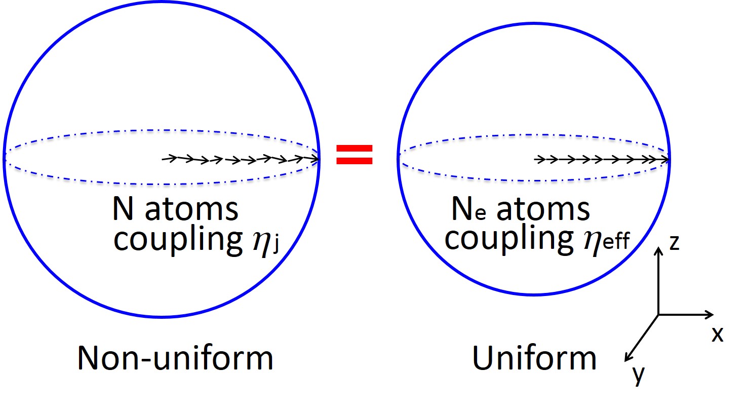
In this article, we prove that for a wide range of states the non-uniformly coupled system is equivalent to a (slightly smaller) uniformly coupled system when the atom number is large, and when the individual atomic spins are mostly aligned with each other, i.e. , where is the spin of a single atom. We show that under a wide range of conditions, we can simply replace the spin operator , , by appropriately defined effective spin operators , , to describe the system. The system dynamics are then the same as those of a uniformly coupled system. We also define effective Dicke states under non-uniform coupling, and generalize the concept of the effective atom number that was first introduced in Ref Schleier-Smith et al. (2010); Leroux et al. (2010a), and that has been applied to several experiments Bohnet et al. (2014); Leroux et al. (2010b); McConnell et al. (2013).
II The equivalence between uniform and non-uniform coupling
To be specific, we consider here the quantum non-demolition interaction that is used for most experiments Haas et al. (2014); Chen et al. (2011); Schleier-Smith et al. (2010); Bohnet et al. (2014); Leroux et al. (2010a); McConnell et al. (2015); Chen et al. (2014) such as spin squeezing and entangled states generation. It has the form
| (1) |
Here, , where is the spin operator along the axis of atom , and is any Hermitian operator of the light field.
A Hamiltonian of this form appears in a variety of situations. For instance, if Schleier-Smith et al. (2010); Leroux et al. (2010a); Chen et al. (2011); Bohnet et al. (2014), which is the intensity operator of the light, where is the annihilation operator for a photon in the electromagnetic mode of interest, then describes the shift of the cavity resonance frequency by the atoms, or equivalently, the light shift on the atoms by the intracavity field. If Christensen et al. (2013, 2014); McConnell et al. (2015); Kuzmich and Kennedy (2004); Madsen and Mølmer (2004), which is the Stokes vector of light, then describes the polarization rotation by the atoms (Faraday rotation).
In the non-uniformly coupled system of atoms, the Hamiltonian of Eq. 1 becomes
| (2) |
where is the coupling strength of atom that is proportional to the local light intensity. If we are probing the atoms with a standing-wave beam in an optical resonator on the resonator axis, where is the position of the -th atom. If the probing beam is a Gaussian beam in free space or in a running-wave cavity, , where is the beam waist.
II.1 Special case of uniform atom-light coupling
We first discuss the case of uniform coupling and then generalize the results to non-uniform coupling. Let us define collective spin operators by
| (3) |
Here . Similarly, we generalize the definition of the raising and lowering spin operators along the axis by
| (4) | |||
| (5) |
Here, is the spin raising (lowering) operator for atom and . Any atomic state can be decomposed into a combination of different eigenstates of and , namely the Dicke states Dicke (1954).
Using the Holstein-Primakoff transformation Holstein and Primakoff (1940), when , we treat as the ground state and write creation and annihilation operators as
| (6) | |||
| (7) |
These operators satisfy the boson commutation relation . For convenience of notation, we replace () by () in the following.
It is straightforward to verify that the -th excited state
is the -th Dicke state of the atomic ensemble. It is also easy to show that the ground states of the Dicke manifold with total spin Dicke (1954), where , and are integers, can be generalized as . The corresponding excited Dicke states are given by . Using this formula, due to , we expect the -th excited state of the symmetric manifold to have approximately the same spin distribution probability as along any axis in the plane as long as .
As long as the curvature of the Bloch sphere can be neglected, i.e. and , the spin states can be mapped locally onto harmonic oscillator states Arecchi et al. (1972). Then for the state the probability amplitude to observe a spin in the measurement along the axis is
| (8) |
where is the -th order Hermite polynomial.
II.2 The generalization to non-uniform coupling
Now we generalize the above expressions for the case of non-uniform coupling. For a given Hamiltonian , we define the effective spin operators , for , , .
In order to preserve the commutation relation and the Heisenberg uncertainty principle, we require . Therefore we define the effective coupling as Schleier-Smith et al. (2010)
| (9) |
The collective creation and annihilation operators are defined in a similar way:
| (10) | |||
| (11) |
satisfies , and for and , we choose . For the other , we are not interested in the explicit expressions, as linear algebra theory guarantees the existence of these coefficients. commutes with any or () for , so any initial states will remain on the same Bloch sphere under the action of the Hamiltonian.
In this situation, we can define effective Dicke states which have the same observable properties as the Dicke states under uniform coupling.
| (12) |
where is the effective total spin which will be defined later.
Using the interaction described by the Hamiltonian in Eq 2, measurement of the observable yields information about . By applying an externally driven rotation along , one can measure , and we label this measurement as . As long as the resolution is not high enough to distinguish each individual spin, which is common in an atomic ensemble, the collective spin can be treated as a continuous variable Madsen and Mølmer (2004). So the probability amplitude to measure a particular is
| (13) |
Here, , is the effective atom number, and is the effective total spin. The idea of an effective atom number was first introduced in Refs Leroux et al. (2010a); Schleier-Smith et al. (2010) for characterizing Gaussian spin distribution, and we have derived it here more generally from the Heisenberg uncertainty.
Therefore, by using effective operators and an effective atom number, the physical observables remain the same as under uniform coupling. The equivalence also applies to any atomic states satisfying . The Hamiltonian is simply written as where . Then, all the predictions for the non-uniform coupling are equivalent to those for uniform coupling.
II.3 Connecting different coupling modes
Based on the analysis above, we can also derive a useful formula connecting different effective Dicke states. If we have two Hamiltonians with different atom-light coupling and , then we can define two sets of creation and annihilation operators and as above. For , we still have
| (14) | |||
| (15) |
We define the overlap parameter between these two couplings as
| (16) |
Without losing generality, we can choose the coefficients of the set such that .
Now we consider the state that is prepared on the maximal Bloch sphere of . Any effective Dicke state on this sphere can be expanded as
Applying this formula, we need to know just one parameter to establish the connection between effective Dicke states for different non-uniform coupling bases.
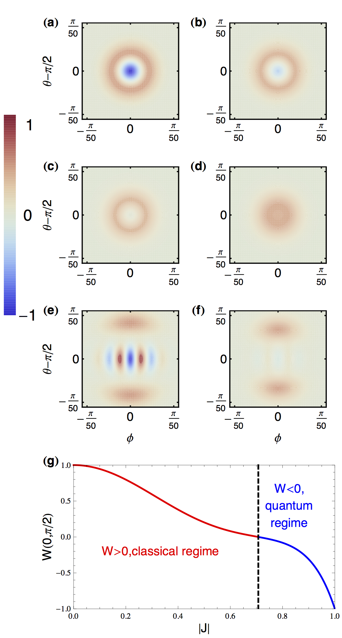
In Fig 2, we show a few examples illustrating the effects of non-uniform coupling. If we prepare and probe the first Dicke state with the same non uniform coupling, the Wigner function distribution reaches -1, the most non-classical value, and is identical to the Wigner function for uniform coupling. However, if we were to measure the same state in another coupling basis, we would find a reduced value for the magnitude of the negative Wigner function at the origin. If the overlap parameter is decreased further, the central hole in the Wigner function will be smeared out by the growing mismatch between the couplings used for state preparation and observation, respectively. Moreover, this effect is more obvious for a cat state in Fig, 2(e), (f), since the narrower fringes are more fragile than a wide hole. In fact, there is a general relation for any quantum state. When is below , the Wigner function is all positive, which corresponds to a classical probability distribution. Quantum interference with can only be seen when .
Another interesting example is the squeezed state. If the preparation and readout couplings are identical, the non-uniform coupling will not affect the squeezing parameter. The theoretical prediction and analysis under uniform coupling are still valid. The only correction needed is to replace the atom number by the effective atom number Schleier-Smith et al. (2010); Leroux et al. (2010a).
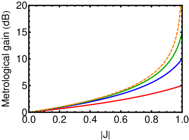
If there are different couplings involved in generating and observing in the squeezed state, the squeezing parameter will decrease when . In this case, the observable squeezing and the metrological gain are limited by the coupling overlap . For any given , there is always an upper bound of the metrological gain for any squeezed state. The results are summarized in Fig 3. This limitation could be important, e.g., for the operation of spin squeezed atom interferometers, where the atoms may be detected in a different position than where they were prepared.
Consider a squeezed state that approaches the Heisenberg limit, . The scaling of variance becomes instead of . However, the mismatch, due to effects such as atomic thermal motion, limits the detectable squeezing when we use this state in a precision measurement. We find that when , the best observable squeezing during the readout deteriorates to . The variance now scales again as , not . This shows that any change in the atom-light coupling between state preparation and readout larger than will destroy the Heisenberg-limited scaling. We use atoms trapped in an optical cavity as an example to illustrate the effect of finite temperature. We assume that the dipole trap used to confine the atoms and the probing light field have the same spatial mode. The thermal random motion reduces the parameter as , where is the temperature and is the trap depth. In order to observe the Heisenberg limit, the required temperature is below . For a trap depth of 10MHz and atoms, the ensemble must be cooled down to 100 nK to reach the Heisenberg limit.
III Conclusion
In conclusion, we have shown the equivalence between uniform coupling and non-uniform coupling in the optical preparation and detection of collective atomic spin states as long as no measurements with single-atom resolution are performed. This eliminates some conceptional concerns about entanglement in real, non-uniformly coupled systems. By using the effective spin and atom number, the collective evolution of the system can be described and predicted. We also derive a useful formula that can be used to calculate, e.g. the observable squeezing at finite atomic temperature or when an entangled atomic state is prepared with a different light mode than used for detection, e.g. in an atom interferometer Dimopoulos et al. (2007).
IV Acknowledgement
This work was supported by the NSF, DARPA (QUASAR), and MURI grants through AFOSR and ARO.
References
- Turchette et al. (1995) Q. A. Turchette, C. J. Hood, W. Lange, H. Mabuchi, and H. J. Kimble, Phys. Rev. Lett. 75, 4710 (1995).
- Birnbaum et al. (2005) K. M. Birnbaum, A. Boca, R. Miller, A. D. Boozer, T. E. Northup, and H. J. Kimble, Nature 436, 87 (2005).
- Colombe et al. (2007) Y. Colombe, T. Steinmetz, G. Dubois, F. Linke, D. Hunger, and J. Reichel, Nature 450, 272 (2007).
- Chen et al. (2011) Z. Chen, J. G. Bohnet, S. R. Sankar, J. Dai, and J. K. Thompson, Phys. Rev. Lett. 106, 133601 (2011).
- Haas et al. (2014) F. Haas, J. Volz, R. Gehr, J. Reichel, and J. Esteve, Science 344, 180 (2014).
- Schleier-Smith et al. (2010) M. H. Schleier-Smith, I. D. Leroux, and V. Vuletić, Phys. Rev. Lett. 104, 073604 (2010).
- Leroux et al. (2010a) I. D. Leroux, M. H. Schleier-Smith, and V. Vuletić, Phys. Rev. Lett. 104, 073602 (2010a).
- Bohnet et al. (2014) J. G. Bohnet, K. C. Cox, M. A. Norcia, J. M. Weiner, Z. Chen, and J. K. Thompson, Nature Photonics 8, 731 (2014).
- McConnell et al. (2015) R. McConnell, H. Zhang, J. Hu, S. Cuk, and V. Vuletic, Nature 519, 439 (2015).
- Kitagawa and Ueda (1993) M. Kitagawa and M. Ueda, Phys. Rev. A 47, 5138 (1993).
- Bollinger et al. (1996) J. J. . Bollinger, W. M. Itano, D. J. Wineland, and D. J. Heinzen, Phys. Rev. A 54, R4649 (1996).
- Chen et al. (2014) Z. Chen, J. G. Bohnet, J. M. Weiner, K. C. Cox, and J. K. Thompson, Phys. Rev. A 89, 043837 (2014).
- McConnell et al. (2013) R. McConnell, H. Zhang, S. Ćuk, J. Hu, M. H. Schleier-Smith, and V. Vuletić, Phys. Rev. A 88, 063802 (2013).
- Tanji-Suzuki et al. (2011) H. Tanji-Suzuki, I. D. Leroux, M. H. Schleier-Smith, M. Cetina, A. T. Grier, J. Simon, and V. Vuletic, in Advances in Atomic, Molecular, and Optical Physics, Advances In Atomic, Molecular, and Optical Physics, Vol. 60, edited by P. B. E. Arimondo and C. Lin (Academic Press, 2011) pp. 201 – 237.
- Kuzmich and Kennedy (2004) A. Kuzmich and T. A. B. Kennedy, Phys. Rev. Lett. 92, 030407 (2004).
- Madsen and Mølmer (2004) L. B. Madsen and K. Mølmer, Phys. Rev. A 70, 052324 (2004).
- López et al. (2007) C. E. López, F. Lastra, G. Romero, and J. C. Retamal, Phys. Rev. A 75, 022107 (2007).
- Strobel et al. (2014) H. Strobel, W. Muessel, D. Linnemann, T. Zibold, D. B. Hume, L. Pezzè, A. Smerzi, and M. K. Oberthaler, Science 345, 424 (2014).
- Christensen et al. (2013) S. L. Christensen, J. B. Béguin, H. L. Sørensen, E. Bookjans, D. Oblak, J. H. Müller, J. Appel, and E. S. Polzik, New Journal of Physics 15, 015002 (2013).
- Christensen et al. (2014) S. L. Christensen, J.-B. Béguin, E. Bookjans, H. L. Sørensen, J. H. Müller, J. Appel, and E. S. Polzik, Phys. Rev. A 89, 033801 (2014).
- Dicke (1954) R. H. Dicke, Phys. Rev. 93, 99 (1954).
- Leroux et al. (2010b) I. D. Leroux, M. H. Schleier-Smith, and V. Vuletić, Phys. Rev. Lett. 104, 250801 (2010b).
- Holstein and Primakoff (1940) T. Holstein and H. Primakoff, Phys. Rev. 58, 1098 (1940).
- Arecchi et al. (1972) F. T. Arecchi, E. Courtens, R. Gilmore, and H. Thomas, Phys. Rev. A 6, 2211 (1972).
- Dowling et al. (1994) J. P. Dowling, G. S. Agarwal, and W. P. Schleich, Phys. Rev. A 49, 4101 (1994).
- Dimopoulos et al. (2007) S. Dimopoulos, P. W. Graham, J. M. Hogan, and M. A. Kasevich, Phys. Rev. Lett. 98, 111102 (2007).