Happy Birthday Swift: Ultra-long GRB 141121A and its broad-band Afterglow

Abstract

We present our extensive observational campaign on the Swift-discovered GRB 141121A, almost ten years after its launch. Our observations covers radio through X-rays, and extends for more than 30 days after discovery. The prompt phase of GRB 141121A  lasted 1410 s and, at the derived redshift of $z=1.469$, the isotropic energy is $E_{\gamma,\mathrm{iso}}=8.0\times 10^{52}$ erg. Due to the long prompt duration, GRB 141121A falls into the recently discovered class of UL-GRBs. Peculiar features of this burst are a flat early-time optical light curve and a radio-to-X-ray rebrightening around 3 days after the burst. The latter is followed by a steep optical-to-X-ray decay and a much shallower radio fading. We analyze GRB 141121A in the context of the standard forward-reverse shock (FS,RS) scenario and we disentangle the FS and RS contributions. Finally, we comment on the puzzling early-time ($t\lesssim 3\,$d) behavior of GRB 141121A, and suggest that its interpretation may require a two-component jet model. Overall, our analysis confirms that the class of UL-GRBs represents our best opportunity to firmly establish the prominent emission mechanisms in action during powerful GRB explosions, and future missions (like SVOM, XTiDE, or ISS-Lobster) will provide many more of such objects.

1 Introduction

Gamma-ray Bursts (GRBs) have been studied for more than four decades since their discovery. The Swift satellite (Gehrels et al., 2004) has revolutionized our knowledge of their low-energy and long-lasting emission, the afterglow. In fact, this satellite’s fast-slewing capability and the X-ray/Optical instruments onboard provide prompt (within minutes) and very accurate ($\sim$ few arcseconds) GRB localization to ground-based observers: since ten years from its launch, on 20 November, 2004, every year Swift has dispensed exciting discoveries opening new windows into “time-domain” astronomy (see e.g. Bloom et al., 2011; Tanvir et al., 2009, 2013; Gal-Yam et al., 2006; Soderberg et al., 2006; Berger, 2014). Moreover, Swift has discovered more than 900 GRBs, the vast majority of which belong to the long class, with a duration of the gamma-ray emission, $T_{90}$, larger than two seconds (Kouveliotou et al., 1993). Long-duration GRBs are associated with the core-collapse of massive stars (e.g. Woosley & Bloom, 2006), although the precise nature of their progenitors is still being investigated. The study of the long-lasting afterglow in the temporal and spectral domains enables the characterization of the emission mechanism, the geometry of the ejecta, and the structure of the progenitor surrounding environment (Sari et al., 1998).

In the fireball model (Meszaros & Rees, 1993), afterglow emission arises from a forward shock (FS) impacting on the external medium, and early emission from a reverse shock (RS) is also expected. Typically, RS observables are prompt optical and radio flashes (see GRB 990123, Akerlof et al., 1999; Kulkarni et al., 1999; Mészáros & Rees, 1999; Sari & Piran, 1999; Kobayashi & Zhang, 2003). However, despite many years of research and the increased number of rapid response observations from robotic facilities, RS signatures have been detected in surprisingly few cases (Melandri et al., 2008; Cucchiara et al., 2011; van der Horst et al., 2014; Vestrand et al., 2014; Perley et al., 2014; Gendre et al., 2012; Laskar et al., 2013).

Disentangling the RS emission from other possibilities (such as refreshed shock emission or double-jet hypothesis) which mimic the observed temporal and spectral behavior is a challenging task, which requires ample datasets in the temporal-spectral regimes. In the radio, only recently, thanks to the upgraded Karl G. Jansky Very Large Array (VLA, Perley et al., 2009), we have been able to reach the sensitivity required to search for RS in GRB afterglows using multi-wavelength datasets spanning the 1-100 GHz range (Veres et al., 2014; Laskar et al., 2013; Perley et al., 2014). While FS provides constraints on the circumburst medium, the RS radio-to-optical emission provides a unique tool to investigate the properties of the jetted emitting region (e.g. the initial Lorentz factor $\Gamma$ and the magnetization of the ejecta).

The recent identification of ultra-long GRBs (UL-GRB, Virgili et al., 2013; Levan et al., 2014; Evans et al., 2014) has opened a new opportunity to study these explosive phenomena. The exact emission mechanism and progenitor of UL-GRBs is still debated (their prompt emission usually lasts $\gtrsim 1000$ s). If UL-GRBs share with long GRBs similar progenitors, but occur in a low-density medium (as recently proposed by Evans et al., 2014; Piro et al., 2014, but see also Stratta et al. 2013 and reference therein), the acquisition of radio data is crucial because it enables the characterization of the circumburst density, thus providing a test for this scenario. Furthermore, if UL-GRBs are associated with low-density environments, then the deceleration time of the fireball (at which point the FS afterglow emission starts) would be delayed. In the fireball model (assuming a thin shell case), the deceleration time also marks the peak of the RS emission (Sari et al., 1998), and UL-GRBs may help us find RSs at much later times (Section 4).

Here, we present our multiband observations of the UL-GRB 141121A, detected by Swift almost exactly ten years after its launch. Using our approved radio programs and the Reionization and Transients Infrared telescope (RATIR, Butler et al., 2012), we were able to follow the afterglow behavior of this burst starting only a few hours after the discovery, until one month later. The paper is organized as follows: in Section 2 we present our rich dataset; in Section 3 we discuss our temporal and spectral analysis in light of the FS-RS scenario, while in Section 4 we investigate the implication of our model and alternative possibilities. Finally, Section 5 summarizes our findings.

Throughout the paper we approximate the afterglow brightness as composed by a series of power-law segments ($F(t,\nu)\propto\nu^{-\beta}t^{-\alpha}$). We will use the standard cosmological parameters, $H_{0}=70$ km s^-1 Mpc^-1, $\Omega_{m}=0.27$, and $\Omega_{\Lambda}=0.73$.

2 Observations

2.1 Space-based Observations

GRB 141121A was discovered by the Burst Alert Telescope (BAT, Lien et al., 2014; Barthelmy et al., 2005) on-board Swift at 03:50:43 UTC ($T_{BAT}$) on 2014 November 21. The time-averaged spectrum from $T_{BAT}+110.3$ to $T_{BAT}$+663.0 s is best fit by a simple power-law model (Eq. 1 in Sakamoto et al., 2011) with photon index $1.74\pm 0.13$. The fluence in the 15-150 keV band is $F_{\gamma}=(4.3\pm 0.4)\times 10^{-6}$ erg cm^-2. All quoted errors are at the 90% confidence level.

The burst was also detected by the Monitor of All-sky X-ray Image Gas Slit Camera (MAXI/GSC) instrument on-board the International Space Station almost 6 minutes before the BAT trigger (Honda et al., 2014). This early emission was also seen by the Konus-Wind (Golenetskii et al., 2014): significant flux excess was detected in the 20 keV to 10 MeV energy range with a fluence of $F_{\gamma}=8\times 10^{-6}$ erg cm^-2. Konus-Wind also observed GRB 141121A  during the BAT trigger, putting this GRB in the class of UL-GRBs (see Section 3, Levan et al., 2014). For the rest of the paper we consider the Konus-Wind detection as the starting time of the GRB, $T_{0}=T_{BAT}-860$ s, and therefore the overall duration of GRB 141121A is $T=1410$ s. At a redshift of $z=1.469$ (Section 2.4), we estimate an isotropically emitted energy of $E_{\rm iso}=8.0\times 10^{52}$ erg within the Konus-Wind energy range.

The Swift X-ray Telescope (XRT, Burrows et al., 2005) started observations of GRB 141121A 355 s after the BAT trigger, collecting data in Windowed Timing (WT) settling mode while the spacecraft was slewing to the burst location. The X-ray afterglow was localized in an image taken 362 s after the BAT trigger; the astrometrically corrected X-ray position (Evans et al., 2007), derived using the XRT-UVOT alignment and matching UVOT (UltraViolet and Optical Telescope, Roming et al., 2005) field sources to the USNO-B1 catalogue is $\alpha=08^{\rm h}10^{\rm m}40^{\rm s}.67$, $\delta=+22^{\circ}13^{\prime}02\farcs 7$ (equinox 2000.0) with an estimated uncertainty of $1\farcs 5$ (radius, 90% confidence including systematic error). Settled observations in WT mode started at $T_{\rm BAT}+369$ s until $T_{\rm BAT}+3.9$ ks, and data in Photon Counting (PC) mode was acquired from $T_{\rm BAT}+5.5$ ks to $T_{\rm BAT}+1.48$ Ms. The total exposure time was 118.6 ks. The XRT event files were processed using the standard pipeline software (xrtpipeline v0.13.1), applying the default filtering and screening criteria (HEASOFT 6.16), using the latest CALDB 4.4 files released in September 2014.

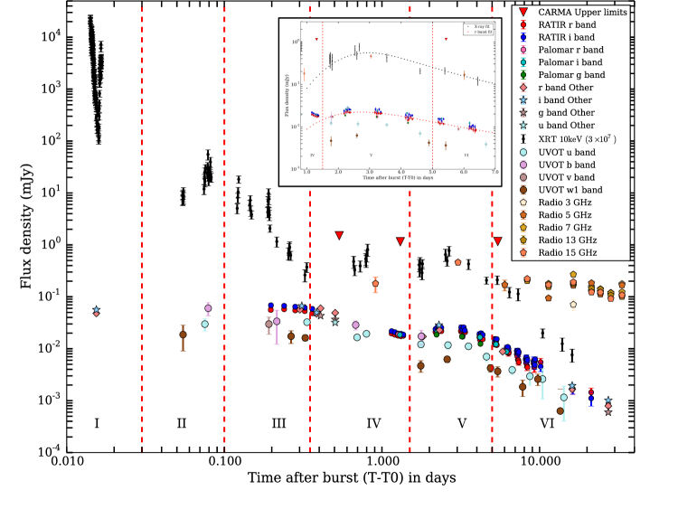
Figure 1: GRB 141121A light curve: we divided the light curve in 6 regions of interest. An achromatic peak is evident at $t\approx 3$ d. In the inset we zoom in this region and over plot to the optical $r^{\prime}$ and X-ray data the best fit for the broken power law (see Table 3).

The X-ray light curve of the afterglow presented in Figure 1 was obtained from the Burst Analyser repository, maintained by the XRT team at the University of Leicester. The light curve, in units of mJy at 10 keV, was extracted using the methods described in Evans et al. (2009, 2010).

Time resolved X-ray spectra of the afterglow in the energy range 0.3–10 keV were extracted for six regions (see later sections). Only grade 0 to 12 events were selected for PC mode data, binning the data in energy with 1 count per bin. xspec v12.8.2 was used for the spectral analysis. An absorbed power-law model was chosen to fit each spectrum, fixing the Galactic absorption to the value in the direction of the GRB of $N_{H}=4.28\times 10^{20}\,{\rm cm}^{-2}$, as calculated from Willingale et al. (2013) and using the TBabs and ZTBabs absorption models at the GRB redshift of $z=1.469$, with the Wilms et al. (2000) abundances. The X-ray fluxes used in the SED analysis, in units of erg cm^-2 s^-1, were derived from the best fit results of the spectral modeling for the six selected time intervals (see Table 3).

The UVOT began settled observations ofGRB 141121A 371 s after the BAT trigger. Initially exposures were taken with all 6 lenticular filters plus the open (white) filter, but after about $T_{BAT}+25$ ks, almost all the exposures used either the u or uvw1 filters, with central wavelengths of 346 nm and 260 nm respectively. Aperture photometry as described by Poole et al. 2008 was carried out for each exposure using the standard HEASOFT 6.16 tools and the latest UVOT calibration (Breeveld et al., 2010, 2011). A 3″ radius aperture was centered on the position determined from the 6 UVOT exposures with the best detections of the afterglow. The measured count rates were corrected for extinction in the Milky Way using the compilation from Schlafly & Finkbeiner (2011) and then converted to fluxes using a standard GRB spectrum (Table 10 in Poole et al., 2008).

2.2 Optical

RATIR started observing GRB 141121A  four hours after the burst and continued monitoring its optical behavior until 21 d post burst, when the afterglow fell below the detection limit of the instrument. The optical camera provided $r^{\prime}$and $i^{\prime}$ observations via a usual sequence consisting of a series of optical frames with exposure times of 80 s each which are reduced in real-time using an automatic pipeline (see Littlejohns et al., 2014, for more details). Multiple exposures were combined in order to increase the signal-to-noise ratio and aperture photometry was performed at the GRB location. Magnitudes were calibrated using nearby point sources from Sloan Digital Sky Survey (SDSS; Ahn et al. 2014).

We imaged the location of GRB 141121A with the robotic Palomar 60-inch telescope (P60; Cenko et al. 2006) beginning at 9:53 UT on 2014 November 22. Observations were obtained in the $g^{\prime}$, $r^{\prime}$, and $i^{\prime}$ filters and continued through 2014 November 27. All data were processed using a custom IRAF pipeline. Individual exposures were aligned with respect to astrometry from the SDSS using SCAMP (Bertin, 2006) and stacked with SWarp (Bertin et al., 2002). We measured aperture photometry on the afterglow of GRB 141121A and used nearby point sources from the SDSS for photometric calibration. The resulting measurements are reported in Table 1.

Finally, further observations were carried out by the Discovery Channel Telescope equipped with the Large Monolithic Imager (LMI) and the Keck I telescope equipped with the Low-resolution Imaging Spectrometer (LRIS, Oke et al., 1995). For LMI, we acquired a series of 2 minutes exposures in $g^{\prime}$,$r^{\prime}$ $i^{\prime}$, and $z^{\prime}$ filters and performed bias subtraction, flat-fielding correction, and cosmic ray removal using our customized pipeline (Toy et al., 2014). A log of all the optical observations is presented in Table 1, after correcting for galactic extinction, assuming $E(B-V)=0.05$ (Schlafly & Finkbeiner, 2011).

2.3 Radio

VLA data were reduced and imaged using the Common Astronomy Software Applications (CASA) package. Specifically, the calibration was performed using the VLA calibration pipeline V4.2.2. After running the pipeline, we inspected the data (calibrators and target source) and applied further flagging when needed. 3C286 was used as flux calibrator. J0830+2410, J0823+2223, and J0802+1809 were used as phase calibrators. The VLA measurement errors are a combination of the rms map error, which measures the contribution of small unresolved fluctuations in the background emission and random map fluctuations due to receiver noise, and a basic fractional error (here estimated to be $\approx 5\%$) which accounts for inaccuracies of the flux density calibration. Theses errors were added in quadrature and total errors are reported in Table 1.

We also observed GRB 141121A  using the Combined Array for Research in Millimeter-wave Astronomy (CARMA) on three occasions between 2014-11-21 UT and 2014-11-26 UT. Observations were conducted in single-polarization mode with the 3 mm receivers tuned to a frequency of 93 GHz, interleaved with observations of a nearby gain-calibrator, as well as observations of 3C84 for flux calibration and 0854+201 for bandpass calibration. Data were reduced using the Multichannel Image Reconstruction Image Analysis Display (MIRIAD) tool; none of the three epochs resulted in a significant detection of the afterglow. A summary of our upper limits is given in Table 1.

2.4 Spectroscopy

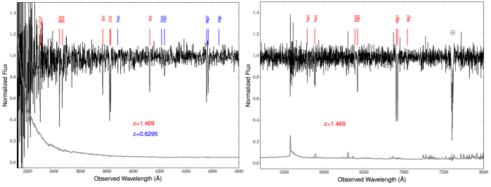
Figure 2: The two panels (separated for simplicity) present two part of the Keck/LRIS spectrum where strong absorption lines belonging to the GRB hosts ($z_{1}=1.469$) and to an intervening system at $z_{2}=0.6295$ appear. We also plot in gray the 1-$\sigma$ error array.

We acquired spectroscopy of the afterglow of GRB 141121A using the Low-Resolution Imaging Spectrograph (LRIS) mounted on the Keck I telescope between 11:10:38 UT and 11:16:18 UT. Observations were taken using the 600/4000 grism on the blue side and 400/8500 grating on the red side, providing continuous wavelength coverage between 3116–10264 Å. Data were reduced in IDL using the LRIS Automated Pipeline (LPipe), with the flux calibration established via a separate observation of the flux standard BD+28. The spectrum (Figure 2) presents several absorption features, including Mg ii doublet (2796,2803Å), Fe ii 2600 and Fe ii 2586 and Fe ii 2344 all at the same redshift of $z=1.4690$. No Ly$\alpha$ line is identified down to the bluer observed wavelengths, providing a stringent upper limit on the GRB redshift of $z<1.56$. We also identify an intervening system at $z=0.6295$, based on Fe ii and Mg ii doublet identification.

2.5 GCN

We complement our data with results obtained by other observatories and published in the GRB Coordinates Network (GCN, Barthelmy et al., 1995). In particular, we use GCN data that complement our light curve observations. For simplicity and to avoid possible cross-calibration issues we used only data obtained in $r^{\prime}$ and $i^{\prime}$ filters (see Table 1 for the relevant references).

3 Analysis

We present in Figure 1 the radio to X-ray light curve of GRB 141121A, and based on the different temporal and spectral behaviors we decided to divide it in six different intervals (I to VI), in order to better study the emission mechanisms in action at each interval. In the standard FS-RS scenario, the afterglow emission is due to synchrotron radiation of shock-accelerated electrons, and we expect the observed spectrum across a large frequency range to be represented by a series of joined power-laws with breaks at characteristic frequencies (Meszaros & Rees, 1997; Sari et al., 1998; Granot & Sari, 2002): a self-absorption frequency ($\nu_{a}$), an injection frequency which identifies the peak of the synchrotron emission ($\nu_{m}$), and the cooling frequency ($\nu_{c}$). The spectral indices ($\beta$) are related to the intrinsic shape of the electron energy distribution (for which a power-law of index $p$ is assumed) and, for a given circumburst medium (ISM or wind, for example), can be related to the temporal indices ($\alpha$) by well-known closure relations (e.g., Racusin, 2009). We report our results for the spectral and temporal indices of GRB 141121A in Table 3. The spectral and temporal behavior of GRB 141121A in regions I to VI can be summarized as follows:

• At $T\lesssim 0.1$ d (regions I and II) the X-ray afterglow shows large flaring activity. The GRB was detected only by the GROND instrument (two hours post-burst) and by UVOT at a flux level ($F_{\rm Opt}=48\mu{\rm Jy}$) which is similar for both regions, suggesting minimal variability.

• In region III ($0.1\,{\rm d}\lesssim T\lesssim 0.35$ d) the X-ray afterglow behaves similarly to the so-called “steep decay phase” (Zhang et al., 2006) observed in other GRBs, with a steep temporal slope ($\alpha_{\rm III,X}=3.1\pm 0.1$, with $\chi^{2}=7.2$ and $d.o.f=9$) and a typical spectral index ($\beta_{X}=0.92\pm 0.17$), despite a hint of flare is present at/around $\sim 2$ d. On the other hand, the optical light curve shows a much shallower decay ($\alpha_{\rm III,Opt}=0.15\pm 0.11$, $\chi^{2}=0.2$ and $d.o.f=2$) and a similar spectral index $\beta_{\rm Opt}=0.87\pm 0.02$. This suggests a different origin for the X-ray and optical emission during this time interval. We interpret the X-ray behavior as a combination of high-latitude emission (Kumar & Panaitescu, 2000) superimposed to some contribution from the original prompt phase, as seen in many other bursts (see for example Nousek et al., 2006; Racusin, 2009; Genet & Granot, 2009, and Section 4 later on). The optical behavior during this time interval (and in regions I and II) is puzzling, and we will discuss possible intepretations in the next sections.

• In region IV ($0.35\,{\rm d}\lesssim T\lesssim 1.5$ d) the optical/UV light curve can be fitted by a single power-law with temporal decay index $\alpha_{\rm IV,Opt}=0.84\pm 0.11$ (standard for afterglow-dominated emission), and spectral index $\beta=0.36\pm 0.21$ (harder than a typical afterglow index). In the X-ray, instead, we see a constant flux, similar to the canonical “plateau” phase (Racusin, 2009), but there is a hint of a possible flare around $T\approx 0.8$ d right at the end of the Swift orbit.

• During region V ($1.5$ d $\lesssim T\lesssim 5$ d), at $\approx 3$ d after the burst, we observe a peak in both the X-ray and optical bands. AMI observations at 14.5 GHz also hint to the presence of a peak around the same time ($\approx 3$ d). We fit the optical and X-ray light curves with a smoothly broken power-law (Beuermann et al., 1999): $F_{\nu}(t)=F_{0}\left[(t/t_{\rm break})^{s\alpha_{\rm rise}}+(t/t_{\rm break})^{s\alpha_{\rm decay}}\right]^{-1/s}$, where we set the roundness parameter to $s=1$. The broken power-law in the X-ray has the following parameters: $\alpha^{\rm rise}_{\rm X}=-2.33\pm 0.88$, $\alpha^{\rm decay}_{\rm X}=2.86\pm 0.21$, $t_{\rm peak}^{\rm X}=3.06\pm 0.71$ d ($\chi^{2}=7.4$ and $d.o.f=8$), while in the optical: $\alpha^{\rm rise}_{\rm Opt}=-1.77\pm 0.77$, $\alpha^{\rm decay}_{\rm Opt}=1.84\pm 0.17$, $t_{\rm peak}^{\rm Opt}=3.53\pm 0.27$ d (with a $\chi^{2}=13.4$ and $d.o.f=29$). A single power law fit does not provide a good representation of such data with a $\chi^{2}=154$ and $d.o.f=28$ (optical) and $\chi^{2}=21$ and $d.o.f=8$ (X-ray). The optical ($\beta_{\rm Opt}=0.78\pm 0.28$) and X-ray ($\beta_{X}=0.67\pm 0.23$) spectral indices show no strong evidence for a spectral break between the two bands within the errors.

• In Region VI (T $\gtrsim 5$ d) we observe a consistent decay, $\alpha_{\rm VI,Opt}=2.06\pm 0.40$ ($\alpha_{\rm VI,X}=2.14\pm 0.34$), in both the X-ray and optical bands ($\chi^{2}=24$ and $d.o.f=21$ and $\chi^{2}=3.7$ and $d.o.f=4$ for the optical and X-ray respectively), and the spectral indices are also consistent within the errors. The radio afterglow at 15 GHz has been monitored since 3 days post bursts and it decays as $\alpha_{15GHz}=0.57\pm 0.10$ until 11 days ($\chi^{2}=2.9$ and $d.o.f=3$). Later observations in the 3-15 GHz range show a flat temporal decay and a soft-to-hard evolution, suggesting a peak sweeping through all the radio frequencies (3-15 GHz; see Table 3 and Section 4).

4 Discussion

A re-brightening similar to the one observed for GRB 141121A  in region V has been observed also in the case of the UL-GRB 111209A (Yu et al., 2013; Stratta et al., 2013). Apart from this GRB, only a few other GRBs, not belonging to the UL-GRB class, present such peculiar feature, but usually at much earlier times ($10^{3}-10^{4}$ s post-burst; e.g. GRB 110213A, GRB 120326A, GRB 120404A Cucchiara et al., 2011; Guidorzi et al., 2014; Melandri et al., 2014; Urata et al., 2014).

Overall, GRB 141121A shares similar characteristics with previously observed UL-GRBs: first, the duration $T=1410$ s which could be due, e.g., to a prolonged central engine activity or to a compact central engine embedded in a large progenitor star (like red supergiant, Quataert & Kasen, 2012; Bromberg et al., 2012, 2011; Woosley & Heger, 2012; Gendre et al., 2013). Second, similarly to GRB 101225A and GRB 111209A, after the prolonged X-ray emission, the light curve rapidly decays (region II). Finally, as pointed out by Levan et al. 2014 (see also GRB 060607A in Ziaeepour et al., 2008), some dips and flaring are sometimes identified after the steep decay phase. Indeed, in the case of GRB 141121A  we see this kind of behavior during region III.

Our extensive follow-up provides a dataset which is ideal to identify the main emission mechanisms (FS, RS, or some combination of both) in action during this burst, and the nature of the surrounding environment (ISM vs. wind). Hereafter, we model the FS and RS synchrotron emission as broken power laws, with breaks at $\nu_{a}<\nu_{m}<\nu_{c}$, with spectral indices $\{-2,-1/3,(p-1)/2,p/2\}$ or $\{-5/2,-2,(p-1)/2,p/2\}$.

As discussed in the previous Section, GRB 141121A shows a very complex light curve. We have identified six different regions with respect to the temporal (and spectral) properties of its afterglow. In what follows, we start our analysis from the latest of these regions (region VI, $T\gtrsim 5$ d), when the afterglow of GRB 141121A seems to settle on a standard power-law decay, and the flaring/re-brightening episodes observed at earlier times seem to be ceased. Then, we discuss the earlier epochs in the light of the constraints derived from region VI.

4.1 Region VI

4.1.1 Evidence for a wind medium

In region VI, the optical and X-ray spectral and temporal indices (see Table 3) are very similar, suggesting that these bands are in the same spectral regime of the synchrotron spectrum predicted by the fireball model. We infer that the most likely scenario is one in which the emission is dominated by a FS with characteristic frequencies $\nu_{m,f}<\nu_{\rm Opt}<\nu_{\rm X}<\nu_{\rm c,f}$. If we parametrize the profile of the circumburst density as $n\propto R^{-k}$, we get (e.g. from Sari & Mészáros, 2000): $k=4/[1+1/(2\alpha_{VI}-3\beta_{VI})]=1.75\pm 0.94$, consistent with a wind environment surrounding the GRB. In this case, the temporal index for the spectral regime $\nu_{m,f}<\nu_{\rm Opt}<\nu_{\rm X}<\nu_{\rm c,f}$ is $\alpha=(1-3p)/4$, from which we estimate $p=2.67\pm 0.08$ for the power-law index of the electron energy distribution. This last result is consistent with the value of $p$ derived from the optical-to-X-ray spectral index $(p-1)/2=\beta_{OX}\approx 0.84\pm 0.02$, which yields $p=2.68\pm 0.05$.

Simple power law fits to the temporal and spectral evolution in this region can be found in Table 3. The model we will introduce in the following sections (Section 4.2.3) gives a good description of this region. Here, the optical and X-ray measurements are the most straightforward to interpret and they can be explained by a simple FS component. Instead, in the radio (in particular at lower frequencies) the RS still dominates.

4.1.2 Source size and scintillation

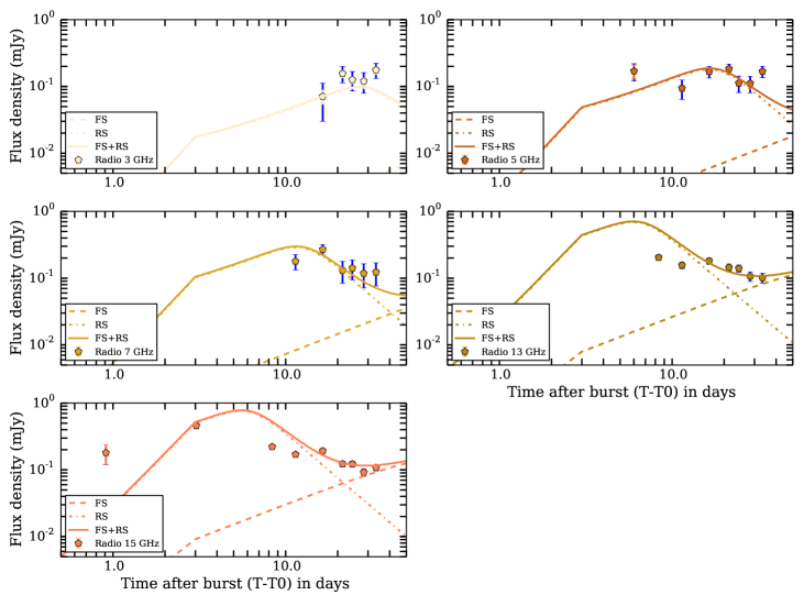
Figure 3: Radio light curves and our model (FS as dashed and RS dotted-dashed) for region VI. We plot with blue errorbars the additional contribution on our error budget from scintillation. While the peak time and the late-time decay ($\alpha\sim 2.0$) is consistent in all the optical/UV bands, the radio flux presents a much shallower decay ($\alpha_{15GHz}\sim 0.57$). Furthermore there is evidence for a peak sweeping through the 3-7 GHz bands between $\approx 10$ d and $\approx 30$ d which we interpret as the passage of $\nu_{SA,f}$. The time evolution of the RS component which on these figures is a power law with two breaks has the following temporal slopes: $\alpha\approx-2.6,-0.86,2.2$. The slope of the FS before and after 3 days is $\alpha\approx-2{\rm~{}and}-1$ respectively.

As evident from the radio late time light curve (Figure 3), the lower-frequency radio data show flux modulations that suggest that interstellar scattering and scintillation (ISS) may be important. At the location of GRB 141121A ($l,b\approx 200^{\circ}$, $27^{\circ}$), the characteristic frequency limiting the strong and weak scattering regime is $\nu_{0}\approx 12$ GHz, and the limiting angular size below which (at this frequency) sources can be considered point sources and exhibit strong scintillation, is $\Theta_{0}\approx 2.5\,\mu{\rm as}$ (Frail et al., 2000).

In the weak scattering regime (in our case, the 14.5 GHz observations) the predicted modulation index can be calculated from (Walker, 1998a, b):

$$m_{\nu}=(\nu/\nu_{0})^{17/12}(\Theta_{\rm source}/\Theta_{F})^{-7/6},$$ (1)

where $\Theta_{F}=\Theta_{0}(\nu/\nu_{0})^{-1/2}$. In the strong scattering regime, the predicted modulation index is:

$$m_{\nu}=(\nu/\nu_{0})^{17/30}(\Theta_{\rm source}/\Theta_{F})^{-7/6},$$ (2)

with $\Theta_{F}=\Theta_{0}(\nu_{0}/\nu)^{11/5}$.

From the data at a given frequency, we estimate the observed modulation index as in (e.g. Cenko et al., 2013; Corsi et al., 2014) :

$$m_{\nu}=\frac{\sqrt{\langle(F_{\nu}-F_{\nu,pred})^{2}\rangle-\langle\sigma_{F_{\nu}}^{2}\rangle}}{\langle F_{\nu}\rangle}$$ (3)

where as predicted flux, $F_{\nu,pred}$, we take a simple power-law fit for every radio band; $\sigma_{F_{\nu}}$ are the measurement errors; and $\langle\dots\rangle$ denotes the average over time. From our VLA observations, we get $m_{3\,{\rm GHz}}\approx 0.3$, $m_{5\,{\rm GHz}}\approx 0.2$, $m_{7\,{\rm GHz}}\approx 0.3$, $m_{13\,{\rm GHz}}\approx 0.1$, $m_{15\,{\rm GHz}}\approx 0.05$. In Figure 3 we show in blue larger error-bars that account for ISS effects.

Using the observed modulation indices (Equation 3) and comparing them with the predicted ones (Equations 1 and 2), we can constrain the apparent size of the emitting region at $\approx 20-25$ d since the burst. The most stringent constraint is derived from the lower frequency observations with the largest modulation indices. The $3$ GHz observation occurs in the strong scattering regime and so we obtain $\Theta_{\rm source}$(20 d)$\approx 76\,\mu{\rm as}$.

We can compare this constraint on the size of the emitting region with the size predicted by the fireball model for a jet expanding in a wind environment (Taylor et al., 2004):

$$\Theta=2R_{\perp}/D_{A}\approx 92\mu{\rm as}~{}({E_{54}}/A_{\star,-2})^{1/4}(t/20\,{\rm d})^{3/4}.$$ (4)

Here, we have expressed the medium density as $n=AR^{-2}$ cm^-3, with $A=3\times 10^{35}A_{\star}$ cm^-1. Thus, if the modulation we observe at the lowest radio frequencies is indeed due to ISS, then $A_{\star}\approx 2.1\times 10^{-2}E_{54}$. This density parameter is quite close to the one derived from modeling in Section 4.2.3.

Finally, because ISS affects more the lower radio frequencies than the higher ones, its effects need to be taken into account when estimating the radio spectral indices. To this end, we compare the spectral indices reported in Table 3 with the ones we obtain from the best fit power-law model that we used to measure the observed modulation indices. At 11 d, the power-law fit gives us $\beta_{radio,pl}\approx-1.5$ (to be compared with the actual value derived from the data of $\beta_{radio}=-1.64\pm 0.32$), at 16 d $\beta_{radio,pl}\approx-0.07$ (to be compared with the actual value derived from the data of $\beta_{radio}=-1.78\pm 0.54$), and at 21 d $\beta_{radio,pl}\approx-0.1$ (to be compared with the actual value derived from the data of $\beta_{radio}=0.18\pm 0.07$). Thus, after correcting for ISS effects, the soft-to-hard evolution observed in the radio band at late times becomes even more evident, supporting the hypothesis of a spectral break passing in band.

4.2 Region V

4.2.1 Deceleration time and initial Lorentz factor

In the fireball model, the afterglow “starts” at the deceleration time, which is related to the location where the jet sweeps up a fraction $1/\Gamma$ of its mass in interstellar material. In a wind case (which, as we have seen in Section 4.1.1, is the most relevant for GRB 141121A), the observed deceleration time is (Zou et al., 2005):

$$t_{\rm dec}=\frac{E(1+z)}{8\pi Am_{p}c^{3}\Gamma_{0}^{4}},$$ (5)

where $\Gamma_{0}$ is the Lorentz factor at the deceleration. Because the power-law behavior observed in region VI extends backwards in time to $\approx 3$ d, we derive $t_{\rm dec}\lesssim 3$ d. Assuming $A_{\star}\approx 0.05$ (as derived in Section 4.2.3), this implies $\Gamma_{0}\gtrsim 27E_{54}^{1/4}(A_{\star}/0.05)^{-1/4}$. This matches with the value of $\Gamma_{0}$ found from modeling in Section 4.2.3.

4.2.2 The peak at 3 d

At $\approx 3$ d, in Region V, a peak (or rebrightening) is observed in the optical and X-ray light curves of GRB 141121A. Because this peak appears to be achromatic (it is observed in both the optical and X-ray, and there are hints of a peak at 15 GHz as well), we consider two scenarios: (i) the peak is marking the deceleration time of the jet whose emission explains region VI data; (ii) this last jet is initially off-axis, and its emission enters our line of sight between 1 d and 3 d post-burst, at which time it peaks at all frequencies.

In Figure 4, we show our extrapolation of the model that explains the optical and X-ray data in region VI, assuming $t_{dec}\approx 3$ d. As evident from Figure 4, because in a wind environment the optical (and X-ray) light curves follow a rather flat temporal behavior, the model overpredicts the optical observations at $t<t_{dec}$. Note also that an earlier deceleration time would make this worse. We thus conclude that the peak observed around 3 d is more easily explained with the off-axis jet hypothesis (ii): in regions V and VI, we are observing emission from a jet (hereafter referred to as the late-time jet) which starts entering our line of sight (and dominating the afterglow emission) in region V. This also implies (as we discuss later on) that the emission observed in regions II-III-IV is likely associated with a second jet (hereafter referred to as the early-time jet), thus favoring a double jet scenario for GRB 141121A . We note that a similar model has been proposed for several GRBs, such as GRB 030329, GRB 120404A, and GRB 080319B (Berger et al., 2003; Guidorzi et al., 2014; Racusin et al., 2008).

The behavior of the radio emission in region V deserves special attention. Extrapolating the late-time X-ray and optical data to the radio band via a simple power-law, overpredicts our radio observations by 2 orders of magnitude. Thus, if the radio peak we observe at 3 d is dominated by FS emission from the late-time jet, then a spectral break between the optical and the radio bands is required. This constrains the location of $\nu_{m,f}$ at $3$ d so that:

$$F_{14.5\rm{GHz}}({\rm 3\,d})=F_{\rm Opt}({\rm 3\,d})\times(\nu_{m,f}/\nu_{\rm Opt})^{-\beta_{\rm OX}}$$ (6)

$$(\nu_{\rm radio}/\nu_{m,f})^{1/3}<0.46\,{\rm mJy}$$

which implies $\nu_{m,f}(3\,\rm{d})>1.2\times 10^{12}$ Hz and $F_{\nu_{m,f}}<2.0$ mJy.

Moreover, if we assume the FS is solely responsible for the radio emission, the low frequency observations at 11 and 16 days need to be consistent with $\nu_{a,f}(\propto t^{-3/5})$ passing through the bands (also with the $21$ d SED where $\nu_{a,f}(21\,{\rm d})<3$ GHz). Accepting these constraints (see also Table 3), we can find the FS self-absorption frequency at 3 d: $\nu_{a,f}({\rm 3\,d})=\nu_{a,f}({\rm 11\,d})(3/11)^{-3/5}\approx 20$ GHz. Using this approximate value for $\nu_{a,f}$ and our conservative lower-limit for $\nu_{m,f}$, we can now give a more quantitative estimate of the FS contribution to the radio flux at 3 d. We have $F_{\rm 14.5GHz}({\rm 3\,d})=F_{\nu_{m,f}}(\nu_{a,f}/\nu_{m,f})^{1/3}(14.5\,{\rm GHz}/\nu_{a,f})^{2}\lesssim 0.2$ mJy. Because the measured flux is $F_{14.5\,\rm GHz}(3\,\rm{d})\approx 0.46$ mJy, this means that at 3 d post burst, at least 50% of the 14.5 GHz flux is provided by a component other that the FS of the late-time jet. We suggest that this component is the RS emission from such jet. We also note that, in fact, if the 15 GHz emission at 3 d was dominated by FS emission at $\nu_{radio}<\nu_{a,f}$, we would expect the emission at $t\gtrsim 3$ d to rise with time as $t^{1}$ until $\nu_{radio}\approx\nu_{a,f}$, and then show a flat behavior ($t^{0}$) until $\nu_{radio}\approx\nu_{m,f}$. This is not what we observe at 15 GHz (see Figure 3).

We model the radio-to-X-ray in a scenario where the optical and X-ray emission are FS-dominated and the 14.5 GHz is RS-dominated. Therefore we can model the SED of GRB 141121A  at 3 d in the same context (Figure  5).In our model presented in Figure 3, we are assuming a deceleration time of 3 d for the late-time jet and we are not attempting modeling the rise before 3 d (since for a jet entering our line of sight, one could have a large range of temporal indices; see e.g. Eichler & Granot 2006).

We finally note that alternative explanations for the $3$ d peak, such as the passing of a characteristic frequency in band, can be excluded. Indeed, the passing of a characteristic frequency in optical or X-rays would imply a chromatic peak time and a spectral evolution across the peak (as seen in other cases; Guidorzi et al., 2014). The optical and X-ray spectral indices of GRB 141121A  before and after the 3 d peak are consistent with no spectral evolution (see Table 3), within the (large) errors, while we do not have spectral information from the radio data around 3 d.

4.2.3 Physical parameters

In order to calculate the physical parameters for this burst, we proceed in the following way: we identify the characteristic frequencies ($\nu_{a}$, $\nu_{m}$ and $\nu_{c}$ for FS and RS) which determine the spectral and temporal evolution of the afterglow. We construct a model using these characteristic frequencies and compare it to our observations. If we find a satisfactory agreement between model and observations, in the next step we solve for the physical parameters that drive the characteristic frequencies.

First, we study the case where the characteristic frequencies have the following ordering: $\nu_{a,f}<\nu_{m,f}<\nu_{c,f}$ and $\nu_{a,r}<\nu_{m,r}<\nu_{c,r}$. We can put a constraint on $\nu_{m,f}$ by requiring the peak flux to lie on the extrapolation of the optical-to-X-ray spectrum below the optical range (e.g. see Equation 6 in Section 4.2.2), $\nu_{c,f}\gtrsim 2.4\times 10^{17}$ Hz and $\nu_{a,f}$ will be unconstrained, because the RS dominates the flux at $\nu_{a,f}$. Similarly in the case of the RS, only $\nu_{m,r}$ can be constrained. We consider the characteristic frequencies $\nu_{m,f}$ and $\nu_{c,f}$ at 3 d as free parameters as well as the total kinetic energy, $E$. Finally, we use the expressions of $\nu_{m,f}$, $\nu_{c,f}$ and $F_{\nu_{m}}$ (e.g. from Granot & Sari, 2002) to determine the efficiencies $\epsilon_{B,f}$, $\epsilon_{e}$ and $A_{\star}$. From the expression of $t_{\rm dec}$ which we equate to $3\,d$ we can derive $\Gamma_{0}$. Using the relations between RS and FS characteristic quantities ($\nu_{m,r}\approx 0.31~{}\Gamma_{0}R_{B}^{1/2}\nu_{m,f}$, $\nu_{c,r}\approx R_{B}^{-3/2}\nu_{c,f}$ and $F_{\nu_{m,r}}\approx 1.2~{}\Gamma_{0}R_{B}^{1/2}F_{\nu_{m,f}}$, where $R_{B}=\epsilon_{B,r}/\epsilon_{B,f}$ e.g. Perley et al. (2014)) we can determine the RS quantities. Here, $R_{B}$ is also a free parameter. We solve the equations for the physical parameters by varying the free parameters ($E$, $\nu_{m,f}$, $\nu_{c,f}$ and $R_{B}$) through the allowed parameter space (or a sufficiently large range in the case of $E$ and $R_{B}$.), we find that either the $\epsilon_{e}<1$ and $\epsilon_{B}<1$ or the $\nu_{a,r}>10$ GHz condition cannot be satisfied at the same time. Violating these conditions makes the solution non-physical, and in particular the latter is important in order for the RS to provide the necessary 15 GHz flux observed at 3 d. We thus conclude that this ordering of the frequencies cannot adequately reproduce the observations.

Next, we assume the RS peak is located at $\nu_{a,r}$, in other words the order of frequencies in the RS is $\nu_{m,r}<\nu_{a,r}<\nu_{c,r}$. We proceed similarly to the previous case: we set up the equations from the expressions of $\nu_{m,f}$, $\nu_{c,f}$, $F_{\nu_{m,f}}$ and $T_{\rm dec}$. Additionally, we consider the expression for $\nu_{a,r}=5.8\times 10^{11}{\rm Hz}~{}(1+z)^{-1}(\epsilon_{e,-0.5}3(p-2)/(p-1))^{6/13}\epsilon_{B,r,-1}^{9/26}E_{54}^{-1}\Gamma_{0,1.5}^{-4}A_{\star,-1}^{43/26}$ (Zou et al., 2005).

We obtain a physically meaningful solution to the set of equations with the following parameters: $\epsilon_{e}=0.405$, $\epsilon_{B,f}=0.023$, $\epsilon_{B,r}=4.1\times 10^{-3}$, $A_{\star}=0.05$ and $\Gamma_{0}=27.2$. We also find a total kinetic energy of $E=10^{54}$ erg, a factor of $\sim 10$ larger than the energy emitted in gamma-rays and a value of $p=2.8$, which is within $2\sigma$ from the value obtained independently from the late time lightcurve. With these parameters, in addition to the model lightcurves, we construct spectral energy distributions for observations after 3 days and show that they provide an adequate description of the data (see Figure 5).

4.3 Regions II-IV

One of the striking features of GRB 141121A is the approximately constant optical flux observed at early times in Region III, with hints of constant flux as early as region I ($\approx 0.01$ d; GROND and UVOT detections). In region IV, before the rebrightening observed in region V, a decaying optical emission is also observed: a second jet component, whose emission dominates at early-times, could explain this unusual behavior. For example, some of the light curves of a two-component jet observed slightly off-axis in Figure 4 of Huang et al. 2004, look qualitatively very similar to the optical light curve of GRB 141121A. We finally note that a two-component jet model with contribution from a RS was also invoked by van der Horst et al. 2014 in the case of GRB 130427A.

5 Conclusions

We have presented our multi-wavelength observing campaign of GRB 141121A , which was discovered by the Swift satellite and observed starting a few hours after the explosion and continuing over the following month. The long duration of this burst places it in the class of UL-GRBs, providing one of the best cases to test the contribution of the RS and its evolution in relation with the FS. Our extensive radio campaign, in combination with the identification of an achromatic peak at $\approx 3$ d, enabled us to demonstrate that the RS is contributing at least 50% of the observed flux, as well as that the complex optical light curve of this burst likely requires a two-component jet model. GRB 141121A is expanding in a wind-like environment, whose density appears to have an average value when compared to the distribution of values observed for other GRBs.

The case of GRB 141121A  shows the importance of combining rapid-response facilities (like RATIR) with Swift as well as with radio observations at various frequencies, overall constraining the temporal behavior of the GRB afterglow over $\sim 10$ orders of magnitude in frequency. UL-GRBs are among the best transient objects for which we can test central engine theories and emission mechanisms, and future planned missions like SVOM (which covers from hard X-ray to optical), XTIDE (designed to observe the transient X-ray sky) or the ISS-Lobster concept will enable great steps forward in our understanding of such phenomena.

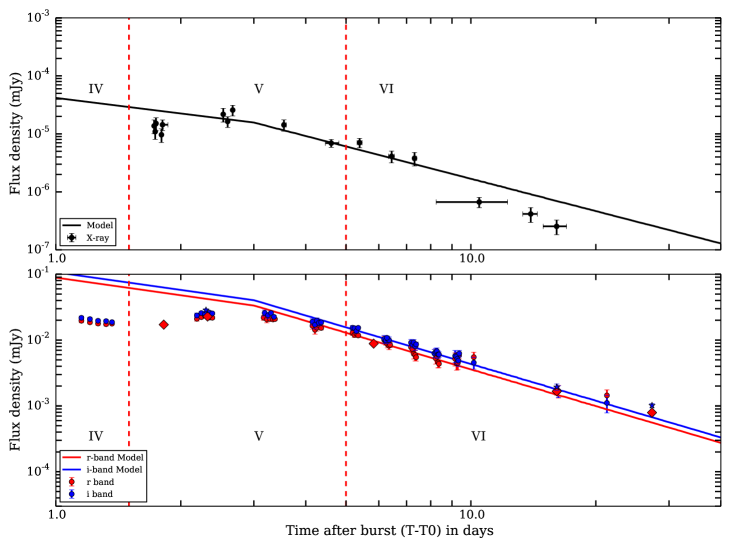
Figure 4: X-ray (top) and Optical (bottom) late-time light curves (including all the data available in the $r^{\prime}$ and $i^{\prime}$ bands). Our model is shown as solid line. The model (see Section 4) describes appropriately the data around and after 3 d.

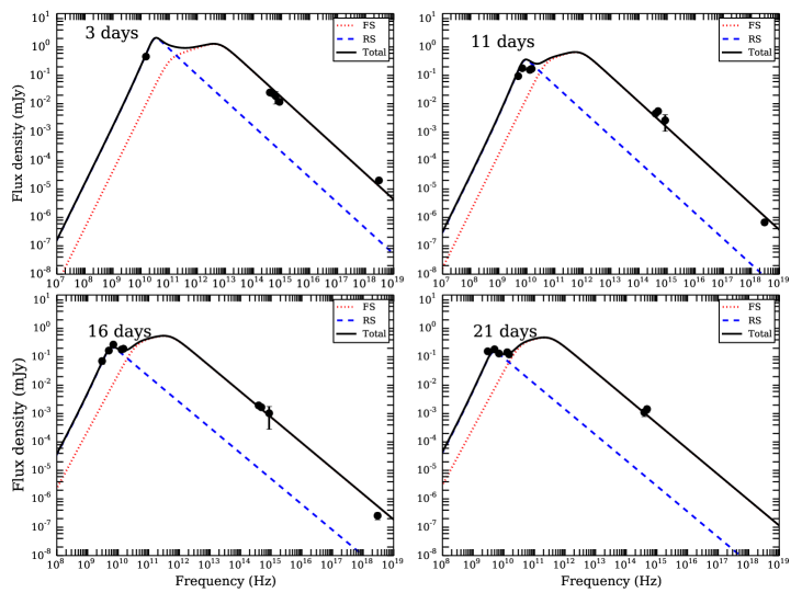
Figure 5: SEDs at 3, 11, 16 and 21 days after the burst: the FS (dashed red), RS (dashed blue) and FS+RS (solid black) contributions to the emission are shown together with the observed radio, optical and X-ray data. The broken power law spectra for both FS and RS represent the standard synchrotron emission expected from a shocked electron distribution (Section 4).

Table 1: Log of Observations

$T-T_{0}$	Mag	Flux	Band	Instrument
(days)		($\mu$Jy)
RATIR
0.197	$19.53\pm 0.08$	$56.05\pm 4.35$	$r^{\prime}$	RATIR
0.239	$19.50\pm 0.07$	$57.62\pm 3.62$	$r^{\prime}$	RATIR
0.282	$19.55\pm 0.07$	$54.79\pm 3.58$	$r^{\prime}$	RATIR
0.324	$19.59\pm 0.07$	$53.15\pm 3.64$	$r^{\prime}$	RATIR
0.361	$19.69\pm 0.07$	$48.28\pm 3.05$	$r^{\prime}$	RATIR
1.152	$20.67\pm 0.07$	$19.67\pm 1.25$	$r^{\prime}$	RATIR
1.208	$20.73\pm 0.07$	$18.61\pm 1.12$	$r^{\prime}$	RATIR
1.264	$20.77\pm 0.07$	$17.84\pm 1.07$	$r^{\prime}$	RATIR
1.321	$20.80\pm 0.06$	$17.43\pm 1.01$	$r^{\prime}$	RATIR
1.365	$20.78\pm 0.04$	$17.77\pm 0.73$	$r^{\prime}$	RATIR
2.186	$20.59\pm 0.09$	$21.08\pm 1.67$	$r^{\prime}$	RATIR
2.241	$20.53\pm 0.06$	$22.33\pm 1.24$	$r^{\prime}$	RATIR
2.287	$20.48\pm 0.06$	$23.40\pm 1.22$	$r^{\prime}$	RATIR
2.346	$20.54\pm 0.06$	$22.04\pm 1.21$	$r^{\prime}$	RATIR
2.382	$20.55\pm 0.04$	$21.84\pm 0.88$	$r^{\prime}$	RATIR
3.167	$20.55\pm 0.09$	$21.90\pm 1.91$	$r^{\prime}$	RATIR
3.223	$20.61\pm 0.12$	$20.62\pm 2.30$	$r^{\prime}$	RATIR
3.279	$20.60\pm 0.08$	$20.93\pm 1.63$	$r^{\prime}$	RATIR
3.336	$20.62\pm 0.07$	$20.59\pm 1.28$	$r^{\prime}$	RATIR
3.371	$20.60\pm 0.05$	$20.83\pm 0.91$	$r^{\prime}$	RATIR
4.151	$20.86\pm 0.12$	$16.50\pm 1.87$	$r^{\prime}$	RATIR
4.210	$21.01\pm 0.15$	$14.35\pm 2.04$	$r^{\prime}$	RATIR
4.252	$20.93\pm 0.12$	$15.49\pm 1.76$	$r^{\prime}$	RATIR
4.302	$20.83\pm 0.10$	$16.90\pm 1.61$	$r^{\prime}$	RATIR
4.357	$20.94\pm 0.07$	$15.28\pm 1.01$	$r^{\prime}$	RATIR
5.187	$21.12\pm 0.09$	$12.91\pm 1.13$	$r^{\prime}$	RATIR
5.242	$21.20\pm 0.09$	$11.99\pm 1.04$	$r^{\prime}$	RATIR
5.296	$21.15\pm 0.08$	$12.59\pm 0.92$	$r^{\prime}$	RATIR
5.351	$21.22\pm 0.06$	$11.76\pm 0.68$	$r^{\prime}$	RATIR
6.182	$21.39\pm 0.14$	$10.07\pm 1.28$	$r^{\prime}$	RATIR
6.237	$21.47\pm 0.11$	$9.35\pm 0.98$	$r^{\prime}$	RATIR
6.292	$21.56\pm 0.12$	$8.61\pm 0.97$	$r^{\prime}$	RATIR
6.350	$21.61\pm 0.14$	$8.22\pm 1.07$	$r^{\prime}$	RATIR
6.385	$21.58\pm 0.10$	$8.47\pm 0.77$	$r^{\prime}$	RATIR
7.172	$21.67\pm 0.14$	$7.79\pm 1.03$	$r^{\prime}$	RATIR
7.228	$21.74\pm 0.13$	$7.30\pm 0.90$	$r^{\prime}$	RATIR
7.283	$21.93\pm 0.17$	$6.16\pm 0.99$	$r^{\prime}$	RATIR
7.339	$21.97\pm 0.20$	$5.94\pm 1.12$	$r^{\prime}$	RATIR
7.379	$22.05\pm 0.14$	$5.48\pm 0.68$	$r^{\prime}$	RATIR
8.167	$21.91\pm 0.16$	$6.26\pm 0.93$	$r^{\prime}$	RATIR
8.223	$22.09\pm 0.20$	$5.29\pm 0.97$	$r^{\prime}$	RATIR
8.279	$22.02\pm 0.17$	$5.63\pm 0.87$	$r^{\prime}$	RATIR
8.336	$22.25\pm 0.19$	$4.58\pm 0.80$	$r^{\prime}$	RATIR
8.371	$22.30\pm 0.14$	$4.37\pm 0.57$	$r^{\prime}$	RATIR
9.161	$22.11\pm 0.24$	$5.20\pm 1.16$	$r^{\prime}$	RATIR
9.236	$22.28\pm 0.24$	$4.45\pm 0.98$	$r^{\prime}$	RATIR
9.298	$22.27\pm 0.23$	$4.49\pm 0.95$	$r^{\prime}$	RATIR
9.362	$21.98\pm 0.13$	$5.86\pm 0.68$	$r^{\prime}$	RATIR
10.158	$22.05\pm 0.20$	$5.50\pm 1.02$	$r^{\prime}$	RATIR
16.245	$23.33\pm 0.23$	$1.68\pm 0.36$	$r^{\prime}$	RATIR
21.261	$23.50\pm 0.23$	$1.44\pm 0.31$	$r^{\prime}$	RATIR
0.198	$19.31\pm 0.08$	$68.60\pm 4.75$	$i^{\prime}$	RATIR
0.239	$19.33\pm 0.07$	$67.05\pm 4.02$	$i^{\prime}$	RATIR
0.282	$19.38\pm 0.07$	$64.41\pm 3.97$	$i^{\prime}$	RATIR
0.324	$19.43\pm 0.07$	$61.54\pm 3.93$	$i^{\prime}$	RATIR
0.361	$19.48\pm 0.06$	$58.50\pm 3.21$	$i^{\prime}$	RATIR
1.152	$20.56\pm 0.07$	$21.77\pm 1.40$	$i^{\prime}$	RATIR
1.208	$20.60\pm 0.06$	$20.82\pm 1.23$	$i^{\prime}$	RATIR
1.264	$20.67\pm 0.06$	$19.63\pm 1.14$	$i^{\prime}$	RATIR
1.321	$20.68\pm 0.06$	$19.39\pm 1.15$	$i^{\prime}$	RATIR
1.365	$20.72\pm 0.05$	$18.72\pm 0.78$	$i^{\prime}$	RATIR
2.186	$20.46\pm 0.09$	$23.72\pm 1.98$	$i^{\prime}$	RATIR
2.241	$20.37\pm 0.06$	$25.72\pm 1.46$	$i^{\prime}$	RATIR
2.287	$20.40\pm 0.06$	$25.02\pm 1.40$	$i^{\prime}$	RATIR
2.346	$20.36\pm 0.06$	$26.08\pm 1.41$	$i^{\prime}$	RATIR
2.382	$20.39\pm 0.04$	$25.43\pm 1.03$	$i^{\prime}$	RATIR
3.184	$20.37\pm 0.11$	$25.83\pm 2.66$	$i^{\prime}$	RATIR
3.243	$20.46\pm 0.12$	$23.72\pm 2.61$	$i^{\prime}$	RATIR
3.298	$20.37\pm 0.08$	$25.76\pm 1.81$	$i^{\prime}$	RATIR
3.353	$20.52\pm 0.05$	$22.54\pm 1.03$	$i^{\prime}$	RATIR
4.151	$20.71\pm 0.12$	$18.95\pm 2.10$	$i^{\prime}$	RATIR
4.210	$20.82\pm 0.14$	$17.07\pm 2.14$	$i^{\prime}$	RATIR
4.252	$20.66\pm 0.10$	$19.81\pm 1.92$	$i^{\prime}$	RATIR
4.302	$20.75\pm 0.11$	$18.24\pm 1.78$	$i^{\prime}$	RATIR
4.357	$20.73\pm 0.07$	$18.57\pm 1.14$	$i^{\prime}$	RATIR
5.187	$20.93\pm 0.09$	$15.39\pm 1.23$	$i^{\prime}$	RATIR
5.242	$20.95\pm 0.08$	$15.11\pm 1.17$	$i^{\prime}$	RATIR
5.296	$21.06\pm 0.08$	$13.73\pm 1.04$	$i^{\prime}$	RATIR
5.351	$20.94\pm 0.06$	$15.34\pm 0.80$	$i^{\prime}$	RATIR
6.182	$21.36\pm 0.14$	$10.37\pm 1.37$	$i^{\prime}$	RATIR
6.237	$21.41\pm 0.11$	$9.87\pm 0.96$	$i^{\prime}$	RATIR
6.292	$21.35\pm 0.11$	$10.49\pm 1.04$	$i^{\prime}$	RATIR
6.350	$21.40\pm 0.13$	$9.99\pm 1.16$	$i^{\prime}$	RATIR
6.275	$21.31\pm 0.04$	$10.82\pm 0.44$	$i^{\prime}$	RATIR
7.172	$21.50\pm 0.13$	$9.14\pm 1.07$	$i^{\prime}$	RATIR
7.228	$21.58\pm 0.12$	$8.49\pm 0.97$	$i^{\prime}$	RATIR
7.283	$21.49\pm 0.12$	$9.21\pm 0.98$	$i^{\prime}$	RATIR
7.339	$21.64\pm 0.15$	$8.03\pm 1.09$	$i^{\prime}$	RATIR
7.379	$21.56\pm 0.09$	$8.60\pm 0.71$	$i^{\prime}$	RATIR
8.167	$21.91\pm 0.15$	$6.28\pm 0.89$	$i^{\prime}$	RATIR
8.223	$21.85\pm 0.14$	$6.62\pm 0.86$	$i^{\prime}$	RATIR
8.279	$21.82\pm 0.13$	$6.78\pm 0.82$	$i^{\prime}$	RATIR
8.336	$21.95\pm 0.14$	$6.05\pm 0.80$	$i^{\prime}$	RATIR
8.371	$21.95\pm 0.11$	$6.04\pm 0.58$	$i^{\prime}$	RATIR
9.161	$22.00\pm 0.23$	$5.74\pm 1.21$	$i^{\prime}$	RATIR
9.216	$22.03\pm 0.19$	$5.62\pm 0.99$	$i^{\prime}$	RATIR
9.271	$22.12\pm 0.18$	$5.17\pm 0.88$	$i^{\prime}$	RATIR
9.326	$22.18\pm 0.20$	$4.88\pm 0.89$	$i^{\prime}$	RATIR
9.371	$21.91\pm 0.12$	$6.26\pm 0.70$	$i^{\prime}$	RATIR
10.158	$22.26\pm 0.22$	$4.54\pm 0.92$	$i^{\prime}$	RATIR
16.245	$23.34\pm 0.22$	$1.68\pm 0.35$	$i^{\prime}$	RATIR
21.261	$23.79\pm 0.32$	$1.11\pm 0.33$	$i^{\prime}$	RATIR
Palomar P60
1.270	$20.70\pm 0.03$	$19.02\pm 0.51$	$r^{\prime}$	Palomar-P60
2.250	$20.57\pm 0.08$	$21.40\pm 1.50$	$r^{\prime}$	Palomar-P60
3.250	$20.80\pm 0.09$	$17.44\pm 1.51$	$r^{\prime}$	Palomar-P60
4.170	$20.82\pm 0.06$	$17.05\pm 0.93$	$r^{\prime}$	Palomar-P60
5.300	$21.16\pm 0.07$	$12.49\pm 0.83$	$r^{\prime}$	Palomar-P60
6.160	$21.52\pm 0.10$	$8.97\pm 0.78$	$r^{\prime}$	Palomar-P60
1.300	$20.68\pm 0.04$	$18.55\pm 0.62$	$i^{\prime}$	Palomar-P60
2.240	$20.37\pm 0.07$	$20.87\pm 1.37$	$i^{\prime}$	Palomar-P60
3.240	$20.45\pm 0.09$	$17.01\pm 1.35$	$i^{\prime}$	Palomar-P60
4.190	$20.59\pm 0.05$	$16.63\pm 0.74$	$i^{\prime}$	Palomar-P60
5.290	$20.91\pm 0.07$	$12.18\pm 0.75$	$i^{\prime}$	Palomar-P60
6.180	$21.17\pm 0.08$	$8.75\pm 0.68$	$i^{\prime}$	Palomar-P60
2.220	$20.72\pm 0.05$	$18.67\pm 0.89$	$g^{\prime}$	Palomar-P60
3.220	$20.81\pm 0.06$	$17.17\pm 0.92$	$g^{\prime}$	Palomar-P60
4.220	$21.17\pm 0.05$	$12.41\pm 0.55$	$g^{\prime}$	Palomar-P60
Discovery Channel Telescope
16.098	$23.34\pm 0.14$	$1.67\pm 0.21$	$r^{\prime}$	DCT
16.098	$23.18\pm 0.12$	$1.94\pm 0.21$	$i^{\prime}$	DCT
UVOT
0.075	$20.21\pm 0.29$	$29.79\pm 7.85$	u	UVOT
0.335	$20.12\pm 0.11$	$32.48\pm 3.38$	u	UVOT
0.695	$20.86\pm 0.09$	$16.52\pm 1.42$	u	UVOT
0.797	$20.68\pm 0.11$	$19.39\pm 1.91$	u	UVOT
1.768	$21.19\pm 0.14$	$12.12\pm 1.62$	u	UVOT
2.624	$21.23\pm 0.18$	$11.70\pm 1.97$	u	UVOT
3.541	$21.28\pm 0.13$	$11.13\pm 1.34$	u	UVOT
4.607	$21.78\pm 0.22$	$7.02\pm 1.40$	u	UVOT
6.705	$22.42\pm 0.20$	$3.90\pm 0.72$	u	UVOT
8.683	$22.73\pm 0.36$	$2.95\pm 0.98$	u	UVOT
10.448	$22.86\pm 0.64$	$2.61\pm 1.53$	u	UVOT
14.266	$23.75\pm 0.71$	$1.15\pm 0.75$	u	UVOT
0.079	$19.45\pm 0.31$	$60.20\pm 17.24$	b	UVOT
0.215	$20.08\pm 0.69$	$33.67\pm 21.49$	b	UVOT
0.681	$20.26\pm 0.22$	$28.66\pm 5.73$	b	UVOT
1.777	$20.80\pm 0.33$	$17.33\pm 5.32$	b	UVOT
0.192	$20.21\pm 0.40$	$29.81\pm 10.85$	v	UVOT
0.055	$20.72\pm 0.56$	$18.73\pm 9.66$	uvw1	UVOT
0.265	$20.80\pm 0.30$	$17.40\pm 4.77$	uvw1	UVOT
0.326	$20.88\pm 0.14$	$16.17\pm 2.03$	uvw1	UVOT
1.764	$22.22\pm 0.27$	$4.70\pm 1.18$	uvw1	UVOT
2.593	$21.91\pm 0.14$	$6.26\pm 0.82$	uvw1	UVOT
4.884	$22.33\pm 0.18$	$4.23\pm 0.70$	uvw1	UVOT
5.424	$22.49\pm 0.24$	$3.67\pm 0.83$	uvw1	UVOT
7.812	$23.24\pm 0.38$	$1.84\pm 0.65$	uvw1	UVOT
9.751	$22.86\pm 0.27$	$2.60\pm 0.64$	uvw1	UVOT
13.531	$24.40\pm 1.78$	$0.63\pm 1.04$	uvw1	UVOT
GCN
0.505	$20.13\pm 0.08$	$32.06\pm 2.36$	$u^{\prime}$	Keck-LRIS
0.408	$19.81\pm 0.01$	$43.33\pm 0.40$	$g^{\prime}$	Keck-LRIS
0.505	$19.99\pm 0.02$	$36.71\pm 0.68$	$g^{\prime}$	Keck-LRIS
27.305	$24.46\pm 0.04$	$0.60\pm 0.02$	$g^{\prime}$	Keck-LRIS
0.015	$19.70\pm 0.10$	$48.09\pm 4.43$	$g^{\prime}$	GROND1
0.302	$19.52\pm 0.06$	$56.76\pm 3.14$	$r^{\prime}$	LCO-FTN2
0.385	$19.71\pm 0.10$	$47.21\pm 4.35$	$r^{\prime}$	MITSuME3
0.408	$19.45\pm 0.01$	$59.98\pm 0.55$	$r^{\prime}$	Keck-LRIS
0.505	$19.68\pm 0.02$	$48.98\pm 0.90$	$r^{\prime}$	Keck-LRIS
1.819	$20.82\pm 0.03$	$17.14\pm 0.47$	$r^{\prime}$	TSHAO4
2.320	$20.50\pm 0.04$	$22.80\pm 0.84$	$r^{\prime}$	LCO-FTN2
5.830	$21.54\pm 0.09$	$8.83\pm 0.73$	$r^{\prime}$	TSHAO6
27.305	$24.16\pm 0.09$	$0.79\pm 0.07$	$r^{\prime}$	Keck-LRIS
0.015	$19.52\pm 0.10$	$56.39\pm 5.19$	$i^{\prime}$	GROND1
0.310	$19.34\pm 0.06$	$66.56\pm 3.68$	$i^{\prime}$	LCO-FTN2
0.385	$19.66\pm 0.10$	$49.57\pm 4.57$	$i^{\prime}$	MITSuME3
2.300	$20.26\pm 0.05$	$28.53\pm 1.31$	$i^{\prime}$	LCO-FTN2
27.305	$23.88\pm 0.07$	$1.02\pm 0.07$	$i^{\prime}$	Keck-LRIS

Note. — Magnitude presented are corrected for galactic extinction using Schlafly & Finkbeiner (2011)

Note. — References: (1)Tanga et al. (2014); (2) Dichiara & Guidorzi (2014a); Kurita et al. (2014); (4)Volnova et al. (2014); (5)Dichiara & Guidorzi (2014b); (6)Mazaeva et al. (2014)

Table 2: Log of Radio Observations

$T-T_{0}$	Flux	Band	Instrument
(days)	($\mu$Jy)
0.536	$\lesssim 1500$	93 GHz	CARMA
0.910	$180\pm 60$	15 GHz	AMI-LA
1.308	$\lesssim 1150$	93 GHz	CARMA
3.037	$460\pm 50$	15 GHz	AMI-LA
5.433	$\lesssim 1160$	93 GHz	CARMA
6.016	$170\pm 40$	4.9 GHz	WSRT
8.352	$204\pm 12$	13 GHz	VLA
8.352	$222\pm 13$	15 GHz	VLA
11.402	$170\pm 11$	15 GHz	VLA
11.402	$94.0\pm 9.8$	5 GHz	VLA
11.402	$179\pm 12$	7 GHz	VLA
11.402	$156\pm 10$	13 GHz	VLA
16.385	$71\pm 17$	3 GHz	VLA
16.385	$166\pm 15$	5 GHz	VLA
16.385	$270\pm 18$	7 GHz	VLA
16.385	$181\pm 13$	13 GHz	VLA
16.385	$192\pm 14$	15 GHz	VLA
21.350	$156\pm 21$	3 GHz	VLA
21.350	$184\pm 15$	5 GHz	VLA
21.350	$131\pm 15$	7 GHz	VLA
21.350	$144.9\pm 9.4$	13 GHz	VLA
21.350	$122.0\pm 8.7$	15 GHz	VLA
24.329	$126\pm 17$	3 GHz	VLA
24.329	$112\pm 11$	5 GHz	VLA
24.329	$141\pm 14$	7 GHz	VLA
24.329	$140\pm 9$	13 GHz	VLA
24.329	$122\pm 9$	15 GHz	VLA
28.323	$120\pm 17$	3 GHz	VLA
28.323	$111\pm 11$	5 GHz	VLA
28.323	$118\pm 12$	7 GHz	VLA
28.323	$106.7\pm 8.1$	13 GHz	VLA
28.323	$92.0\pm 7.8$	15 GHz	VLA
33.350	$177\pm 25$	3 GHz	VLA
33.350	$168\pm 15$	5 GHz	VLA
33.350	$123\pm 13$	7 GHz	VLA
33.350	$101.0\pm 8.7$	13 GHz	VLA
33.350	$108\pm 7$	15 GHz	VLA

Note. — Radio observations obtained with the VLA and CARMA facilities. We also list some publicly available data obtained with the AMI-LA telescope (Anderson et al., 2014) and WSRT (van der Horst, 2014).

Table 3: Spectral analysis

Region	Temporal	Spectral
	index	index
Region I	…	$\beta_{Opt}=0.74\pm 0.47$
	…	$\beta_{X}=0.55\pm 0.04$
Region II	…	$\beta_{Opt}=3.3\pm 0.17$
	…	$\beta_{X}=0.92\pm 0.17$
Region III	$\alpha_{Opt}=0.15\pm 0.11$	$\beta_{Opt}=0.87\pm 0.14$
	$\alpha_{X}=3.17\pm 0.14$	$\beta_{X}=0.92\pm 0.13$
Region IV	$\alpha_{Opt}=0.84\pm 0.11$	$\beta_{Opt}=0.29\pm 0.21$
	…	$\beta_{X}=0.83\pm 0.21$
Region V	$\alpha_{Opt}^{rise}=-1.77\pm 0.77$	$\beta_{Opt}^{rise}=0.49\pm 0.18$
	$\alpha_{Opt}^{decay}=1.84\pm 0.17$	$\beta_{Opt}^{decay}=0.83\pm 0.16$
	$\alpha_{X}^{rise}=-2.33\pm 0.88$	$\beta_{X}=0.67\pm 0.23$
	$\alpha_{X}^{decay}=2.86\pm 0.21$
Region VI	$\alpha_{Opt}=1.65\pm 0.40$	$\beta_{Opt}=0.84\pm 0.47$
	$\alpha_{X}=1.85\pm 0.34$	$\beta_{X}=0.86\pm 0.33$
	$\alpha_{3GHz}=-0.87\pm 0.32$	$\beta_{radio}(11\,{\rm d)}=-0.34\pm 0.05$
	$\alpha_{5GHz}=-0.19\pm 0.10$	$\beta_{radio}(16\,{\rm d)}=-0.16\pm 0.06$
	$\alpha_{7GHz}=0.45\pm 0.09$	$\beta_{radio}(21\,{\rm d)}=+0.18\pm 0.07$
	$\alpha_{13GHz}=0.43\pm 0.05$	$\beta_{radio}(25\,{\rm d)}=-0.06\pm 0.07$
	$\alpha_{15GHz}=0.57\pm 0.05$	$\beta_{radio}(28\,{\rm d)}=+0.12\pm 0.06$
	…	$\beta_{radio}(33\,{\rm d)}=+0.37\pm 0.08$

Note. — Temporal and spectral analysis results for the different regions. In regions I and II the temporal indices in optical and X-ray are not calculated because of lack of measurements (optical) or rapid variation within the same region (X-ray). See the main text for more details.

References

- Ahn et al. (2014) Ahn, C. P., Alexandroff, R., Allende Prieto, C., et al. 2014, ApJS, 211, 17
- Akerlof et al. (1999) Akerlof, C., Balsano, R., Barthelmy, S., et al. 1999, Nature, 398, 400
- Anderson et al. (2014) Anderson, G. E., Fender, R. P., & Staley, T. D. 2014, GRB Coordinates Network, 17099, 1
- Barthelmy et al. (1995) Barthelmy, S. D., Butterworth, P., Cline, T. L., et al. 1995, Ap&SS, 231, 235
- Barthelmy et al. (2005) Barthelmy, S. D., Barbier, L. M., Cummings, J. R., et al. 2005, Space Science Reviews, 120, 143
- Berger (2014) Berger, E. 2014, ARA&A, 52, 43
- Berger et al. (2003) Berger, E., Kulkarni, S. R., Pooley, G., et al. 2003, Nature, 426, 154
- Bertin (2006) Bertin, E. 2006, in Astronomical Society of the Pacific Conference Series, Vol. 351, Astronomical Data Analysis Software and Systems XV, ed. C. Gabriel, C. Arviset, D. Ponz, & S. Enrique, 112
- Bertin et al. (2002) Bertin, E., Mellier, Y., Radovich, M., et al. 2002, in Astronomical Society of the Pacific Conference Series, Vol. 281, Astronomical Data Analysis Software and Systems XI, ed. D. A. Bohlender, D. Durand, & T. H. Handley, 228
- Beuermann et al. (1999) Beuermann, K., Hessman, F. V., Reinsch, K., et al. 1999, A&A, 352, L26
- Bloom et al. (2011) Bloom, J. S., Giannios, D., Metzger, B. D., et al. 2011, Science, 333, 203
- Breeveld et al. (2011) Breeveld, A. A., Landsman, W., Holland, S. T., et al. 2011, in American Institute of Physics Conference Series, Vol. 1358, American Institute of Physics Conference Series, ed. J. E. McEnery, J. L. Racusin, & N. Gehrels, 373–376
- Breeveld et al. (2010) Breeveld, A. A., Curran, P. A., Hoversten, E. A., et al. 2010, MNRAS, 406, 1687
- Bromberg et al. (2011) Bromberg, O., Nakar, E., Piran, T., & Sari, R. 2011, ApJ, 740, 100
- Bromberg et al. (2012) —. 2012, ApJ, 749, 110
- Burrows et al. (2005) Burrows, D. N., Hill, J. E., Nousek, J. A., et al. 2005, Space Science Reviews, 120, 165
- Butler et al. (2012) Butler, N., Klein, C., Fox, O., et al. 2012, in Society of Photo-Optical Instrumentation Engineers (SPIE) Conference Series, Vol. 8446, Society of Photo-Optical Instrumentation Engineers (SPIE) Conference Series, 10
- Cenko et al. (2006) Cenko, S. B., Fox, D. B., Moon, D.-S., et al. 2006, PASP, 118, 1396
- Cenko et al. (2013) Cenko, S. B., Kulkarni, S. R., Horesh, A., et al. 2013, ApJ, 769, 130
- Corsi et al. (2014) Corsi, A., Ofek, E. O., Gal-Yam, A., et al. 2014, ApJ, 782, 42
- Cucchiara et al. (2011) Cucchiara, A., Cenko, S. B., Bloom, J. S., et al. 2011, ApJ, 743, 154
- Dichiara & Guidorzi (2014a) Dichiara, S., & Guidorzi, C. 2014a, GRB Coordinates Network
- Dichiara & Guidorzi (2014b) —. 2014b, GRB Coordinates Network
- Eichler & Granot (2006) Eichler, D., & Granot, J. 2006, ApJ, 641, L5
- Evans et al. (2007) Evans, P. A., Beardmore, A. P., Page, K. L., et al. 2007, A&A, 469, 379
- Evans et al. (2009) —. 2009, MNRAS, 397, 1177
- Evans et al. (2010) Evans, P. A., Willingale, R., Osborne, J. P., et al. 2010, A&A, 519, A102
- Evans et al. (2014) —. 2014, MNRAS, 444, 250
- Frail et al. (2000) Frail, D. A., Kulkarni, S. R., Sari, R., et al. 2000, ApJ, 534, 559
- Gal-Yam et al. (2006) Gal-Yam, A., Fox, D. B., Price, P. A., et al. 2006, Nature, 444, 1053
- Gehrels et al. (2004) Gehrels, N., Chincarini, G., Giommi, P., et al. 2004, ApJ, 611, 1005
- Gendre et al. (2012) Gendre, B., Atteia, J. L., Boër, M., et al. 2012, ApJ, 748, 59
- Gendre et al. (2013) Gendre, B., Stratta, G., Atteia, J. L., et al. 2013, ApJ, 766, 30
- Genet & Granot (2009) Genet, F., & Granot, J. 2009, MNRAS, 399, 1328
- Golenetskii et al. (2014) Golenetskii, S., Aptekar, R. L., & Frederiks, D. D. 2014, GRB Coordinates Network
- Granot & Sari (2002) Granot, J., & Sari, R. 2002, ApJ, 568, 820
- Guidorzi et al. (2014) Guidorzi, C., Mundell, C. G., Harrison, R., et al. 2014, MNRAS, 438, 752
- Honda et al. (2014) Honda, F., Fukushima, K., Negoro, H., et al. 2014, GRB Coordinates Network, 17077, 1
- Huang et al. (2004) Huang, Y. F., Wu, X. F., Dai, Z. G., Ma, H. T., & Lu, T. 2004, ApJ, 605, 300
- Kobayashi & Zhang (2003) Kobayashi, S., & Zhang, B. 2003, ApJ, 597, 455
- Kouveliotou et al. (1993) Kouveliotou, C., Meegan, C. A., Fishman, G. J., et al. 1993, ApJ, 413, L101
- Kulkarni et al. (1999) Kulkarni, S. R., Djorgovski, S. G., Odewahn, S. C., et al. 1999, Nature, 398, 389
- Kumar & Panaitescu (2000) Kumar, P., & Panaitescu, A. 2000, ApJ, 541, L51
- Kurita et al. (2014) Kurita, S., Saito, Y., & Tachibana, Y. 2014, GRB Coordinates Network
- Laskar et al. (2013) Laskar, T., Berger, E., Zauderer, B. A., et al. 2013, ApJ, 776, 119
- Levan et al. (2014) Levan, A. J., Tanvir, N. R., Starling, R. L. C., et al. 2014, ApJ, 781, 13
- Lien et al. (2014) Lien, A. Y., Kennea, J. A., & Krimm, H. A. 2014, GRB Coordinates Network, 17078, 1
- Littlejohns et al. (2014) Littlejohns, O. M., Butler, N. R., Cucchiara, A., et al. 2014, AJ, 148, 2
- Mazaeva et al. (2014) Mazaeva, E., Kusakin, A., & Volnova, A. 2014, GRB Coordinates Network
- Melandri et al. (2008) Melandri, A., Mundell, C. G., Kobayashi, S., et al. 2008, ApJ, 686, 1209
- Melandri et al. (2014) Melandri, A., Virgili, F. J., Guidorzi, C., et al. 2014, A&A, 572, A55
- Meszaros & Rees (1993) Meszaros, P., & Rees, M. J. 1993, ApJ, 418, L59+
- Meszaros & Rees (1997) —. 1997, ApJ, 476, 232
- Mészáros & Rees (1999) Mészáros, P., & Rees, M. J. 1999, MNRAS, 306, L39
- Nousek et al. (2006) Nousek, J. A., Kouveliotou, C., Grupe, D., et al. 2006, ApJ, 642, 389
- Oke et al. (1995) Oke, J. B., Cohen, J. G., Carr, M., et al. 1995, PASP, 107, 375
- Perley et al. (2014) Perley, D. A., Cenko, S. B., Corsi, A., et al. 2014, ApJ, 781, 37
- Perley et al. (2009) Perley, R., Napier, P., Jackson, J., et al. 2009, IEEE Proceedings, 97, 1448
- Piro et al. (2014) Piro, L., Troja, E., Gendre, B., et al. 2014, ApJ, 790, L15
- Poole et al. (2008) Poole, T. S., Breeveld, A. A., Page, M. J., et al. 2008, MNRAS, 383, 627
- Quataert & Kasen (2012) Quataert, E., & Kasen, D. 2012, MNRAS, 419, L1
- Racusin (2009) Racusin, J. L. 2009, PhD thesis, The Pennsylvania State University
- Racusin et al. (2008) Racusin, J. L., Karpov, S. V., Sokolowski, M., et al. 2008, Nature, 455, 183
- Roming et al. (2005) Roming, P. W. A., Kennedy, T. E., Mason, K. O., et al. 2005, Space Science Reviews, 120, 95
- Sakamoto et al. (2011) Sakamoto, T., Barthelmy, S. D., Baumgartner, W. H., et al. 2011, ApJS, 195, 2
- Sari & Mészáros (2000) Sari, R., & Mészáros, P. 2000, ApJ, 535, L33
- Sari & Piran (1999) Sari, R., & Piran, T. 1999, ApJ, 517, L109
- Sari et al. (1998) Sari, R., Piran, T., & Narayan, R. 1998, ApJ, 497, L17+
- Schlafly & Finkbeiner (2011) Schlafly, E. F., & Finkbeiner, D. P. 2011, ApJ, 737, 103
- Soderberg et al. (2006) Soderberg, A. M., Kulkarni, S. R., Nakar, E., et al. 2006, Nature, 442, 1014
- Stratta et al. (2013) Stratta, G., Gendre, B., Atteia, J. L., et al. 2013, ApJ, 779, 66
- Tanga et al. (2014) Tanga, M., Kann, D. A., & Greiner, J. 2014, GRB Coordinates Network, 17078, 1
- Tanvir et al. (2013) Tanvir, N. R., Levan, A. J., Fruchter, A. S., et al. 2013, Nature, 500, 547
- Tanvir et al. (2009) Tanvir, N. R., Fox, D. B., Levan, A. J., et al. 2009, Nature, 461, 1254
- Taylor et al. (2004) Taylor, G. B., Frail, D. A., Berger, E., & Kulkarni, S. R. 2004, ApJ, 609, L1
- Toy et al. (2014) Toy, V., Capone, J., & Cucchiara, A. 2014, GRB Coordinates Network
- Urata et al. (2014) Urata, Y., Huang, K., Takahashi, S., et al. 2014, ApJ, 789, 146
- van der Horst (2014) van der Horst, A. J. 2014, GRB Coordinates Network, 17104, 1
- van der Horst et al. (2014) van der Horst, A. J., Paragi, Z., de Bruyn, A. G., et al. 2014, MNRAS, 444, 3151
- Veres et al. (2014) Veres, P., Corsi, A., Frail, D. A., Cenko, S. B., & Perley, D. A. 2014, ArXiv e-prints, arXiv:1411.7368
- Vestrand et al. (2014) Vestrand, W. T., Wren, J. A., Panaitescu, A., et al. 2014, Science, 343, 38
- Virgili et al. (2013) Virgili, F. J., Mundell, C. G., Pal’shin, V., et al. 2013, ApJ, 778, 54
- Volnova et al. (2014) Volnova, A., Reva, I., & Kusakin, A. 2014, GRB Coordinates Network
- Walker (1998a) Walker, M. A. 1998a, MNRAS, 294, 307
- Walker (1998b) —. 1998b, MNRAS, 294, 307
- Willingale et al. (2013) Willingale, R., Starling, R. L. C., Beardmore, A. P., Tanvir, N. R., & O’Brien, P. T. 2013, MNRAS, 431, 394
- Wilms et al. (2000) Wilms, J., Allen, A., & McCray, R. 2000, ApJ, 542, 914
- Woosley & Bloom (2006) Woosley, S. E., & Bloom, J. S. 2006, ARA&A, 44, 507
- Woosley & Heger (2012) Woosley, S. E., & Heger, A. 2012, ApJ, 752, 32
- Yu et al. (2013) Yu, Y. B., Wu, X. F., Huang, Y. F., et al. 2013, ArXiv e-prints, arXiv:1312.0794
- Zhang et al. (2006) Zhang, B., Fan, Y. Z., Dyks, J., et al. 2006, ApJ, 642, 354
- Ziaeepour et al. (2008) Ziaeepour, H., Holland, S. T., Boyd, P. T., et al. 2008, MNRAS, 385, 453
- Zou et al. (2005) Zou, Y. C., Wu, X. F., & Dai, Z. G. 2005, MNRAS, 363, 93