Few-body precursor of the Higgs mode in a Fermi gas

Abstract

We demonstrate that an undamped few-body precursor of the Higgs mode can be investigated in a harmonically trapped Fermi gas. Using exact diagonalisation, the lowest monopole mode frequency is shown to depend non-monotonically on the interaction strength, having a minimum in a crossover region. The minimum deepens with increasing particle number, reflecting that the mode is the few-body analogue of a many-body Higgs mode in the superfluid phase, which has a vanishing frequency at the quantum phase transition point to the normal phase. We show that this mode mainly consists of coherent excitations of time-reversed pairs, and that it can be selectively excited by modulating the interaction strength, using for instance a Feshbach resonance in cold atomic gases.

The transition from few-body quantum physics to the thermodynamic limit with increasing particle number is a fundamental problem in science. A systematic investigation of this question is complicated by the fact that the few-body systems existing in nature, such as atoms and nuclei, have limited tunability. Artificially created clusters de Heer (1993); Brack (1993) or semiconductor quantum dots Reimann and Manninen (2002) offer more flexibility, but they are often strongly coupled to their surroundings making a study of pure quantum states difficult. The creation of highly controllable few-fermion systems using cold atoms in microtraps Serwane et al. (2011); Zürn et al. (2013), however, has opened new perspectives. Tunneling experiments in the few-body limit demonstrated single-atom control Zürn et al. (2012); Rontani (2012). One has already observed the formation of a Fermi sea Wenz et al. (2013), as well as pair correlations in one-dimensional (1D) few-body atomic gases Zürn et al. (2013) that have also been studied extensively theoretically Sowinski (2015); Sowinski et al. (2015); Grining et al. (2015a, b); D’Amico and Rontani (2015). The few- to many-body transition is arguably even more interesting in higher dimensions, where quantum phase transitions with varying degrees of broken symmetry are ubiquitous Sachdev (2011). A key question concerns the few-body fate of the order parameter, which describes a broken symmetry phase in the thermodynamic limit.

Another fundamental problem concerns the properties of the Higgs mode, which corresponds to oscillations in the size of the order parameter for a given broken symmetry phase Goldstone (1961); Higgs (1964). Elementary particles acquire their mass from the presence of a Higgs mode Ryder (1996), which was famously observed at CERN CMS collaboration (2012); ATLAS collaboration (2012). The Higgs mode also leads to collective modes in condensed matter and nuclear systems Sachdev (2011); Bohr and Mottelson (1998). Despite its fundamental importance, the list of table top systems where it has been observed is short, mainly because it is typically strongly damped, and because it couples only weakly to experimental probes Pekker and Varma (2015); Cea and Benfatto (2014); Cea et al. (2015). Experimental evidence for the existence of a Higgs mode has been reported in disordered and niobium selenide superconductors Sherman et al. (2015); Sooryakumar and Klein (1980); Méasson et al. (2014); Littlewood and Varma (1981). Also, neutron scattering experiments for a quantum anti-ferromagnet Rüegg et al. (2008) are consistent with the presence of a broad Higgs mode, and lattice experiments combined with theoretical models for bosonic atoms in an optical lattice, indicate that a threshold feature can be interpreted in terms of a strongly damped Higgs mode Endres et al. (2012); Liu et al. (2015).

Here, we show how one can explore both these fundamental questions, the few- to many-body transition and the nature of the Higgs mode, using an atomic Fermi gas in a new generation of microtraps. We calculate the few-body spectrum using exact diagonalisation and show that for closed-shell configurations, the lowest monopole excitation energy depends non-monotonically on the interaction strength, having a minimum in a cross-over region, which deepens with increasing particle number. By comparing with a many-body theory, we demonstrate that the mode is the few-body precursor of the Higgs mode in the superfluid phase, which exhibits a vanishing frequency at a quantum phase transition to a normal phase. The mode mainly consists of time-reversed pair excitations, and it can be selectively excited by modulating the interaction strength.

We consider $N/2$ fermions of mass $m$ in each of two hyperfine (spin) states $\sigma=\uparrow,\downarrow$ in a 2D harmonic trap $m\omega^{2}r^{2}/2$. Particles with opposite spin interact via an attractive delta function interaction (suitably regularised, see below) $g\delta({\mathbf{r}}-{\mathbf{r}}^{\prime})$ with $g<0$, whereas particles of the same spin do not interact. The Hamiltonian is

$$\hat{H}=\sum_{i=1}^{N}\left(-\frac{\hbar^{2}\nabla_{i}^{2}}{2m}+\frac{1}{2}m\omega^{2}{\mathbf{r}}_{i}^{2}\right)+g\sum_{k,l}\delta({\mathbf{r}}_{k}-{\mathbf{r}}_{l})$$ (1)

where ${\mathbf{r}}_{i}=(x_{i},y_{i})$ is the spatial coordinate of particle $i$, $\nabla_{i}^{2}=\partial_{x_{i}}^{2}+\partial_{y_{i}}^{2}$, and $k$ and $l$ in the second sum denote particles with spin $\uparrow$ and spin $\downarrow$, respectively.

In order to make rigorous predictions unbiased by any assumptions, we calculate the eigenstates of (1) by exact diagonalisation using a basis of harmonic oscillator states with energy $(2n+\left|m\right|+1)\hbar\omega$, where $n=0,1,2,3,\dots$, and $m=0,\pm 1,\pm 2\ldots$ is the angular momentum. This method has been extensively applied to attractive fermion systems, mainly in 1D  Sowinski (2015); Sowinski et al. (2015); Grining et al. (2015a, b); D’Amico and Rontani (2015) but also in 2D Rontani et al. (2008, 2009). As explained in the Supplementary Material , we employ a two-parameter cut-off scheme for the basis states in order to reach maximum convergence. Using a sparse representation of the resulting matrix, we find the eigenvectors using the implicitly restarted Arnoldi iteration method Lehoucq et al. (1998). This generally allows for a significantly larger number of basis states, $\sim 10^{7}$, as compared to other available diagonalisation methods, which is crucial, since we need a very large basis set for an accurate calculation of the low-lying collective modes.

As it stands, the spectrum of $\hat{H}$ depends logarithmically on the energy cut-off $E_{\text{cut}}$. To cure this UV divergence, we eliminate the coupling constant $g$ and cut-off $E_{\text{cut}}$ in favour of the two-body binding energy $\epsilon_{b}$ per particle. This is defined as $E_{2}=2\hbar\omega-2\epsilon_{b}$, where $E_{2}$ is the ground state energy of one $\uparrow$- and one $\downarrow$-particle in the trap. In practice, we calculate $\epsilon_{b}$ and the many-body spectrum as a function of $g$ for the same $E_{\text{cut}}$, and then we plot the spectrum as a function of $\epsilon_{b}$. Since the two-body problem contains the same logarithmic divergence as the many-body problem, this procedure yields a well-defined theory for $E_{\text{cut}}\rightarrow\infty$ Randeria et al. (1990); Zöllner et al. (2011); Rontani et al. (2008). A similar UV divergence appears for the system in 3D, where it has been regularised using a variety of methods Galitskii (1958); Gor’kov and K (1961); Leggett (1980); Bruun et al. (1999); Stetcu et al. (2007); Alhassid et al. (2008); Zinner et al. (2009).

Figure 1 shows the lowest monopole (zero angular momentum) excitation spectrum as a function of the two-body binding energy $\epsilon_{b}$ for a 3+3 system, consisting of three $\uparrow$-particles and three $\downarrow$-particles. The non-interacting ground state is a closed-shell configuration with the two lowest harmonic oscillator shells filled. For no interaction, the excitations all have the energy $2\hbar\omega$, and they are formed either by pair excitations taking two particles with opposite angular momenta one shell up, see Fig. 2(a)-(b), or by single particle excitations taking one particle two shells up, see Fig. 2(c). We see that all excitation energies, except the lowest, increase with increasing attraction since the attractive mean-field interaction potential increases the effective trapping frequency thereby increasing the single particle excitation energies. The lowest mode is however qualitatively different: The excitation energy first decreases reaching a minimum at a ”critical” two-body binding energy $\epsilon_{b}^{c}$ (we will justify this name shortly), after which it increases for stronger attraction. This non-monotonic behaviour cannot be understood from a single-particle picture. Instead, it is due to pair correlations. The energy cost of exciting a pair of time-reversed states across the energy gap, as illustrated in Fig. 2(a)-(b), initially decreases with increasing attraction, since the two excited particles can use the available states in the empty shell to increase their overlap. In Fig. 1, we normalise $\epsilon_{b}$ by $\epsilon_{b}^{c}$, defined as the two-body binding energy which gives the minimum monopole excitation energy, so that we can compare results for different particle numbers and for the thermodynamic limit. Exact values of $\epsilon_{b}^{c}$ are given in the Supplementary Material Note (1).

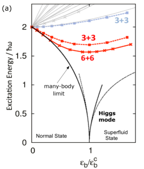
Figure 1: The lowest monopole excitation for $3+3$ fermions (dashed red line) and for $6+6$ fermions (red solid line) obtained by numerical diagonalisation of Eq. (1). The blue dashed line is the second excited state, and the gray solid lines are higher excitations for the $3+3$ system. The black solid (dotted) lines show the numerical (analytic) many-body Higgs-mode energy Bruun (2014) (see Supplementary Material Note (1)).

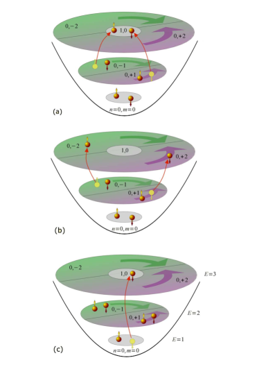
Figure 2: Panels (a) and (b) show a schematic sketch of an excitation of a time-reversed pair $(n,m,\uparrow)$ and $(n,-m,\downarrow)$ one shell up. The energy of such excitations decreases with increasing attraction. Panel (c) shows an example of a single-particle monopole excitation two shells up. The energy of such excitations grows with increasing attraction.

To link the few-body spectrum to the thermodynamic limit, we also plot in Fig. 1 the lowest monopole mode obtained from a many-body calculation, which includes fluctuations around the Bardeen-Cooper-Schrieffer (BCS) solution Bruun (2014) (see Supplementary Material Note (1)). Due to the energy gap in the single particle spectrum for a closed-shell configuration, there is a normal to superfluid quantum phase transition at a critical binding energy $\epsilon_{b}^{c}$. The system is in the normal phase for $\epsilon_{b}<\epsilon_{b}^{c}$, and the lowest monopole mode corresponds to vibrations in the pairing energy $|\Delta|$ around the $\Delta=0$ equilibrium value. The frequency of this mode decreases with increasing attraction and vanishes at $\epsilon_{b}^{c}$, signalling a quantum phase transition to a superfluid phase. In the superfluid phase, the minimum energy is obtained for $|\Delta|>0$, and the Higgs mode corresponds to vibrations in $|\Delta|$ around this minimum. Its energy is approximately given by $2|\Delta|$ (The deviation is due to the breaking of particle-hole symmetry), increasing from zero at the critical point. When $|\Delta|\ll\hbar\omega$, the Cooper pairs are predominantly formed by time-reversed states in the same shell Bruun (2014). Importantly, the Higgs mode is undamped in this regime due to the discrete nature of the trap level spectrum, which is in sharp contrast to the other table top systems mentioned above, where the damping is significant.

Comparing the 3+3 and the many-body spectrum in Fig. 1 clearly shows that the lowest monopole mode for the 3+3 system becomes the few-body precursor of the Higgs mode with increasing attraction. The non-monotonic behaviour of its energy is the smooth few-body analogue of the sharp thermodynamic normal to superfluid quantum phase transition with a vanishing Higgs mode frequency at the critical point. We also show in Fig. 1 the lowest monopole mode for the 6+6 system corresponding to a closed-shell configuration with the three lowest shells filled. The non-monotonic behaviour of the lowest excitation energy is now even more pronounced with a deeper minimum, reflecting the gradual few- to many-body transition with increasing particle number.

In the Supplementary Material Note (1), we illustrate further the few- to many-body transition by calculating the spectrum for the closed shell configurations up to 15+15 particles. Since it is numerically intractable to perform exact diagonalisations of Eq. (1) beyond 6+6 particles, we use a simplified model, which includes only the highest filled and the lowest two empty shells. This calculation clearly shows a pronounced deepening of the minimum of the excitation energy with increasing particle number.

In Fig. 3, we plot the lowest monopole excitations for a $4+4$ system, which corresponds to an open-shell configuration where there is a pair of $\uparrow\downarrow$ particles in the third shell. Contrary to the closed-shell configuration, all excitation energies now increase monotonically with the attraction. This is because there is pairing for any attractive interaction so that the lowest excitations involve pair breaking,

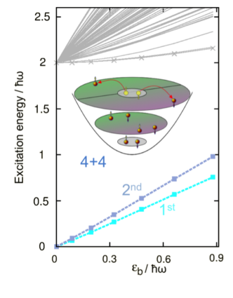
Figure 3: Monopole excitations of an open-shell system. The lowest excitations are intra-shell excitations, which do not exhibit a minimum. The grey lines show higher excitations (which correspond to inter-shell transitions). Inset: Sketch of time-reversed intra-shell pair-excitations.

and it demonstrates that the non-monotonic behaviour of the lowest mode energy is characteristic of a closed-shell configuration, where there is a quantum phase transition in the thermodynamic limit.

In order to investigate further the connection between the few- and many-body physics, we quantify the amount of time-reversed pairing correlations in a given state by

$$P=\sum\limits_{i}\left|C^{tr}_{i}\right|^{2}.$$ (2)

Here, $C_{i}$ are the expansion coefficients in the many-body basis for a given eigenstate. The sum runs over all basis states formed from the non-interacting ground state by excitations of time-reversed (”tr”) pairs. In Fig. 4, we plot $P$ for the ground state and the two lowest excited states.

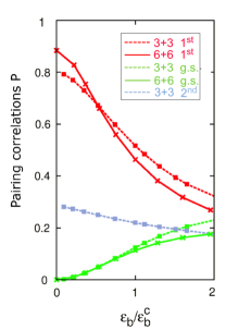
Figure 4: Pairing correlations of the few-body states as defined by Eq. (2) for $N=3+3$ fermions (dashed lines) and $N=6+6$ fermions (solid lines). The green lines show the ground state and the red lines show the first excited state. The blue line shows the second excited state (only for $3+3$).

Comparing the first excited state with the ground state and with the second excited states clearly shows that below the critical binding energy $\epsilon_{b}^{c}$, the wavefunction of the lowest mode is mainly formed by coherent excitations of time-reversed pairs. It is consistent with the canonical many-body picture of vibrations in $|\Delta|$, since such excitations give rise to fluctuations in the pairing field. The higher mode has a significantly smaller proportion of pair correlations, and it mainly consists of single-particle excitations two shells up. The pairing correlations in the ground state increase with increasing attraction, as it becomes more favorable to excite time reversed pairs across the energy gap. This smooth increase of ground state pair correlations is the few-body analogue of the normal to superfluid quantum phase transition, where excitations of time-reversed pairs cost zero energy at the critical coupling strength making the system spontaneously form Cooper pairs. The pair correlated part of the few-body Higgs mode decreases for $\epsilon_{b}>\epsilon_{b}^{c}$, since it is orthogonal to the ground state.

We now address how one can detect the few-body Higgs mode in atomic gas experiments using microtraps. Two experimental probes are widely used: Periodic modulations of the trapping frequency and of the interaction strength. From Fermi’s golden rule, the transition rate from the ground state $|G\rangle$ to an excited state $|E\rangle$ is proportional to the transition matrix elements

$$\Gamma^{E}_{\text{trap}} =|\langle G|\sum_{i}{\mathbf{r}}_{i}^{2}|E\rangle|^{2}$$

$$\Gamma^{E}_{\text{int}} =|\langle G|\sum_{k,l}\delta({\mathbf{r}}_{k}-{\mathbf{r}}_{l})|E\rangle|^{2}$$ (3)

for the two probes. In Fig. 5, we plot $\Gamma^{E}_{\text{trap}}$ and $\Gamma^{E}_{\text{int}}$ to the excited states of the $3+3$ and the $6+6$ systems. Figure 5 (left) shows that the transition rate into the lowest mode is much larger than the rate into the second excited state when the coupling strength is modulated. This is because the interaction operator $\Gamma_{\text{int}}$ can excite time-reversed pairs, (see Supplementary Material Note (1)), which are precisely the excitations that give rise to pair vibrations. Thus, the Higgs mode can be selectively excited by modulating the interaction strength, using for instance a Feshbach resonance. This fact, together with the non-monotonic frequency behaviour, can be used to experimentally identify the Higgs mode. On the other hand, Fig. 5 (right) shows that when the trapping potential is modulated, the transition rate into the second excited state is much larger than into the lowest mode for small attraction. The reason is that $\sum_{i}{\mathbf{r}}_{i}^{2}$ is a single particle operator, whereas the lowest mode mostly consists of time-reversed pair excitations. With increasing attraction, the transition rate into the lowest mode increases, consistent with the fact that the pair correlation $P$ in the Higgs mode decreases with increasing coupling.

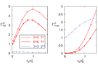
Figure 5: Left: Transition matrix elements $\Gamma^{E}_{\text{int}}$ corresponding to modulating the interaction strength for a $3+3$ and a $6+6$ system. The matrix elements are normalised by $\Gamma^{E}_{\text{int}}$ calculated to the Higgs mode at a very low coupling strength for the $3+3$ system. Right: Transition matrix elements $\Gamma^{E}_{\text{trap}}$ corresponding to modulating the trapping frequency. The matrix elements are normalised by $\Gamma^{E}_{\text{trap}}$ to the second excited state calculated at a very low coupling strength.

In conclusion, we demonstrated using exact diagonalisation that the lowest monopole excitation energy of a two-component Fermi gas exhibits a non-monotonic behaviour with increasing attractive interaction for closed shell configurations. The mode frequency has a minimum in a cross-over region, which deepens as the many-body limit is approached with increasing particle number. Comparing with a many-body calculation, we identified the few-body precursor of the Higgs mode, which has a vanishing frequency at the quantum phase transition point between a normal and a superfluid phase. We showed that the mode is mainly formed by coherent excitations of time-reversed pairs, and that it can be selectively excited by modulating the interaction strength. These results demonstrate how a new generation of cold atom experiments using microtraps can be used to explore two fundamental questions in physics: The nature of the Higgs mode and the cross-over from few- to many-body physics. Our results are also relevant to the nuclear structure community, since we show how cold atoms can be used to probe pair correlations in a finite systems much more systematically compared to what is possible in nuclei Frauendorf and Macchiavelli (2014); Potel et al. (2013).

We end by noting that similar results hold for atoms in a 3D trap Bruun and Mottelson (2001); Bruun (2002). Focus was here on the 2D case, as it is closer to being experimentally realised. Indeed, the first experiment observing pairing correlations in 2D has already been reported Ries et al. (2015).

I Acknowledgements

We thank Ben Mottelson and Sven Åberg for many useful discussions, as well as Jeremy Armstrong for a comparison to a more phenomenological pairing model. We thank Massimo Rontani for discussions regarding the regularization scheme, and also acknowledge discussions with Selim Jochim and Frank Deuretzbacher. This research was financially supported by the Swedish Research Council and NanoLund at Lund University. GMB would like to acknowledge the support of the Villum Foundation via grant VKR023163 and ESF POLATOM network.

II Supplemental Material for ”Few-body precursor of the Higgs mode in a Fermi gas ”

II.1 Many-body theory

To calculate the collective mode spectrum in the many-body limit, we use a BCS mean-field approach combined with Gaussian fluctuation theory. When the trap level spacing is larger than the pairing energy, the Cooper pairs are predominantly formed by intrashell correlations between time-reversed states in the same shell, i.e. $(n,m,\uparrow)$ and $(n,-m,\downarrow)$ Bruun and Heiselberg (2002); Heiselberg and Mottelson (2002). Using this and neglecting the weak angular momentum dependence of the pairing, the mean-field Bogoliubov-de Gennes equations can be reduced to the gap equation Bruun (2014)

$$\sum_{n}\frac{1}{2\sqrt{\xi_{n}^{2}+\Delta_{n}^{2}}}=\sum_{n}\frac{1}{2\epsilon_{n}-E_{2}}.$$ (4)

Here, $\Delta_{n}=\Delta/\sqrt{n+1}$ is the gap for shell $n$, $\epsilon_{n}=(n+1)\hbar\omega$, and $\xi_{n}=\epsilon_{n}-\epsilon_{F}$. The Fermi energy $\epsilon_{F}=(n_{F}+3/2)\hbar\omega$ is between the highest occupied $n_{F}$ and the lowest unoccupied shell $n_{F}+1$. Since there is a gap in the single particle spectrum for a closed shell configuration, there is superfluid pairing only above a critical binding energy $\epsilon_{b}^{c}$.

For small pairing energy, we can expand (4) in $\Delta_{n}/\hbar\omega$ and $\epsilon_{b}/\hbar\omega$. This yields

$$\frac{\epsilon^{c}_{b}}{\omega}=\frac{B(n_{F})}{2\xi(2)}[\sqrt{1+4\xi(2)/B(n_{F})^{2}}-1]$$ (5)

for the critical attraction strength for pairing with $B(n_{F})=\gamma+4\ln 2+\ln n_{F}$. Here $\xi(z)$ is Riemann’s zeta function and $\gamma=0.577$ is the Euler-Mascheroni constant. For $\epsilon_{b}>\epsilon_{b}^{c}$, this expansion yields the approximate solution to the gap equation

$$\Delta_{n_{F}}=\frac{\hbar\omega}{\sqrt{7\xi(3)}}\sqrt{\frac{\hbar\omega}{\epsilon^{c}_{b}}-\frac{\hbar\omega}{\epsilon_{b}}+\xi(2)\left(\frac{\epsilon_{b}}{\hbar\omega}-\frac{\epsilon^{c}_{b}}{\hbar\omega}\right)}.$$ (6)

To describe the collective modes, we include Gaussian fluctuations of the pairing field around the mean-field BCS solution. These can for low energy be split in to phase fluctuations corresponding to Goldstone modes, and amplitude fluctuations corresponding to the Higgs mode. The equation determining the Higgs mode energy $\hbar\omega_{H}$ reads

$$\sum_{n}\frac{2\xi_{n}^{2}}{E_{n}(4\xi_{n}^{2}+4\Delta_{n}^{2}-\hbar^{2}\omega_{H}^{2})}=\sum_{n}\frac{1}{2\epsilon_{n}-E_{2}}.$$ (7)

Assuming perfect particle-hole symmetry around the Fermi level, we see from the gap equation (4) that $\omega=2\Delta_{n_{F}}$ is a solution. In the normal phase for $\epsilon_{b}<\epsilon_{b}^{c}$, (7) has to be solved with $E_{n}=|\xi_{n}|$ and the amplitude modes correspond to coherently either adding or removing a pair of particles. The particle-conserving collective modes correspond to subsequently adding and removing a pair of particles, and their frequencies are therefore twice the frequency obtained by solving (7). Close to the critical coupling strength $\epsilon_{b}\lesssim\epsilon_{b}^{c}$, we expand (7) in $\epsilon_{b}/\hbar\omega$ and $\epsilon/\hbar\omega$ arriving at

$$\frac{\omega_{H}}{\omega}=\frac{2}{\sqrt{7\xi(3)}}\sqrt{\frac{\hbar\omega}{\epsilon_{b}}-\frac{\hbar\omega}{\epsilon^{c}_{b}}+\xi(2)\left(\frac{\epsilon^{c}_{b}}{\hbar\omega}-\frac{\epsilon_{b}}{\hbar\omega}\right)}.$$ (8)

The solid lines in Fig. 1 in the main text are obtained from a numerical solution of (7) for $n_{F}=20$, and the dashed lines are obtained from $2\Delta_{n_{F}}$ using (6) for $\epsilon_{b}>\epsilon_{b}^{c}$, and from (8) for $\epsilon_{b}<\epsilon_{b}^{c}$.

II.2 Interaction and excitation of time-reversed pairs

The interaction term in the Hamiltonian reads in second quantisation

$$H_{\text{int}}\simeq g\sum_{\begin{subarray}{c}nm\\ n^{\prime}m^{\prime}\end{subarray}}\langle nm,n-m|\delta(\mathbf{r}_{1}-\mathbf{r}_{2})|n^{\prime}m^{\prime},n^{\prime}-m^{\prime}\rangle$$

$$\times a_{nm\uparrow}^{\dagger}a_{n-m\downarrow}^{\dagger}a_{n^{\prime}-m^{\prime}\downarrow}a_{n^{\prime}m^{\prime}\uparrow},$$ (9)

where $a_{n_{1}m_{1}\sigma}$ removes a particle with harmonic quantum numbers $(n_{1},m_{1})$ and spin $\sigma$. We have assumed that there are only pair correlations between time reversed states.

Neglecting the weak angular momentum dependence of the matrix element, we can write the interaction in the form

$$H_{\rm int}=G\sum_{nn^{\prime}}\Gamma_{n}^{\dagger}\Gamma_{n^{\prime}}$$ (10)

where $\Gamma_{n}^{\dagger}=\sum_{m}a_{nm\uparrow}^{\dagger}a_{n-m\downarrow}^{\dagger}/\sqrt{n+1}$. The effective coupling strength is

$$G=\frac{2\pi\int_{0}^{\infty}rdr\rho_{n_{F}}^{2}(r)}{n_{F}+1}$$ (11)

where $\rho_{n}(r)$ is the radial density from a full $n$-shell. We see that this interaction precisely excites time-reversed pairs across the energy gap. Modulating the coupling strength $G$ will therefore strongly couple to the Higgs mode.

II.3 Few- to many-body transition in a coreless 2D Harmonic Oscillator

We shall in this section explore the few- to many-body transition further, by calculating the collective mode spectrum for larger particle numbers. Unfortunately, the complexity of the many-body problem makes an exact solution via the configuration interaction (CI) diagonalization method described in the main article numerically intractable for more than 6+6 particles. We therefore turn to an approximate model that nevertheless contains the relevant physics. In the main article, we establish that the formation of the Higgs mode is associated with time-reversed pair excitations from the uppermost filled shell into higher empty shells. The energy of the lowest monopole mode initially decreases with increasing attraction, since the pairs can use the degeneracy of the empty shells to increase their spatial overlap. This effect becomes more pronounced for larger systems with a larger degeneracy of the empty shells. One example of this is the lower minimum in the Higgs excitation energy for the 6+6 system relative to the 3+3 system.

To describe this effect in a simplified numerically tractable system, we consider here a three-level model, where the dynamics of the filled low-lying core of closed shells is ignored assuming that it remains completely filled, see the sketch in Fig. 6. The model includes the three most important single-particle harmonic oscillator shells for the low lying collective modes: the highest filled and the two lowest empty shells for a given closed shell configuration. For example, we approximate the 6+6 system by a three-shell system loaded with 3+3 particles. This simplification allows us to go to much larger particle numbers than what is possible within the full CI scheme.

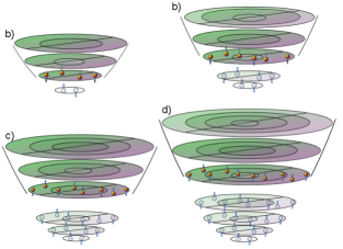
Figure 6: Sketch of the three-level model, where the transparent shells and particles represent the core part of the system, which plays no role in the dynamics. The system with 3+3 particles is approximated by a 2+2 three-shell system (a), 6+6 particles by a three-shell 3+3 system (b), 10+10 particles by a three-shell 4+4 system (c), and 15+15 particles by a three-shell 5+5 system (d).

In Fig. 7, we plot the lowest monopole excitation energy as a function of the coupling strength $|g|m/\hbar^{2}$ of the three-level model for the closed shell configurations up to 15+15 particles. We see that the minimum of the mode energy deepens with increasing particle number, reflecting that the number of degenerate pair excitations increases, which allows for a larger spatial overlap between particles in the upper shells. This clearly demonstrates how with increasing particle number, the finite size system gradually approaches the many-body limit, where the Higgs mode energy vanishes at the critical coupling strength and it costs zero energy to coherently excite pairs across the shells. Note that the excitation energy minimum for the 3+3 system is deeper for the three-level model as compared to that of the full model shown in Fig. 1 in the main article. This is because coherent excitations of time-reversed pairs play a larger role in the three-level model, which has a much smaller phase space as compared to the full model.

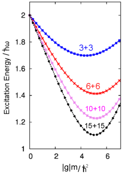
Figure 7: The lowest monopole excitations of the three-shell model for 3+3 (blue line), 6+6 (red line), 10+10 (magenta line) and 15+15 (black line) particles. The results are obtained by exact diagonalization of the full interacting many-body Hamiltonian of the three-shell systems.

III Numerical Calculations

We use two parameters which together define the many-body basis used in our calculations: the single particle energy cut-off $E^{\text{shell}}_{\text{max}}$, and the many-body cut-off $E_{\text{cut}}$. These two cutoff parameters are optimized for each calculation individually in order to reach the best possible convergence. For the transition matrix elements, the comparison between the two different system sizes is more delicate, and we therefore follow a slightly different strategy: The same $E^{\text{shell}}_{\text{max}}$ is used for the $3+3$ and $6+6$ systems, and $E_{\text{cut}}$ is defined so that the maximum many-body excitation energy relative the non-interacting ground state is the same for both systems. In this way, we have a systematic way of comparing matrix elements for the two different system sizes.

III.1 Critical binding energy

In the main manuscript, we divide the two-body binding energy $\epsilon_{b}$ by the critical binding energy $\epsilon_{b}^{c}$ when the excitation energies are plotted, so that we can compare results obtained for different system sizes. The lowest monopole mode will then by definition have the minimum energy at $\epsilon_{b}/\epsilon_{b}^{c}=1$ for all system sizes. Of course, the actual value of $\epsilon_{b}^{c}$ depends on the system size. The exact calculations give $\epsilon_{b}^{c}=0.86\hbar\omega$ for the 3+3 system and $\epsilon_{b}^{c}=0.78\hbar\omega$ for the 6+6 system. This is significantly larger than what is predicted by the many-body expression Eq. (5) for $n_{F}=2$ and $n_{F}=3$. This is not surprising as the systems are small and far from the thermodynamic limit, and since the microscopic model includes all excitations, whereas the many-body theory focuses on the pair excitations.

References

- de Heer (1993) W. A. de Heer, Rev. Mod. Phys. 65, 611 (1993).
- Brack (1993) M. Brack, Rev. Mod. Phys. 65, 677 (1993).
- Reimann and Manninen (2002) S. M. Reimann and M. Manninen, Rev. Mod. Phys. 74, 1283 (2002).
- Serwane et al. (2011) F. Serwane, G. Zürn, T. Lompe, T. B. Ottenstein, A. N. Wenz, and S. Jochim, Science 332, 336 (2011).
- Zürn et al. (2013) G. Zürn, A. N. Wenz, S. Murmann, A. Bergschneider, T. Lompe, and S. Jochim, Phys. Rev. Lett. 111, 175302 (2013).
- Zürn et al. (2012) G. Zürn, F. Serwane, T. Lompe, A. N. Wenz, M. G. Ries, J. E. Bohn, and S. Jochim, Phys. Rev. Lett. 108, 075303 (2012).
- Rontani (2012) M. Rontani, Phys. Rev. Lett. 108, 115302 (2012).
- Wenz et al. (2013) A. N. Wenz, G. Zürn, S. Murmann, I. Brouzos, T. Lompe, and S. Jochim, Science 342, 457 (2013).
- Sowinski (2015) T. Sowinski, Few-Body Syst. 56, 659 (2015).
- Sowinski et al. (2015) T. Sowinski, M. Gajda, and K. Rzazewski, Europhys. Lett. 109, 26005 (2015).
- Grining et al. (2015a) T. Grining, M. Tomza, M. Lesiuk, M. Przybytek, M. Musiał, R. Moszynski, M. Lewenstein, and P. Massignan, Phys. Rev. A 92, 061601 (2015a).
- Grining et al. (2015b) T. Grining, M. Tomza, M. Lesiuk, M. Przybytek, M. Musiał, P. Massignan, M. Lewenstein, and R. Moszynski, New Journal of Physics 17, 115001 (2015b).
- D’Amico and Rontani (2015) P. D’Amico and M. Rontani, Phys. Rev. A 91, 043610 (2015).
- Sachdev (2011) S. Sachdev, Quantum Phase Transitions (Cambridge University Press; 2 edition, 2011).
- Goldstone (1961) J. Goldstone, Il Nuovo Cimento (1955-1965) 19, 154 (1961).
- Higgs (1964) P. W. Higgs, Phys. Rev. Lett. 13, 508 (1964).
- Ryder (1996) L. H. Ryder, Quantum Field Theory, 2nd ed. (Cambridge University Press, 1996).
- CMS collaboration (2012) CMS collaboration, Physics Letters B 716, 30 (2012).
- ATLAS collaboration (2012) ATLAS collaboration, Physics Letters B 716, 1 (2012).
- Bohr and Mottelson (1998) A. Bohr and B. R. Mottelson, Nuclear Structure (World Scientific Publishing Company, 1998).
- Pekker and Varma (2015) D. Pekker and C. Varma, Annual Review of Condensed Matter Physics 6, 269 (2015).
- Cea and Benfatto (2014) T. Cea and L. Benfatto, Phys. Rev. B 90, 224515 (2014).
- Cea et al. (2015) T. Cea, C. Castellani, G. Seibold, and L. Benfatto, Phys. Rev. Lett. 115, 157002 (2015).
- Sherman et al. (2015) D. Sherman, U. S. Pracht, B. Gorshunov, S. Poran, J. Jesudasan, M. Chand, P. Raychaudhuri, M. Swanson, N. Trivedi, A. Auerbach, M. Scheffler, A. Frydman, and M. Dressel, Nat Phys 11, 188 (2015).
- Sooryakumar and Klein (1980) R. Sooryakumar and M. V. Klein, Phys. Rev. Lett. 45, 660 (1980).
- Méasson et al. (2014) M.-A. Méasson, Y. Gallais, M. Cazayous, B. Clair, P. Rodière, L. Cario, and A. Sacuto, Phys. Rev. B 89, 060503 (2014), arXiv:1401.1025 [cond-mat.supr-con] .
- Littlewood and Varma (1981) P. B. Littlewood and C. M. Varma, Phys. Rev. Lett. 47, 811 (1981).
- Rüegg et al. (2008) C. Rüegg, B. Normand, M. Matsumoto, A. Furrer, D. F. McMorrow, K. W. Krämer, H. U. Güdel, S. N. Gvasaliya, H. Mutka, and M. Boehm, Phys. Rev. Lett. 100, 205701 (2008).
- Endres et al. (2012) M. Endres, T. Fukuhara, D. Pekker, M. Cheneau, P. Schauß, C. Gross, E. Demler, S. Kuhr, and I. Bloch, Nature 487, 454 (2012).
- Liu et al. (2015) L. Liu, K. Chen, Y. Deng, M. Endres, L. Pollet, and N. Prokof’ev, Phys. Rev. B 92, 174521 (2015).
- Rontani et al. (2008) M. Rontani, S. Åberg, and S. M. Reimann, ArXiv e-prints (2008), arXiv:0810.4305 .
- Rontani et al. (2009) M. Rontani, J. R. Armstrong, Y. Yu, S. Åberg, and S. M. Reimann, Phys. Rev. Lett. 102, 060401 (2009).
- Note (1) See Supplemental Material [url], which includes Refs. Bruun and Heiselberg (2002); Heiselberg and Mottelson (2002) for details the theory and for more results.
- Bruun and Heiselberg (2002) G. M. Bruun and H. Heiselberg, Phys. Rev. A 65, 053407 (2002).
- Heiselberg and Mottelson (2002) H. Heiselberg and B. Mottelson, Phys. Rev. Lett. 88, 190401 (2002).
- Lehoucq et al. (1998) R. B. Lehoucq, D. C. Sorensen, and C. Yang, ARPACK user’s guide - Solution of large-scale eigenvalue problems with implicitly restarted Arnoldi methods (SIAM, Philadelphia, 1998).
- Randeria et al. (1990) M. Randeria, J.-M. Duan, and L.-Y. Shieh, Phys. Rev. B 41, 327 (1990).
- Zöllner et al. (2011) S. Zöllner, G. M. Bruun, and C. J. Pethick, Phys. Rev. A 83, 021603 (2011).
- Galitskii (1958) V. Galitskii, Soviet Physics JETP 7, 104 (1958).
- Gor’kov and K (1961) L. P. Gor’kov and M.-B. T. K, Sov. Phys.-JETP 13, 1018 (1961).
- Leggett (1980) A. J. Leggett, “Modern trends in the theory of condensed matter: Proceedings of the xvi karpacz winter school of theoretical physics, february 19 – march 3, 1979 karpacz, poland,” (Springer Berlin Heidelberg, Berlin, Heidelberg, 1980) Chap. Diatomic molecules and cooper pairs, pp. 13–27.
- Bruun et al. (1999) G. Bruun, Y. Castin, R. Dum, and K. Burnett, European Physical Journal D 7, 433 (1999), cond-mat/9810013 .
- Stetcu et al. (2007) I. Stetcu, B. R. Barrett, U. van Kolck, and J. P. Vary, Phys. Rev. A 76, 063613 (2007).
- Alhassid et al. (2008) Y. Alhassid, G. F. Bertsch, and L. Fang, Phys. Rev. Lett. 100, 230401 (2008).
- Zinner et al. (2009) N. T. Zinner, K. Mølmer, C. Özen, D. J. Dean, and K. Langanke, Phys. Rev. A 80, 013613 (2009).
- Bruun (2014) G. M. Bruun, Phys. Rev. A 90, 023621 (2014).
- Frauendorf and Macchiavelli (2014) S. Frauendorf and A. O. Macchiavelli, Progress in Particle and Nuclear Physics 78, 24 (2014).
- Potel et al. (2013) G. Potel, A. Idini, F. Barranco, E. Vigezzi, and R. A. Broglia, Reports on Progress in Physics 76, 106301 (2013).
- Bruun and Mottelson (2001) G. M. Bruun and B. R. Mottelson, Phys. Rev. Lett. 87, 270403 (2001).
- Bruun (2002) G. M. Bruun, Phys. Rev. Lett. 89, 263002 (2002).
- Ries et al. (2015) M. G. Ries, A. N. Wenz, G. Zürn, L. Bayha, I. Boettcher, D. Kedar, P. A. Murthy, M. Neidig, T. Lompe, and S. Jochim, Phys. Rev. Lett. 114, 230401 (2015).