Photoproduction of $a_{2}(1320)$ in a Regge model

Abstract

In this work, the photoproduction of $a_{2}(1320)$ off a proton target is investigated within an effective Lagrangian approach and the Regge model. The theoretical result indicates that the shapes of the total and differential cross sections of the $\gamma p\rightarrow a_{2}^{+}n$ reaction within the Feynman (isobar) model are much different from that of the Reggeized treatment. The obtained cross section is compared with the existing experimental results at low energies. The $a_{2}(1320)$ production cross section at high energies can be tested by the COMPASS experiment, which can provide important information for clarifying the role of the Reggeized treatment at that energy range.

I Introduction

Within the past decades great progress has been achieved in hadron spectroscopy mn10 ; liu14 . Especially, inspired by the observation of exotic states mn10 ; liu14 (such as the candidate for the tetraquark ra14 or pentaquark ra15 state etc.), the underlying structure of these states attracts much attention both in theory and experiment. Observation of the exclusive photoproduction of exotic hadronic states off baryons, proposed in the Refs. liu8 ; he09 ; lin14 ; liu15 ; karliner16 , is the most direct way to get information about their nature. At higher energies such processes can be described in terms of Regge trajectory exchanges pd77 ; vg09 . In Ref. wt03 , the $\eta$ and $\eta^{\prime}$ photoproduction were studied with the Reggeized model. It is found that the Reggeized model gives a good description for these reactions in and beyond the resonance region. Thus the photoproduction reaction at high energy may be appropriate to study the role of Reggeized treatment.

In the 1950s, Regge proved the importance of extending the angular momentum $J$ to the complex field regge59 ; regge60 . For more general reviews about the Regge theory, see Refs. rj71 ; tc06 ; jk87 . Later, the exchange of dominant meson Regge trajectories was used to successfully describe the hadron photoproduction mg97 ; gg11 ; he14 ; ew14 . However, there is one question: has the Regge trajectory approach been well tested by experiment at higher energies?

In the past, the $a_{2}(1320)$ ($\equiv a_{2}$) photoproduction was extensively studied. The estimation of the exclusive photoproduction cross section for $a_{2}$ has been performed according to the one-pion exchange (OPE) mechanism with absorption in Hog66 . The experimental results for the values and energy dependence of this cross section at relatively low ($<$20 GeV) energies are quite consistent with the prediction of this model gt93 . Nevertheless the energy range covered by the existing experimental data is not enough to distinguish between the OPE prediction and the Regge trajectory approach mo66 .

The COMPASS experiment at CERN, uses the muon beam, can significantly enlarge the available energy range of virtual photons up to about 150 GeV. COMPASS has a good opportunity to contribute to the study of exotic charmonia via their photoproduction. However the uncertainties of the theoretical description of photon-nucleon interaction at high energies complicate this task. The process of $\gamma^{\ast}p\rightarrow a_{2}^{+}n$, where $\gamma^{\ast}$ is a virtual photon, has quite good experimental signature and can be used as a benchmark. Possibility to use $a_{2}$ photoproduction as a benchmark for study of exotic hadrons is discussed also in cz1 . It is also significant to carry out more theoretical studies on the $\gamma p\rightarrow a_{2}^{+}n$ process in order to clarify the role of the Reggeized treatment.

Moreover, due to the vector meson dominance (VMD) assumption, a photon can interact with a vector meson, which means that the $\gamma p\rightarrow a_{2}^{+}n$ reaction can also proceed through the vector meson dominance (VMD) mechanism tb65 ; tb69 ; th78 . Thus the $a_{2}$ photoproduction mechanism is also an interesting issue.

In this work, the $\gamma p\rightarrow a_{2}^{+}n$ reaction is investigated using an effective Lagrangian approach and the Regge model. In addition to the $\pi$ exchange, the contributions from the VMD mechanism is also considered. The differential cross section of the $\gamma p\rightarrow a_{2}^{+}n$ reaction is also calculated, which could be tested by further COMPASS experiment.

This paper is organized as follows. After the introduction, we present the formalism and the main ingredients which are used in our calculation. The numerical results and discussions are given in Sec. III. In Sec. IV, we give a detailed illustration of the possibility of the experimental test at COMPASS. Finally, the paper ends with a brief summary.

II Formalism

In the present work, an effective Lagrangian approach in terms of hadrons is adopted, which is an important theoretical method in investigating various scattering processes zou03 ; xyw15 ; xy ; epl15 ; epja15 ; xy2940 .

Figure 1 describes the basic tree-level Feynman diagrams for the $a_{2}(1320)$ photoproduction process through general $\pi$ exchange [Fig. 1(a)] and vector meson dominance (VMD) mechanism [Fig. 1(b)] tb65 ; tb69 ; th78 .

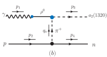
Figure 1: (a): Feynman diagrams for the $\gamma p\rightarrow a_{2}n$ reaction via $\pi$ exchange. (b) same as in (a), but for the case in the frame of the VMD model.

To gauge the contribution of this diagram, we need to know the relevant effective Lagrangian densities.

For the $\pi NN$ interaction vertex we take the effective pseudoscalar coupling kt98 ,

$$\mathcal{L}_{\pi NN}=-ig_{\pi NN}\bar{N}\gamma_{5}\vec{\tau}\cdot\vec{\pi}N$$ (1)

where $\vec{\tau}$ is the Pauli matrix, while $N$ and $\pi$ stand for the fields of the nucleon and the pion, respectively. The coupling constant of the $\pi NN$ interaction was given in many theoretical works, and we take $g_{\pi NN}^{2}/4\pi=12.96$ lzw ; vb11 .

The commonly employed Lagrangian densities for $a_{2}\pi\gamma$ and $a_{2}\pi\rho$ couplings are nl76 ; jb76 ; kb80 ; ze84 :

$$\mathcal{L}_{a_{2}\pi\gamma} = \frac{g_{a_{2}\pi\gamma}}{m_{\pi}^{2}}\epsilon_{\mu\nu\alpha\beta}\partial^{\mu}a_{2}^{\nu\sigma}\partial^{\alpha}A^{\beta}\partial_{\sigma}\phi_{\pi},$$ (2)

$$\mathcal{L}_{a_{2}\pi\rho} = \frac{g_{a_{2}\pi\rho}}{m_{\pi}^{2}}\epsilon_{\mu\nu\alpha\beta}\partial^{\mu}a_{2}^{\nu\sigma}\partial^{\alpha}\rho^{\beta}\partial_{\sigma}\phi_{\pi},$$ (3)

where $A^{\beta}$, $a_{2}^{\nu\sigma}$, $\rho^{\beta}$ and $\phi_{\pi}$ are the photon, $a_{2}$ meson, $\rho$ and $\pi$ fields. $m_{\pi}$ is the mass of the $\pi$ meson. The coupling constant $g_{a_{2}\pi\gamma}$ and $g_{a_{2}\pi\rho}$ can be determined by the partial decay widths $\Gamma_{a_{2}\rightarrow\pi\gamma}$ and $\Gamma_{a_{2}\rightarrow\pi\rho}$, respectively. With the above Lagrangian densities, we obtain

$$\Gamma_{a_{2}\rightarrow\pi\gamma} = \frac{g_{a_{2}\pi\gamma}^{2}}{10\pi m_{\pi}^{4}}\left|\vec{p}_{\gamma}^{~{}\mathrm{c.m.}}\right|^{5},$$ (4)

$$\Gamma_{a_{2}\rightarrow\pi\rho} = \frac{g_{a_{2}\pi\rho}^{2}}{10\pi m_{\pi}^{4}}\left|\vec{p}_{\rho}^{~{}\mathrm{c.m.}}\right|^{5},$$ (5)

with

$$|\vec{p}_{\gamma}^{~{}\mathrm{c.m.}}| = \frac{\lambda^{1/2}(M_{a_{2}}^{2},m_{\pi}^{2},m_{\gamma}^{2})}{2M_{a_{2}}},$$ (6)

$$|\vec{p}_{\rho}^{~{}\mathrm{c.m.}}| = \frac{\lambda^{1/2}(M_{a_{2}}^{2},m_{\pi}^{2},m_{\rho}^{2})}{2M_{a_{2}}},$$ (7)

where $\lambda$ is the K$\ddot{a}$llen function with $\lambda(x,y,z)=(x-y-z)^{2}-4yz$. Using the partial decay widths of $a_{2}(1320)$ as listed in the PDG book pdg , we get $g_{{}_{a_{2}\pi\gamma}}=0.539\times 10^{-2}$ GeV^-1 and $g_{{}_{a_{2}\pi\rho}}=0.268$ GeV^-1.

For the $a_{2}\gamma\pi$ interaction vertex we can also derive it using the vector meson dominance (VMD) mechanism tb65 ; tb69 ; th78 on the assumption that the coupling is due to a sum of intermediate vector mesons. In the VMD mechanism for photoproduction, a real photon can fluctuate into a virtual vector meson, which subsequently scatters from the target proton. Under the VMD mechanism, the Lagrangian of depicting the coupling of the intermediate vector meson $\rho$ with a photon is written as

$$\mathcal{L}_{\rho\gamma}=-\frac{em_{\rho}^{2}}{f_{\rho}}V_{\mu}A^{\mu},$$ (8)

where $m_{\rho}^{2}$ and $f_{\rho}$ are the mass and the decay constant of the $\rho$ meson, respectively. With the above equation, we get the expression for the $\rho\rightarrow e^{+}e^{-}$ decay,

$$\Gamma_{\rho\rightarrow e^{+}e^{-}}=\left(\frac{e}{f_{\rho}}\right)^{2}\frac{8\alpha\left|\vec{p}_{e}^{~{}\mathrm{c.m.}}\right|^{3}}{3m_{\rho}^{2}},$$ (9)

where $\vec{p}_{e}^{~{}\mathrm{c.m.}}$ indicates the three-momentum of an electron in the rest frame of the $\rho$ meson, while $\alpha=e^{2}/4\hbar c=1/137$ is the electromagnetic fine structure constant. Thus, with the partial decay width of $\rho\rightarrow e^{+}e^{-}$ pdg

$$\Gamma_{\rho\rightarrow e^{+}e^{-}}=7.04\text{ keV,}$$ (10)

we get the constant $e/f_{\rho}\simeq 0.06$.

To account for the internal structure of hadrons, we introduce phenomenological form factors. For the vertex of $a_{2}\pi\rho$, the following form factor is adopted xy ; mosel98 ; mosel99 ,

$$\mathcal{F}_{a_{2}\pi\rho}(q_{\pi}^{2})=\frac{m_{\rho}^{2}-m_{\pi}^{2}}{m_{\rho}^{2}-q_{\pi}^{2}}.$$ (11)

For the vertices of $\pi NN$ and $a_{2}\pi\gamma$, three types of the form factors are considered xy ; mosel98 ; mosel99 ; vp16 ; fc16 : (i) the monopole form factor

$$\mathcal{F}_{\pi NN}(q_{\pi}^{2})=\mathcal{F}_{a_{2}\pi\gamma}(q_{\pi}^{2})=\frac{\Lambda_{t}^{2}-m_{\pi}^{2}}{\Lambda_{t}^{2}-q_{\pi}^{2}},$$ (12)

(ii) the dipole form factor

$$\mathcal{F}_{\pi NN}(q_{\pi}^{2})=\mathcal{F}_{a_{2}\pi\gamma}(q_{\pi}^{2})=\left(\frac{\Lambda_{d}^{2}-m_{\pi}^{2}}{\Lambda_{d}^{2}-q_{\pi}^{2}}\right)^{2},$$ (13)

(iii) the exponential form factor

$$\mathcal{F}_{\pi NN}(q_{\pi}^{2})=\mathcal{F}_{a_{2}\pi\gamma}(q_{\pi}^{2})=\exp\left[R^{2}\frac{\left(t-m_{\pi}^{2}\right)}{\left(1-X_{L}\right)}\right],$$ (14)

where $\Lambda_{t},\Lambda_{d}$ and $R$ are the free parameters, which can be determined from the data in this work. $X_{L}$ is momentum fraction of the proton carried by the neutron.

With the effective Lagrangian densities as listed above, the invariant scattering amplitudes for the $\gamma(p_{1})p(p_{2})\rightarrow a_{2}^{+}(p_{3})n(p_{4})$ process can be written as

$$\mathcal{M}_{a} = \sqrt{2}\frac{g_{\pi NN}g_{a_{2}\pi\gamma}}{m_{\pi}^{2}}\frac{\mathcal{F}_{\pi NN}(q_{\pi}^{2})\mathcal{F}_{a_{2}\pi\gamma}(q_{\pi}^{2})}{q_{\pi}^{2}-m_{\pi}^{2}}\bar{u}(p_{4})$$ (15)

$$\times\gamma_{5}\epsilon_{\mu\nu\alpha\beta}p_{3}^{\mu}T^{\nu\sigma}(p3)p_{1}^{\alpha}\epsilon^{\beta}(p_{1})(q_{\pi})_{\sigma}u(p_{2})$$

for Fig. 1(a), and

$$\mathcal{M}_{b} = \sqrt{2}\frac{g_{\pi NN}g_{a_{2}\pi\rho}}{m_{\pi}^{2}}\frac{e}{f_{\rho}}\frac{\mathcal{F}_{\pi NN}(q_{\pi}^{2})\mathcal{F}_{a_{2}\pi\rho}(q_{\pi}^{2})}{q_{\pi}^{2}-m_{\pi}^{2}}\bar{u}(p_{4})$$ (16)

$$\times\gamma_{5}\epsilon_{\mu\nu\alpha\beta}p_{3}^{\mu}T^{\nu\sigma}(p3)p_{1}^{\alpha}\epsilon^{\beta}(p_{1})(q_{\pi})_{\sigma}u(p_{2})$$

for Fig. 1(b). Here $\epsilon^{\beta}(p_{1})$ and $T^{\nu\sigma}(p3)$ are the photon polarization vector and the polarization vector of the $a_{2}$, respectively , $u(p_{2})$ and $\bar{u}(p_{4})$ are the Dirac spinors for the initial proton and final the neutron, respectively.

To describe the behavior at high photon energy, we introduce the Regge trajectories mg97 ; xy ; ai05 ; tc07

$$\frac{1}{q_{\pi}^{2}-m_{\pi}^{2}}\rightarrow\mathcal{D}_{\pi}=(\frac{s}{s_{\text{scale}}})^{\alpha_{\pi}(t)}\frac{\pi\alpha_{\pi}^{\prime}e^{-i\pi\alpha_{\pi}(t)}}{\Gamma[1+\alpha_{\pi}(t)]\sin[\pi\alpha_{K}(t)]},$$ (17)

where $\alpha_{K}^{\prime}$ is the slope of the trajectory and the scale factor $s_{\text{scale}}$ is fixed at 1 GeV², while $s=(p_{1}+p_{2})^{2}$ and $t=(p_{2}-p_{4})^{2}$ are the Mandelstam variables. In addition, the kaonic Regge trajectory $\alpha_{K}(t)$ is mg97 ; xy ; ai05 ; tc07

$$\alpha_{\pi}(t)=0.7(t-m_{\pi}^{2}).$$ (18)

With $s=(p_{1}+p_{2})^{2}$, the unpolarized differential cross section for the $\gamma(p_{1})p(p_{2})\rightarrow a_{2}^{+}(p_{3})n(p_{4})$ process at the center of mass (c.m.) frame is given by

$$\frac{d\sigma}{d\cos\theta}=\frac{1}{32\pi s}\frac{\left|\vec{p}_{3}^{{~{}\mathrm{c.m.}}}\right|}{\left|\vec{p}_{1}^{{~{}\mathrm{c.m.}}}\right|}\left(\frac{1}{4}\sum\limits_{spins}\left|\mathcal{M}_{a/b}\right|^{2}\right)$$ (19)

where $\theta$ denotes the angle of the outgoing $a_{2}^{+}$ meson relative to the beam direction in the c.m. frame, while $\vec{p}_{1}^{{~{}\mathrm{c.m.}}}$ and $\vec{p}_{3}^{{~{}\mathrm{c.m.}}}$ are the three-momenta of the initial photon beam and the final $a_{2}^{+}$, respectively.

III Results and discussion

III.1 Cross section for the $\gamma p\rightarrow a_{2}^{+}n$ reaction

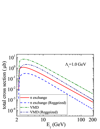
Figure 2: (Color online) Total cross section for the $\gamma p\rightarrow a_{2}^{+}n$ reaction for the fixed parameter $\Lambda_{t}=1$ GeV.

Energy dependence of the cross section calculated above for each of the models for the fixed parameter $\Lambda_{t}=1$ GeV of the monopole form factor is shown in Fig 2. One can see that the difference between the models is about an order of magnitude. Fine tuning of the parameter $\Lambda_{t}$ can be performed on the basis of the experimental results.

The existing experimental data ws75 ; ye72 ; mn09 ; ei69 ; gt93 for $a_{2}$ photoproduction at low energies are summarized in Table I and Fig. 3. The original data from ei69 have been reanalysed in gt93 to take into account the actual branching ratio for $a_{2}\rightarrow 3\pi$ decay channel, since it was taken to be 100%. To fix the same problem we scale the result for the cross section and the error presented in ye72 by the factor of 1.5. We also skip the result for $E_{\gamma}=19.5$ GeV, which seems are in tension with the shape of the expected theoretical curves. The MINUIT code of the CERNLIB library was used to perform one-parameter $\chi^{2}$ fits of the theoretical curves to the $\sigma_{\gamma p\rightarrow a_{2}^{+}n}$ data. The free parameters involved and their fitted values are listed in Table II.

Table 1: The experimental data for $a_{2}$ photoproduction cross section. Here the beam energy $E_{\gamma}$ is in the units of GeV, while the cross section $\sigma_{\gamma p\rightarrow a_{2}^{+}n}$ is the units of $\mu$b.

$E_{\gamma}$	$\sigma_{\gamma p\rightarrow a_{2}^{+}n}$	Data source
3.625 (3.25-4.0)	$0.7\pm 0.3$	ws75
4.2 (3.7-4.7)	$1.2\pm 0.45$	ye72
4.8 (4.3-5.25)	$2.6\pm 0.6$	gt93 ; ei69
5.1 (4.8-5.4)	$0.81\pm 0.25$	mn09
5.15 (4.0-6.3)	$0.3\pm 0.3$	ws75
5.25 (4.7-5.8)	$0.9\pm 0.45$	ye72
7.5 (6.8-8.2)	$0.45\pm 0.45$	ye72
19.5	$0.29\pm 0.06$	gt93

Table 2: The fitted values of the free parameter $\Lambda_{t}$ of the monopole form factor, while the cutoff $\Lambda_{t}$ is in the units of GeV.

type	$\Lambda_{t}$	$\chi^{2}/ndf$
$\pi$ exchange	0.99$\pm 0.07$	2.23
$\pi$ exchange(Reggeized)	3.58$\pm 0.66$	2.73
VMD	0.35$\pm 0.02$	2.05
VMD(Reggeized)	0.46$\pm 0.04$	2.04

Table 3: The fitted values of the free parameter $\Lambda_{d}$ of the dipole form factor, while the cutoff $\Lambda_{d}$ is in the units of GeV.

type	$\Lambda_{d}$	$\chi^{2}/ndf$
$\pi$ exchange	1.53$\pm 0.11$	2.26
$\pi$ exchange(Reggeized)	3.79$\pm 0.78$	2.91
VMD	0.54$\pm 0.03$	2.07
VMD(Reggeized)	0.69$\pm 0.06$	2.05

Table 4: The fitted values of the free parameter $R$ of the exponential form factor, while $R$ is in the units of GeV^-1.

type	$R$	$\chi^{2}/ndf$
$\pi$ exchange	0.47$\pm 0.03$	2.26
$\pi$ exchange(Reggeized)	0.10$\pm 0.02$	2.66
VMD	1.30$\pm 0.07$	2.10
VMD(Reggeized)	1.06$\pm 0.09$	2.06

The fitted parameter $\Lambda_{t}$ satisfys the expectation with a reasonable $\chi^{2}/{ndf}$. And yet, it is found that the cases with Reggeized treatment need a larger $\Lambda_{t}$. For comparison, we also calculate the result with dipole or exponential form factor. The fitted parameter $\Lambda_{d}$ and $R$ are listed in Table III and Table IV, respectively. Fig. 3 show that the fitted results with the three types of form factor. It is found that the difference is small the result of improvements in three types of form factor. Therefore, in the following calculation, we only consider the case of monopole form factor.

From Fig. 3(a) one can see that the experimental data (except the point at $E_{\gamma}=4.8and19.5$ GeV)ws75 ; ye72 ; mn09 ; gt93 ; ei69 for the total cross section of the $\gamma p\rightarrow a_{2}^{+}n$ reaction are well reproduced with a small value of $\chi^{2}{/ndf}$. The shape of the total cross section via $\pi$ exchange is different from that of the VMD mechanism.

With the above equations and the fitted parameters as listed in Table II, the relevant physical results are calculated, as shown in Fig. 4-6.

In Fig. 4 we also present the variation of the total cross section of the $\gamma p\rightarrow a_{2}^{+}n$ reaction within the typical uncertainties of the $\Lambda_{t}$ values. From Fig. 4 (a) it is seen that the total cross section via $\pi$ exchange is more sensitive than that of the VMD mechanism to the values of $\Lambda_{t}$. Moreover, a comparison of the results from Fig. 4 (a) and Fig. 4 (b) reveals that the total cross section becomes less sensitive to the $\Lambda_{t}$ values when the Reggeized treatment is added to the process of $\gamma p\rightarrow a_{2}^{+}n$.

In Fig. 5, we show the differential cross section of $\gamma p\rightarrow a_{2}^{+}n$ as a function of $-t$. It is obvious that there is a significant peak structure in the region of low $-t$, which increases rapidly near the threshold and then decreases slowly with increasing $-t$. However, it is seen, that the shapes of the differential cross section $d\sigma/dt$ with the Reggeized treatment are much different from that without the Reggeized treatment at higher $-t$. The Reggeized treatment can lead to that the differential cross section $d\sigma/dt$ decreases rapidly with increasing $-t$, especially at higher energies.

Figure 6 presents the differential cross section for the $\gamma p\rightarrow a_{2}^{+}n$ reaction with or without the Reggeized treatment at different energies. It is seen that the differential cross section with the Reggeized treatment is very sensitive to the angle $\theta$ and makes a considerable contribution at forward angles.

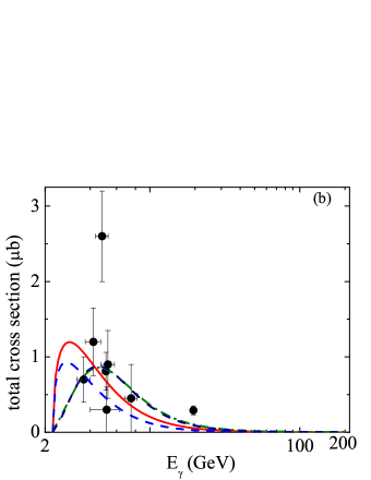
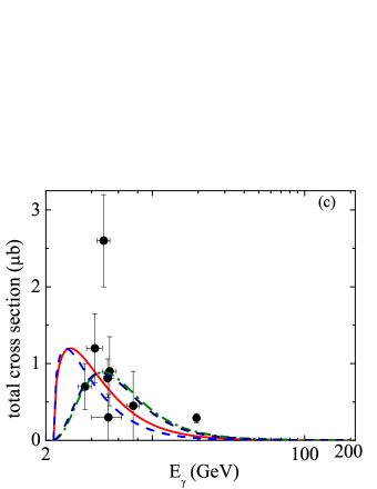
Figure 3: (Color online) Total cross section for the $\gamma p\rightarrow a_{2}^{+}n$ reaction. The datas are from ws75 ; ye72 ; mn09 ; gt93 ; ei69 . Here, (a) is the result with monopole form factor, while (b) and (c) are the results related to the dipole and exponential form factors correspondently.

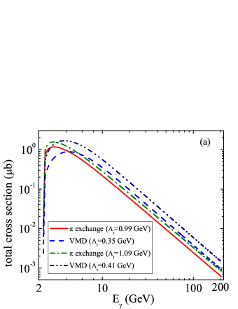
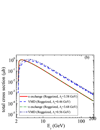
Figure 4: (Color online) (a): The total cross section of the $\gamma p\rightarrow a_{2}^{+}n$ reaction for the different values of cutoff parameter $\Lambda_{t}$. (b) same as in (a), but for the case of the Regge trajectory exchange.

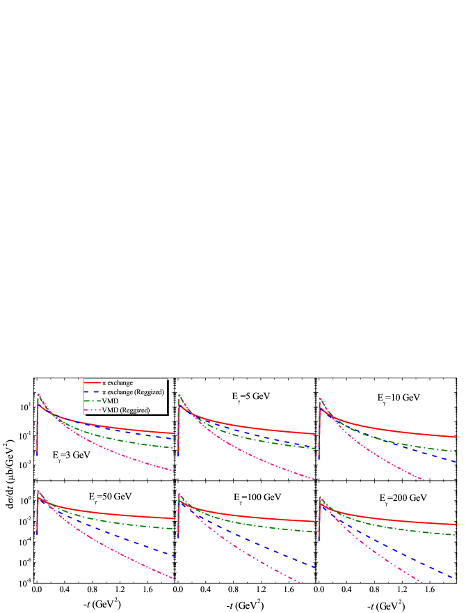
Figure 5: (Color online) The differential cross section of $\gamma p\rightarrow a_{2}^{+}n$ as a function of $-t$ at $E_{\gamma}=3-200$ GeV.

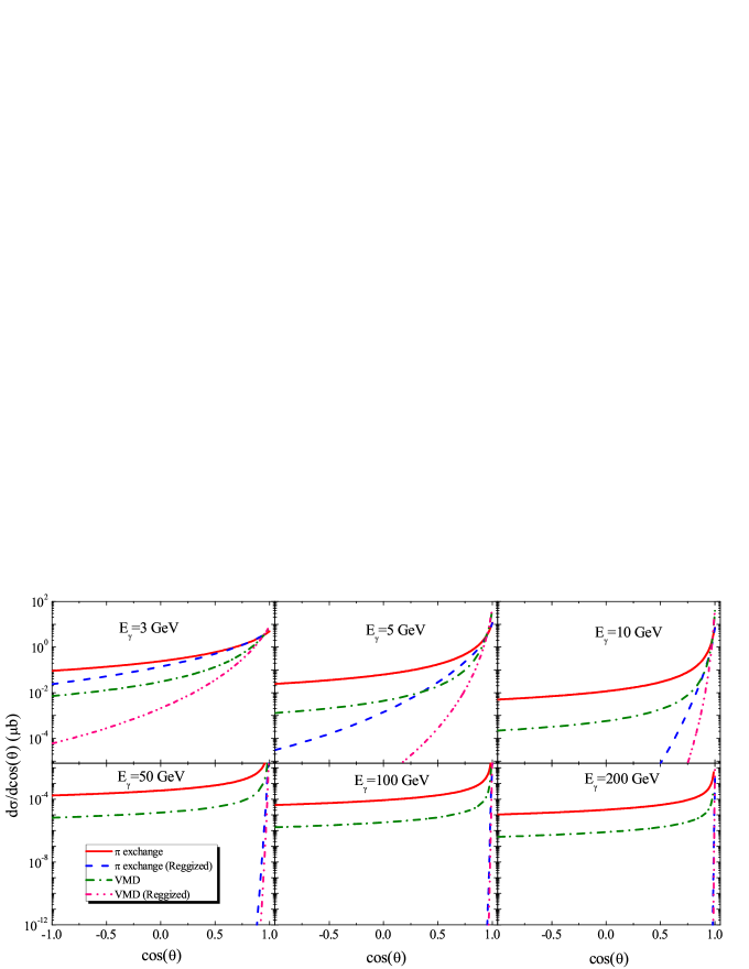
Figure 6: (Color online) The differential cross section $d\sigma/d\cos\theta$ for the $a_{2}(1320)$ photoproduction from the protron as a function of $\cos\theta$ at $E_{\gamma}=3-200$ GeV.

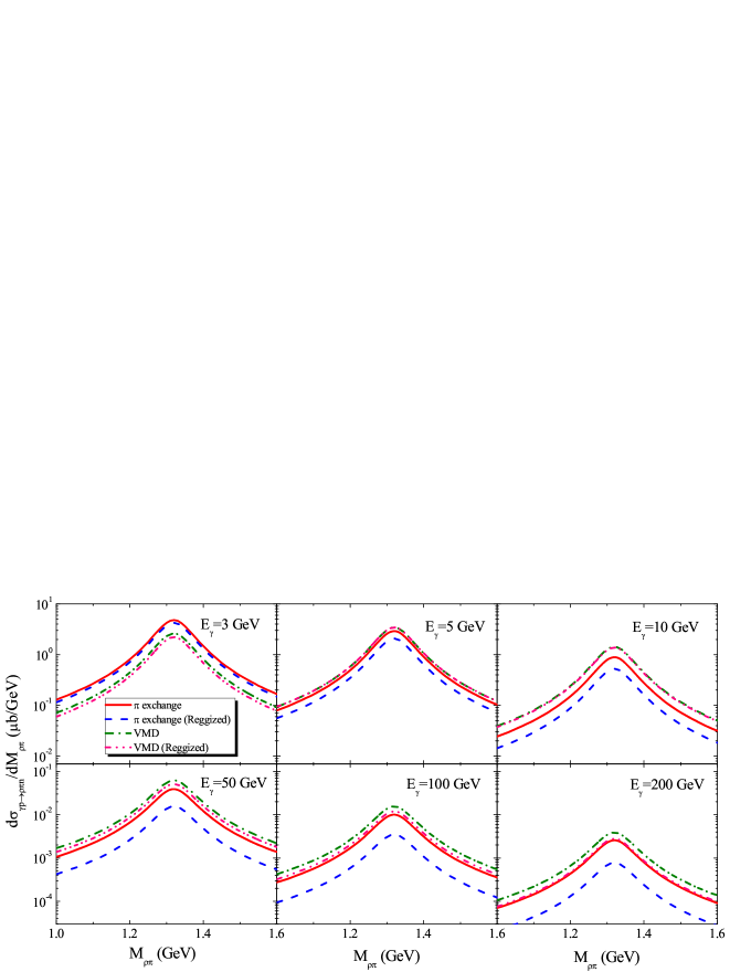
Figure 7: (Color online) Differential cross section $d\sigma_{\gamma p\rightarrow a_{2}^{+}n\rightarrow\rho\pi n}/dM_{\rho\pi}$ as a function of $M_{\rho\pi}$ at $E_{\gamma}=3-200$ GeV.

III.2 Dalitz process $\gamma p\rightarrow\rho\pi n$

Considering the $a_{2}$ are usually detected in experiment via the $\rho\pi$ invariant mass , it would be useful to give the theoretical predictions of the differential cross section $d\sigma_{\gamma p\rightarrow a_{2}^{+}n\rightarrow\rho\pi n}/dM_{\rho\pi}$ as a function of the beam energy $E_{\gamma}$, which could be tested by further experiment. Since the full decay width of the $a_{2}(1320)$ is small enough in comparison to its mass, the invariant mass distribution for the Dalitz process $\gamma p\rightarrow\rho\pi n$ can be defined with the two-body process sn15

$$\frac{d\sigma_{\gamma p\rightarrow\rho\pi n}}{dM_{\rho\pi}}\approx\frac{2m_{a_{2}}M_{\rho\pi}}{\pi}\frac{\sigma_{\gamma p\rightarrow a_{2}^{+}n}\Gamma_{a_{2}\rightarrow\rho\pi}}{(M_{\rho\pi}^{2}-m_{a_{2}}^{2})^{2}+m_{a_{2}}^{2}\Gamma_{a_{2}}^{2}},$$

where the full width $\Gamma_{a_{2}}=107$ MeV and the partial width $\Gamma_{a_{2}\rightarrow\rho\pi}=75$ MeV are taken pdg .

With the above equations and the fitted parameters as listed in Table II, the invariant-mass distribution $d\sigma_{\gamma p\rightarrow a_{2}^{+}n\rightarrow\rho\pi n}/dM_{\rho\pi}$ for $E_{\gamma}=3-200$ GeV is calculated, as shown in Fig. 7. It is seen that there exists an obvious peak at $M_{\rho\pi}\approx 1.32$ GeV.

IV Possibility of the experimental test at COMPASS 

The COMPASS experiment Abbon:2007pq is situated at the M2 beam line of the CERN Super Proton Synchrotron. Since 2002 it has obtained experimental data for positive muons scattering of 160 $GeV/c$ (2002-2010) or 200 $GeV/c$ momentum (2011) off solid ⁶LiD (2002-2004) or NH₃ polarized targets (2006-2011). Particle tracking and identification is performed in a two-stage spectrometer covering a wide kinematical range. The trigger system comprises hodoscope counters and hadron calorimeters.

According to the presented calculations of the $a_{2}$ production cross section and previously published COMPASS results for exclusive photoproduction of $\rho^{0}$ rho0 and $J/\psi$ Jpsi we can conclude that thousands of $a_{2}^{\pm}$ mesons could be produced per year of data taking via the exclusive charge-exchange reactions $\gamma^{\ast}p\rightarrow a_{2}^{+}n$ and $\gamma^{\ast}n\rightarrow a_{2}^{-}p$ (but the recoil nucleon cannot be detected). The energy of a virtual photon covers the range from about 20 GeV and up to 180 GeV. The obtained data can be used to clarify the mechanism of the $a_{2}$ production and the role of the Reggeized treatment at high energies. Nevertheless, most of the $a_{2}^{\pm}$ mesons at such energies are produced non exclusively via the pomeron exchange mechanism. Such events could produce strong background under poor exclusivity control. Additional systematics could come from the process $\gamma^{\ast}p\rightarrow a_{2}^{-}\Delta^{++}$ (the cross section of this reaction is of the same order of magnitude DeltaPP ) because the COMPASS setup is not able to reconstruct a decay of low-energy $\Delta^{++}$ in a regular way. Nuclear effects in $a_{2}$ photoproduction off the lithium-6, deuterium and nitrogen nuclei should also be taken into account in an appropriate way.

The forthcoming upgrade of the COMPASS setup related to the planned data taking within the framework of the GPD program COMPASS_proposal could provide better conditions for experimental study of the reaction $\gamma^{\ast}p\rightarrow a_{2}^{+}n$ and partially eliminate problems mentioned above. The new 2.5 m long liquid hydrogen target surrounded by a 4 m long recoil proton detector will be used. Absence of the neutrons in the target will remove one exclusive production channel for $a_{2}^{-}$. The recoil proton detector serves the double purpose: to reconstruct and identify recoil protons via time-of-flight and energy loss measurements. Since the reaction $\gamma^{\ast}p\rightarrow a_{2}^{+}n$ does not have a recoil proton in the final state, any activity in the recoil proton detector could be used as the veto in the offline analysis. In addition, the recoil proton detector will be able to detect the $\Delta^{++}\rightarrow p\pi^{+}$ decay. Significant impact on the exclusivity control efficiency will be made by the planned upgrade of the electromagnetic calorimetry system.

V Summary

Within the framework of the effective Lagrangian approach and Regge model, the $a_{2}(1320)$ photoproduction from the proton is investigated.

The obtained numerical results indicate the following:

• The total cross section $\gamma p\rightarrow a_{2}^{+}n$ related to the experimental data ws75 ; ye72 ; mn09 ; ei69 ; gt93 is well reproduced with reasonable value of $\chi^{2}{/ndf}$. Although the monopole form factor was used in the calculations, the dipole and exponential form factors were also tested. It is found that the total cross section becomes less sensitive to the $\Lambda_{t}$ values when the Reggeized treatment is added.

• The shapes of the differential cross section $d\sigma/dt$ with the Reggeized treatment are much different from that without the Reggeized treatment at higher $-t$. The Reggeized treatment can lead to that the differential cross section $d\sigma/dt$ decreases rapidly with the increasing $-t$, especially at higher energies.

• The differential cross section $d\sigma/d\cos\theta$ with the Reggeized treatment is very sensitive to the angle $\theta$ and makes a considerable contribution at forward angles.

• The invariant mass distribution for the Dalitz process $\gamma p\rightarrow\rho\pi n$ shows an obvious peak at $M_{\rho\pi}\approx 1.32$ GeV, which can be checked by further experiment.

• For comparison, it is found that the cross section of the $\gamma n\rightarrow a_{2}^{-}p$ process is almost the same as that of the $\gamma p\rightarrow a_{2}^{+}n$ reaction. Thus, the above theoretical results are valid to the $\gamma n\rightarrow a_{2}^{-}p$ channel.

To sum up, we suggest testing our prediction for the cross section of the $\gamma p\rightarrow a_{2}^{+}n$ process at the COMPASS facility at CERN. Such a test could provide important information for clarifying the production mechanism of the $a_{2}(1320)$ and the role of the Reggeized treatment at high energies. Nevertheless, the precise measurements near the threshold, where the difference between the predictions of the production models is maximal, are also important.

VI Acknowledgments

The author X. Y. Wang is grateful Helmut Haberzettl and Jun He for useful discussions about Regge theory.

References

- (1) M. Nielsen, F. S. Navarra and S. H. Lee, Phys. Rept. 497, 41 (2010).
- (2) X. Liu, Chin. Sci. Bull. 59, 3815 (2014).
- (3) R. Aaij et al. (LHCb Collaboration), Phys. Rev. Lett. 112, 222002 (2014).
- (4) R. Aaij et al. (LHCb Collaboration), Phys. Rev. Lett. 115, 072001 (2015).
- (5) X. Liu et al. Phys. Rev. D 77 094005 (2008).
- (6) J. He, X. Liu, Phys. Rev. D 80 114007 (2009).
- (7) Q. Lin et al. Phys. Rev. D 89 034016 (2014).
- (8) Q. Wang et al. Phys. Rev. D 92 034022 (2015).
- (9) M. Karliner, J. Rosner, Phys. Lett. B 752 329 (2016).
- (10) D. Morrison, Phys. Lett. 22, 528 (1966).
- (11) P. D. B. Collins, “An Introduction to Regge Theory and High Energy Physics High Energy Physics” (Cambridge University Press, 1977).
- (12) V. Gribov, “Strong Interactions of Hadrons at High Energies” (Cambridge University Press, 2009).
- (13) W. T. Chiang et al., Phys. Rev. C 68, 045202 (2003).
- (14) T. Regge, Nuovo Cimento 14, 951 (1959).
- (15) T. Regge, Nuovo Cimento 18, 947 (1960).
- (16) R. J. Eden, Rep. Prog. Phys. 34, 995 (1971).
- (17) T. Corthals, J. Ryckebusch, and T. Van Cauteren, Phys. Rev. C 73, 045207 (2006).
- (18) J. K. Storrow, Rep. Prog. Phys. 50, 1229 (1987).
- (19) M. Guidal, J. M. Laget, and M. Vanderhaeghen, Nucl. Phys. A 627, 645 (1997).
- (20) G. Galat, Phys. Rev. C 83, 065203 (2011).
- (21) J. He, Phys. Rev. C 89, 055204 (2014).
- (22) E. Wang et al., Phys. Rev. C 90, 065203 (2014).
- (23) H. Högaasen et al. Nuovo Cimento 42A, 323 (1966)
- (24) A. P. Szczepaniak and M. Swat, Phys. Lett. B516 72-76 (2001).
- (25) T. Bauer and D. R. Yennie, Phys. Lett. 60B, 165 (1976).
- (26) T. Bauer and D. R. Yennie, Phys. Lett. 60B, 169 (1976).
- (27) T. H. Bauer, et al., Rev. Mod. Phys. 50, 261 (1978); 51, 407(E) (1979).
- (28) B. S. Zou, F. Hussain, Phys. Rev. C 67, 015204 (2003).
- (29) X. Y. Wang, J. J. Xie and X. R. Chen, Phys. Rev. D 91, 014032 (2015).
- (30) X. Y. Wang, X. R. Chen and Alexey Guskov, Phys. Rev. D 92, 094017 (2015).
- (31) X. Y. Wang and X. R. Chen, Europhys. Lett. 109, 41001 (2015).
- (32) X. Y. Wang and X. R. Chen, Eur. Phys. J. A 51 85 (2015).
- (33) X. Y. Wang, Alexey Guskov and X. R. Chen, Phys. Rev. D 92, 094032 (2015).
- (34) K. Tsushima, et al., Phys. Rev. C 59, 369 (1999), Erratum-ibid. Phys. Rev. C 61, 029903 (2000).
- (35) Z. Lin, C. M.Ko, and B. Zhang, Phys. Rev. C 61, 024904 (2000).
- (36) V. Baru, C. Hanhart, M. Hoferichter, B. Kubis, A. Nogga, and D. R. Phillips, Nucl. Phys. A 872, 69 (2011).
- (37) N. Levy, P. Singer and S. Toaff, Phys. Rev. D 13, 2662 (1976).
- (38) J. Babcock and J. L. Rosner, Phys. Rev. D 14, 1286 (1976).
- (39) K. Bongardt, W. Gampp and H. Genz, Z. Phys. C 3, 233 (1980).
- (40) Z. E. S. Uy, Phys. Rev. D 29, 574 (1984).
- (41) K. A. Olive et al. (Particle Data Group), Chin. Phys. C 38, 090001 (2014).
- (42) T. Feuster and U. Mosel, Phys. Rev. C 58, 457 (1998).
- (43) T. Feuster and U. Mosel, Phys. Rev. C 59, 460 (1999).
- (44) V. P. Goncalves, F. S. Navarra and D. Spiering, arXiv:1510.01512 [hep-ph].
- (45) F. Carvalho, V. P. Goncalves, D. Spiering and F. S. Navarra, Phys. Lett. B 752, 76 (2016).
- (46) A. I. Titov et al., Phys. Rev. C 72, 035206 (2005); 72, 049901(E) (2005).
- (47) T. Corthals et al., Phys. Rev. C 75, 045204 (2007).
- (48) W. Struczinski et al. (Aachen-Hamburg-Heidelberg-Munich Collaboration), Nucl.Phys. B 108, 45 (1976).
- (49) Y. Eisenberg et al., Phys. Rev. D 5, 15 (1972).
- (50) M. Nozar et al. (CLAS Collaboration), Phys. Rev. Lett. 102, 102002 (2009).
- (51) Y. Eisenberg et al., Phys. Rev. Lett. 23,1322 (1969)
- (52) G. T. Condo Phys. Rev. D 48, 3045 (1993).
- (53) S. I. Nam and H. K. Jo, arXiv:1503.00419 [hep-ph].
- (54) P. Abbon et al. (COMPASS Collaboration), Nucl. Instrum. Meth. A577, 455 (2007), [arXiv:0703049 [hep-ex]].
- (55) C. Adolph et al., Phys. Lett. B 731, 19 (2014).
- (56) C. Adolph et al. (COMPASS Collaboration), Phys. Lett. B 742, 330 (2015).
- (57) G. T. Condo et al., Phys. Rev. D 41, 3317 (1990).
- (58) COMPASS, SPSC-2010-014/P-340.