Multiscale asymptotics for the Skeleton of the Madden-Julian Oscillation and Tropical–Extratropical Interactions

Shengqian Chen 111Corresponding author Department of Mathematics, University of Wisconsin – Madison, Madison, Wisconsin, USA, sqchen@math.wisc.edu Andrew J. Majda Department of Mathematics, and Center for Atmosphere-Ocean Sciences, Courant Institute of Mathematical Science, New York University, New York, New York, USA, jonjon@cims.nyu.edu Samuel N. Stechmann Department of Mathematics, and Department of Atmospheric and Oceanic Sciences, University of Wisconsin – Madison, Madison, Wisconsin, USA, stechmann@wisc.edu
Abstract

A new model is derived and analyzed for tropical–extratropical interactions involving the Madden–Julian oscillation (MJO). The model combines (i) the tropical dynamics of the MJO and equatorial baroclinic waves and (ii) the dynamics of barotropic Rossby waves with significant extratropical structure, and the combined system has a conserved energy. The method of multiscale asymptotics is applied to systematically derive a system of ordinary differential equations (ODEs) for three-wave resonant interactions. Two novel features are (i) a degenerate auxiliary problem with overdetermined equations due to a compatibility condition (meridional geostrophic balance) and (ii) cubic self-interaction terms that are not typically found in three-wave resonance ODEs. Several examples illustrate applications to MJO initiation and termination, including cases of (i) the MJO, equatorial baroclinic Rossby waves, and barotropic Rossby waves interacting, and (ii) the MJO, baroclinic Kelvin waves, and barotropic Rossby waves interacting. Resonance with the Kelvin wave is not possible here if only dry variables are considered, but it occurs in the moist model here through interactions with water vapor and convective activity.

1 Introduction

The Madden-Julian Oscillation (MJO) is the dominant component of intraseasonal (\approx30-60 days) variability in the tropics [10, 11, 12]. It is an equatorial wave envelope of complex multi-scale convective processes, coupled with planetary-scale (\approx10,000-40,000 km) circulation anomalies. Individual MJO events propagate eastward at a speed of roughly 5 m/s, and their convective signal is most prominent over the Indian and western Pacific Oceans [39]. In addition to its significance to its own right, the MJO also significantly affects many other components of the atmosphere-ocean-earth system, such as monsoon development, intraseasonal predictability in mid-latitude, and the development of the El Nin~~n\tilde{\text{n}}o southern oscillation (ENSO) [8, 39].

In addition to its strong tropical signal, the MJO interacts with the global flow on the intraseaonsal timescales. Teleconnection patterns between the global extratropics and the MJO were described in an early observational analysis by Weickmann (1983) [36] and Weikmann et al. (1985) [38]. Their results demonstrate coherent fluctuations between extratropical flow and eastward-propagating outgoing longwave radiation (OLR) anomalies in the tropics. In the study by Matthews and Kiladis (1999) [21], they illustrate the interplay between high-frequency transient extratropical waves and the MJO. More recently, Weickmann and Berry (2009) [37] demonstrate that convection in the MJO frequently evolves together with a portion of the activity in a global wind oscillation.

The interactions between extratropical waves and tropical convection have also been investigated in numerical models. To view the extratropical response to convective heating, Jin and Hoskins (1995) [4] forced a primitive equation model with a fixed heat source in the tropics in the presence of a climatological background flow and obtain the Rossby wave train response in the result. To diagnose the more specific response to patterns of convection more like those of the observed MJO, Matthews et al. (2004) [20] forced a primitive equation model in a climatological background flow with patterns of observed MJO. The resulting global response to that heating is similar in many respects to the observational analysis. The MJO initiation in response to extratropical waves was illustrated by Ray and Zhang (2010) [27]. They show that a dry-channel model of the tropical atmosphere developed MJO-like signals in tropical wind fields when forced by reanalysis fields at poleward boundaries. Many other interesting studies on tropical–extratropical interactions have been carried out. For example, see Lin et. al. (2009) [9] and Frederiksen and Frederiksen (1993) [3] , and the review by Roundy (2011) [32].

How can one model the two-way interaction between MJO and extratropical waves in a simplified, integrative way? This is the primary question of the present paper. Section 2 introduces a planetary scale model for this purpose. The model includes (i) barotropic dynamics that span the tropics and extratropics, (ii) equatorial baroclinic dynamics, and (iii) the interactive effects of moisture and convection. More specifically, the model integrates the dry barotropic-first baroclinic interaction that has been studied by Majda and Biello (2003) [14] and Khouider and Majda (2005)[5] with the MJO skeleton model first developed by Majda and Stechmann (2009) [18] and further investigated by same authors [19]. The term “skeleton” used by the authors refers to the fundamental features of the MJO on planetary/intraseasonal scales. In these previous studies, Majda and Biello (2003) carry out a multiscale asymptotic analysis for the resonant interactions of dry baroclinic Rossby waves and barotropic Rossby waves; and the MJO skeleton model [18] has captured three main features of the MJO on planetary/intraseasonal scales: (i) slow eastward phase speed of roughly 5m/s; (ii) peculiar dispersion relation with dω/dk0d𝜔d𝑘0\mathrm{d}\omega/\mathrm{d}k\approx 0; (iii) horizontal quadrupole vortex structure.

A multiscale asymptotic analysis is presented here in Section 3 and later sections, adopting similar strategies as in Majda and Biello (2003), based on long-wave scales, small amplitude assumption, and multiple long time scales. The long-wave scaling leads to meridional geostrophic balance at the leading order, which appears as a constraint in the partial differential equation (PDE) system. This constraint complicates the auxiliary problem of the multiscale analysis. In brief, the auxiliary problem is a necessary step for suppressing secular terms. The complication here, which arises from the constraint, is a degenerate operator, which we rectify through a change of basis as described in Section 4. Section 5 presents the dispersion relation of the leading order linear operator for both the baroclinic and barotropic modes. In Section 6, by inspecting the dispersion curves of the linear operator, three-wave resonant interactions are identified, and an ODE system for wave interactions is derived using multiscale asymptotics. A novel feature of this ODE system is the presence of cubic self-interactions terms, which are not typically found in three-wave interaction ODEs (e.g., [1, 13, 23, 30, 31]). Here the cubic self-interaction arises from the new nonlinearity in the MJO skeleton model involving water vapor and convective activity. Many previous studies have been presented on resonant interactions of atmospheric waves, and they usually focused on “dry dynamics” (e.g., [2, 15, 24, 25, 26, 28, 29]). See Khouider et. al. (2013) [6] for a review.

Readers who are most interested in physical applications can skip ahead to Section 6, where the reduced ODE model is presented. The results with the model are then organized as follows. First, in Section 7, a validation study is presented to explore the time scales of validity of the asymptotic model. Second, in Section 8, numerical simulations are presented for three-wave interactions. Two cases of three-wave interactions are chosen for application to MJO initiation and termination [27, 33] and tropical–extratropical interaction. Each case therefore involves both the MJO and barotropic Rossby waves, and the third wave is either a dry baroclinic Rossby wave or a dry Kelvin wave. Interactions involving only the Kelvin wave and the barotropic Rossby waves are not possible, but by including the MJO mode from the model with water vapor and convection, the Kelvin waves are engaged in the resonance triad.

The details of the multiscale asymptotic analysis are presented in the appendices. In Appendix A and B, a meridional truncated system is formulated. Appendix C provides the explicit formulation of the auxiliary problems. Finally, the details of the derivation of the reduced ODE system are given in Appendix D.

2 The two-layer equatorial β𝛽\beta-plane equations

Par. Derivation Dim. val. Description
β𝛽\beta 2.3×10112.3superscript10112.3\times 10^{-11} m-1s-1 Variation of Coriolis parameter with latitude
θ0subscript𝜃0\theta_{0} 300300300 K Potential temperature at surface
g𝑔g 9.89.89.8 m s-2 Gravitational acceleration
H𝐻H 161616 km Tropopause height
N2superscript𝑁2N^{2} (g/θ0)dθ¯/dz𝑔subscript𝜃0d¯𝜃d𝑧(g/\theta_{0})\mathrm{d}\bar{\theta}/\mathrm{d}z 104superscript10410^{-4} s-2 Buoyancy frequency squared
c𝑐c NH/π𝑁𝐻𝜋NH/\pi 505050 m s-1 Velocity scale
Xesubscript𝑋𝑒X_{e} c/β𝑐𝛽\sqrt{c/\beta} 150015001500 km Equatorial length scale
T𝑇T Xe/csubscript𝑋𝑒𝑐X_{e}/c 888 hrs Equatorial time scale
HN2θ0/(πg)𝐻superscript𝑁2subscript𝜃0𝜋𝑔HN^{2}\theta_{0}/(\pi g) 151515 K Potential temperature scale
H/π𝐻𝜋H/\pi 555 km Vertical length scale
H/(πT)𝐻𝜋𝑇H/(\pi T) 0.20.20.2 m s-1 Vertical velocity scale
c2superscript𝑐2c^{2} 250025002500 m2 s-2 Pressure scale
Table 1: Constants and reference scales for nondimensionalization.

The nondimensional two-layer equatorial β𝛽\beta-plane equations for the barotropic and baroclinic MJO skeleton model are given by

𝐯¯t+𝐯¯𝐯¯+y𝐯¯+p¯=12(𝐯𝐯),¯𝐯𝑡¯𝐯¯𝐯𝑦superscript¯𝐯perpendicular-to¯𝑝12tensor-product𝐯𝐯\displaystyle\frac{\partial{\overline{\mathbf{v}}}}{\partial t}+{\overline{\mathbf{v}}}\cdot\nabla{\overline{\mathbf{v}}}+y{\overline{\mathbf{v}}}^{\perp}+\nabla{\overline{p}}=-\frac{1}{2}\nabla\cdot({\mathbf{v}}\otimes{\mathbf{v}}), (1a)
𝐯¯=0,¯𝐯0\displaystyle\nabla\cdot{\overline{\mathbf{v}}}=0, (1b)
𝐯t+𝐯¯𝐯θ+y𝐯=𝐯𝐯¯,𝐯𝑡¯𝐯𝐯𝜃𝑦superscript𝐯perpendicular-to𝐯¯𝐯\displaystyle\frac{\partial{\mathbf{v}}}{\partial t}+{\overline{\mathbf{v}}}\cdot\nabla{\mathbf{v}}-\nabla\theta+y{\mathbf{v}}^{\perp}=-{\mathbf{v}}\cdot\nabla{\overline{\mathbf{v}}}, (1c)
θt+𝐯¯θ𝐯=δ2(H¯aSθ),𝜃𝑡¯𝐯𝜃𝐯superscript𝛿2¯𝐻𝑎superscript𝑆𝜃\displaystyle\frac{\partial\theta}{\partial t}+{\overline{\mathbf{v}}}\cdot\nabla\theta-\nabla\cdot{\mathbf{v}}=\delta^{2}({\bar{H}}a-{S^{\theta}}), (1d)
qt+𝐯¯q+Q~𝐯=δ2(H¯aSq),𝑞𝑡¯𝐯𝑞~𝑄𝐯superscript𝛿2¯𝐻𝑎superscript𝑆𝑞\displaystyle\frac{\partial q}{\partial t}+{\overline{\mathbf{v}}}\cdot\nabla q+\tilde{Q}\nabla\cdot{\mathbf{v}}=-\delta^{2}({\bar{H}}a-{S^{q}}), (1e)
at=Γqa.𝑎𝑡Γ𝑞𝑎\displaystyle\frac{\partial a}{\partial t}=\Gamma qa. (1f)

These equations combine the MJO skeleton model [18] and nonlinear interactions between the baroclinic and barotropic modes [14]. The equations have been nondimensionalized using the scales listed in Table 1. Here 𝐯¯=(u¯,v¯)¯𝐯¯𝑢¯𝑣{\overline{\mathbf{v}}}=({\overline{u}},{\overline{v}}) and p¯¯𝑝{\overline{p}} are barotropic velocity and pressure; 𝐯=(u,v)𝐯𝑢𝑣{\mathbf{v}}=(u,v) and θ𝜃\theta are baroclinic velocity and potential temperature; and q𝑞q is water vapor (sometimes referred to as “moisture”). The tropical convective activity envelope is denoted by δ2asuperscript𝛿2𝑎\delta^{2}a, where δ𝛿\delta is a small parameter that modulates the scales of tropical convection envelope. Likewise, δ2superscript𝛿2\delta^{2} is also applied to quantities Sθsuperscript𝑆𝜃{S^{\theta}} and Sqsuperscript𝑆𝑞{S^{q}}, radiative cooling and the moisture source. In this paper, δ2Sθsuperscript𝛿2superscript𝑆𝜃\delta^{2}{S^{\theta}} and δ2Sqsuperscript𝛿2superscript𝑆𝑞\delta^{2}{S^{q}} are set to be constants for energy conservation, although they usually have both spatial and temporal variance in reality. Together with ΓΓ\Gamma, H¯¯𝐻{\bar{H}} and Q~~𝑄{\tilde{Q}}, the coefficients are described in table 2.

Par. Non-dim. val. Dim. val. Description
ΓΓ\Gamma 1 similar-to\sim0.5 /day/(g/kg) Convective growth/decay rate
H¯¯𝐻{\bar{H}} 0.23 similar-to\sim10 K/day Parameter to rescale a𝑎a
δ2a¯superscript𝛿2¯𝑎\delta^{2}{\bar{a}} δ2superscript𝛿2\delta^{2} Convective activity envelope at RCE state
Q~~𝑄{\tilde{Q}} 0.9 Non-dim. background vertical moisture gradient
δ2Sθsuperscript𝛿2superscript𝑆𝜃\delta^{2}{S^{\theta}} δ2H¯superscript𝛿2¯𝐻\delta^{2}{\bar{H}} Radiative cooling rate
δ2Sqsuperscript𝛿2superscript𝑆𝑞\delta^{2}{S^{q}} δ2H¯superscript𝛿2¯𝐻\delta^{2}{\bar{H}} Moisture source
Table 2: Parameters of the MJO skeleton model, and relation to small parameter δ𝛿\delta.

In equations (1), 𝐯=(v,u)superscript𝐯perpendicular-to𝑣𝑢{\mathbf{v}}^{\perp}=(-v,u) is the β𝛽\beta-plane approximation of tropical Coriolis force, and x𝑥x and y𝑦y denote the zonal and meridional coordinates. Without the moisture q𝑞q and convection envelope a𝑎a, system (1) is the two-vertical-mode Galerkin truncation for the Boussinesq equations with rigid-lid boundary on the top and bottom of the domain (see e.g., [22, 16, 14, 5]) Without the barotropic wind 𝐯¯¯𝐯{\overline{\mathbf{v}}}, the system is the MJO skeleton model on the first baroclinic mode before passing to the long wave limit (see e.g., [18, 19]).

Note that for the primitive equations (1), a total energy is conserved, and it is composed of four parts, dry barotropic energy Tsubscript𝑇\mathcal{E}_{T}, dry baroclinic energy Csubscript𝐶\mathcal{E}_{C}, moisture energy Msubscript𝑀\mathcal{E}_{M}, and convective energy Asubscript𝐴\mathcal{E}_{A}:

T(t)subscript𝑇𝑡\displaystyle\mathcal{E}_{T}(t) =12YY0X|𝐯¯|2dxdyabsent12superscriptsubscript𝑌𝑌superscriptsubscript0𝑋superscript¯𝐯2differential-d𝑥differential-d𝑦\displaystyle=\frac{1}{2}\int_{-Y}^{Y}\int_{0}^{X}|{\overline{\mathbf{v}}}|^{2}\mathrm{d}x\mathrm{d}y (2a)
C(t)subscript𝐶𝑡\displaystyle\mathcal{E}_{C}(t) =14YY0X|𝐯|2+θ2dxdyabsent14superscriptsubscript𝑌𝑌superscriptsubscript0𝑋superscript𝐯2superscript𝜃2d𝑥d𝑦\displaystyle=\frac{1}{4}\int_{-Y}^{Y}\int_{0}^{X}|{\mathbf{v}}|^{2}+\theta^{2}\mathrm{d}x\mathrm{d}y (2b)
M(t)subscript𝑀𝑡\displaystyle\mathcal{E}_{M}(t) =14YY0X1Q~(1Q~)(q+Q~θ)2dxdyabsent14superscriptsubscript𝑌𝑌superscriptsubscript0𝑋1~𝑄1~𝑄superscript𝑞~𝑄𝜃2differential-d𝑥differential-d𝑦\displaystyle=\frac{1}{4}\int_{-Y}^{Y}\int_{0}^{X}\frac{1}{{\tilde{Q}}(1-{\tilde{Q}})}(q+{\tilde{Q}}\theta)^{2}\mathrm{d}x\mathrm{d}y (2c)
A(t)subscript𝐴𝑡\displaystyle\mathcal{E}_{A}(t) =δ22YY0X1Q~Γ[H¯aSθlog(a)]dxdyabsentsuperscript𝛿22superscriptsubscript𝑌𝑌superscriptsubscript0𝑋1~𝑄Γdelimited-[]¯𝐻𝑎superscript𝑆𝜃𝑎differential-d𝑥differential-d𝑦\displaystyle=\frac{\delta^{2}}{2}\int_{-Y}^{Y}\int_{0}^{X}\frac{1}{{\tilde{Q}}\Gamma}\left[{\bar{H}}a-{S^{\theta}}\log(a)\right]\mathrm{d}x\mathrm{d}y (2d)

This energy conservation forms the design principle as appeared in [18, 14]. Note that in (1f), the conserved quantity \mathcal{E} still holds if a𝑎a is also advected by the barotropic wind, i.e., with an additional term u¯a¯𝑢𝑎{\overline{u}}\cdot\nabla a in (1f). But we do not include this term because later, when meridional truncation is applied to the system, the energy conservation will not hold with this additional term.

Using the streamfunction ψ𝜓\psi for barotropic mode, which satisfies (u¯,v¯)=(ψy,ψx)¯𝑢¯𝑣subscript𝜓𝑦subscript𝜓𝑥({\overline{u}},{\overline{v}})=(-\psi_{y},\psi_{x}), the barotropic equation can also be written as

DDtΔψ+ψx+12[(𝐯u)y+(𝐯v)x]=0,𝐷𝐷𝑡Δ𝜓subscript𝜓𝑥12delimited-[]subscript𝐯𝑢𝑦subscript𝐯𝑣𝑥0\frac{D}{Dt}\Delta\psi+\psi_{x}+\frac{1}{2}\nabla\cdot\left[-({\mathbf{v}}u)_{y}+({\mathbf{v}}v)_{x}\right]=0, (3)

where

DDt=t+u¯x+v¯y𝐷𝐷𝑡𝑡¯𝑢𝑥¯𝑣𝑦\frac{D}{Dt}=\frac{\partial}{\partial t}+{\overline{u}}\frac{\partial}{\partial x}+{\overline{v}}\frac{\partial}{\partial y}

represents advection by the barotropic wind.

2.1 The zonal-long wave scaled model

To consider the planetary scale of the coupled equations in (3) and (1c)-(1f), zonal variations are assumed to depend on a longer scale, as are temporal variations. The long zonal and long temporal coordinates are defined as

x=δx,t=δt.formulae-sequencesuperscript𝑥𝛿𝑥superscript𝑡𝛿𝑡x^{\prime}=\delta x,\qquad t^{\prime}=\delta t. (4)

Correspondingly, the meridional velocity is also scaled so that

v=δv.𝑣𝛿superscript𝑣v=\delta v^{\prime}. (5)

The equations in (3) and (1c)-(1f) become the long-wave-scaled system:

DDtψyy+ψx12[(𝐯u)y]+δ2{DDtψxx+12[(𝐯v)x]}=0,𝐷𝐷superscript𝑡subscript𝜓𝑦𝑦subscript𝜓superscript𝑥12superscriptdelimited-[]subscriptsuperscript𝐯𝑢𝑦superscript𝛿2𝐷𝐷superscript𝑡subscript𝜓superscript𝑥superscript𝑥12superscriptdelimited-[]subscriptsuperscript𝐯superscript𝑣superscript𝑥0\displaystyle\frac{D}{Dt^{\prime}}\psi_{yy}+\psi_{x^{\prime}}-\frac{1}{2}\nabla^{\prime}\cdot\left[({\mathbf{v}}^{\prime}u)_{y}\right]+\delta^{2}\left\{\frac{D}{Dt^{\prime}}\psi_{x^{\prime}x^{\prime}}+\frac{1}{2}\nabla^{\prime}\cdot\left[({\mathbf{v}}^{\prime}v^{\prime})_{x^{\prime}}\right]\right\}=0, (6a)
DDtuθxyu𝐯ψy=0,𝐷𝐷superscript𝑡𝑢subscript𝜃𝑥𝑦𝑢superscript𝐯superscriptsubscript𝜓𝑦0\displaystyle\frac{D}{Dt^{\prime}}u-\theta_{x}-yu-{\mathbf{v}}^{\prime}\cdot\nabla^{\prime}\psi_{y}=0, (6b)
θy+yu+δ2(DDtv+vψx)=0subscript𝜃𝑦𝑦𝑢superscript𝛿2𝐷𝐷superscript𝑡superscript𝑣superscript𝑣superscriptsubscript𝜓superscript𝑥0\displaystyle-\theta_{y}+yu+\delta^{2}\left(\frac{D}{Dt^{\prime}}v^{\prime}+v^{\prime}\cdot\nabla^{\prime}\psi_{x^{\prime}}\right)=0 (6c)
DDtθ𝐯δ(H¯aSθ)=0,𝐷𝐷superscript𝑡𝜃superscriptsuperscript𝐯𝛿¯𝐻𝑎superscript𝑆𝜃0\displaystyle\frac{D}{Dt^{\prime}}\theta-\nabla^{\prime}\cdot{\mathbf{v}}^{\prime}-\delta({\bar{H}}a-{S^{\theta}})=0, (6d)
DDtq+Q~𝐯+δ(H¯aSq)=0,𝐷𝐷superscript𝑡𝑞~𝑄superscriptsuperscript𝐯𝛿¯𝐻𝑎superscript𝑆𝑞0\displaystyle\frac{D}{Dt^{\prime}}q+\tilde{Q}\nabla^{\prime}\cdot{\mathbf{v}}^{\prime}+\delta({\bar{H}}a-{S^{q}})=0, (6e)
δtaΓqa=0.𝛿superscript𝑡𝑎Γ𝑞𝑎0\displaystyle\delta\frac{\partial}{\partial t^{\prime}}a-\Gamma qa=0. (6f)

Here the primes represent the long-wave scaled coordinates and variables:

DDt=t+ux+vy,=(x,y),and𝐯¯=(u,v).formulae-sequence𝐷𝐷superscript𝑡superscript𝑡𝑢superscript𝑥superscript𝑣superscript𝑦formulae-sequencesuperscriptsuperscript𝑥𝑦andsuperscript¯𝐯𝑢superscript𝑣\frac{D}{Dt^{\prime}}=\frac{\partial}{\partial t^{\prime}}+u\frac{\partial}{\partial x^{\prime}}+v^{\prime}\frac{\partial}{\partial y^{\prime}},\quad\nabla^{\prime}=(\frac{\partial}{\partial x^{\prime}},\frac{\partial}{\partial y}),\quad\text{and}\quad{\overline{\mathbf{v}}}^{\prime}=(u,v^{\prime}).

System (6) is in the same form as in [14] when the moisture and convection are neglected.

Furthermore, the convective activity a𝑎a will be written as an anomaly from the state of radiative-convective equilibrium (RCE):

Sθ=Sq=H¯a¯,superscript𝑆𝜃superscript𝑆𝑞¯𝐻¯𝑎{S^{\theta}}={S^{q}}={\bar{H}}{\bar{a}},

where these constants take the values given in table 2. When a=a¯𝑎¯𝑎a={\bar{a}}, the external radiative cooling/moisture source is in balance with the source/sink from the convection, and the system achieves RCE. By writing a𝑎a as an anomaly with respect to the RCE value a¯¯𝑎\bar{a}, the forcing terms in (6d) and (6e) can be written as

H¯aSθ=H¯aSq=H¯(aa¯)=H¯a,¯𝐻𝑎superscript𝑆𝜃¯𝐻𝑎superscript𝑆𝑞¯𝐻𝑎¯𝑎¯𝐻superscript𝑎{\bar{H}}a-{S^{\theta}}={\bar{H}}a-{S^{q}}={\bar{H}}(a-{\bar{a}})={\bar{H}}a^{\prime}, (7)

and the equation for the convection envelope (6f) can be written as

taΓa¯q=Γaq.superscript𝑡superscript𝑎Γ¯𝑎𝑞Γsuperscript𝑎𝑞\frac{\partial}{\partial t^{\prime}}a^{\prime}-\Gamma{\bar{a}}q=\Gamma a^{\prime}q. (8)

2.2 Long time scales for tropical–extratropical interactions

The small parameter δ𝛿\delta is also used for introducing two longer time scales:

T1=δt,T2=δ2t.formulae-sequencesubscript𝑇1𝛿superscript𝑡subscript𝑇2superscript𝛿2superscript𝑡T_{1}=\delta t^{\prime},\quad T_{2}=\delta^{2}t^{\prime}.

Their units match the units of intraseasonal timescales as appeared in [14, 17].

In the next section, the system is expanded by matching the orders of δ𝛿\delta.

3 Asymptotic expansions for the interaction of barotropic and equatorial baroclinic waves

In this section, asymptotic expansions are carried out twice: first for the 2-D system as functions of x𝑥x and y𝑦y, and second for a system using a truncated basis for variations in the y𝑦y direction. The first expansion (2-D) provides the clearest presentation, but the 2-D linear operator does not have eigenvalues and eigenfunctions that are easily accessible. For this reason, the second, truncated system is introduced and provides a linear operator with known eigenvalues and eigenfunctions.

3.1 The 2-D equations

Assume that the solutions have an asymptotic structure with ansatz:

(ψ,u,v,θ,q)𝜓𝑢superscript𝑣𝜃𝑞\displaystyle(\psi,u,v^{\prime},\theta,q) =δ2(ψ1,u1,v1,θ1,q1)+δ3(ψ2,u2,v2,θ2,q2)absentsuperscript𝛿2subscript𝜓1subscript𝑢1subscript𝑣1subscript𝜃1subscript𝑞1superscript𝛿3subscript𝜓2subscript𝑢2subscript𝑣2subscript𝜃2subscript𝑞2\displaystyle=\delta^{2}(\psi_{1},u_{1},v_{1},\theta_{1},q_{1})+\delta^{3}(\psi_{2},u_{2},v_{2},\theta_{2},q_{2})
+δ4(ψ3,u3,v3,θ3,q3)+O(δ5)superscript𝛿4subscript𝜓3subscript𝑢3subscript𝑣3subscript𝜃3subscript𝑞3𝑂superscript𝛿5\displaystyle+\delta^{4}(\psi_{3},u_{3},v_{3},\theta_{3},q_{3})+O(\delta^{5}) (9a)
and aand superscript𝑎\displaystyle\text{and }\qquad\qquad a^{\prime} =δa1+δ2a2+δ3a3+O(δ4),absent𝛿subscript𝑎1superscript𝛿2subscript𝑎2superscript𝛿3subscript𝑎3𝑂superscript𝛿4\displaystyle=\delta a_{1}+\delta^{2}a_{2}+\delta^{3}a_{3}+O(\delta^{4}), (9b)

This small amplitude assumption is consistent with a small Froude number assumption as in [14]. All variables are assumed to depend on three time scales: tsuperscript𝑡t^{\prime} and T1=δtsubscript𝑇1𝛿superscript𝑡T_{1}=\delta t^{\prime} and T2=δ2tsubscript𝑇2superscript𝛿2superscript𝑡T_{2}=\delta^{2}t^{\prime}. The system is expanded over three orders of magnitude.

The first order system is

ψ1yyt+ψ1x=0,subscript𝜓1superscript𝑦superscript𝑦superscript𝑡subscript𝜓1superscript𝑥0\displaystyle\psi_{1y^{\prime}y^{\prime}t^{\prime}}+\psi_{1x^{\prime}}=0, (10a)
u1tθ1xyv1=0,subscript𝑢1superscript𝑡subscript𝜃1superscript𝑥superscript𝑦subscript𝑣10\displaystyle u_{1t^{\prime}}-\theta_{1x^{\prime}}-y^{\prime}v_{1}=0, (10b)
θ1y+yu1=0,subscript𝜃1superscript𝑦superscript𝑦subscript𝑢10\displaystyle-\theta_{1y^{\prime}}+y^{\prime}u_{1}=0, (10c)
θ1tu1xv1yH¯a1=0,subscript𝜃1superscript𝑡subscript𝑢1superscript𝑥subscript𝑣1superscript𝑦¯𝐻subscript𝑎10\displaystyle\theta_{1t^{\prime}}-u_{1x^{\prime}}-v_{1y^{\prime}}-{\bar{H}}a_{1}=0, (10d)
q1t+Q~(u1x+v1y)+H¯a1=0,subscript𝑞1superscript𝑡~𝑄subscript𝑢1superscript𝑥subscript𝑣1superscript𝑦¯𝐻subscript𝑎10\displaystyle q_{1t^{\prime}}+\tilde{Q}(u_{1x^{\prime}}+v_{1y^{\prime}})+{\bar{H}}a_{1}=0, (10e)
a1tΓa¯q1=0.subscript𝑎1superscript𝑡Γ¯𝑎subscript𝑞10\displaystyle a_{1t^{\prime}}-\Gamma{\bar{a}}q_{1}=0. (10f)

This system defines the leading-order linear operator, including a combination of barotropic Rossby waves [14] from the dynamics of ψ𝜓\psi and baroclinic equatorial long-waves including the MJO [18] from the other variables.

The second order system is

ψ2yyt+ψ2x=ψ1yyT1,subscript𝜓2superscript𝑦superscript𝑦superscript𝑡subscript𝜓2superscript𝑥subscript𝜓1superscript𝑦superscript𝑦subscript𝑇1\displaystyle\psi_{2y^{\prime}y^{\prime}t^{\prime}}+\psi_{2x^{\prime}}=-\psi_{1y^{\prime}y^{\prime}T_{1}}, (11a)
u2tθ2xyv2=u1T1,subscript𝑢2superscript𝑡subscript𝜃2superscript𝑥superscript𝑦subscript𝑣2subscript𝑢1subscript𝑇1\displaystyle u_{2t^{\prime}}-\theta_{2x^{\prime}}-y^{\prime}v_{2}=-u_{1T_{1}}, (11b)
θ2y+yu2=0,subscript𝜃2superscript𝑦superscript𝑦subscript𝑢20\displaystyle-\theta_{2y^{\prime}}+y^{\prime}u_{2}=0, (11c)
θ2tu2xv2yH¯a2=θ1T1,subscript𝜃2superscript𝑡subscript𝑢2superscript𝑥subscript𝑣2superscript𝑦¯𝐻subscript𝑎2subscript𝜃1subscript𝑇1\displaystyle\theta_{2t^{\prime}}-u_{2x^{\prime}}-v_{2y^{\prime}}-{\bar{H}}a_{2}=-\theta_{1T_{1}}, (11d)
q2t+Q~(u2x+v2y)+H¯a2=q1T1,subscript𝑞2superscript𝑡~𝑄subscript𝑢2superscript𝑥subscript𝑣2superscript𝑦¯𝐻subscript𝑎2subscript𝑞1subscript𝑇1\displaystyle q_{2t^{\prime}}+\tilde{Q}(u_{2x^{\prime}}+v_{2y^{\prime}})+{\bar{H}}a_{2}=-q_{1T_{1}}, (11e)
a2tΓa¯q2=a1T1+Γa1q1.subscript𝑎2superscript𝑡Γ¯𝑎subscript𝑞2subscript𝑎1subscript𝑇1Γsubscript𝑎1subscript𝑞1\displaystyle a_{2t^{\prime}}-\Gamma{\bar{a}}q_{2}=-a_{1T_{1}}+\Gamma a_{1}q_{1}. (11f)

Note that the only nonlinear term is from the q𝑞q-a𝑎a interaction: Γa1q1Γsubscript𝑎1subscript𝑞1\Gamma a_{1}q_{1}.

The third order system is

ψ3yyt+ψ3x=ψ1yyT2ψ2yyT1subscript𝜓3superscript𝑦superscript𝑦superscript𝑡subscript𝜓3superscript𝑥subscript𝜓1superscript𝑦superscript𝑦subscript𝑇2subscript𝜓2superscript𝑦superscript𝑦subscript𝑇1\displaystyle\psi_{3y^{\prime}y^{\prime}t^{\prime}}+\psi_{3x^{\prime}}=-\psi_{1y^{\prime}y^{\prime}T_{2}}-\psi_{2y^{\prime}y^{\prime}T_{1}}
[ψ1xxt+ψ1xψ1yyyψ1yψ1xyy12(u12)xy12(u1v1)yy],delimited-[]subscript𝜓1superscript𝑥superscript𝑥superscript𝑡subscript𝜓1superscript𝑥subscript𝜓1superscript𝑦superscript𝑦superscript𝑦subscript𝜓1superscript𝑦subscript𝜓1superscript𝑥superscript𝑦superscript𝑦12subscriptsuperscriptsubscript𝑢12superscript𝑥superscript𝑦12subscriptsubscript𝑢1subscript𝑣1superscript𝑦superscript𝑦\displaystyle\qquad-\left[\psi_{1x^{\prime}x^{\prime}t^{\prime}}+\psi_{1x^{\prime}}\psi_{1y^{\prime}y^{\prime}y^{\prime}}-\psi_{1y^{\prime}}\psi_{1x^{\prime}y^{\prime}y^{\prime}}-\frac{1}{2}(u_{1}^{2})_{x^{\prime}y^{\prime}}-\frac{1}{2}(u_{1}v_{1})_{y^{\prime}y^{\prime}}\right], (12a)
u3tθ3xyv3=u1T2u2T1[ψ1xu1yψ1yu1xu1ψ1xyv1ψ1yy],subscript𝑢3superscript𝑡subscript𝜃3superscript𝑥superscript𝑦subscript𝑣3subscript𝑢1subscript𝑇2subscript𝑢2subscript𝑇1delimited-[]subscript𝜓1superscript𝑥subscript𝑢1superscript𝑦subscript𝜓1superscript𝑦subscript𝑢1superscript𝑥subscript𝑢1subscript𝜓1superscript𝑥superscript𝑦subscript𝑣1subscript𝜓1superscript𝑦superscript𝑦\displaystyle u_{3t^{\prime}}-\theta_{3x^{\prime}}-y^{\prime}v_{3}=-u_{1T_{2}}-u_{2T_{1}}-\left[\psi_{1x^{\prime}}u_{1y^{\prime}}-\psi_{1y^{\prime}}u_{1x^{\prime}}-u_{1}\psi_{1x^{\prime}y^{\prime}}-v_{1}\psi_{1y^{\prime}y^{\prime}}\right], (12b)
θ3y+yu3=v1t,subscript𝜃3superscript𝑦superscript𝑦subscript𝑢3subscript𝑣1superscript𝑡\displaystyle-\theta_{3y^{\prime}}+y^{\prime}u_{3}=-v_{1t^{\prime}}, (12c)
θ3tu3xv3yH¯a3=θ1T2θ2T1ψ1xθ1y+ψ1yθ1x,subscript𝜃3superscript𝑡subscript𝑢3superscript𝑥subscript𝑣3superscript𝑦¯𝐻subscript𝑎3subscript𝜃1subscript𝑇2subscript𝜃2subscript𝑇1subscript𝜓1superscript𝑥subscript𝜃1superscript𝑦subscript𝜓1superscript𝑦subscript𝜃1superscript𝑥\displaystyle\theta_{3t^{\prime}}-u_{3x^{\prime}}-v_{3y^{\prime}}-{\bar{H}}a_{3}=-\theta_{1T_{2}}-\theta_{2T_{1}}-\psi_{1x^{\prime}}\theta_{1y^{\prime}}+\psi_{1y^{\prime}}\theta_{1x^{\prime}}, (12d)
q3t+Q~(u3x+v3y)+H¯a3=q1T2q2T1ψ1xq1y+ψ1yq1x,subscript𝑞3superscript𝑡~𝑄subscript𝑢3superscript𝑥subscript𝑣3superscript𝑦¯𝐻subscript𝑎3subscript𝑞1subscript𝑇2subscript𝑞2subscript𝑇1subscript𝜓1superscript𝑥subscript𝑞1superscript𝑦subscript𝜓1superscript𝑦subscript𝑞1superscript𝑥\displaystyle q_{3t^{\prime}}+\tilde{Q}(u_{3x^{\prime}}+v_{3y^{\prime}})+{\bar{H}}a_{3}=-q_{1T_{2}}-q_{2T_{1}}-\psi_{1x^{\prime}}q_{1y^{\prime}}+\psi_{1y^{\prime}}q_{1x^{\prime}}, (12e)
a3tΓa¯q3=a1T2a2T1+Γ(a1q2+a2q1)ψ1xa1y+ψ1ya1x.subscript𝑎3superscript𝑡Γ¯𝑎subscript𝑞3subscript𝑎1subscript𝑇2subscript𝑎2subscript𝑇1Γsubscript𝑎1subscript𝑞2subscript𝑎2subscript𝑞1subscript𝜓1superscript𝑥subscript𝑎1superscript𝑦subscript𝜓1superscript𝑦subscript𝑎1superscript𝑥\displaystyle a_{3t^{\prime}}-\Gamma{\bar{a}}q_{3}=-a_{1T_{2}}-a_{2T_{1}}+\Gamma(a_{1}q_{2}+a_{2}q_{1})-\psi_{1x^{\prime}}a_{1y^{\prime}}+\psi_{1y^{\prime}}a_{1x^{\prime}}. (12f)

Note that more nonlinear terms arise, including the baroclinic–barotropic interactions as in [14].

The total energy is approximately conserved:

ddt(3)=o(δ4).ddsuperscript𝑡superscript3𝑜superscript𝛿4\frac{\mathrm{d}}{\mathrm{d}t^{\prime}}\mathcal{E}^{(3)}=o(\delta^{4}). (13)

from the asymptotic expansions (10)-(12), where (3)superscript3\mathcal{E}^{(3)} is the energy of the variables from the leading 3 orders of magnitude from the ansatz in (9). This approximated energy conservation is important to preserve in future derivations.

The asymptotic expansions (10)-(12) are analogous to the expansions in [14], where the system did not have moisture q𝑞q nor convection envelope a𝑎a. Nonetheless, there are essential differences described in table 3. For example, in [14], the small parameter was ϵ=δ2italic-ϵsuperscript𝛿2\epsilon=\delta^{2}, in which case the ansatz in (9) includes only the δ2superscript𝛿2\delta^{2} and δ4superscript𝛿4\delta^{4} terms, and only the systems in (10) and (12) arise. On the other hand, here the small parameter is δ𝛿\delta, which leads to the additional δ3superscript𝛿3\delta^{3} terms in the ansatz (9) and the additional system in (11).

Unfortunately, the 2-D linear operator defined in (10) does not have eigenvalues and eigenfunctions that are easily accessible. This is due to the effects of moisture q𝑞q and convective activity a𝑎a, since on the other hand the “dry” dynamics without q𝑞q and a𝑎a do have well-known eigenvalues and eigenfunctions [14]. Since the method of multiscale asymptotics relies heavily on the leading order linear operator, further progress cannot be made with the systems (10)–(12).

To circumvent this issue, a truncated basis will be introduced next in section 3.2 for variations in the y𝑦y direction, and the truncated system has eigenvalues and eigenvectors that have previously been presented [18]. The truncated system utilizes Riemann invariants l=(u+θ)/2𝑙𝑢𝜃2l=-(u+\theta)/\sqrt{2} and r=(uθ)/2𝑟𝑢𝜃2r=(u-\theta)/\sqrt{2} [13] in place of the variables u𝑢u and θ𝜃\theta.

MJO skeleton model Dry wave model in [14]
Moisture equations involving q𝑞q and a𝑎a are included Dry dynamics only
Small parameter δ𝛿\delta Small parameter ϵ=δ2italic-ϵsuperscript𝛿2\epsilon=\delta^{2}
δ=0.1𝛿0.1\delta=\sqrt{0.1}, ϵ=0.1italic-ϵ0.1\epsilon=0.1
Two long time scales: T1=δtsubscript𝑇1𝛿superscript𝑡T_{1}=\delta t^{\prime} and T2=δ2tsubscript𝑇2superscript𝛿2superscript𝑡T_{2}=\delta^{2}t^{\prime} One long time scale: τ=ϵt𝜏italic-ϵsuperscript𝑡\tau=\epsilon t^{\prime}
T1=O(3 day)subscript𝑇1𝑂3 dayT_{1}=O(3\text{ day}), T2=O(10 day)subscript𝑇2𝑂10 dayT_{2}=O(10\text{ day})
Linear system is dispersive Linear system is non-dispersive
Table 3: Comparisons between the MJO model here and the dry wave model of [14].

3.2 Meridional truncated system

To simplify the system, a meridional truncation is adopted as in the truncations in MJO skeleton model [18] by using parabolic cylinder functions for baroclinic variables. The barotropic variables are assumed to be sinusoidal as in [14]. Although mostly similar to [18] and [14], some modifications are needed for energy conservation, as described further below. Explicitly, the meridional truncation is

ψ𝜓\displaystyle\psi =B(x,t)sin(Ly)absent𝐵𝑥𝑡𝐿𝑦\displaystyle=B(x,t)\sin(Ly) (14a)
(l,r,q)𝑙𝑟𝑞\displaystyle(l,r,q) =(l(0)(x,t),r(0)(x,t),q(0)(x,t))Φ0(y),absentsuperscript𝑙0𝑥𝑡superscript𝑟0𝑥𝑡superscript𝑞0𝑥𝑡subscriptΦ0𝑦\displaystyle=\left({l^{(0)}}(x,t),{r^{(0)}}(x,t),{q^{(0)}}(x,t)\right)\Phi_{0}(y), (14b)
+(l(2)(x,t),r(2)(x,t),q(2)(x,t))Φ2(y),superscript𝑙2𝑥𝑡superscript𝑟2𝑥𝑡superscript𝑞2𝑥𝑡subscriptΦ2𝑦\displaystyle+\left({l^{(2)}}(x,t),{r^{(2)}}(x,t),{q^{(2)}}(x,t)\right)\Phi_{2}(y), (14c)
vsuperscript𝑣\displaystyle v^{\prime} =v(1)Φ1(y),absentsuperscript𝑣1subscriptΦ1𝑦\displaystyle={v^{(1)}}\Phi_{1}(y), (14d)
asuperscript𝑎\displaystyle a^{\prime} =a(0)(x,t)Φ0(y),absentsuperscript𝑎0𝑥𝑡subscriptΦ0𝑦\displaystyle={a^{(0)}}(x,t)\Phi_{0}(y), (14e)

where Φm(y)subscriptΦ𝑚𝑦\Phi_{m}(y) are parabolic cylinder functions:

Φm(y)=(m!π)122m2ey22Hm(y),subscriptΦ𝑚𝑦superscript𝑚𝜋12superscript2𝑚2superscript𝑒superscript𝑦22subscript𝐻𝑚𝑦\Phi_{m}(y)=\left(m!\sqrt{\pi}\right)^{-\frac{1}{2}}2^{-\frac{m}{2}}e^{-\frac{y^{2}}{2}}H_{m}(y), (15)

with Hermite polynomials Hm(y)subscript𝐻𝑚𝑦H_{m}(y) defined by

Hm(y)=(1)mey2dmey2dym.subscript𝐻𝑚𝑦superscript1𝑚superscript𝑒superscript𝑦2superscript𝑑𝑚superscript𝑒superscript𝑦2𝑑superscript𝑦𝑚H_{m}(y)=(-1)^{m}e^{y^{2}}\frac{d^{m}e^{-y^{2}}}{dy^{m}}. (16)

The parabolic cylinder functions form an orthonormal basis on the 1D function space. The first few functions are

Φ0(y)=π14ey2/2,Φ1(y)=π142yey2/2,Φ2(y)=π1412(2y21)ey2/2.formulae-sequencesubscriptΦ0𝑦superscript𝜋14superscript𝑒superscript𝑦22formulae-sequencesubscriptΦ1𝑦superscript𝜋142𝑦superscript𝑒superscript𝑦22subscriptΦ2𝑦superscript𝜋14122superscript𝑦21superscript𝑒superscript𝑦22\Phi_{0}(y)={\pi^{-\frac{1}{4}}}e^{-y^{2}/2},\quad\Phi_{1}(y)={\pi^{-\frac{1}{4}}}{\sqrt{2}}ye^{-y^{2}/2},\quad\Phi_{2}(y)={\pi^{-\frac{1}{4}}}\frac{1}{\sqrt{2}}(2y^{2}-1)e^{-y^{2}/2}. (17)

The parabolic cylinder functions satisfy the following identities:

+Φm(y)=(2m)1/2Φm1(y),Φm(y)=[2(m+1)]1/2Φm+1(y),formulae-sequencesubscriptsubscriptΦ𝑚𝑦superscript2𝑚12subscriptΦ𝑚1𝑦subscriptsubscriptΦ𝑚𝑦superscriptdelimited-[]2𝑚112subscriptΦ𝑚1𝑦{\mathcal{L}}_{+}\Phi_{m}(y)=(2m)^{1/2}\Phi_{m-1}(y),\quad{\mathcal{L}}_{-}\Phi_{m}(y)=-\left[2(m+1)\right]^{1/2}\Phi_{m+1}(y), (18)

which help to simplify the expression, where the operators ±subscriptplus-or-minus{\mathcal{L}}_{\pm} are defined as

±=y±y.subscriptplus-or-minusplus-or-minus𝑦𝑦{\mathcal{L}}_{\pm}=\frac{\partial}{\partial y}\pm y.

In the truncation (14a), the parameter

L=2π2Y𝐿2𝜋2𝑌L=\frac{2\pi}{2Y}

is the meridional wavenumber, and 2Y2𝑌2Y is the meridional wavelength.

Applying this meridional truncation to the 2-D model in (6) leads to the truncated system:

L2YBtYBx=𝒞T+δ2(YBxxt+𝒟T),superscript𝐿2𝑌subscript𝐵superscript𝑡𝑌subscript𝐵superscript𝑥subscript𝒞Tsuperscript𝛿2𝑌subscript𝐵superscript𝑥superscript𝑥superscript𝑡subscript𝒟T\displaystyle L^{2}YB_{t^{\prime}}-YB_{x^{\prime}}={\mathcal{C}}_{\text{T}}+\delta^{2}\left(YB_{x^{\prime}x^{\prime}t^{\prime}}+{\mathcal{D}}_{\text{T}}\right), (19a)
𝒩Ut+UU=𝒞C+δ2𝒟C,𝒩subscript𝑈𝑡subscript𝑈𝑈subscript𝒞Csuperscript𝛿2subscript𝒟C\displaystyle{\mathcal{N}}\vec{U}_{t}+{\mathcal{L}_{\vec{U}}}\vec{U}=\vec{{\mathcal{C}}}_{\text{C}}+\delta^{2}\vec{{\mathcal{D}}}_{\text{C}}, (19b)

where U=(l(0),l(2),r(0),r(2),v(1),q(0),q(2),a(0))𝑈superscript𝑙0superscript𝑙2superscript𝑟0superscript𝑟2superscriptsuperscript𝑣1superscript𝑞0superscript𝑞2superscript𝑎0\vec{U}=({l^{(0)}},{l^{(2)}},{r^{(0)}},{r^{(2)}},{v^{(1)}}^{\prime},{q^{(0)}},{q^{(2)}},{a^{(0)}}), Usubscript𝑈{\mathcal{L}_{\vec{U}}} is the spatial linear operator, and 𝒩=diag(1,1,1,1,0,1,1,1)𝒩diag11110111{\mathcal{N}}=\text{diag}(1,1,1,1,0,1,1,1) is an 8×8888\times 8 diagonal matrix with the 00 placed in the v(1)superscriptsuperscript𝑣1{v^{(1)}}^{\prime} element of the diagonal. At the right hand side, 𝒞Tsubscript𝒞T{\mathcal{C}}_{\text{T}}, 𝒟Tsubscript𝒟T{\mathcal{D}}_{\text{T}}, 𝒞Csubscript𝒞C\vec{{\mathcal{C}}}_{\text{C}} and 𝒟Csubscript𝒟C\vec{{\mathcal{D}}}_{\text{C}} are bilinear terms at different orders in the long-wave scaled system. These bilinear terms are from advection terms in the 2-D system (i.e., 𝐯¯𝐯¯¯𝐯¯𝐯{\overline{\mathbf{v}}}\cdot\nabla{\overline{\mathbf{v}}}, (𝐯𝐯)tensor-product𝐯𝐯\nabla\cdot({\mathbf{v}}\otimes{\mathbf{v}}), 𝐯¯𝐯¯𝐯𝐯{\overline{\mathbf{v}}}\cdot\nabla{\mathbf{v}}, 𝐯𝐯¯𝐯¯𝐯{\mathbf{v}}\cdot\nabla{\overline{\mathbf{v}}}) and nonlinear q𝑞q-a𝑎a interaction: ΓqaΓ𝑞𝑎\Gamma qa. The detailed expressions are given in (36) in Appendix A.

This particular meridional truncation (14) is used because it maintains the l(0)superscript𝑙0{l^{(0)}}-v(1)superscript𝑣1{v^{(1)}}-r(2)superscript𝑟2{r^{(2)}} triplets to obtain the correct dispersion relation for baroclinic Rossby waves [13]. Also, this meridional truncation imitates the energy conservation as in the full system with minimal alteration in the a(0)superscript𝑎0{a^{(0)}} equation. Other truncations may also be considered, such as neglecting l(2)superscript𝑙2{l^{(2)}} and q(2)superscript𝑞2{q^{(2)}} as in MJO skeleton model [18], and we have explored several other options. However, other truncations can potentially contribute to energy imbalance from the barotropic advection acting on baroclinic variables.

Finally, the truncated system (19) can be expanded in powers of δ𝛿\delta, similar to the expansion (10)–(12) of the 2-D system (6). The expansion of (19) is presented in Appendix B in (47)–(49). The next step in the method of multiscale asymptotics is to solve the auxiliary problem that arises in each of (47), (48), and (49).

4 Auxiliary problem: a degenerate system with constraint equation

In this section, the auxiliary problem is introduced. It is a key part of the multi-scale analysis procedure where a forced linear system must be solved (see chapter 5 of [13] for other examples). In the linear system of the present paper, a difficulty arises because of a constraint equation; specifically, a constraint arises from meridional geostrophic balance where v(1)1tsubscriptsuperscript𝑣11𝑡{v^{(1)}}_{1t} does not appear in the leading order linear operator in (10) or (36). This constraint equation presents a difficulty for directly computing the eigenmodes of the linear system. To overcome this difficulty, a reformulation of the auxiliary problem is presented here to enable direct calculation of the eigenmodes and hence a direct solution of the forced linear system.

The linear system in U𝑈\vec{U} for the baroclinic component from (19) can be denoted as:

𝒩Ut+UU=FU.𝒩subscript𝑈𝑡subscript𝑈𝑈subscript𝐹𝑈{\mathcal{N}}\vec{U}_{t}+{\mathcal{L}_{\vec{U}}}\vec{U}={\vec{F}_{\vec{U}}}. (20)

Notice the degenerate diagonal 8×8888\times 8 matrix 𝒩=diag(1,1,1,1,0,1,1,1)𝒩diag11110111{\mathcal{N}}=\text{diag}(1,1,1,1,0,1,1,1), which is degenerate due to the 00 in the v(1)superscriptsuperscript𝑣1{v^{(1)}}^{\prime} element of the diagonal. Here FUsubscript𝐹𝑈{\vec{F}_{\vec{U}}} is the forcing term, including long-time dependency and bilinear terms. Also recall from (19) that U𝑈\vec{U} is the vector of baroclinic variables, defined as U=(l(0),l(2),r(0),r(2),v(1),q(0),q(2),a(0))𝑈superscript𝑙0superscript𝑙2superscript𝑟0superscript𝑟2superscriptsuperscript𝑣1superscript𝑞0superscript𝑞2superscript𝑎0\vec{U}=({l^{(0)}},{l^{(2)}},{r^{(0)}},{r^{(2)}},{v^{(1)}}^{\prime},{q^{(0)}},{q^{(2)}},{a^{(0)}}). Due to the degenerate matrix 𝒩𝒩{\mathcal{N}}, the eigenmodes of this system cannot be found directly using the standard procedure.

In order to circumvent the degenerate matrix 𝒩𝒩{\mathcal{N}}, the auxiliary problem can be reformulated in terms of new variables:

W~=(K,R,Q,A,v(1),χ,l(2),q(2)),~𝑊𝐾𝑅𝑄𝐴superscript𝑣1𝜒superscript𝑙2superscript𝑞2\vec{\tilde{W}}=(K,R,Q,A,{v^{(1)}},\chi,{l^{(2)}},{q^{(2)}}),

where K=r(0)𝐾superscript𝑟0K={r^{(0)}}, R=2l(0)+2r(2)𝑅2superscript𝑙02superscript𝑟2R=\sqrt{2}{l^{(0)}}+2{r^{(2)}}, Q=q(0)𝑄superscript𝑞0Q={q^{(0)}}, A=a(0)𝐴superscript𝑎0A={a^{(0)}}, χ=l(0)2r(2)𝜒superscript𝑙02superscript𝑟2\chi={l^{(0)}}-\sqrt{2}{r^{(2)}}. This reversible linear transformation can be written as W~=𝒜U~𝑊𝒜𝑈\vec{\tilde{W}}={\mathcal{A}}\vec{U}. Then the system for W~~𝑊\vec{\tilde{W}} is

𝒜𝒩𝒜1tW~+𝒜U𝒜1W~=𝒜FU,𝒜𝒩superscript𝒜1subscript𝑡~𝑊𝒜subscript𝑈superscript𝒜1~𝑊𝒜subscript𝐹𝑈{\mathcal{A}}{\mathcal{N}}{\mathcal{A}}^{-1}\partial_{t}\vec{\tilde{W}}+{\mathcal{A}}{\mathcal{L}_{\vec{U}}}{\mathcal{A}}^{-1}\vec{\tilde{W}}={\mathcal{A}}{\vec{F}_{\vec{U}}}, (21)

which can be further simplified to

tW+WW=FW,subscript𝑡𝑊subscript𝑊𝑊subscript𝐹𝑊\partial_{t}\vec{W}+{\mathcal{L}_{\vec{W}}}\vec{W}={\vec{F}_{\vec{W}}}, (22)

where W=(K,R,Q,A,l(2),q(2))𝑊𝐾𝑅𝑄𝐴superscript𝑙2superscript𝑞2\vec{W}=(K,R,Q,A,{l^{(2)}},{q^{(2)}}), and Wsubscript𝑊{\mathcal{L}_{\vec{W}}} is the spatial linear operator. From W~~𝑊\vec{\tilde{W}} to W𝑊\vec{W}, two variables v(1)superscript𝑣1{v^{(1)}} and χ𝜒\chi are eliminated because of the constraint equation. For details, see Appendix C.

Note that this transformation of variables from U𝑈\vec{U} to W𝑊\vec{W} is used in the formulation of the MJO skeleton model [18, 34], and it has some similarities to the transformation of the two-dimensional incompressible fluid flow equations from velocity variables to vorticity/streamfunction variables (see chapter 9 of [13]). For the purposes here, the formulation in terms of W=(K,R,Q,A,l(2),q(2))𝑊𝐾𝑅𝑄𝐴superscript𝑙2superscript𝑞2\vec{W}=(K,R,Q,A,{l^{(2)}},{q^{(2)}}) allows easy identification of the linear eigenmodes of the linear operator Wsubscript𝑊{\mathcal{L}_{\vec{W}}}, since the (K,R,Q,A)𝐾𝑅𝑄𝐴(K,R,Q,A) sub-system of (22) is the linearized MJO skeleton model that has been previously studied [18].

Finally, the forcing FUsubscript𝐹𝑈{\vec{F}_{\vec{U}}} in (20) must be transformed into FWsubscript𝐹𝑊{\vec{F}_{\vec{W}}} in (22). This transformation is needed in order to solve the auxiliary problem at each order of magnitude in the asymptotic expansion. See Appendix C for the explicit formulas for FWsubscript𝐹𝑊{\vec{F}_{\vec{W}}} for each order of magnitude of the asymptotic expansion.

5 Eigenmodes for the linear system

In this section, the eigenmodes are described for the baroclinic system and barotropic system. (Later, in Section 6, these linear eigenmodes will be used in the identification of three-wave resonances.)

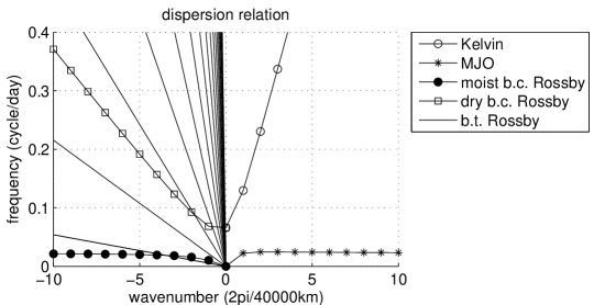
First, in the baroclinic system (22) (with FW=0subscript𝐹𝑊0{\vec{F}_{\vec{W}}}=\vec{0}), the components of vector W=(K,R,Q,A,l(2),q(2))𝑊𝐾𝑅𝑄𝐴superscript𝑙2superscript𝑞2\vec{W}=(K,R,Q,A,{l^{(2)}},{q^{(2)}}) can be separated into two groups: (K,R,Q,A)𝐾𝑅𝑄𝐴(K,R,Q,A) and (l(2),q(2))superscript𝑙2superscript𝑞2({l^{(2)}},{q^{(2)}}). The KRQA system is closed (as can be seen in its explicit formulation in Appendix C), and its four eigenmodes have been described previously [18]: dry Kelvin, MJO, moist Rossby and dry Rossby, as shown in figure 1. In brief, the dry Kelvin wave is a fast eastward-propagating wave; the MJO is a slow east-propagating wave; and the moist and dry baroclinic Rossby waves are slow and fast westward-propagating waves, respectively. In addition to the KRQA system, l(2)superscript𝑙2{l^{(2)}} satisfies an independent (decoupled) equation, and q(2)superscript𝑞2{q^{(2)}} is slaved to (K,R,Q,A)𝐾𝑅𝑄𝐴(K,R,Q,A) and l(2)superscript𝑙2{l^{(2)}} (see the explicit formulation in Appendix C). Therefore the eigenmodes from the KRQA system of [18] are not affected by the additional two variables l(2)superscript𝑙2{l^{(2)}} and q(2)superscript𝑞2{q^{(2)}}. Notice that the baroclinic Rossby and Kelvin waves in this model are dry equatorial waves, not convectively coupled equatorial waves (CCEWs) [7]. The model here is a planetary-scale model that does not explicitly resolve CCEWs, which occur mainly on smaller, synoptic scales. Nevertheless, one would expect similar wave interactions to hold for CCEWs, due to the similar structures of dry and convectively coupled waves, if a model were used that resolved such synoptic-scale convectively coupled waves.
Refer to caption
Figure 1: Dispersion relation of the KRQA system and barotropic wind with different meridional wavelengths.

Second, for the barotropic system (19a), the dispersion relation is written explicitly as

ωT(k)=kL2.subscript𝜔T𝑘𝑘superscript𝐿2{\omega_{\text{T}}}(k)=-\frac{k}{L^{2}}. (23)

The above formula implies that barotropic Rossby waves travel faster for smaller meridional wavenumber L𝐿L or, equivalently, longer meridional wavelength Y𝑌Y. In figure 1, barotropic dispersion relation are shown with different meridional wave numbers.

6 The reduced asymptotic models

In this section, the following reduced asymptotic model is derived and its basic features are described:

T2β+id1βj11βj112+id2β+id3α1α2=0,subscriptsubscript𝑇2𝛽𝑖subscript𝑑1subscript𝛽subscript𝑗11superscriptsubscript𝛽subscript𝑗11absent2𝑖subscript𝑑2𝛽𝑖subscript𝑑3superscriptsubscript𝛼1superscriptsubscript𝛼20\displaystyle-\partial_{T_{2}}\beta{\color[rgb]{1,1,1}+id_{1}\beta_{j_{1}1}\beta_{j_{1}1}^{*2}}+id_{2}\beta+id_{3}\alpha_{1}^{*}\alpha_{2}^{*}=0, (24a)
T2α1+id4α12α1+id5α1+id6βα2=0,subscriptsubscript𝑇2subscript𝛼1𝑖subscript𝑑4superscriptsubscript𝛼12superscriptsubscript𝛼1𝑖subscript𝑑5subscript𝛼1𝑖subscript𝑑6superscript𝛽superscriptsubscript𝛼20\displaystyle-\partial_{T_{2}}{\alpha_{1}}+id_{4}{\alpha_{1}}^{2}\alpha_{1}^{*}+id_{5}{\alpha_{1}}+id_{6}\beta^{*}\alpha_{2}^{*}=0, (24b)
T2α2+id7α22α2+id8α2+id9βα1=0,subscriptsubscript𝑇2subscript𝛼2𝑖subscript𝑑7superscriptsubscript𝛼22superscriptsubscript𝛼2𝑖subscript𝑑8subscript𝛼2𝑖subscript𝑑9superscript𝛽superscriptsubscript𝛼10\displaystyle-\partial_{T_{2}}{\alpha_{2}}+id_{7}{\alpha_{2}}^{2}\alpha_{2}^{*}+id_{8}{\alpha_{2}}+id_{9}\beta^{*}\alpha_{1}^{*}=0, (24c)

where the coefficients djsubscript𝑑𝑗d_{j} are all real numbers. This is a system of ODEs for three-wave resonance, where β𝛽\beta is the complex amplitude of the barotropic Rossby waves, and α1subscript𝛼1\alpha_{1} and α2subscript𝛼2\alpha_{2} are the complex amplitudes of two baroclinic waves. The superscript * stands for complex conjugate. For the applications of importance here, one of the α𝛼\alphas will correspond to the MJO, and this ODE system describes its interaction with the other waves, with an aim toward MJO initiation and termination.

In brief, the terms in (24) fall into three groups that are linked to different features in the full 2D model (1): the cubic terms are associated with the nonlinear q𝑞q-a𝑎a interactions; the linear terms come from dispersive terms; the quadratic terms rise from the nonlinear baroclinic-barotropic interactions. Here, in particular, the cubic self-interaction terms are a novel feature that are not typically found in three-wave resonance ODEs, and they arise here from the effects of water vapor q𝑞q and convective activity a𝑎a.

In the remainder of this section, two basic properties of the system are described – energy conservation and a family of equilibrium points – and the derivation is sketched, with details of the derivation shown in Appendix D.

6.1 Energy conservation

The ODE system (24) satisfies the following energy conservation principle:

T2(ββ+α1α1+α2α2)=0.subscript𝑇2𝛽superscript𝛽subscript𝛼1superscriptsubscript𝛼1subscript𝛼2superscriptsubscript𝛼20\frac{\partial}{\partial T_{2}}(\beta\beta^{*}+{\alpha_{1}}{\alpha_{1}}^{*}+{\alpha_{2}}{\alpha_{2}}^{*})=0. (25)

This conserved quantity is a consequence that all coefficients are pure imaginary, and in particular, that

d3+d6+d9=0,subscript𝑑3subscript𝑑6subscript𝑑90d_{3}+d_{6}+d_{9}=0, (26)

which is a key component for energy conservation in three-wave interaction equations [13].

6.2 Equilibium points in ODE system

In addition to the trivial equilibrium point of (24) where β=α1=α2=0𝛽subscript𝛼1subscript𝛼20\beta=\alpha_{1}=\alpha_{2}=0, a family of nontrivial equilibrium points also exists:

|α1|2superscriptsubscript𝛼12\displaystyle|{\alpha_{1}}|^{2} =d22d5d7+d2d3d6d8d32d6d9d22d4d7absentsuperscriptsubscript𝑑22subscript𝑑5subscript𝑑7subscript𝑑2subscript𝑑3subscript𝑑6subscript𝑑8superscriptsubscript𝑑32subscript𝑑6subscript𝑑9superscriptsubscript𝑑22subscript𝑑4subscript𝑑7\displaystyle=\frac{d_{2}^{2}d_{5}d_{7}+d_{2}d_{3}d_{6}d_{8}}{d_{3}^{2}d_{6}d_{9}-d_{2}^{2}d_{4}d_{7}} (27a)
|α2|2superscriptsubscript𝛼22\displaystyle|{\alpha_{2}}|^{2} =d22d4d8+d2d3d9d5d32d6d9d22d4d7absentsuperscriptsubscript𝑑22subscript𝑑4subscript𝑑8subscript𝑑2subscript𝑑3subscript𝑑9subscript𝑑5superscriptsubscript𝑑32subscript𝑑6subscript𝑑9superscriptsubscript𝑑22subscript𝑑4subscript𝑑7\displaystyle=\frac{d_{2}^{2}d_{4}d_{8}+d_{2}d_{3}d_{9}d_{5}}{d_{3}^{2}d_{6}d_{9}-d_{2}^{2}d_{4}d_{7}} (27b)
β𝛽\displaystyle\beta =d3d2α1α2absentsubscript𝑑3subscript𝑑2superscriptsubscript𝛼1superscriptsubscript𝛼2\displaystyle=-\frac{d_{3}}{d_{2}}{\alpha_{1}}^{*}{\alpha_{2}}^{*} (27c)

Two examples for the nontrivial equilibrium points are considered here:

|α1|0.24,|α2|0.20,|β|0.0033 for case MRB,formulae-sequencesubscript𝛼10.24formulae-sequencesubscript𝛼20.20𝛽0.0033 for case MRB,\displaystyle|{\alpha_{1}}|\approx 0.24,\quad|{\alpha_{2}}|\approx 0.20,\quad|\beta|\approx 0.0033\text{ for case MRB,} (28a)
|α1|2.4,|α2|7.5,|β|0.34 for case MKB.formulae-sequencesubscript𝛼12.4formulae-sequencesubscript𝛼27.5𝛽0.34 for case MKB.\displaystyle|{\alpha_{1}}|\approx 2.4,\quad|{\alpha_{2}}|\approx 7.5,\quad|\beta|\approx 0.34\text{ for case MKB.} (28b)

The MRB and MKB are cases for different resonance triads. For MRB, the M stands for MJO, the R stands for equatorial Rossby wave, and the B stands for barotropic Rossby wave; and for MKB, the M and B are the same, and the K stands for equatorial Kelvin wave. These two cases are further discussed in Section 8 (although the simulations in Section 8 are not set up to illustrate the dynamics near these nontrivial equilibrium points).

In a linear stability analysis (not shown), the system (8) is neutrally stable when linearized around the trivial equilibrium point of 00\vec{0}. On the other hand, when linearized around the two examples of the nontrivial equilibrium points, the system is unstable. It would be interesting to further explore these cases and their physical interpretations in the future.

6.3 Derivation

The derivation of (24) starts by assuming a leading order barotropic component of the form

B1=1ETβ(T1,T2)eiθT+C.C.,subscript𝐵11subscript𝐸T𝛽subscript𝑇1subscript𝑇2superscript𝑒𝑖subscript𝜃TC.C.B_{1}=\frac{1}{\sqrt{E_{\text{T}}}}{\beta}(T_{1},T_{2})e^{i{\theta_{\text{T}}}}+\text{C.C.}, (29)

where θT=kTx+ωTtsubscript𝜃Tsubscript𝑘Tsuperscript𝑥subscript𝜔Tsuperscript𝑡{\theta_{\text{T}}}={k_{\text{T}}}x^{\prime}+{\omega_{\text{T}}}t^{\prime}, and ETsubscript𝐸TE_{\text{T}} is the barotropic energy unit

ET=2YL2,subscript𝐸T2𝑌superscript𝐿2E_{\text{T}}=2YL^{2},

and leading order baroclinic variables of the form

W1subscript𝑊1\displaystyle\vec{W}_{1} =α1eiθ1r1+α2eiθ2r2+C.C.,absentsubscript𝛼1superscript𝑒𝑖subscript𝜃1subscript𝑟1subscript𝛼2superscript𝑒𝑖subscript𝜃2subscript𝑟2C.C.\displaystyle={\alpha_{1}}e^{i{\theta_{1}}}\vec{r}_{1}+{\alpha_{2}}e^{i{\theta_{2}}}\vec{r}_{2}+\text{C.C.}, (30)

where θj=kjx+ωjtsubscript𝜃𝑗subscript𝑘𝑗superscript𝑥subscript𝜔𝑗superscript𝑡\theta_{j}=k_{j}x^{\prime}+\omega_{j}t^{\prime}, and r𝑟\vec{r} represents a right eigenvector of the linear system with components

rj=(K^1,j,R^1,j,Q^1,j,A^1,j,l(2)^1,j,q(2)^1,j),j=1,2.formulae-sequencesubscript𝑟𝑗subscript^𝐾1𝑗subscript^𝑅1𝑗subscript^𝑄1𝑗subscript^𝐴1𝑗subscript^superscript𝑙21𝑗subscript^superscript𝑞21𝑗𝑗12\vec{r}_{j}=(\hat{K}_{1,j},\hat{R}_{1,j},\hat{Q}_{1,j},\hat{A}_{1,j},\hat{{l^{(2)}}}_{1,j},\hat{{q^{(2)}}}_{1,j}),\quad j=1,2.

Here the arbitrary complex phase factor of each eigenvector is chosen so that K^1,jsubscript^𝐾1𝑗\hat{K}_{1,j} is a real number, and the eigenvectors rjsubscript𝑟𝑗\vec{r}_{j} are normalized with respect to the energy as

Ej=rjrj=1,j=1,2,formulae-sequencesubscript𝐸𝑗superscriptsubscript𝑟𝑗subscript𝑟𝑗1𝑗12\displaystyle E_{j}=\vec{r}_{j}^{{\dagger}}\mathcal{H}\vec{r}_{j}=1,\quad j=1,2, (31)

where \mathcal{H} is the Hessian matrix of the conserved energy for the linear baroclinic system.

Next, two auxiliary problems must be solved, (56) and (57) of Appendix C, one for each of the two long time scales, T1=δtsubscript𝑇1𝛿superscript𝑡T_{1}=\delta t^{\prime} and T2=δ2tsubscript𝑇2superscript𝛿2superscript𝑡T_{2}=\delta^{2}t^{\prime}. The solution of the auxiliary problems is the key step in the method of multiscale asymptotics in order to suppress secular growth and guarantee a consistent asymptotic expansion of the variables [13]. As part of the second auxiliary problem, the three waves must satisfy the following resonance conditions:

k1+k2+kTsubscript𝑘1subscript𝑘2subscript𝑘T\displaystyle{k_{1}}+{k_{2}}+{k_{\text{T}}} =0,absent0\displaystyle=0, (32a)
ω1+ω2+ωTsubscript𝜔1subscript𝜔2subscript𝜔T\displaystyle{\omega_{1}}+{\omega_{2}}+{\omega_{\text{T}}} =0.absent0\displaystyle=0. (32b)

Further details of derivation are presented in Appendix D.

7 Validation study: the wavenumber–2 MJO mode

In this section, a special case is considered in order to explore the time scales of validity of the ODE system in (24). If only a single baroclinic mode is considered, without a barotropic mode, the ODE system in (24) becomes a single ODE:

T2α1+id4α12α1+id5α1=0.subscriptsubscript𝑇2subscript𝛼1𝑖subscript𝑑4superscriptsubscript𝛼12superscriptsubscript𝛼1𝑖subscript𝑑5subscript𝛼10-\partial_{T_{2}}{\alpha_{1}}+id_{4}{\alpha_{1}}^{2}{\alpha_{1}}^{*}+id_{5}{\alpha_{1}}=0. (33)

The energy conservation of this single mode then takes the form

T2(α1α1)=0.subscript𝑇2subscript𝛼1superscriptsubscript𝛼10\frac{\partial}{\partial T_{2}}({\alpha_{1}}{\alpha_{1}}^{*})=0. (34)

This special case can then be compared against numerical solutions that have been presented previously elsewhere [19], which will be regarded as the ‘true’ solution here. The specific case chosen is Case U2 of [19], which has a wavenumber-2 MJO eigenmode as the initial condition for a nonlinear simulation.

A few technical details for consistency with [19] are the following. The coefficient c1subscript𝑐1c_{1} in (36) is taken to be 111 for consistency with the equation At=ΓQAsubscript𝐴𝑡Γ𝑄𝐴A_{t}=\Gamma QA used in [19]. Also, since the model of [19] does not include the dispersive effects of v(1)superscript𝑣1{v^{(1)}} (although it does include other dispersive effects), the coefficient d5subscript𝑑5d_{5} in the ODE system (33) is set to 0. As in [19], here the computational domain is [0,X]0𝑋[0,X], where X=40,000𝑋40000X=40,000 km in the circumference of Earth at the equator.

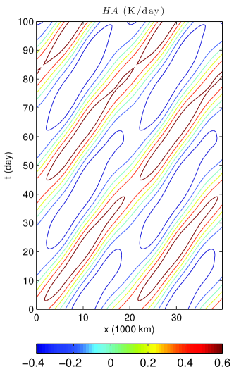
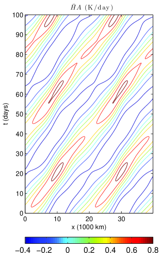
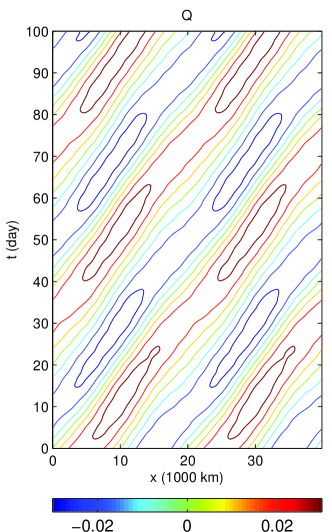
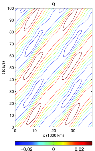
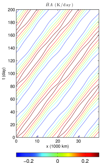
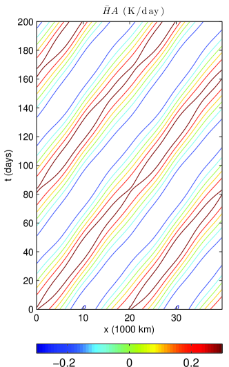
For the validation study, three different values of δ𝛿\delta are chosen: δ=0.1𝛿0.1\delta=\sqrt{0.1}, 0.1/20.12\sqrt{0.1}/2 and 0.1/40.14\sqrt{0.1}/4, corresponding to three different RCE states: δ2a¯=superscript𝛿2¯𝑎absent\delta^{2}{\bar{a}}= 0.1, 0.025 and 0.00625. The solutions are evolved out to times 100, 200, and 400 days respectively, matching the long wave assumption. Table 4 shows the relative error between the asymptotic solution and the ‘true’ solution. The relative error decreases by a factor of 2 as δ𝛿\delta is decreased by a factor of 2, indicating a relative error of O(δ)𝑂𝛿O(\delta), suggesting an absolute error of O(δ3)𝑂superscript𝛿3O(\delta^{3}) and a true solution with magnitude of O(δ2)𝑂superscript𝛿2O(\delta^{2}). Figures 2 and 3 show comparisons between the asymptotic solutions and numerical (‘true’) solutions for δ=0.1𝛿0.1\delta=\sqrt{0.1} and 0.1/20.12\sqrt{0.1}/2 (with δ=0.1/4𝛿0.14\delta=\sqrt{0.1}/4 not shown since it is indistinguishable from the ‘true’ solution). In Figure 2, the agreement is good out to 100 days, although some of the peaks in convective activity H¯A¯𝐻𝐴\bar{H}A are not captured by the asymptotic solution. In Figure 3, the agreement is excellent out to 200 days.

As a further validity test of the asymptotic model, the same comparisons have been repeated (not shown) with the addition of the second order corrections. More specifically, whereas the asymptotic solution Wasymsubscript𝑊asym\vec{W}_{\text{asym}} in Table 4 was defined as Wasym=δ2W1subscript𝑊asymsuperscript𝛿2subscript𝑊1\vec{W}_{\text{asym}}=\delta^{2}\vec{W}_{1}, the comparisons have been repeated using Wasym=δ2W1+δ3W2subscript𝑊asymsuperscript𝛿2subscript𝑊1superscript𝛿3subscript𝑊2\vec{W}_{\text{asym}}=\delta^{2}\vec{W}_{1}+\delta^{3}\vec{W}_{2}, where the second order correction W2subscript𝑊2\vec{W}_{2} is described in more detail in Appendix C and D. In these new tests, the values of Table 4 change to 0.2685, 0.0627, 0.0183. These values show a decrease in relative error of a factor of 4 as δ𝛿\delta is decreased by a factor of 2, indicating a relative error of O(δ2)𝑂superscript𝛿2O(\delta^{2}), in line with an absolute error of O(δ4O(\delta^{4}) and a true solution with magnitude of O(δ2)𝑂superscript𝛿2O(\delta^{2}).

In summary, the asymptotic solutions have significant accuracy on time scales of 100 days or longer, which are roughly the time scales for application to tropical–extratropical interactions and MJO initiation and termination.

δ2a¯=superscript𝛿2¯𝑎absent\delta^{2}{\bar{a}}=0.1 at 100100100 day δ2a¯=superscript𝛿2¯𝑎absent\delta^{2}{\bar{a}}=0.025 at 200 day δ2a¯=superscript𝛿2¯𝑎absent\delta^{2}{\bar{a}}=0.00625 at 400 day
WasymWn/Wnnormsubscript𝑊asymsubscript𝑊nnormsubscript𝑊n\|\vec{W}_{\text{asym}}-\vec{W}_{\text{n}}\|/\|\vec{W}_{\text{n}}\| 0.3890 0.1657 0.0770
Table 4: The relative difference between numerical solution Wnsubscript𝑊𝑛\vec{W}_{n} (regarded as the ‘true’ solution here) and the asymptotic solution (Wasymsubscript𝑊asym\vec{W}_{\text{asym}}) whose amplitude αj1(T2)subscript𝛼subscript𝑗1subscript𝑇2\alpha_{j_{1}}(T_{2}) is governed by the ODE (33). Three different values of δ𝛿\delta are considered along with three different corresponding times.
Refer to caption
Refer to caption
Refer to caption
Refer to caption
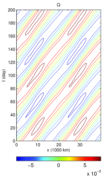
Figure 2: Comparisons between asymptotic solutions (left) and numerical (‘true’) solutions (right) for A¯=0.1¯𝐴0.1{\bar{A}}=0.1 for the case of a wavenumber-2 MJO mode. The convective activity H¯A¯𝐻𝐴\bar{H}A (top) and the water vapor Q𝑄Q (bottom) are shown as functions of x𝑥x and t𝑡t.
Refer to caption
Refer to caption
Refer to caption
Refer to caption
Figure 3: Comparisons between asymptotic solutions (left) and numerical (‘true’) solutions (right) for A¯=0.025¯𝐴0.025{\bar{A}}=0.025 for the case of a wavenumber-2 MJO mode. The convective activity H¯A¯𝐻𝐴\bar{H}A (top) and the water vapor Q𝑄Q (bottom) are shown as functions of x𝑥x and t𝑡t.

8 Three–wave interactions

Here two types of three-wave interactions are considered as shown in figure 4:

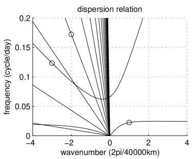
(1): MJO–dry baroclinic Rossby–barotropic Rossby waves (MRB)ωMJO(1)+ωR(3)+ωT,Y2,000 km(2)=0(2): MJO–dry Kelvin–barotropic Rossby waves (MKB)ωMJO(3)+ωK(2)+ωT,Y3,000 km(1)=0\begin{array}[]{ll}\text{(1):}&\text{ MJO--dry baroclinic Rossby--barotropic Rossby waves (MRB)}\\ &{\omega_{\text{MJO}}}(1)+{\omega_{\text{R}}}(-3)+{\omega_{\text{T}}}_{,Y\approx\text{2,000~{}km}}(2)=0\\ &\\ \text{(2):}&\text{ MJO--dry Kelvin--barotropic Rossby waves (MKB)}\\ &{\omega_{\text{MJO}}}(-3)+{\omega_{\text{K}}}(2)+{\omega_{\text{T}}}_{,Y\approx\text{3,000~{}km}}(1)=0\end{array} (35)

For the acronym MRB, the M stands for MJO, the R stands for equatorial Rossby wave, and the B stands for barotropic Rossby wave; and for MKB, the M and B are the same, and the K stands for equatorial Kelvin wave. The meridional wavelength 2Y2𝑌2Y of the barotropic Rossby wave is chosen so that the resonance conditions (32) are exactly satisfied. The numerical results here are focused on the ODE system (24), with wave amplitudes β𝛽\beta, α1subscript𝛼1{\alpha_{1}}, and α2subscript𝛼2{\alpha_{2}}, where the energy exchange between three waves is of the most interest. The coefficients in (24) for the two cases are in table 5. The RCE a¯¯𝑎{\bar{a}} is chosen to be a¯=0.1¯𝑎0.1{\bar{a}}=0.1 so that the small parameter δ=0.1𝛿0.1\delta=\sqrt{0.1}.

d2subscript𝑑2d_{2} d3subscript𝑑3d_{3} d4subscript𝑑4d_{4} d5subscript𝑑5d_{5} d6subscript𝑑6d_{6} d7subscript𝑑7d_{7} d8subscript𝑑8d_{8} d9subscript𝑑9d_{9}
MRB 0.450.45-0.45 8.3e8.3𝑒-8.3e-333 5.2e5.2𝑒-5.2e-222 1.7e1.7𝑒1.7e-333 0.280.28-0.28 2.4e2.4𝑒-2.4e-222 1.371.371.37 0.290.290.29
MKB 0.450.450.45 3.2e3.2𝑒-3.2e-222 0.110.11-0.11 6.0e6.0𝑒6.0e-333 0.110.110.11 7.8e7.8𝑒7.8e-333 8.5e8.5𝑒-8.5e-777 7.6e7.6𝑒-7.6e-222
Table 5: Coefficients djsubscript𝑑𝑗d_{j} for the 3-wave interaction ODEs (24) for two cases: the MJO, dry baroclinic Rossby, and barotropic Rossby wave interactions (MRB) (top row) and the MJO, dry Kelvin, and barotropic Rossby wave interactions (MKB) (bottom row).

8.1 MJO–dry baroclinic Rossby–barotropic Rossby waves (MRB)

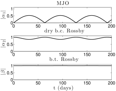
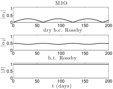
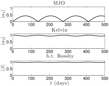
In this case, α1subscript𝛼1{\alpha_{1}} and α2subscript𝛼2{\alpha_{2}} are the amplitudes for the MJO and dry baroclinic Rossby waves, respectively. To consider MJO initiation, α1subscript𝛼1{\alpha_{1}} is set to be zero for the initial condition in the ODE, and the other waves have amplitudes of |α2(t=0)|=|β(t=0)|=1subscriptsubscript𝛼2𝑡0subscript𝛽𝑡01|{\alpha_{2}}_{(t=0)}|=|\beta_{(t=0)}|=1. The results of the numerical simulation are shown in Figure 5. The waves exchange energy periodically, with period of about 60 days, roughly the time scale for MJO initiation and termination in nature. At early times, the MJO amplitude grows (i.e., the MJO initiates) by extracting energy from the other two waves, mainly from the dry baroclinic Rossby wave. Termination of the MJO then follows from a transfer of energy back to the dry baroclinic Rossby wave.

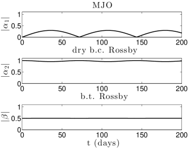
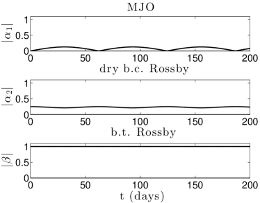
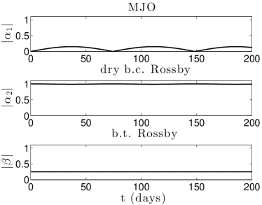
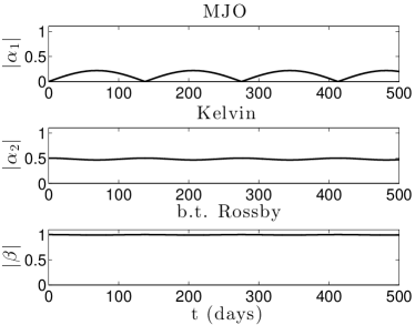
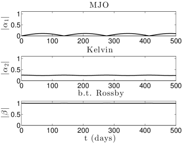
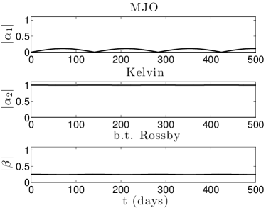
To explore the sensitivity of these results, different initial conditions are chosen, and the results are in figure 6. The initial amplitudes for baroclinic Rossby wave and barotropic Rossby waves are (a) |α2(t=0)|=0.5subscriptsubscript𝛼2𝑡00.5|{\alpha_{2}}_{(t=0)}|=0.5,|β(t=0)|=1subscript𝛽𝑡01|\beta_{(t=0)}|=1; (b) |α2(t=0)|=1subscriptsubscript𝛼2𝑡01|{\alpha_{2}}_{(t=0)}|=1, |β(t=0)|=0.5subscript𝛽𝑡00.5|\beta_{(t=0)}|=0.5; (c) |α2(t=0)|=0.25subscriptsubscript𝛼2𝑡00.25|{\alpha_{2}}_{(t=0)}|=0.25, |β(t=0)|=1subscript𝛽𝑡01|\beta_{(t=0)}|=1; (d) |α2(t=0)|=1subscriptsubscript𝛼2𝑡01|{\alpha_{2}}_{(t=0)}|=1, |β(t=0)|=0.25subscript𝛽𝑡00.25|\beta_{(t=0)}|=0.25. The simulations are performed with different initial phases of α2subscript𝛼2{\alpha_{2}} and β𝛽\beta, but this has no effect on the evolution of the amplitudes. In the simulations in Figure 6, it can be seen that the amount of energy extracted by the MJO varies roughly proportionally to the amount of energy present initially in the dry baroclinic Rossby wave and barotropic Rossby wave. On the other hand, the time scale for the energy exchange changes very little among these cases. In all cases, the energy of the barotropic Rossby wave stays essentially constant and is not transferred to the MJO. These results indicate that the eventual strength of the MJO depends on the amplitude of the barotropic Rossby waves, but the MJO acquires its energy from the baroclinic rather than barotropic Rossby waves.

8.2 MJO–dry Kelvin–barotropic Rossby waves (MKB)

In this case, α1subscript𝛼1{\alpha_{1}} and α2subscript𝛼2{\alpha_{2}} are the amplitudes for the MJO and dry baroclinic Kelvin waves, respectively. Again considering MJO initiation, the initial conditions are α1=0subscript𝛼10{\alpha_{1}}=0 and |α2(t=0)|=|β(t=0)|=1subscriptsubscript𝛼2𝑡0subscript𝛽𝑡01|{\alpha_{2}}_{(t=0)}|=|\beta_{(t=0)}|=1, and the results are shown in Figure 7. While the solution is similar in character to the MRB case, two main differences can be seen. First, the temporal period of roughly 120 days is twice that of the MRB case but still within the range of time scales for MJO initiation and termination in nature. Secondly, both the dry Kelvin wave and the barotropic Rossby waves contribute to the growth of MJO, although the energy exchange with the barotropic Rossby wave is somewhat small.

Finally, the sensitivity of the results is illustrated in Figure 8, which shows numerical results with different initial amplitudes. As in the MRB case, the amount of energy extracted by the MJO varies roughly proportionally to the amount of energy present initially in the other two modes.

Refer to caption
Refer to caption
Figure 4: Resonance condition for three-wave interactions, where circles indicate the particular wave numbers and frequencies that leads to resonances. Left: MJO, Kelvin and barotropic Rossby wave; right: MJO, Rossby and barotropic Rossby wave.
Refer to caption
Figure 5: MJO–Rossby–barotropic Rossby wave interactions. Initial condition: α1subscript𝛼1{\alpha_{1}} = 0, |α2(t=0)|=|β(t=0)|=1subscriptsubscript𝛼2𝑡0subscript𝛽𝑡01|{\alpha_{2}}_{(t=0)}|=|\beta_{(t=0)}|=1.
Refer to caption
Refer to caption

 Refer to caption Refer to caption

Figure 6: MJO–Rossby–barotropic Rossby wave interactions. Initial condition: α1subscript𝛼1{\alpha_{1}} = 0. (a) |α2(t=0)|=0.5subscriptsubscript𝛼2𝑡00.5|{\alpha_{2}}_{(t=0)}|=0.5,|β(t=0)|=1subscript𝛽𝑡01|\beta_{(t=0)}|=1; (b) |α2(t=0)|=1subscriptsubscript𝛼2𝑡01|{\alpha_{2}}_{(t=0)}|=1, |β(t=0)|=0.5subscript𝛽𝑡00.5|\beta_{(t=0)}|=0.5; (c) |α2(t=0)|=0.25subscriptsubscript𝛼2𝑡00.25|{\alpha_{2}}_{(t=0)}|=0.25, |β(t=0)|=1subscript𝛽𝑡01|\beta_{(t=0)}|=1; (d) |α2(t=0)|=1subscriptsubscript𝛼2𝑡01|{\alpha_{2}}_{(t=0)}|=1, |β(t=0)|=0.25subscript𝛽𝑡00.25|\beta_{(t=0)}|=0.25.
Refer to caption
Figure 7: MJO–Kelvin–barotropic Rossby wave interactions. Initial condition: α1subscript𝛼1{\alpha_{1}} = 0, |α2(t=0)|=|β(t=0)|=1subscriptsubscript𝛼2𝑡0subscript𝛽𝑡01|{\alpha_{2}}_{(t=0)}|=|\beta_{(t=0)}|=1.
Refer to caption
Refer to caption

 Refer to caption Refer to caption

Figure 8: MJO–Kelvin–barotropic Rossby wave interactions. Initial condition: α1subscript𝛼1{\alpha_{1}} = 0. (a) |α2(t=0)|=0.5subscriptsubscript𝛼2𝑡00.5|{\alpha_{2}}_{(t=0)}|=0.5,|β(t=0)|=1subscript𝛽𝑡01|\beta_{(t=0)}|=1; (b) |α2(t=0)|=1subscriptsubscript𝛼2𝑡01|{\alpha_{2}}_{(t=0)}|=1, |β(t=0)|=0.5subscript𝛽𝑡00.5|\beta_{(t=0)}|=0.5; (c) |α2(t=0)|=0.25subscriptsubscript𝛼2𝑡00.25|{\alpha_{2}}_{(t=0)}|=0.25, |β(t=0)|=1subscript𝛽𝑡01|\beta_{(t=0)}|=1; (d) |α2(t=0)|=1subscriptsubscript𝛼2𝑡01|{\alpha_{2}}_{(t=0)}|=1, |β(t=0)|=0.25subscript𝛽𝑡00.25|\beta_{(t=0)}|=0.25.

9 Summary and conclusions

A new model has been proposed here to describe MJO initiation and termination and tropical-extratropical interactions. The model involves the integration of the barotropic and equatorial baroclinic modes together with moisture and convective activity envelope, all interacting together with a conserved energy. Using the method of multiscale asymptotics with multiple time scales, simplified asymptotic equations were derived for the resonant interaction of tropical and extratropical waves. The simplified model is an ODE system for wave amplitudes, including quadratic nonlinearity as in many traditional three-wave-resonance equations, and also including cubic self-interaction terms that arise from nonlinear interactions of water vapor and convective activity.

Example simulations of the ODE system are shown to illustrate some cases of MJO initiation. In this model, the MJO is shown to initiate mainly by extracting energy from either the dry Kelvin wave or the dry equatorial baroclinic Rossy wave. While the MJO extracts a smaller amount of energy from the barotropic Rossby waves, the barotropic Rossby waves are essential for MJO initiation, and the strength of the ensuing MJO depends on the strength of the barotropic Rossby waves present. In this way, the barotropic Rossby wave acts as a catalyst for the interaction of the other two waves. In other scenarios, it is possible that the barotropic Rossby wave may lose or gain energy through wave interactions if more realistic setups are used. For example, (i) zonally varying climatological mean state, and (ii) shear could affect the interaction mechanisms. In the future, it would also be interesting to include the effects of additional meridional modes that are asymmetric with respect to the equator in order to model the Boreal summer MJO and monsoon intraseasonal variability [35]. The authors are currently pursuing these issues and will report on them in the near future.

The simplified models suggest specific classes of waves that could be investigated in observations among the plethora of possible waves and wave interaction scenarios. More specifically, one can imagine wave interactions among many different types of waves. Here, in this paper, we have identified specific classes of three-wave interactions involving the MJO. For example, one class involved a wavenumber-1 MJO, wavenumber-3 dry baroclinic Rossby wave, and wavenumber-2 barotropic Rossby wave. It would be interesting to identify this specific class of waves in observational data and investigate their interactions. Such an investigation and comparison with the model could be challenging for many reasons; for example, as described above, the mean state of the model version here does not include a zonally varying climatological mean state nor wind shear, which may influence the wave interactions.

Appendix A The explicit formulation of the meridional truncated system

Applying the meridional truncation of (14) to the long-wave-scaled system of (6) leads to the truncated system:

L2YBtYBx=𝒞T+δ2(YBxxt+𝒟T)superscript𝐿2𝑌subscript𝐵superscript𝑡𝑌subscript𝐵superscript𝑥subscript𝒞Tsuperscript𝛿2𝑌subscript𝐵superscript𝑥superscript𝑥superscript𝑡subscript𝒟T\displaystyle L^{2}YB_{t^{\prime}}-YB_{x^{\prime}}={\mathcal{C}}_{\text{T}}+\delta^{2}\left(YB_{x^{\prime}x^{\prime}t^{\prime}}+{\mathcal{D}}_{\text{T}}\right) (36a)
l(0)tl(0)x+v(1)+12δH¯a(0)=𝒞l(0)subscriptsuperscript𝑙0superscript𝑡subscriptsuperscript𝑙0superscript𝑥superscript𝑣112𝛿¯𝐻superscript𝑎0subscript𝒞superscript𝑙0\displaystyle{l^{(0)}}_{t^{\prime}}-{l^{(0)}}_{x^{\prime}}+{v^{(1)}}+\frac{1}{\sqrt{2}}\delta{\bar{H}}{a^{(0)}}={\mathcal{C}}_{{l^{(0)}}} (36b)
l(2)tl(2)x=𝒞l(2)subscriptsuperscript𝑙2𝑡subscriptsuperscript𝑙2𝑥subscript𝒞superscript𝑙2\displaystyle{l^{(2)}}_{t}-{l^{(2)}}_{x}={\mathcal{C}}_{{l^{(2)}}} (36c)
r(0)t+r(0)x+12δH¯a(0)=𝒞r(0)subscriptsuperscript𝑟0superscript𝑡subscriptsuperscript𝑟0superscript𝑥12𝛿¯𝐻superscript𝑎0subscript𝒞superscript𝑟0\displaystyle{r^{(0)}}_{t^{\prime}}+{r^{(0)}}_{x^{\prime}}+\frac{1}{\sqrt{2}}\delta{\bar{H}}{a^{(0)}}={\mathcal{C}}_{{r^{(0)}}} (36d)
r(2)t+r(2)x2v(1)=𝒞r(2)subscriptsuperscript𝑟2superscript𝑡subscriptsuperscript𝑟2superscript𝑥2superscriptsuperscript𝑣1subscript𝒞superscript𝑟2\displaystyle{r^{(2)}}_{t^{\prime}}+{r^{(2)}}_{x^{\prime}}-\sqrt{2}{v^{(1)}}^{\prime}={\mathcal{C}}_{{r^{(2)}}} (36e)
2r(2)l(0)=δ2(v(1)t+𝒟v(1))2superscript𝑟2superscript𝑙0superscript𝛿2subscriptsuperscriptsuperscript𝑣1superscript𝑡subscript𝒟superscript𝑣1\displaystyle\sqrt{2}{r^{(2)}}-{l^{(0)}}=\delta^{2}(-{v^{(1)}}^{\prime}_{t^{\prime}}+{\mathcal{D}}_{{v^{(1)}}}) (36f)
q(0)t+Q~2(r(0)xl(0)x)+Q~2v(1)+δH¯a(0)=𝒞q(0)subscriptsuperscript𝑞0superscript𝑡~𝑄2subscriptsuperscript𝑟0superscript𝑥subscriptsuperscript𝑙0superscript𝑥~𝑄2superscriptsuperscript𝑣1𝛿¯𝐻superscript𝑎0subscript𝒞superscript𝑞0\displaystyle{q^{(0)}}_{t^{\prime}}+\frac{{\tilde{Q}}}{\sqrt{2}}({r^{(0)}}_{x^{\prime}}-{l^{(0)}}_{x^{\prime}})+\frac{{\tilde{Q}}}{\sqrt{2}}{v^{(1)}}^{\prime}+\delta{\bar{H}}{a^{(0)}}={\mathcal{C}}_{{q^{(0)}}} (36g)
q(2)t+Q~2(r(2)xl(2)x)Q~v(1)=𝒞q(2)subscriptsuperscript𝑞2superscript𝑡~𝑄2subscriptsuperscript𝑟2superscript𝑥subscriptsuperscript𝑙2superscript𝑥~𝑄superscriptsuperscript𝑣1subscript𝒞superscript𝑞2\displaystyle{q^{(2)}}_{t^{\prime}}+\frac{{\tilde{Q}}}{\sqrt{2}}({r^{(2)}}_{x^{\prime}}-{l^{(2)}}_{x^{\prime}})-{\tilde{Q}}{v^{(1)}}^{\prime}={\mathcal{C}}_{{q^{(2)}}} (36h)
a(0)tΓa¯q(0)=c1Γa(0)q(0)+c10Γa(0)q(2)subscriptsuperscript𝑎0superscript𝑡Γ¯𝑎superscript𝑞0subscript𝑐1Γsuperscript𝑎0superscript𝑞0subscript𝑐10Γsuperscript𝑎0superscript𝑞2\displaystyle{a^{(0)}}_{t^{\prime}}-\Gamma{\bar{a}}{q^{(0)}}=c_{1}\Gamma{a^{(0)}}{q^{(0)}}+c_{10}\Gamma{a^{(0)}}{q^{(2)}} (36i)

which is written in vector form in (19). Here 𝒞𝒞{\mathcal{C}} and 𝒟𝒟{\mathcal{D}} are bilinear terms at different orders:

𝒞T=c22(r(0)l(0))x2c32[(r(0)l(0))(r(2)l(2))]xsubscript𝒞Tsubscript𝑐22subscriptsuperscriptsuperscript𝑟0superscript𝑙02superscript𝑥subscript𝑐32subscriptdelimited-[]superscript𝑟0superscript𝑙0superscript𝑟2superscript𝑙2superscript𝑥\displaystyle{\mathcal{C}}_{\text{T}}=-\frac{c_{2}}{2}({r^{(0)}}-{l^{(0)}})^{2}_{x^{\prime}}-\frac{c_{3}}{2}\left[({r^{(0)}}-{l^{(0)}})({r^{(2)}}-{l^{(2)}})\right]_{x^{\prime}}
c42(r(2)l(2))x2c522(r(0)l(0))v(1)c622(r(2)l(2))v(1)subscript𝑐42subscriptsuperscriptsuperscript𝑟2superscript𝑙22superscript𝑥subscript𝑐522superscript𝑟0superscript𝑙0superscriptsuperscript𝑣1subscript𝑐622superscript𝑟2superscript𝑙2superscriptsuperscript𝑣1\displaystyle\qquad-\frac{c_{4}}{2}({r^{(2)}}-{l^{(2)}})^{2}_{x^{\prime}}-\frac{c_{5}}{2\sqrt{2}}({r^{(0)}}-{l^{(0)}}){v^{(1)}}^{\prime}-\frac{c_{6}}{2\sqrt{2}}({r^{(2)}}-{l^{(2)}}){v^{(1)}}^{\prime} (37a)
𝒞l(0)=c2Bxl(0)c8Bxl(2)2c2Bl(0)xc3Bl(2)xsubscript𝒞superscript𝑙0subscript𝑐2subscript𝐵superscript𝑥superscript𝑙0subscript𝑐8subscript𝐵superscript𝑥superscript𝑙22subscript𝑐2𝐵subscriptsuperscript𝑙0superscript𝑥subscript𝑐3𝐵subscriptsuperscript𝑙2superscript𝑥\displaystyle{\mathcal{C}}_{{l^{(0)}}}=-c_{2}B_{x^{\prime}}{l^{(0)}}-c_{8}B_{x^{\prime}}{l^{(2)}}-2c_{2}B{l^{(0)}}_{x^{\prime}}-c_{3}B{l^{(2)}}_{x^{\prime}}
+c2(r(0)l(0))Bx+c32(r(2)l(2))Bxc52v(1)Bsubscript𝑐2superscript𝑟0superscript𝑙0subscript𝐵superscript𝑥subscript𝑐32superscript𝑟2superscript𝑙2subscript𝐵superscript𝑥subscript𝑐52superscriptsuperscript𝑣1𝐵\displaystyle\qquad+c_{2}({r^{(0)}}-{l^{(0)}})B_{x^{\prime}}+\frac{c_{3}}{2}({r^{(2)}}-{l^{(2)}})B_{x^{\prime}}-\frac{c_{5}}{\sqrt{2}}{v^{(1)}}^{\prime}B (37b)
𝒞l(2)=c9Bxl(0)c4Bxl(2)c3Bl(0)x2c4Bl(2)xsubscript𝒞superscript𝑙2subscript𝑐9subscript𝐵superscript𝑥superscript𝑙0subscript𝑐4subscript𝐵superscript𝑥superscript𝑙2subscript𝑐3𝐵subscriptsuperscript𝑙0superscript𝑥2subscript𝑐4𝐵subscriptsuperscript𝑙2superscript𝑥\displaystyle{\mathcal{C}}_{{l^{(2)}}}=-{c_{9}B_{x^{\prime}}{l^{(0)}}}-c_{4}B_{x^{\prime}}{l^{(2)}}-{c_{3}B{l^{(0)}}_{x^{\prime}}}-2c_{4}B{l^{(2)}}_{x^{\prime}}
+c32(r(0)l(0))Bx+c4(r(2)l(2))Bxc62v(1)Bsubscript𝑐32superscript𝑟0superscript𝑙0subscript𝐵superscript𝑥subscript𝑐4superscript𝑟2superscript𝑙2subscript𝐵superscript𝑥subscript𝑐62superscriptsuperscript𝑣1𝐵\displaystyle\qquad+\frac{c_{3}}{2}({r^{(0)}}-{l^{(0)}})B_{x^{\prime}}+c_{4}({r^{(2)}}-{l^{(2)}})B_{x^{\prime}}-\frac{c_{6}}{\sqrt{2}}{v^{(1)}}^{\prime}B (37c)
𝒞r(0)=c2Bxr(0)c8Bxr(2)2c2Br(0)xc3Br(2)xsubscript𝒞superscript𝑟0subscript𝑐2subscript𝐵superscript𝑥superscript𝑟0subscript𝑐8subscript𝐵superscript𝑥superscript𝑟22subscript𝑐2𝐵subscriptsuperscript𝑟0superscript𝑥subscript𝑐3𝐵subscriptsuperscript𝑟2superscript𝑥\displaystyle{\mathcal{C}}_{{r^{(0)}}}=-c_{2}B_{x^{\prime}}{r^{(0)}}-{c_{8}B_{x^{\prime}}{r^{(2)}}}-2c_{2}B{r^{(0)}}_{x^{\prime}}-{c_{3}B{r^{(2)}}_{x^{\prime}}}
c2(r(0)l(0))Bxc32(r(2)l(2))Bx+c52v(1)Bsubscript𝑐2superscript𝑟0superscript𝑙0subscript𝐵superscript𝑥subscript𝑐32superscript𝑟2superscript𝑙2subscript𝐵superscript𝑥subscript𝑐52superscriptsuperscript𝑣1𝐵\displaystyle\qquad-c_{2}({r^{(0)}}-{l^{(0)}})B_{x^{\prime}}-\frac{c_{3}}{2}({r^{(2)}}-{l^{(2)}})B_{x^{\prime}}+\frac{c_{5}}{\sqrt{2}}{v^{(1)}}^{\prime}B (37d)
𝒞r(2)=c9Bxr(0)c4Bxr(2)c3Br(0)x2c4Br(2)xsubscript𝒞superscript𝑟2subscript𝑐9subscript𝐵superscript𝑥superscript𝑟0subscript𝑐4subscript𝐵superscript𝑥superscript𝑟2subscript𝑐3𝐵subscriptsuperscript𝑟0superscript𝑥2subscript𝑐4𝐵subscriptsuperscript𝑟2superscript𝑥\displaystyle{\mathcal{C}}_{{r^{(2)}}}=-{c_{9}B_{x^{\prime}}{r^{(0)}}}-c_{4}B_{x^{\prime}}{r^{(2)}}-c_{3}B{r^{(0)}}_{x^{\prime}}-2c_{4}B{r^{(2)}}_{x^{\prime}}
c32(r(0)l(0))Bxc4(r(2)l(2))Bx+c62v(1)Bsubscript𝑐32superscript𝑟0superscript𝑙0subscript𝐵superscript𝑥subscript𝑐4superscript𝑟2superscript𝑙2subscript𝐵superscript𝑥subscript𝑐62superscriptsuperscript𝑣1𝐵\displaystyle\qquad-\frac{c_{3}}{2}({r^{(0)}}-{l^{(0)}})B_{x^{\prime}}-c_{4}({r^{(2)}}-{l^{(2)}})B_{x^{\prime}}+\frac{c_{6}}{\sqrt{2}}{v^{(1)}}^{\prime}B (37e)
𝒞q(0)=c2Bxq(0)2c2Bq(0)xc8Bxq(2)c3Bq(2)xsubscript𝒞superscript𝑞0subscript𝑐2subscript𝐵superscript𝑥superscript𝑞02subscript𝑐2𝐵subscriptsuperscript𝑞0superscript𝑥subscript𝑐8subscript𝐵superscript𝑥superscript𝑞2subscript𝑐3𝐵subscriptsuperscript𝑞2superscript𝑥\displaystyle{\mathcal{C}}_{{q^{(0)}}}=-c_{2}B_{x^{\prime}}{q^{(0)}}-2c_{2}B{q^{(0)}}_{x^{\prime}}-c_{8}B_{x^{\prime}}{q^{(2)}}-c_{3}B{q^{(2)}}_{x^{\prime}} (37f)
𝒞q(2)=c4Bxq(2)2c4Bq(2)xc9Bxq(0)c3Bq(0)xsubscript𝒞superscript𝑞2subscript𝑐4subscript𝐵superscript𝑥superscript𝑞22subscript𝑐4𝐵subscriptsuperscript𝑞2superscript𝑥subscript𝑐9subscript𝐵superscript𝑥superscript𝑞0subscript𝑐3𝐵subscriptsuperscript𝑞0superscript𝑥\displaystyle{\mathcal{C}}_{{q^{(2)}}}=-c_{4}B_{x^{\prime}}{q^{(2)}}-2c_{4}B{q^{(2)}}_{x^{\prime}}-c_{9}B_{x^{\prime}}{q^{(0)}}-c_{3}B{q^{(0)}}_{x^{\prime}} (37g)

and

𝒟T=c52L2[(r(0)l(0))v(1)]xxc62L2[(r(2)l(2))v(1)]xx+2c7v(1)x2subscript𝒟Tsubscript𝑐52superscript𝐿2subscriptdelimited-[]superscript𝑟0superscript𝑙0superscriptsuperscript𝑣1superscript𝑥superscript𝑥subscript𝑐62superscript𝐿2subscriptdelimited-[]superscript𝑟2superscript𝑙2superscriptsuperscript𝑣1superscript𝑥superscript𝑥2subscript𝑐7subscriptsuperscriptsuperscript𝑣12superscript𝑥\displaystyle{\mathcal{D}}_{\text{T}}=-\frac{c_{5}}{\sqrt{2}L^{2}}\left[({r^{(0)}}-{l^{(0)}}){v^{(1)}}^{\prime}\right]_{x^{\prime}x^{\prime}}-\frac{c_{6}}{\sqrt{2}L^{2}}\left[({r^{(2)}}-{l^{(2)}}){v^{(1)}}^{\prime}\right]_{x^{\prime}x^{\prime}}+2c_{7}{v^{(1)}}^{\prime 2}_{x^{\prime}} (38a)
𝒟v(1)=c7Bxv(1)2c7Bv(1)x+2c7v(1)Bxsubscript𝒟superscript𝑣1subscript𝑐7subscript𝐵superscript𝑥superscriptsuperscript𝑣12subscript𝑐7𝐵subscriptsuperscriptsuperscript𝑣1superscript𝑥2subscript𝑐7superscriptsuperscript𝑣1subscript𝐵superscript𝑥\displaystyle{\mathcal{D}}_{{v^{(1)}}}=-c_{7}B_{x^{\prime}}{v^{(1)}}^{\prime}-2c_{7}B{v^{(1)}}^{\prime}_{x^{\prime}}+2c_{7}{v^{(1)}}^{\prime}B_{x^{\prime}}
+12[c5L2(r(0)l(0))Bxx+c6L2(r(2)l(2))Bxx]12delimited-[]subscript𝑐5superscript𝐿2superscript𝑟0superscript𝑙0subscript𝐵superscript𝑥superscript𝑥subscript𝑐6superscript𝐿2superscript𝑟2superscript𝑙2subscript𝐵superscript𝑥superscript𝑥\displaystyle\qquad+\frac{1}{\sqrt{2}}\left[\frac{c_{5}}{L^{2}}({r^{(0)}}-{l^{(0)}})B_{x^{\prime}x^{\prime}}+\frac{c_{6}}{L^{2}}({r^{(2)}}-{l^{(2)}})B_{x^{\prime}x^{\prime}}\right] (38b)

where the coefficients cjsubscript𝑐𝑗c_{j}s are defined by parabolic cylinder functions:

c1=Φ03dy,c2=L2Φ02cos(Ly)dy,c3=LΦ0Φ2cos(Ly)dy,c4=L2Φ22cos(Ly)dy,c5=L2Φ0Φ1sin(Ly)dy,c6=L2Φ1Φ2sin(Ly)dy,c7=L2Φ12cos(Ly)dy,c8=Φ0Φ2sin(Ly)dy,c9=Φ0Φ2sin(Ly)dy,c10=Φ02Φ2dy,subscript𝑐1superscriptsubscriptsuperscriptsubscriptΦ03differential-d𝑦subscript𝑐2𝐿2superscriptsubscriptsuperscriptsubscriptΦ02𝐿𝑦differential-d𝑦subscript𝑐3𝐿superscriptsubscriptsubscriptΦ0subscriptΦ2𝐿𝑦differential-d𝑦subscript𝑐4𝐿2superscriptsubscriptsuperscriptsubscriptΦ22𝐿𝑦differential-d𝑦subscript𝑐5superscript𝐿2superscriptsubscriptsubscriptΦ0subscriptΦ1𝐿𝑦differential-d𝑦subscript𝑐6superscript𝐿2superscriptsubscriptsubscriptΦ1subscriptΦ2𝐿𝑦differential-d𝑦subscript𝑐7𝐿2superscriptsubscriptsuperscriptsubscriptΦ12𝐿𝑦differential-d𝑦subscript𝑐8superscriptsubscriptsubscriptΦ0superscriptsubscriptΦ2𝐿𝑦differential-d𝑦subscript𝑐9superscriptsubscriptsuperscriptsubscriptΦ0subscriptΦ2𝐿𝑦differential-d𝑦subscript𝑐10superscriptsubscriptsuperscriptsubscriptΦ02subscriptΦ2differential-d𝑦\displaystyle\begin{array}[]{ll}c_{1}=\int_{-\infty}^{\infty}\Phi_{0}^{3}\mathrm{d}y,&c_{2}=-\frac{L}{2}\int_{-\infty}^{\infty}\Phi_{0}^{2}\cos(Ly)\mathrm{d}y,\\ c_{3}=-L\int_{-\infty}^{\infty}\Phi_{0}\Phi_{2}\cos(Ly)\mathrm{d}y,&c_{4}=-\frac{L}{2}\int_{-\infty}^{\infty}\Phi_{2}^{2}\cos(Ly)\mathrm{d}y,\\ c_{5}=-L^{2}\int_{-\infty}^{\infty}\Phi_{0}\Phi_{1}\sin(Ly)\mathrm{d}y,&c_{6}=-L^{2}\int_{-\infty}^{\infty}\Phi_{1}\Phi_{2}\sin(Ly)\mathrm{d}y,\\ c_{7}=-\frac{L}{2}\int_{-\infty}^{\infty}\Phi_{1}^{2}\cos(Ly)\mathrm{d}y,&c_{8}=\int_{-\infty}^{\infty}\Phi_{0}\Phi_{2}^{\prime}\sin(Ly)\mathrm{d}y,\\ c_{9}=\int_{-\infty}^{\infty}\Phi_{0}^{\prime}\Phi_{2}\sin(Ly)\mathrm{d}y,&c_{10}=\int_{-\infty}^{\infty}\Phi_{0}^{2}\Phi_{2}\mathrm{d}y,\end{array} (44)

Notice that the equality c8+c9=c3subscript𝑐8subscript𝑐9subscript𝑐3c_{8}+c_{9}=c_{3} helps to conduct the energy conservation.

The truncated system in (36) conserves a total energy if the term a(0)q(2)superscript𝑎0superscript𝑞2{a^{(0)}}{q^{(2)}} is neglected in (36i):

~=140X2YL2(Bx2+B2)+l(0)2+l(2)2+r(0)2+r(2)2+2δ2H¯Q~Γ(a(0)a¯log(a(0)+a¯))~14superscriptsubscript0𝑋2𝑌superscript𝐿2superscriptsubscript𝐵𝑥2superscript𝐵2superscriptsuperscript𝑙02superscriptsuperscript𝑙22superscriptsuperscript𝑟02superscriptsuperscript𝑟222superscript𝛿2¯𝐻~𝑄Γsuperscript𝑎0¯𝑎superscript𝑎0¯𝑎\displaystyle\tilde{\mathcal{E}}=\frac{1}{4}\int_{0}^{X}2YL^{2}(B_{x}^{2}+B^{2})+{l^{(0)}}^{2}+{l^{(2)}}^{2}+{r^{(0)}}^{2}+{r^{(2)}}^{2}+\frac{2\delta^{2}{\bar{H}}}{{\tilde{Q}}\Gamma}({a^{(0)}}-{\bar{a}}\log({a^{(0)}}+{\bar{a}}))
+1Q~(1Q~){[q(0)Q~2(r(0)+l(0))]2+[q(2)Q~2(r(2)+l(2))]2}dx1~𝑄1~𝑄superscriptdelimited-[]superscript𝑞0~𝑄2superscript𝑟0superscript𝑙02superscriptdelimited-[]superscript𝑞2~𝑄2superscript𝑟2superscript𝑙22d𝑥\displaystyle\quad+\frac{1}{{\tilde{Q}}(1-{\tilde{Q}})}\left\{\left[{q^{(0)}}-\frac{{\tilde{Q}}}{\sqrt{2}}({r^{(0)}}+{l^{(0)}})\right]^{2}+\left[{q^{(2)}}-\frac{{\tilde{Q}}}{\sqrt{2}}({r^{(2)}}+{l^{(2)}})\right]^{2}\right\}\mathrm{d}x (45)

For this reason, the term a(0)q(2)superscript𝑎0superscript𝑞2{a^{(0)}}{q^{(2)}} in (36i) will be neglected throughout the present paper.

Appendix B Asymptotic expansion of the truncated system

Here an explicit expansion is presented of the truncated system from (36), which was written in vector form in (19). Using an asymptotic expansion to the third order, the ansatz is:

B=δ2B1+δ3B2+δ4B3+O(δ5)𝐵superscript𝛿2subscript𝐵1superscript𝛿3subscript𝐵2superscript𝛿4subscript𝐵3𝑂superscript𝛿5\displaystyle B=\delta^{2}B_{1}+\delta^{3}B_{2}+\delta^{4}B_{3}+O(\delta^{5})
(l(0),l(2),r(0),r(2),v(1),q(0),q(2))superscript𝑙0superscript𝑙2superscript𝑟0superscript𝑟2superscriptsuperscript𝑣1superscript𝑞0superscript𝑞2\displaystyle({l^{(0)}},{l^{(2)}},{r^{(0)}},{r^{(2)}},{v^{(1)}}^{\prime},{q^{(0)}},{q^{(2)}})
=δ2(l(0)1,l(2)1,r(0)1,r(2)1,v(1)1,q(0)1,q(2)1)absentsuperscript𝛿2subscriptsuperscript𝑙01subscriptsuperscript𝑙21subscriptsuperscript𝑟01subscriptsuperscript𝑟21subscriptsuperscript𝑣11subscriptsuperscript𝑞01subscriptsuperscript𝑞21\displaystyle\qquad\qquad=\delta^{2}({l^{(0)}}_{1},{l^{(2)}}_{1},{r^{(0)}}_{1},{r^{(2)}}_{1},{v^{(1)}}_{1},{q^{(0)}}_{1},{q^{(2)}}_{1})
+δ3(l(0)2,l(2)2,r(0)2,r(2)2,v(1)2,q(0)2,q(2)2)superscript𝛿3subscriptsuperscript𝑙02subscriptsuperscript𝑙22subscriptsuperscript𝑟02subscriptsuperscript𝑟22subscriptsuperscript𝑣12subscriptsuperscript𝑞02subscriptsuperscript𝑞22\displaystyle\qquad\qquad+\delta^{3}({l^{(0)}}_{2},{l^{(2)}}_{2},{r^{(0)}}_{2},{r^{(2)}}_{2},{v^{(1)}}_{2},{q^{(0)}}_{2},{q^{(2)}}_{2})
+δ4(l(0)3,l(2)3,r(0)3,r(2)3,v(1)3,q(0)3,q(2)3)+O(δ5)superscript𝛿4subscriptsuperscript𝑙03subscriptsuperscript𝑙23subscriptsuperscript𝑟03subscriptsuperscript𝑟23subscriptsuperscript𝑣13subscriptsuperscript𝑞03subscriptsuperscript𝑞23𝑂superscript𝛿5\displaystyle\qquad\qquad+\delta^{4}({l^{(0)}}_{3},{l^{(2)}}_{3},{r^{(0)}}_{3},{r^{(2)}}_{3},{v^{(1)}}_{3},{q^{(0)}}_{3},{q^{(2)}}_{3})+O(\delta^{5}) (46a)
a(0)=δa(0)1+δ2a(0)2+δ3a(0)3+O(δ4)superscript𝑎0𝛿subscriptsuperscript𝑎01superscript𝛿2subscriptsuperscript𝑎02subscript𝛿3subscriptsuperscript𝑎03𝑂superscript𝛿4\displaystyle{a^{(0)}}=\delta{a^{(0)}}_{1}+\delta^{2}{a^{(0)}}_{2}+\delta_{3}{a^{(0)}}_{3}+O(\delta^{4}) (46b)

All variables are assumed to depend on three time scales: tsuperscript𝑡t^{\prime} and T1=δtsubscript𝑇1𝛿superscript𝑡T_{1}=\delta t^{\prime} and T2=δ2tsubscript𝑇2superscript𝛿2superscript𝑡T_{2}=\delta^{2}t^{\prime}.

To simplify notation, define Un=(l(0)n,l(2)n,r(0)n,r(2)n,v(1)n,q(0)n,q(2)n,a(0)n)subscript𝑈𝑛subscriptsuperscript𝑙0𝑛subscriptsuperscript𝑙2𝑛subscriptsuperscript𝑟0𝑛subscriptsuperscript𝑟2𝑛subscriptsuperscript𝑣1𝑛subscriptsuperscript𝑞0𝑛subscriptsuperscript𝑞2𝑛subscriptsuperscript𝑎0𝑛\vec{U}_{n}=({l^{(0)}}_{n},{l^{(2)}}_{n},{r^{(0)}}_{n},{r^{(2)}}_{n},{v^{(1)}}_{n},{q^{(0)}}_{n},{q^{(2)}}_{n},{a^{(0)}}_{n}), and let Usubscript𝑈{\mathcal{L}_{\vec{U}}} denote the spatial linear operator.

Using this ansatz, the truncated system (36), or its vector formulation (19), can be asymptotically expanded over three orders of magnitude. The first order system is

L2YB1tYB1x=0,superscript𝐿2𝑌subscript𝐵1superscript𝑡𝑌subscript𝐵1superscript𝑥0\displaystyle L^{2}YB_{1t^{\prime}}-YB_{1x^{\prime}}=0, (47a)
𝒩U1t+UU1=0,𝒩subscript𝑈1superscript𝑡subscript𝑈subscript𝑈10\displaystyle{\mathcal{N}}\vec{U}_{1t^{\prime}}+{\mathcal{L}_{\vec{U}}}\vec{U}_{1}=0, (47b)

The second order system is

L2YB2tYB2x=L2YB1T1,superscript𝐿2𝑌subscript𝐵2superscript𝑡𝑌subscript𝐵2superscript𝑥superscript𝐿2𝑌subscript𝐵1subscript𝑇1\displaystyle L^{2}YB_{2t^{\prime}}-YB_{2x^{\prime}}=-L^{2}YB_{1T_{1}}, (48a)
𝒩U2t+UU2=U1T1+FU2,𝒩subscript𝑈2superscript𝑡subscript𝑈subscript𝑈2subscript𝑈1subscript𝑇1subscript𝐹𝑈2\displaystyle{\mathcal{N}}\vec{U}_{2t^{\prime}}+{\mathcal{L}_{\vec{U}}}\vec{U}_{2}=-\vec{U}_{1T_{1}}+\vec{F}_{\vec{U}2}, (48b)

The third order system is

L2YB3tYB3x=L2YB1T2L2YB2T1+YB1xxt+𝒞1T,superscript𝐿2𝑌subscript𝐵3superscript𝑡𝑌subscript𝐵3superscript𝑥superscript𝐿2𝑌subscript𝐵1subscript𝑇2superscript𝐿2𝑌subscript𝐵2subscript𝑇1𝑌subscript𝐵1superscript𝑥superscript𝑥superscript𝑡subscript𝒞1T\displaystyle L^{2}YB_{3t^{\prime}}-YB_{3x^{\prime}}=-L^{2}YB_{1T_{2}}-L^{2}YB_{2T_{1}}+YB_{1x^{\prime}x^{\prime}t^{\prime}}+{\mathcal{C}}_{1\text{T}}, (49a)
𝒩U3t+UU3=U1T2U2T1+FU3.𝒩subscript𝑈3superscript𝑡subscript𝑈subscript𝑈3subscript𝑈1subscript𝑇2subscript𝑈2subscript𝑇1subscript𝐹𝑈3\displaystyle{\mathcal{N}}\vec{U}_{3t^{\prime}}+{\mathcal{L}_{\vec{U}}}\vec{U}_{3}=-\vec{U}_{1T_{2}}-\vec{U}_{2T_{1}}+\vec{F}_{\vec{U}3}. (49b)

Here 𝒩=diag(1,1,1,1,0,1,1,1)𝒩diag11110111{\mathcal{N}}=\text{diag}(1,1,1,1,0,1,1,1) is the 8×8888\times 8 matrix just to eliminate tsubscriptsuperscript𝑡\partial_{t^{\prime}} for the v(1)superscript𝑣1{v^{(1)}} variable. Forcing terms FU2subscript𝐹𝑈2\vec{F}_{\vec{U}2} and FU3subscript𝐹𝑈3\vec{F}_{\vec{U}3} are quantities from the lower order:

FU2=(0,0,0,0,0,0,0,c1Γa(0)1q(0)1),subscript𝐹𝑈20000000subscript𝑐1Γsubscriptsuperscript𝑎01subscriptsuperscript𝑞01\displaystyle\vec{F}_{\vec{U}2}=(0,0,0,0,0,0,0,c_{1}\Gamma{a^{(0)}}_{1}{q^{(0)}}_{1}), (50a)
FU3=(𝒞1l(0),𝒞1l(2),\displaystyle\vec{F}_{\vec{U}3}=({\mathcal{C}}_{1{l^{(0)}}},{\mathcal{C}}_{1{l^{(2)}}},
𝒞1r(0),𝒞1r(2),v(1)1t,𝒞1q(0),𝒞1q(2),c1Γ(a(0)1q(0)2+a(0)2q(0)1)).\displaystyle\qquad\qquad{\mathcal{C}}_{1{r^{(0)}}},{\mathcal{C}}_{1{r^{(2)}}},-{v^{(1)}}_{1t^{\prime}},{\mathcal{C}}_{1{q^{(0)}}},{\mathcal{C}}_{1{q^{(2)}}},c_{1}\Gamma({a^{(0)}}_{1}{q^{(0)}}_{2}+{a^{(0)}}_{2}{q^{(0)}}_{1})). (50b)

Here 𝒞1subscript𝒞1{\mathcal{C}}_{1} denotes the bilinear operations are performed on U1subscript𝑈1\vec{U}_{1}. Like the 2D asymptotic expansion, system (47)–(49) carries similar approximated energy conservation that

ddt~=o(δ4).ddsuperscript𝑡~𝑜superscript𝛿4\frac{\mathrm{d}}{\mathrm{d}t^{\prime}}\tilde{\mathcal{E}}=o(\delta^{4}). (51)

Appendix C Details of the auxiliary problem

In this appendix, the auxiliary problem is written explicitly in terms of the new variables W=(K,R,Q,A,v(1),χ),𝑊𝐾𝑅𝑄𝐴superscript𝑣1𝜒\vec{W}=(K,R,Q,A,{v^{(1)}},\chi), where the change of variables was described abstractly in section 4.

C.1 Reformulation of the auxiliary problem

Equation (21) can be concretely written as

Kt+Kx+12H¯A=Fr(0)subscript𝐾𝑡subscript𝐾𝑥12¯𝐻𝐴subscript𝐹superscript𝑟0\displaystyle K_{t}+K_{x}+\frac{1}{\sqrt{2}}{\bar{H}}A=F_{{r^{(0)}}} (52a)
Rt+2χx2v(1)+H¯A=2Fl(0)+2Fr(2)subscript𝑅𝑡2subscript𝜒𝑥2superscript𝑣1¯𝐻𝐴2subscript𝐹superscript𝑙02subscript𝐹superscript𝑟2\displaystyle R_{t}+\sqrt{2}\chi_{x}-\sqrt{2}{v^{(1)}}+{\bar{H}}A=\sqrt{2}F_{{l^{(0)}}}+2F_{{r^{(2)}}} (52b)
Qt+Q~2(Kx122Rx+12χx)+Q~2v(1)+H¯A=Fq(0)subscript𝑄𝑡~𝑄2subscript𝐾𝑥122subscript𝑅𝑥12subscript𝜒𝑥~𝑄2superscript𝑣1¯𝐻𝐴subscript𝐹superscript𝑞0\displaystyle Q_{t}+\frac{{\tilde{Q}}}{\sqrt{2}}\left(K_{x}-\frac{1}{2\sqrt{2}}R_{x}+\frac{1}{2}\chi_{x}\right)+\frac{{\tilde{Q}}}{\sqrt{2}}{v^{(1)}}+{\bar{H}}A=F_{{q^{(0)}}} (52c)
AtΓa¯Q=Fa(0)subscript𝐴𝑡Γ¯𝑎𝑄subscript𝐹superscript𝑎0\displaystyle A_{t}-\Gamma{\bar{a}}Q=F_{{a^{(0)}}} (52d)
0v(1)t+χ=Fv(1)0subscriptsuperscript𝑣1𝑡𝜒subscript𝐹superscript𝑣1\displaystyle 0\cdot{v^{(1)}}_{t}+\chi=F_{{v^{(1)}}} (52e)
χt+12Rx3v(1)12H¯A=Fl(0)+2Fr(2)subscript𝜒𝑡12subscript𝑅𝑥3superscript𝑣112¯𝐻𝐴subscript𝐹superscript𝑙02subscript𝐹superscript𝑟2\displaystyle\chi_{t}+\frac{1}{\sqrt{2}}R_{x}-3{v^{(1)}}-\frac{1}{\sqrt{2}}{\bar{H}}A=-F_{{l^{(0)}}}+\sqrt{2}F_{{r^{(2)}}} (52f)
l(2)tl(2)x=Fl(2)subscriptsuperscript𝑙2𝑡subscriptsuperscript𝑙2𝑥subscript𝐹superscript𝑙2\displaystyle{l^{(2)}}_{t}-{l^{(2)}}_{x}=F_{{l^{(2)}}} (52g)
q(2)t+Q~2(14Rx+24χxl(2)x)Q~v(1)=Fq(2)subscriptsuperscript𝑞2𝑡~𝑄214subscript𝑅superscript𝑥24subscript𝜒superscript𝑥subscriptsuperscript𝑙2superscript𝑥~𝑄superscriptsuperscript𝑣1subscript𝐹superscript𝑞2\displaystyle{q^{(2)}}_{t}+\frac{{\tilde{Q}}}{\sqrt{2}}(\frac{1}{4}R_{x^{\prime}}+\frac{\sqrt{2}}{4}\chi_{x^{\prime}}-{l^{(2)}}_{x^{\prime}})-{\tilde{Q}}{v^{(1)}}^{\prime}=F_{{q^{(2)}}} (52h)

The equations (52e)-(52f) are used to eliminate v(1)superscript𝑣1{v^{(1)}} and χ𝜒\chi in the other equations:

χ=Fv(1)𝜒subscript𝐹superscript𝑣1\displaystyle\chi=F_{{v^{(1)}}} (53a)
v(1)=132(RxH¯A)+13(Fv(1),t+Fl(0)2Fr(2))superscript𝑣1132subscript𝑅𝑥¯𝐻𝐴13subscript𝐹superscript𝑣1𝑡subscript𝐹superscript𝑙02subscript𝐹superscript𝑟2\displaystyle{v^{(1)}}=\frac{1}{3\sqrt{2}}\left(R_{x}-{\bar{H}}A\right)+\frac{1}{3}\left(F_{{v^{(1)}},t}+F_{{l^{(0)}}}-\sqrt{2}F_{{r^{(2)}}}\right) (53b)

so that the system becomes

Kt+Kx+12H¯A=Fr(0)subscript𝐾𝑡subscript𝐾𝑥12¯𝐻𝐴subscript𝐹superscript𝑟0\displaystyle K_{t}+K_{x}+\frac{1}{\sqrt{2}}{\bar{H}}A=F_{{r^{(0)}}} (54a)
Rt+13Rx+43H¯A=subscript𝑅𝑡13subscript𝑅𝑥43¯𝐻𝐴absent\displaystyle R_{t}+\frac{1}{3}R_{x}+\frac{4}{3}{\bar{H}}A=
423Fl(0)+43Fr(2)2Fv(1),x+23Fv(1),t423subscript𝐹superscript𝑙043subscript𝐹superscript𝑟22subscript𝐹superscript𝑣1𝑥23subscript𝐹superscript𝑣1𝑡\displaystyle\quad\qquad\frac{4\sqrt{2}}{3}F_{{l^{(0)}}}+\frac{4}{3}F_{{r^{(2)}}}-\sqrt{2}F_{{v^{(1)}},x}+\frac{\sqrt{2}}{3}F_{{v^{(1)}},t} (54b)
Qt+Q~2KxQ~12Rx+(Q~61)H¯A=subscript𝑄𝑡~𝑄2subscript𝐾𝑥~𝑄12subscript𝑅𝑥~𝑄61¯𝐻𝐴absent\displaystyle Q_{t}+\frac{{\tilde{Q}}}{\sqrt{2}}K_{x}-\frac{{\tilde{Q}}}{12}R_{x}+(\frac{{\tilde{Q}}}{6}-1){\bar{H}}A=
Q~32Fl(0)+Q~3Fr(2)+Fq(0)Q~22Fv(1),xQ~32Fv(1),t~𝑄32subscript𝐹superscript𝑙0~𝑄3subscript𝐹superscript𝑟2subscript𝐹superscript𝑞0~𝑄22subscript𝐹superscript𝑣1𝑥~𝑄32subscript𝐹superscript𝑣1𝑡\displaystyle\qquad\quad-\frac{{\tilde{Q}}}{3\sqrt{2}}F_{{l^{(0)}}}+\frac{{\tilde{Q}}}{3}F_{{r^{(2)}}}+F_{{q^{(0)}}}-\frac{{\tilde{Q}}}{2\sqrt{2}}F_{{v^{(1)}},x}-\frac{{\tilde{Q}}}{3\sqrt{2}}F_{{v^{(1)}},t} (54c)
AtΓa¯Q=Fa(0)subscript𝐴𝑡Γ¯𝑎𝑄subscript𝐹superscript𝑎0\displaystyle A_{t}-\Gamma{\bar{a}}Q=F_{{a^{(0)}}} (54d)
l(2)tl(2)x=Fl(2)subscriptsuperscript𝑙2𝑡subscriptsuperscript𝑙2𝑥subscript𝐹superscript𝑙2\displaystyle{l^{(2)}}_{t}-{l^{(2)}}_{x}=F_{{l^{(2)}}} (54e)
q(2)tQ~122RxQ~2l(2)x+Q~H¯32A=subscriptsuperscript𝑞2𝑡~𝑄122subscript𝑅𝑥~𝑄2subscriptsuperscript𝑙2𝑥~𝑄¯𝐻32𝐴absent\displaystyle{q^{(2)}}_{t}-\frac{{\tilde{Q}}}{12\sqrt{2}}R_{x}-\frac{{\tilde{Q}}}{\sqrt{2}}{l^{(2)}}_{x}+\frac{{\tilde{Q}}{\bar{H}}}{3\sqrt{2}}A=
Fq(2)+Q~3Fl(0)2Q~3Fr(2)Q~4Fv(1),xQ~32Fv(1),tsubscript𝐹superscript𝑞2~𝑄3subscript𝐹superscript𝑙02~𝑄3subscript𝐹superscript𝑟2~𝑄4subscript𝐹superscript𝑣1𝑥~𝑄32subscript𝐹superscript𝑣1𝑡\displaystyle\qquad\qquad F_{{q^{(2)}}}+\frac{{\tilde{Q}}}{3}F_{{l^{(0)}}}-\frac{\sqrt{2}{\tilde{Q}}}{3}F_{{r^{(2)}}}-\frac{{\tilde{Q}}}{4}F_{{v^{(1)}},x}-\frac{{\tilde{Q}}}{3\sqrt{2}}F_{{v^{(1)}},t} (54f)

When FW=0subscript𝐹𝑊0{\vec{F}_{\vec{W}}}=0, the system (54), (54a)-(54d) forms the KRQA system as in [18], while the equation (54e) for l(2)superscript𝑙2{l^{(2)}} is independent, and equation (54f) for q(2)superscript𝑞2{q^{(2)}} is slaved by KRQA system and l(2)superscript𝑙2{l^{(2)}}.

C.2 Forcing vector for the auxiliary problem

Recall the earlier presentation of auxiliary problems in (47)–(49) in terms of the variables U𝑈\vec{U}. In the transformation from U𝑈\vec{U} to W𝑊\vec{W} that was described abstractly in section 4, the forcing vector FUsubscript𝐹𝑈{\vec{F}_{\vec{U}}} is transformed into forcing vector FWsubscript𝐹𝑊{\vec{F}_{\vec{W}}}. The transformation of the forcing vector is now presented explicitly for each of the cases in (47)–(49). Using the notation

B=δ2B1+δ3B2+δ4B3+O(δ5),𝐵superscript𝛿2subscript𝐵1superscript𝛿3subscript𝐵2superscript𝛿4subscript𝐵3𝑂superscript𝛿5B=\delta^{2}B_{1}+\delta^{3}B_{2}+\delta^{4}B_{3}+O(\delta^{5}),

and

W=δ2W1+δ3W2+δ4W3+O(δ5),𝑊superscript𝛿2subscript𝑊1superscript𝛿3subscript𝑊2superscript𝛿4subscript𝑊3𝑂superscript𝛿5\vec{W}=\delta^{2}\vec{W}_{1}+\delta^{3}\vec{W}_{2}+\delta^{4}\vec{W}_{3}+O(\delta^{5}),

the leading order system is

L2YB1yytYB1x=0superscript𝐿2𝑌subscript𝐵1𝑦𝑦superscript𝑡𝑌subscript𝐵1superscript𝑥0\displaystyle L^{2}YB_{1yyt^{\prime}}-YB_{1x^{\prime}}=0 (55a)
W1t+WW1=0subscript𝑊1superscript𝑡subscript𝑊subscript𝑊10\displaystyle\vec{W}_{1t^{\prime}}+{\mathcal{L}_{\vec{W}}}\vec{W}_{1}=0 (55b)

The second order system is

L2YB2yytYB2x=B1yyT1,superscript𝐿2𝑌subscript𝐵2𝑦𝑦superscript𝑡𝑌subscript𝐵2superscript𝑥subscript𝐵1𝑦𝑦subscript𝑇1\displaystyle L^{2}YB_{2yyt^{\prime}}-YB_{2x^{\prime}}=-B_{1yyT_{1}}, (56a)
W2t+WW2=W1T1+FW2,subscript𝑊2superscript𝑡subscript𝑊subscript𝑊2subscript𝑊1subscript𝑇1subscript𝐹𝑊2\displaystyle\vec{W}_{2t^{\prime}}+{\mathcal{L}_{\vec{W}}}\vec{W}_{2}=-\vec{W}_{1T_{1}}+\vec{F}_{\vec{W}2}, (56b)

and the third order system is

L2YB3yytYB3x=B1yyT2B2yyT1+B1xxt+𝒞1Tsuperscript𝐿2𝑌subscript𝐵3𝑦𝑦superscript𝑡𝑌subscript𝐵3superscript𝑥subscript𝐵1𝑦𝑦subscript𝑇2subscript𝐵2𝑦𝑦subscript𝑇1subscript𝐵1superscript𝑥superscript𝑥superscript𝑡subscript𝒞1T\displaystyle L^{2}YB_{3yyt^{\prime}}-YB_{3x^{\prime}}=-B_{1yyT_{2}}-B_{2yyT_{1}}+B_{1x^{\prime}x^{\prime}t^{\prime}}+{\mathcal{C}}_{1\text{T}} (57a)
W3t+WW3=W1T2W2T1+FW3.subscript𝑊3superscript𝑡subscript𝑊subscript𝑊3subscript𝑊1subscript𝑇2subscript𝑊2subscript𝑇1subscript𝐹𝑊3\displaystyle\vec{W}_{3t^{\prime}}+{\mathcal{L}_{\vec{W}}}\vec{W}_{3}=-\vec{W}_{1T_{2}}-\vec{W}_{2T_{1}}+\vec{F}_{\vec{W}3}. (57b)

Here

FW2=(0,0,0,c1ΓA1Q1,0,0)subscript𝐹𝑊2000subscript𝑐1Γsubscript𝐴1subscript𝑄100\displaystyle\vec{F}_{\vec{W}2}=(0,0,0,c_{1}\Gamma A_{1}Q_{1},0,0) (58a)
FW3=(𝒞1r(0),423𝒞1l(0)+43𝒞1r(2)+2v(1)1xt23v(1)1tt,\displaystyle\vec{F}_{\vec{W}3}=({\mathcal{C}}_{1{r^{(0)}}},\frac{4\sqrt{2}}{3}{\mathcal{C}}_{1{l^{(0)}}}+\frac{4}{3}{\mathcal{C}}_{1{r^{(2)}}}+\sqrt{2}{v^{(1)}}_{1x^{\prime}t^{\prime}}-\frac{\sqrt{2}}{3}{v^{(1)}}_{1t^{\prime}t^{\prime}},
Q~32𝒞1l(0)+Q~3𝒞1r(2)+𝒞1q(0)+Q~22v(1)1xt+Q~32v(1)1tt,~𝑄32subscript𝒞1superscript𝑙0~𝑄3subscript𝒞1superscript𝑟2subscript𝒞1superscript𝑞0~𝑄22subscriptsuperscript𝑣11superscript𝑥superscript𝑡~𝑄32subscriptsuperscript𝑣11superscript𝑡superscript𝑡\displaystyle\qquad-\frac{{\tilde{Q}}}{3\sqrt{2}}{\mathcal{C}}_{1{l^{(0)}}}+\frac{{\tilde{Q}}}{3}{\mathcal{C}}_{1{r^{(2)}}}+{\mathcal{C}}_{1{q^{(0)}}}+\frac{{\tilde{Q}}}{2\sqrt{2}}{v^{(1)}}_{1x^{\prime}t^{\prime}}+\frac{{\tilde{Q}}}{3\sqrt{2}}{v^{(1)}}_{1t^{\prime}t^{\prime}},
c1Γ(A1Q2+A2Q1)+𝒞1a(0),𝒞1l(2),subscript𝑐1Γsubscript𝐴1subscript𝑄2subscript𝐴2subscript𝑄1subscript𝒞1superscript𝑎0subscript𝒞1superscript𝑙2\displaystyle\qquad c_{1}\Gamma(A_{1}Q_{2}+A_{2}Q_{1})+{\mathcal{C}}_{1{a^{(0)}}},{\mathcal{C}}_{1{l^{(2)}}},
𝒞1q(2)+Q~3𝒞1l(0)2Q~3𝒞1r(2)+Q~4v(1)1xt+Q~32v(1)1tt)\displaystyle\qquad{\mathcal{C}}_{1{q^{(2)}}}+\frac{{\tilde{Q}}}{3}{\mathcal{C}}_{1{l^{(0)}}}-\frac{\sqrt{2}{\tilde{Q}}}{3}{\mathcal{C}}_{1{r^{(2)}}}+\frac{{\tilde{Q}}}{4}{v^{(1)}}_{1x^{\prime}t^{\prime}}+\frac{{\tilde{Q}}}{3\sqrt{2}}{v^{(1)}}_{1t^{\prime}t^{\prime}}) (58b)

Note that for the first and second order, χ1=χ2=0subscript𝜒1subscript𝜒20\chi_{1}=\chi_{2}=0, and

v(1)n=132(RnxH¯An),n=1,2.formulae-sequencesubscriptsuperscript𝑣1𝑛132subscript𝑅𝑛superscript𝑥¯𝐻subscript𝐴𝑛𝑛12{v^{(1)}}_{n}=\frac{1}{3\sqrt{2}}\left(R_{nx^{\prime}}-{\bar{H}}A_{n}\right),\quad n=1,2. (59)

Appendix D Details for multiscale analysis

D.1 Solving linear system with forcing

Here a brief summary for solving linear system with forcing is provided, which is a guideline of the multiscale analysis. Readers may find information from other references, e.g., [13]. Let W𝑊\vec{W} solve the linear system with forcing:

tW+WW=F^ei(kxct),W|t=0=0.formulae-sequencesubscriptsuperscript𝑡𝑊subscript𝑊𝑊^𝐹superscript𝑒𝑖𝑘𝑥𝑐superscript𝑡evaluated-at𝑊superscript𝑡00\partial_{t^{\prime}}\vec{W}+{\mathcal{L}_{\vec{W}}}\vec{W}=\hat{\vec{F}}e^{i(kx-ct^{\prime})},\vec{W}|_{t^{\prime}=0}=0. (60)

Next, assume that W𝑊\vec{W} is the superposition of eigenmodes:

W(x,t)=sas(t)rs(k)ei(kxωs(k)t).𝑊superscript𝑥superscript𝑡subscript𝑠subscript𝑎𝑠superscript𝑡subscript𝑟𝑠𝑘superscript𝑒𝑖𝑘superscript𝑥subscript𝜔𝑠𝑘superscript𝑡\vec{W}(x^{\prime},t^{\prime})=\sum_{s}a_{s}(t^{\prime})\vec{r}_{s}(k)e^{i(kx^{\prime}-\omega_{s}(k)t^{\prime})}. (61)

Two cases might happen:

  1. 1.

    If ωs(k)csubscript𝜔𝑠𝑘𝑐\omega_{s}(k)\neq c, then as=1ωs(k)c(ei(ωs(k)c)t1)(lsF^)subscript𝑎𝑠1subscript𝜔𝑠𝑘𝑐superscript𝑒𝑖subscript𝜔𝑠𝑘𝑐superscript𝑡1subscript𝑙𝑠^𝐹a_{s}=\frac{1}{\omega_{s}(k)-c}\left(e^{i(\omega_{s}(k)-c)t^{\prime}}-1\right)\left(\vec{l}_{s}\cdot\hat{\vec{F}}\right),

  2. 2.

    If ωs(k)=csubscript𝜔𝑠𝑘𝑐\omega_{s}(k)=c, then as=t(lsF^)subscript𝑎𝑠𝑡subscript𝑙𝑠^𝐹a_{s}=t\left(\vec{l}_{s}\cdot\hat{\vec{F}}\right).

At the second case, when lsF^0subscript𝑙𝑠^𝐹0\vec{l}_{s}\cdot\hat{\vec{F}}\neq 0, linear growth in time will happen. Therefore the solution W𝑊\vec{W} is bounded if either 1) ωs(k)ssubscript𝜔𝑠𝑘𝑠\omega_{s}(k)\neq s for all s; or 2) ωs(k)=csubscript𝜔𝑠𝑘𝑐\omega_{s}(k)=c and lsF^=0subscript𝑙𝑠^𝐹0\vec{l}_{s}\cdot\hat{\vec{F}}=0. The above is the principal of the multi-scale analysis.

D.2 Solutions for the second order equations

At the second order, the only nonlinear term is in the A𝐴A equation in (56). The barotropic and baroclinic modes are still decoupled. They are studied separately. For the baroclinic wave, the only nonlinear term does not generate resonance condition between different eigenmodes. Therefore, considering one mode is sufficient to study solutions for the second order equations.

Assume that the leading order solution has a form of

W1=α1(T1,T2)eiθ1rj1+C.C.subscript𝑊1subscript𝛼1subscript𝑇1subscript𝑇2superscript𝑒𝑖subscript𝜃1subscript𝑟subscript𝑗1C.C.\vec{W}_{1}={\alpha_{1}}(T_{1},T_{2})e^{i{\theta_{1}}}\vec{r}_{j_{1}}+\text{C.C.}

Here θ1=k1xω1(k1)tsubscript𝜃1subscript𝑘1superscript𝑥subscriptsubscript𝜔1subscript𝑘1superscript𝑡{\theta_{1}}={k_{1}}x^{\prime}-{\omega_{1}}_{({k_{1}})}t^{\prime} is the phase, and

rj1=(K^1,1,R^1,1,Q^1,1,A^1,1,l(2)^1,1,q(2)^1,1)subscript𝑟subscript𝑗1subscript^𝐾11subscript^𝑅11subscript^𝑄11subscript^𝐴11subscript^superscript𝑙211subscript^superscript𝑞211\vec{r}_{j_{1}}=(\hat{K}_{1,1},\hat{R}_{1,1},\hat{Q}_{1,1},\hat{A}_{1,1},\hat{{l^{(2)}}}_{1,1},\hat{{q^{(2)}}}_{1,1})

is the eigenvector for the k=k1𝑘subscript𝑘1k={k_{1}} eigenmode of certain wave type (e.g., Kelvin, MJO, moist Rossby, dry Rossby).

Also assume that the leading order baroclinic wind is

W1subscript𝑊1\displaystyle W_{1} =α1eiθ1r1+α2eiθ2r2+C.C.,absentsubscript𝛼1superscript𝑒𝑖subscript𝜃1subscript𝑟1subscript𝛼2superscript𝑒𝑖subscript𝜃2subscript𝑟2C.C.\displaystyle={\alpha_{1}}e^{i{\theta_{1}}}\vec{r}_{1}+{\alpha_{2}}e^{i{\theta_{2}}}\vec{r}_{2}+\text{C.C.},

where θj=kjx+ωjtsubscript𝜃𝑗subscript𝑘𝑗superscript𝑥subscript𝜔𝑗superscript𝑡\theta_{j}=k_{j}x^{\prime}+\omega_{j}t^{\prime}, and

rj=(K^1,j,R^1,j,Q^1,j,A^1,j,l(2)^1,j,q(2)^1,j),j=1,2.formulae-sequencesubscript𝑟𝑗subscript^𝐾1𝑗subscript^𝑅1𝑗subscript^𝑄1𝑗subscript^𝐴1𝑗subscript^superscript𝑙21𝑗subscript^superscript𝑞21𝑗𝑗12\vec{r}_{j}=(\hat{K}_{1,j},\hat{R}_{1,j},\hat{Q}_{1,j},\hat{A}_{1,j},\hat{{l^{(2)}}}_{1,j},\hat{{q^{(2)}}}_{1,j}),\quad j=1,2.

Here the eigenvectors are chosen so that K^1,jsubscript^𝐾1𝑗\hat{K}_{1,j}s are real numbers. The eigenvector rjsubscript𝑟𝑗\vec{r}_{j} are normalized by their energy unit, so that

Ej=rjrj=1,j=1,2,formulae-sequencesubscript𝐸𝑗superscriptsubscript𝑟𝑗subscript𝑟𝑗1𝑗12\displaystyle E_{j}=\vec{r}_{j}^{{\dagger}}\mathcal{H}\vec{r}_{j}=1,\quad j=1,2, (62)

where \mathcal{H} is the Hessian matrix of the conserved energy for the linear system.

At the second order, the forcing terms come from the leading order (56). The solution consists of two parts: the homogeneous solution and the nonhomogeneous solution from the forcing terms. The homogeneous solution are just linear eigenmodes which is considered to be absorbed into the leading order. Therefore the second order solution is completely determined by forcing terms:

F=α1T1W1α1T1W+[000F300],𝐹subscript𝛼1subscriptsubscript𝑇1subscript𝑊1superscriptsubscript𝛼1subscriptsubscript𝑇1superscript𝑊delimited-[]000subscript𝐹300\vec{F}=-{\alpha_{1}}\partial_{T_{1}}\vec{W}_{1}-\alpha_{1}^{*}\partial_{T_{1}}\vec{W}^{*}+\left[\begin{array}[]{c}0\\ 0\\ 0\\ F_{3}\\ 0\\ 0\end{array}\right], (63)

where

F3=c1Γ(α12ei2θ1A^1,j1Q^1,j1+α1α1A^1,1Q^1,j1)+C.C.subscript𝐹3subscript𝑐1Γsuperscriptsubscript𝛼12superscript𝑒𝑖2subscript𝜃1subscript^𝐴1subscript𝑗1subscript^𝑄1subscript𝑗1subscript𝛼1subscriptsuperscript𝛼1superscriptsubscript^𝐴11subscript^𝑄1subscript𝑗1C.C.F_{3}=c_{1}\Gamma\left({\alpha_{1}}^{2}e^{i2{\theta_{1}}}\hat{A}_{1,j_{1}}\hat{Q}_{1,j_{1}}+{\alpha_{1}}\alpha^{*}_{1}\hat{A}_{1,1}^{*}\hat{Q}_{1,j_{1}}\right)+\text{C.C.}

The right-hand-side of the second order has three phases:

e±iθ1,e±i2θ1, and e0.superscript𝑒plus-or-minus𝑖subscript𝜃1superscript𝑒plus-or-minus𝑖2subscript𝜃1 and superscript𝑒0e^{\pm i{\theta_{1}}},e^{\pm i2{\theta_{1}}},\text{ and }e^{0}.
  1. 1.

    Phase e±iθ1superscript𝑒plus-or-minus𝑖subscript𝜃1e^{\pm i{\theta_{1}}}
    These two phases generate secular growth. The phase eiθ1superscript𝑒𝑖subscript𝜃1e^{i{\theta_{1}}}requires that

    l1(k1)F^(k1)=T1α1=0.subscript𝑙1subscript𝑘1subscript^𝐹subscript𝑘1subscriptsubscript𝑇1subscript𝛼10\vec{l}_{1({k_{1}})}\cdot\hat{\vec{F}}_{({k_{1}})}=\partial_{T_{1}}{\alpha_{1}}=0.

    The same thing applies for phase eiθ1superscript𝑒𝑖subscript𝜃1e^{-i{\theta_{1}}}, so that T1α1=0subscriptsubscript𝑇1subscript𝛼10\partial_{T_{1}}{\alpha_{1}}=0.

  2. 2.

    Phase e±i2θ0superscript𝑒plus-or-minus𝑖2subscript𝜃0e^{\pm i2{\theta_{0}}}
    This part comes from the Q-A nonlinear term. Because it does not generate secular growth, the system can be solved and the solution is

    W^2(2k1,t,T2)=subscript^𝑊22subscript𝑘1superscript𝑡subscript𝑇2absent\displaystyle\hat{\vec{W}}_{2(2{k_{1}},t^{\prime},T_{2})}=
    (2k1)(e2iω1(k1)te𝒟(2k1)t)(𝒟(2k1)2iω1(k1))1(2k1)F^(2k1)subscript2subscript𝑘1superscript𝑒2𝑖subscriptsubscript𝜔1subscript𝑘1𝑡superscript𝑒𝒟2subscript𝑘1𝑡superscriptsubscript𝒟2subscript𝑘12𝑖subscriptsubscript𝜔1subscript𝑘11subscript2subscript𝑘1subscript^𝐹2subscript𝑘1\displaystyle\quad\mathcal{R}_{(2{k_{1}})}(e^{-2i{\omega_{1}}_{({k_{1}})}t}\mathcal{I}-e^{-\mathcal{D}(2{k_{1}})t})(\mathcal{D}_{(2{k_{1}})}-2i{\omega_{1}}_{({k_{1}})}\mathcal{I})^{-1}\mathcal{L}_{(2{k_{1}})}\hat{\vec{F}}_{(2{k_{1}})} (64)
  3. 3.

    Phase e0superscript𝑒0e^{0}
    This part also stems from the Q-A nonlinear term. Although it has 00-frequencies, which may resonant with the MJO, moist Rossby mode, 0-frequency mode, fast west-propagating l(2)superscript𝑙2{l^{(2)}} mode, but it does not happen because

    lMJO(0)F^(0)=lmR(0)F^(0)=l0fr(0)F^(0)=ll(2)(0)F^(0)=0,subscript𝑙MJO0subscript^𝐹0subscript𝑙mR0subscript^𝐹0subscript𝑙0fr0subscript^𝐹0subscript𝑙superscript𝑙20subscript^𝐹00\vec{l}_{\text{MJO}(0)}\cdot\hat{\vec{F}}_{(0)}=\vec{l}_{\text{mR}(0)}\cdot\hat{\vec{F}}_{(0)}=\vec{l}_{\text{0fr}(0)}\cdot\hat{\vec{F}}_{(0)}=\vec{l}_{{l^{(2)}}(0)}\cdot\hat{\vec{F}}_{(0)}=0,

    which is also stated in  [13]. The phase e0superscript𝑒0e^{0} part have the contribution to the solution as

    W^2(k=0,t,T2)=(0)(diag[1iωK(0)0001iωR(0)0])(e𝒟(0)t)(0)F^(0)subscript^𝑊2𝑘0superscript𝑡subscript𝑇2subscript0diagdelimited-[]1𝑖subscriptsubscript𝜔K00001𝑖subscriptsubscript𝜔R00superscript𝑒subscript𝒟0superscript𝑡subscript0subscript^𝐹0\hat{\vec{W}}_{2(k=0,t^{\prime},T_{2})}=\mathcal{R}_{(0)}\left(\text{diag}\left[\begin{array}[]{c}\frac{1}{i{\omega_{\text{K}}}_{(0)}}\\ 0\\ 0\\ 0\\ \frac{1}{i{\omega_{\text{R}}}_{(0)}}\\ 0\end{array}\right]\right)(\mathcal{I}-e^{-\mathcal{D}_{(0)}t^{\prime}})\mathcal{L}_{(0)}\hat{\vec{F}}_{(0)}

One remark is that because the leading order as forcing terms does not have T1subscript𝑇1T_{1} dependence, the second order solution, is also independent of T1subscript𝑇1T_{1}, i.e.,

T1W2=0.subscript𝑇1subscript𝑊20\frac{\partial}{\partial T_{1}}\vec{W}_{2}=\vec{0}.

D.3 Resonance condition for the third order equation

At the third order, there are nonlinear terms mixing baroclinic and barotropic terms, together with the nonlinear q𝑞q-a𝑎a interaction.

To simplify mathematical calculations, the W1subscript𝑊1\vec{W}_{1} variables are transformed back to the U1subscript𝑈1\vec{U}_{1} variables, where the Fourier coefficients can be written as

l(0)^1,j=122R^1,j,r(2)^1,j=14R^1,j,formulae-sequencesubscript^superscript𝑙01𝑗122subscript^𝑅1𝑗subscript^superscript𝑟21𝑗14subscript^𝑅1𝑗\displaystyle\hat{{l^{(0)}}}_{1,j}=\frac{1}{2\sqrt{2}}\hat{R}_{1,j},\quad\hat{{r^{(2)}}}_{1,j}=\frac{1}{4}\hat{R}_{1,j},
q(0)^1,j=Q^1,j,a(0)^1,j=A^1,j,formulae-sequencesubscript^superscript𝑞01𝑗subscript^𝑄1𝑗subscript^superscript𝑎01𝑗subscript^𝐴1𝑗\displaystyle\hat{{q^{(0)}}}_{1,j}=\hat{Q}_{1,j},\quad\hat{{a^{(0)}}}_{1,j}=\hat{A}_{1,j},
v(1)^1,j=132(ik1R^1,jH¯A^1,j),j=1,2.formulae-sequencesubscript^superscript𝑣11𝑗132𝑖subscript𝑘1subscript^𝑅1𝑗¯𝐻subscript^𝐴1𝑗𝑗12\displaystyle\hat{{v^{(1)}}}_{1,j}=\frac{1}{3\sqrt{2}}\left(i{k_{1}}\hat{R}_{1,j}-{\bar{H}}\hat{A}_{1,j}\right),\quad j=1,2.

Here the three groups of terms in (24) are explained separately:

  1. 1.

    Cubic terms.

    The cubic terms in (24) are associated with the product of seconder order and the first order from the nonlinear q𝑞q-a𝑎a interaction. These terms are self-interaction – they do not interact with other eigenmodes.

    Let (K2,R2,Q2,A2,l(2)2,q(2)2)subscript𝐾2subscript𝑅2subscript𝑄2subscript𝐴2subscriptsuperscript𝑙22subscriptsuperscript𝑞22(K_{2},R_{2},Q_{2},A_{2},{l^{(2)}}_{2},{q^{(2)}}_{2}) be the solution obtained in Section D.2. The term c1Γ(A1Q2+A2Q1)subscript𝑐1Γsubscript𝐴1subscript𝑄2subscript𝐴2subscript𝑄1c_{1}\Gamma(A_{1}Q_{2}+A_{2}Q_{1}) contributes to the resonant condition by the nonlinear interactions between the first and second order. The leading order has phases e±i(k1xω1(k1)t)superscript𝑒plus-or-minus𝑖subscript𝑘1superscript𝑥subscript𝜔1subscript𝑘1superscript𝑡e^{\pm i({k_{1}}x^{\prime}-{\omega_{1}}({k_{1}})t^{\prime})}, whereas the second order has phases e±i(2k1x2ω1(k1)t)superscript𝑒plus-or-minus𝑖2subscript𝑘1superscript𝑥2subscript𝜔1subscript𝑘1superscript𝑡e^{\pm i(2{k_{1}}x^{\prime}-2{\omega_{1}}({k_{1}})t^{\prime})}, e±i(i2k1xω(2k1)t)superscript𝑒plus-or-minus𝑖𝑖2subscript𝑘1superscript𝑥𝜔2subscript𝑘1superscript𝑡e^{\pm i(i2{k_{1}}x^{\prime}-\omega(2{k_{1}})t^{\prime})}, e±iωK(0)tsuperscript𝑒plus-or-minus𝑖subscript𝜔K0superscript𝑡e^{\pm i{\omega_{\text{K}}}(0)t^{\prime}}, e±iωR(0)tsuperscript𝑒plus-or-minus𝑖subscript𝜔R0superscript𝑡e^{\pm i{\omega_{\text{R}}}(0)t^{\prime}}, and e0superscript𝑒0e^{0}. The product of the phases e±i(2k1x2ω1(k1)t)superscript𝑒plus-or-minus𝑖2subscript𝑘1superscript𝑥2subscript𝜔1subscript𝑘1superscript𝑡e^{\pm i(2{k_{1}}x^{\prime}-2{\omega_{1}}({k_{1}})t^{\prime})} and e0superscript𝑒0e^{0} in the second order together with the phases e±i(k1xω1(k1)t)superscript𝑒plus-or-minus𝑖subscript𝑘1superscript𝑥subscript𝜔1subscript𝑘1superscript𝑡e^{\pm i({k_{1}}x^{\prime}-{\omega_{1}}({k_{1}})t^{\prime})} at the leading order will contribute to secular growth.

    The coefficient id4𝑖subscript𝑑4id_{4} can be written as

    d4subscript𝑑4\displaystyle d_{4} =l1(0,0,0,d44,0,0)absentsubscript𝑙1000subscript𝑑4400\displaystyle=\vec{l}_{1}\cdot(0,0,0,d_{44},0,0) (66)

    where

    d44subscript𝑑44\displaystyle d_{44} =A^1,1(k1)Q^2,1(2k1)+Q^1,1(k1)A^2,1(2k1)absentsubscript^𝐴11subscript𝑘1subscript^𝑄212subscript𝑘1subscript^𝑄11subscript𝑘1subscript^𝐴212subscript𝑘1\displaystyle=\hat{A}_{1,1(-{k_{1}})}\hat{Q}_{2,1(2{k_{1}})}+\hat{Q}_{1,1(-{k_{1}})}\hat{A}_{2,1(2{k_{1}})}
    +A^1,1(k1)Q^2,1(0)+Q^1,1(k1)A^2,1(0)subscript^𝐴11subscript𝑘1subscript^𝑄210subscript^𝑄11subscript𝑘1subscript^𝐴210\displaystyle+\hat{A}_{1,1({k_{1}})}\hat{Q}_{2,1(0)}+\hat{Q}_{1,1({k_{1}})}\hat{A}_{2,1(0)} (67)

    where l1subscript𝑙1\vec{l}_{1} is the left eigenvector of the choice of eigenmode at the leading order, and v(1)^1,1subscript^superscript𝑣111\hat{{v^{(1)}}}_{1,1} is in terms of R^1,1subscript^𝑅11\hat{R}_{1,1} and A^1,1subscript^𝐴11\hat{A}_{1,1} from (59), that

    v(1)^1,1=132(ik1R^1,1H¯A^1,1).subscript^superscript𝑣111132𝑖subscript𝑘1subscript^𝑅11¯𝐻subscript^𝐴11\hat{{v^{(1)}}}_{1,1}=\frac{1}{3\sqrt{2}}\left(i{k_{1}}\hat{R}_{1,1}-{\bar{H}}\hat{A}_{1,1}\right).

    And id7𝑖subscript𝑑7id_{7} in the equation for α2subscript𝛼2{\alpha_{2}}, same calculations are applied, but starting from another eigenmode.

  2. 2.

    Linear terms

    Linear terms come from dispersive effect in long-wave scaled system. These are also self-interaction terms.

    For the barotropic part, the coefficient for the linear term id2𝑖subscript𝑑2id_{2} writes

    id2=1L2ikT2ωT.𝑖subscript𝑑21superscript𝐿2𝑖superscriptsubscript𝑘T2subscript𝜔Tid_{2}=\frac{1}{L^{2}}i{k_{\text{T}}}^{2}{\omega_{\text{T}}}.

    For the baroclinic part, the coefficient id5𝑖subscript𝑑5id_{5} writes

    id5𝑖subscript𝑑5\displaystyle id_{5} =l1(0,d52,d53,0,0,d56),absentsubscript𝑙10subscript𝑑52subscript𝑑5300subscript𝑑56\displaystyle=\vec{l}_{1}\cdot(0,d_{52},d_{53},0,0,d_{56}), (68)

    where

    d52subscript𝑑52\displaystyle d_{52} =2k1ω1v(1)^1,1+23ω12v(1)^1,1,absent2subscript𝑘1subscript𝜔1subscript^superscript𝑣11123superscriptsubscript𝜔12subscript^superscript𝑣111\displaystyle=\sqrt{2}{k_{1}}{\omega_{1}}\hat{{v^{(1)}}}_{1,1}+\frac{\sqrt{2}}{3}{\omega_{1}}^{2}\hat{{v^{(1)}}}_{1,1}, (69)
    d53subscript𝑑53\displaystyle d_{53} =Q~22k1ω1v(1)^1,1Q~32ω12v(1)^1,1,absent~𝑄22subscript𝑘1subscript𝜔1subscript^superscript𝑣111~𝑄32superscriptsubscript𝜔12subscript^superscript𝑣111\displaystyle=\frac{{\tilde{Q}}}{2\sqrt{2}}{k_{1}}{\omega_{1}}\hat{{v^{(1)}}}_{1,1}-\frac{{\tilde{Q}}}{3\sqrt{2}}{\omega_{1}}^{2}\hat{{v^{(1)}}}_{1,1}, (70)
    d56subscript𝑑56\displaystyle d_{56} =Q~4k1ω1v(1)^1,1Q~32ω12v(1)^1,1.absent~𝑄4subscript𝑘1subscript𝜔1subscript^superscript𝑣111~𝑄32superscriptsubscript𝜔12subscript^superscript𝑣111\displaystyle=\frac{{\tilde{Q}}}{4}{k_{1}}{\omega_{1}}\hat{{v^{(1)}}}_{1,1}-\frac{{\tilde{Q}}}{3\sqrt{2}}{\omega_{1}}^{2}\hat{{v^{(1)}}}_{1,1}. (71)
  3. 3.

    Quadratic terms

    The quadratic terms are associated with nonlinear baroclinic–barotropic interactions.

    In (24), coefficient id3𝑖subscript𝑑3id_{3} can be written as

    id3=1ETd31𝑖subscript𝑑31subscript𝐸Tsubscript𝑑31id_{3}=-\frac{1}{\sqrt{E_{\text{T}}}}d_{31} (72)

    where

    d31=subscript𝑑31absent\displaystyle d_{31}= i(k1+k2)2c2(r(0)^1,1l(0)^1,1)(r(0)^1,2l(0)^1,2)𝑖subscript𝑘1subscript𝑘22subscript𝑐2subscript^superscript𝑟011subscript^superscript𝑙011subscript^superscript𝑟012subscript^superscript𝑙012\displaystyle-i({k_{1}}+{k_{2}})2c_{2}(\hat{{r^{(0)}}}_{1,1}-\hat{{l^{(0)}}}_{1,1})(\hat{{r^{(0)}}}_{1,2}-\hat{{l^{(0)}}}_{1,2})
    i(k1+k2)2c4(r(2)^1,1l(2)^1,1)(r(2)^1,2l(2)^1,2)𝑖subscript𝑘1subscript𝑘22subscript𝑐4subscript^superscript𝑟211subscript^superscript𝑙211subscript^superscript𝑟212subscript^superscript𝑙212\displaystyle-i({k_{1}}+{k_{2}})2c_{4}(\hat{{r^{(2)}}}_{1,1}-\hat{{l^{(2)}}}_{1,1})(\hat{{r^{(2)}}}_{1,2}-\hat{{l^{(2)}}}_{1,2})
    ic3(k1+k2)(r(0)^1,1l(0)^1,1)(r(2)^1,2l(2)^1,2)𝑖subscript𝑐3subscript𝑘1subscript𝑘2subscript^superscript𝑟011subscript^superscript𝑙011subscript^superscript𝑟212subscript^superscript𝑙212\displaystyle-{ic_{3}({k_{1}}+{k_{2}})}(\hat{{r^{(0)}}}_{1,1}-\hat{{l^{(0)}}}_{1,1})(\hat{{r^{(2)}}}_{1,2}-\hat{{l^{(2)}}}_{1,2})
    ic3(k1+k2)(r(0)^1,2l(0)^1,2)(r(2)^1,1l(2)^1,1)𝑖subscript𝑐3subscript𝑘1subscript𝑘2subscript^superscript𝑟012subscript^superscript𝑙012subscript^superscript𝑟211subscript^superscript𝑙211\displaystyle-{ic_{3}({k_{1}}+{k_{2}})}(\hat{{r^{(0)}}}_{1,2}-\hat{{l^{(0)}}}_{1,2})(\hat{{r^{(2)}}}_{1,1}-\hat{{l^{(2)}}}_{1,1})
    c52[(r(0)^1,1l(0)^1,1)v(1)^1,2+(r(0)^1,2l(0)^1,2)v(1)^1,1]subscript𝑐52delimited-[]subscript^superscript𝑟011subscript^superscript𝑙011subscript^superscript𝑣112subscript^superscript𝑟012subscript^superscript𝑙012subscript^superscript𝑣111\displaystyle-\frac{c_{5}}{\sqrt{2}}\left[(\hat{{r^{(0)}}}_{1,1}-\hat{{l^{(0)}}}_{1,1})\hat{{v^{(1)}}}_{1,2}+(\hat{{r^{(0)}}}_{1,2}-\hat{{l^{(0)}}}_{1,2})\hat{{v^{(1)}}}_{1,1}\right]
    c62[(r(2)^1,1l(2)^1,1)v(1)^1,2+(r(2)^1,2l(2)^1,2)v(1)^1,1]subscript𝑐62delimited-[]subscript^superscript𝑟211subscript^superscript𝑙211subscript^superscript𝑣112subscript^superscript𝑟212subscript^superscript𝑙212subscript^superscript𝑣111\displaystyle-\frac{c_{6}}{\sqrt{2}}\left[(\hat{{r^{(2)}}}_{1,1}-\hat{{l^{(2)}}}_{1,1})\hat{{v^{(1)}}}_{1,2}+(\hat{{r^{(2)}}}_{1,2}-\hat{{l^{(2)}}}_{1,2})\hat{{v^{(1)}}}_{1,1}\right]

    and for baroclinic mode, coefficient id6𝑖subscript𝑑6id_{6} can be written as

    id6=𝑖subscript𝑑6absent\displaystyle-id_{6}= 1ETl1(F^r(0)2,423F^l(0)2+43F^r(2)2,Q~32F^l(0)2+Q~3F^r(2)2+F^q(0)2,\displaystyle\frac{1}{\sqrt{E_{\text{T}}}}\vec{l}_{1}\cdot(\hat{F}_{{r^{(0)}}_{2}},\frac{4\sqrt{2}}{3}\hat{F}_{{l^{(0)}}_{2}}+\frac{4}{3}\hat{F}_{{r^{(2)}}_{2}},-\frac{{\tilde{Q}}}{3\sqrt{2}}\hat{F}_{{l^{(0)}}_{2}}+\frac{{\tilde{Q}}}{3}\hat{F}_{{r^{(2)}}_{2}}+\hat{F}_{{q^{(0)}}_{2}},
    F^a(0)2,F^l(2)2,Q~3F^l(0)22Q~3F^r(2)2+F^q(2)2),\displaystyle\qquad\hat{F}_{{a^{(0)}}_{2}},\hat{F}_{{l^{(2)}}_{2}},\frac{{\tilde{Q}}}{3}\hat{F}_{{l^{(0)}}_{2}}-\frac{\sqrt{2}{\tilde{Q}}}{3}\hat{F}_{{r^{(2)}}_{2}}+\hat{F}_{{q^{(2)}}_{2}}), (74)

    where l1subscript𝑙1\vec{l}_{1} is the left eigenvector for the j=1𝑗1j=1 baroclinic mode, and F^^𝐹\hat{F} are Fourier coefficients of interactions between j=2𝑗2j=2 baroclinic mode and barotropic wind, They corresponds to bilinear terms 𝒞𝒞{\mathcal{C}}s in (37). One example is given for F^l(0)2subscript^𝐹subscriptsuperscript𝑙02\hat{F}_{{l^{(0)}}_{2}}:

    F^l(0)2=subscript^𝐹subscriptsuperscript𝑙02absent\displaystyle\hat{F}_{{l^{(0)}}_{2}}= ikT(c2l(0)^1,2+c8l(2)^1,2)ik2(2c2l(0)^1,2+c3l(2)^1,2)𝑖subscript𝑘Tsubscript𝑐2subscript^superscript𝑙012subscript𝑐8subscript^superscript𝑙212𝑖subscript𝑘22subscript𝑐2subscript^superscript𝑙012subscript𝑐3subscript^superscript𝑙212\displaystyle-i{k_{\text{T}}}\left(c_{2}\hat{{l^{(0)}}}_{1,2}+c_{8}\hat{{l^{(2)}}}_{1,2}\right)-i{k_{2}}\left(2c_{2}\hat{{l^{(0)}}}_{1,2}+c_{3}\hat{{l^{(2)}}}_{1,2}\right)
    +ikT[c2(r(0)^1,2l(0)^1,2)+c32(r(2)^1,2l(2)^1,2)]c52v(1)^1,2𝑖subscript𝑘Tdelimited-[]subscript𝑐2subscript^superscript𝑟012subscript^superscript𝑙012subscript𝑐32subscript^superscript𝑟212subscript^superscript𝑙212subscript𝑐52subscript^superscript𝑣112\displaystyle+i{k_{\text{T}}}\left[c_{2}(\hat{{r^{(0)}}}_{1,2}-\hat{{l^{(0)}}}_{1,2})+\frac{c_{3}}{2}(\hat{{r^{(2)}}}_{1,2}-\hat{{l^{(2)}}}_{1,2})\right]-\frac{c_{5}}{\sqrt{2}}\hat{{v^{(1)}}}_{1,2} (75)

    The coefficient d9subscript𝑑9d_{9} is analogous to d6subscript𝑑6d_{6} by swapping j=1𝑗1j=1 and j=2𝑗2j=2.

acknowledgement

The research of A.J.M. is partially supported by Office of Naval Research grant ONR MURI N00014-12-1-0912. The research of S.N.S. is partially supported by Office of Naval Research grant ONR MURI N00014-12-1-0912, ONR Young Investigator Award ONR N00014-12-1-0744, and National Science Foundation grant NSF DMS-1209409. S.C. is supported as a postdoctoral research associate by the ONR grants.

References

  • [1] A. D. D. Craik. Wave Interactions and Fluid Flows. Cambridge Univ Press, Cambridge, 1985.
  • [2] J. Ferguson, B. Khouider, and M. Namazi. Two-way interactions between equatorially trapped waves and the barotropic flow. Chinese Annals of Mathematics, Series B, 30:539–568, 2010.
  • [3] J. S. Frederiksen and C. S. Frederiksen. Monsoon disturbances, intraseasonal oscillations, teleconnection patterns, blocking, and storm tracks of the global atmosphere during January 1979: Linear theory. J. Atmos. Sci., 50:1349–1372, 1993.
  • [4] F.-F. Jin and B. J. Hoskins. The direct response to tropical heating in a baroclinic atmosphere. J. Atmos. Sci., 52(3):307–319, February 1995.
  • [5] B. Khouider and A. J. Majda. A non-oscillatory balanced scheme for an idealized tropical climate model: Part I: Algorithm and validation. Theor. Comp. Fluid Dyn., 19(5):331–354, 2005.
  • [6] B. Khouider, A. J. Majda, and S. N. Stechmann. Climate science in the tropics: waves, vortices and PDEs. Nonlinearity, 26(1):R1–R68, 2013.
  • [7] G. N. Kiladis, M. C. Wheeler, P. T. Haertel, K. H. Straub, and P. E. Roundy. Convectively coupled equatorial waves. Rev. Geophys., 47:RG2003, 2009.
  • [8] W. K. M. Lau and D. E. Waliser, editors. Intraseasonal Variability in the Atmosphere–Ocean Climate System. Springer, Berlin, 2012.
  • [9] H. Lin, G. Brunet, and J. Derome. An observed connection between the north Atlantic oscillation and the Madden-Julian oscillation. J. Clim., 22:364–380, 2009.
  • [10] R. A. Madden and P. R. Julian. Detection of a 40–50 day oscillation in the zonal wind in the tropical Pacific. J. Atmos. Sci., 28(5):702–708, 1971.
  • [11] R. A. Madden and P. R. Julian. Description of global-scale circulation cells in the Tropics with a 40–50 day period. J. Atmos. Sci., 29:1109–1123, September 1972.
  • [12] R. A. Madden and P. R. Julian. Observations of the 40–50-day tropical oscillation—a review. Mon. Wea. Rev., 122:814–837, 1994.
  • [13] A. J. Majda. Introduction to PDEs and Waves for the Atmosphere and Ocean, volume 9 of Courant Lecture Notes in Mathematics. American Mathematical Society, Providence, 2003.
  • [14] A. J. Majda and J. A. Biello. The nonlinear interaction of barotropic and equatorial baroclinic Rossby waves. J. Atmos. Sci., 60:1809–1821, August 2003.
  • [15] A. J. Majda, R. R. Rosales, E. G. Tabak, and C. V. Turner. Interaction of large-scale equatorial waves and dispersion of Kelvin waves through topographic resonances. J. Atmos. Sci., 56:4118–4133, December 1999.
  • [16] A. J. Majda and M. G. Shefter. Models of stratiform instability and convectively coupled waves. J. Atmos. Sci., 58:1567–1584, 2001.
  • [17] A. J. Majda and S. N. Stechmann. A simple dynamical model with features of convective momentum transport. J. Atmos. Sci., 66:373–392, 2009.
  • [18] A. J. Majda and S. N. Stechmann. The skeleton of tropical intraseasonal oscillations. Proc. Natl. Acad. Sci. USA, 106(21):8417–8422, 2009.
  • [19] A. J. Majda and S. N. Stechmann. Nonlinear dynamics and regional variations in the MJO skeleton. J. Atmos. Sci., 68:3053–3071, 2011.
  • [20] A. Matthews, B. J. Hoskins, and M. Masutani. The global response to tropical heating in the Madden-Julian oscillation during the northern winter. Q. J. R. Meteorol. Soc., 130:1991–2011, 2004.
  • [21] A. Matthews and G. N. Kiladis. The tropical-extratropical interaction between high-frequency transients and the Madden-Julian oscillation. Mon. Wea. Rev., 127:661–677, May 1999.
  • [22] J. David Neelin and Ning Zeng. A quasi-equilibrium tropical circulation model—formulation. J. Atmos. Sci., 57:1741–1766, 2000.
  • [23] J. Pedlosky. Geophysical Fluid Dynamics. Springer–Verlag, 2nd edition, 1987.
  • [24] C. F. M. Raupp and P. L. Silva Dias. Dynamics of resonantly interacting equatorial waves. Tellus, 58(A):263–279, 2006.
  • [25] C. F. M. Raupp and P. L. Silva Dias. Resonant wave interactions in the presence of diurnally varying heat source. J. Atmos. Sci., 66:3165–3183, 2009.
  • [26] C. F. M. Raupp, E. G. Tabak, and P. Milewski. Resonant wave interactions in the equatorial waveguide. J. Atmos. Sci., 65:263–279, 2008.
  • [27] P. Ray and C. Zhang. A case study of the mechanics of extratropical influence on the initiation of the Madden-Julian oscillation . J. Atmos. Sci., 67:515–528, Feburary 2010.
  • [28] G. M. Reznik and V. Zeitlin. Resonant excitation of Rossby waves in the equatorial waveguide and their nonlinear evolution. Phys. Rev. Lett., 96(3):34502, 2006.
  • [29] G. M. Reznik and V. Zeitlin. Interaction of free Rossby waves with semi-transparent equatorial waveguide. Part 1. Wave triads. Physica D: Nonlinear Phenomena, 226(1):55–79, 2007.
  • [30] P. Ripa. On the theory of nonlinear wave-wave interactions among geophysical waves. J. Fluid Mech., 103:87–115, 1981.
  • [31] P. Ripa. Nonlinear wave–wave interactions in a one-layer reduced-gravity model on the equatorial β𝛽\beta-plane. J. Phys. Ocean., 12(1):97–111, 1982.
  • [32] P. E. Roundy. Tropical–extratropical interactions. In W. K. M. Lau and D. E. Waliser, editors, Intraseasonal Variability in the Atmosphere–Ocean Climate System. Springer, Berlin, 2011.
  • [33] J. P. Stachnik, D. E. Waliser, and A. J. Majda. Precursor environmental conditions associated with the termination of Madden–Julian oscillation events. J. Atmos. Sci., 72(5):1908–1931, 2015.
  • [34] S. N. Stechmann and A. J. Majda. Identifying the skeleton of the Madden–Julian oscillation in observational data. Mon. Wea. Rev., 143:395–416, 2015.
  • [35] S. Thual, A. J. Majda, and S. N. Stechmann. Asymmetric intraseasonal events in the stochastic skeleton MJO model with seasonal cycle. Climate Dynamics, page in press, 2015.
  • [36] K. M. Weickmann. Intraseasonal circulation and outgoing longwave radiation modes during northern hemisphere winter. Mon. Wea. Rev., 111:1838–1858, September 1983.
  • [37] K. M. Weickmann and E. Berry. The tropical Madden-Julian Oscillation and the global wind oscillation. Mon. Wea. Rev., 137:1601–1614, May 2009.
  • [38] K. M. Weickmann, G. R. Lussky, and Kutzback J. E. Intraseasonal (30-60 day) fluctuations of outgoing longwave radiation and 250 mb streamfunction during northern winter. Mon. Wea. Rev., 113:941–961, June 1985.
  • [39] C. Zhang. Madden–Julian Oscillation. Reviews of Geophysics, 43:RG2003, June 2005.