Experimental study of forces on freely moving spherical particles during resuspension into turbulent flow

Abstract

Turbulent resuspension, a process of lifting solid particles from the bottom by turbulent flow, is ubiquitous in environmental and industrial applications. The process is a sequence of events that start with an incipient motion of the particle being dislodged from its place, continue as sliding or rolling on the surface, ending with the particle being detached from the surface and lifted up into the flow. In this study the focus is on the resuspension of solid spherical particles with the density comparable to that of the fluid and the diameter comparable with the Kolmogorov length scale. We track their motion during the lift-off events in an oscillating grid turbulent flow. We measure simultaneously the Lagrangian trajectories of both the particles freely moving along the bottom smooth wall and the surrounding flow tracers. Different force terms acting on particles were estimated based on particle motion and local flow parameters. The results show that: i) the lift force is dominant; ii) drag force on freely moving particles is less relevant in this type of resuspension; iii) the Basset (history or viscous-unsteady) force is a non-negligible component and plays an important role before the lift-off event. Although we cannot estimate very accurately the magnitude of the force terms, we find that during the resuspension they are within the range of $2\div 10$ times the buoyancy force magnitude. The findings cannot be extrapolated to particles, which are much smaller than the Kolmogorov length scale, or much denser than the fluid. Nevertheless, the present findings can assist in modeling of the sediment transport, particle filtration, pneumatic conveying and mixing in bio-reactors.

1 Introduction

Resuspension is the process of particle release from a surface into a surrounding fluid flow. In order to distinguish the entrainment into a flow from a motion along the surface (sliding or rolling), it is often denoted as “lift-off” [3, 41, 15]. Resuspension of particles is an important mechanism in a large variety of practical applications such as particle filtration [16], oil production [28], contamination in clean rooms [9], pneumatic conveying [37] and particle behavior in respiratory ways [33]. In order to predict particle resuspension accurately, the relation of the incipient motion and the removal of particles from surfaces to the particle/fluid properties and the local flow regime, need to be understood in detail. Prediction of lift-off events in turbulent flows requires understanding of both the surrounding flow field and the particle-flow interaction. The latter is based on the balance of forces and moments resulting from stress applied on the particle by the local flow and the restrictive forces of gravity and surface/particle interactions[43, 15].

Despite numerous experimental and numerical studies addressing the problem of incipient motion in general, and lift-off in particular, the question on which mechanism dominates the process remains open. Several studies propose that particle motion is predominantly driven by the magnitude of fluctuating drag and lift forces exerted on particles, depending on their degree of exposure to the flow Schmeeckle et al. [34], Dwivedi et al. [11]. The importance of instantaneous fluctuating velocities might indicate that the turbulence structure at the near bed is ultimately responsible for particle motion [24]. Gimenez-Curto and Corniero [12] suggested that the critical motion is related to the maximum forces acting on the particles, rather than the mean bed shear stress. Celik et al. [6] found that the time duration of the force above a certain threshold is the critical parameter.

In respect to the direction of the force acting on particles fixed on the bottom, the discussion is divided between the drag force (a component parallel to the streamwise flow velocity) and the lift (perpendicular, vertical) force. For turbulent flows with the streamwise flow direction parallel to the bottom bed surface, the hydrodynamic drag term is considered to be dominant. For instance, Schmeeckle et al. [34] used a force transducer directly connected to a particle to measure force synchronously with the flow velocity measurements above or in front of the particle. The horizontal force was shown to correlate with the magnitude of the downstream velocity but not with the vertical velocity component. In this experiment, the standard drag model based on the streamwise velocity predicted the horizontal force acting on a fixed and fully exposed particle [34]. The vertical force, on the contrary, correlated poorly with both horizontal and vertical velocity components. Similarly, Nelson et al. [30] have reported strong correlation between sediment rate (number of resuspended particles) and streamwise velocity fluctuations near the bed, opposite to weak correlation with the fluctuations of vertical velocity. Mollinger and Nieuwstadt [29] studied the lift force and could confirm experimentally the predictions of the mean lift force of Hall [14]. In a similar type of study, Dwivedi et al. [11] used a force sensor attached to a fixed particle. The authors concluded that the lift force is produced primarily by the pressure gradient in the flow due to externally imposed unsteadiness of the flow or turbulent fluctuations. Dwivedi et al. [11] suggested a particular local turbulent flow structure that could produce high pressure below the particle and low pressure on above it, leading to high lift force. A similar mechanism was proposed by Zanke [42] as a possible cause of particle suspension.

It is noteworthy that the aforementioned studies measured forces on fixed particles. Moreover, due to the resolution of force sensors the particles were relatively large. There is no information on the forces applied by a turbulent flow on freely moving particles. Recently we have developed the necessary tools for such measurements. In Shnapp and Liberzon [36] the trajectories of spherical particles lifted off smooth and rough surfaces were measured in a tornado-like vortex flow. Meller and Liberzon [26] have extended the Sridhar and Katz [38] method to measure relative velocity between a particle and the surrounding turbulent flow and estimate various components of force acting on suspended particles. Combining these two developments with the oscillating grid apparatus presented by Traugott et al. [40], in this study we estimate the force components acting on particles freely moving on the bottom wall and the relative contributions of force components to the lift-off events.

We utilize the three-dimensional particle tracking velocimetry (3D-PTV) to obtain velocity and acceleration data along trajectories of tracers and large spherical particles, as described in Section (2). The method provides parameters of individual, freely moving solid particles before, during, and after the lift-off events. These measured simultaneously with the local turbulent flow, represented by Lagrangian tracer trajectories. We focus on the moment of lift-off of the particle from the wall and its relation to the local turbulent flow characteristics. Applying the particle equation of motion we estimate the magnitude and direction of inertia, pressure, drag, lift and Basset force terms and their effect on the lift-off events. Experimental results are presented in Section (3) and discussed in the closing Section (4).

2 Methods and materials

2.1 Experimental setup

The oscillating grid setup is shown schematically in Fig. (1). The system comprises of a glass tank ($30\times 30$ cm and $50$ cm tall) and a vertically oscillating grid on an eccentric shaft driven by a $1.5\ \mathrm{kW}$ variable speed electrical motor (CDF90L-4, KAIJIELI Inc.). The tank was filled with filtered tap water until a height of $220$ mm, the grid height was set within the range of $h=100\div 101$ mm (measured from the bottom of the chamber) and stroke amplitude (peak-to-peak) $s_{l}=10$ mm. The frequency of oscillation of the grid is controlled by changing the input voltage to the motor. We present here the results of the runs at 1.5, 1.7, 1.2 and 2.1 Hz . The grid, shown in a top view in Fig. (1) was made of square bars covered by a plastic sheet with $4\times 4$ arrangement of circular holes, in order to increase the grid solidity to 80%. Lower solidity grids did not create a sufficient number of particle lift-off events.

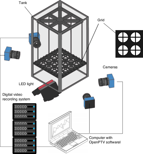
Figure 1: Schematic view of vertically oscillating grid in a glass tank. The two LED light sources provide a volumetric illumination of the flow field under the grid. Four high-speed CMOS cameras synchronously record the motion of the particles and flow tracers on a real-time video, streamed to a digital video recording system (IO Industries Inc.).

Prior to the 3D-PTV study, the flow field under the grid was characterized using particle image velocimetry (PIV), see Traugott et al. [40]. The PIV data allows to define the important scales of turbulent flow under the oscillating grid. The Kolmogorov length scales varied within the range $\eta=(\nu^{3}/\varepsilon)^{1/4}=270\div 330\>\mu\textrm{m}$ and the Kolmogorov time scales estimated as $\tau_{\eta}=\left(\eta/\nu\right)^{1/2}=0.07\div 0.1$ seconds. The flow under the grid was neither homogeneous nor isotropic as it might be expected due to the relative proximity of the grid to the bottom wall and the large solidity.

The 3D-PTV experimental system shown schematically in Fig. (1) included the following components: the digital video recording system (IO Industries Inc.) and four high speed CMOS cameras ($8\ \mathrm{bit}$, $1280\times 1024\ \mathrm{pixels}$, EoSens GE, Mikrotron), equipped with $60$ mm lenses (F-mount, Nikon). The cameras capture simultaneously (with a maximum possible time jitter of $0.001\ \mathrm{fps}$) digital video recorded at the rate up to $700\ \mathrm{M\mathrm{b/s}}$ on high-speed hard drives. The data is analyzed using the open source software, “OpenPTV” [32].

Cameras were located in an angular array from two sides of the grid chamber, as shown in Fig. (1). The four cameras arrangement reduces the number of ambiguities and allows reliable determination of most of the particles which are completely hidden in one of four images [10]. In the particular runs reported here, image acquisition rate was set to $160$ fps, the observation volume was $7.5\times 4\times 6$ cm³ (length $\times$ width $\times$ height). Two light emitting diodes (LED) line sources (Metaphase, USA) illuminated the observation volume in the center of the grid chamber. The combination of the two LED light sources provided a nearly uniform light intensity across a wider observation volume. A two step calibration method was used: a static calibration using a three-dimensional reference target, and a dynamic calibration using a dumbbell (wand) moving in a measurement volume after the grid was installed in the operating condition [32].

Two different types of particles were used in order to obtain simultaneous recordings of the turbulent flow and the motion of the inertial particles in the same observation volume. Polyamide particles with a mean diameter of $50\ \mathrm{\mu m}$ and density of $1030$ kg/m³ (Dantec Dynamics Inc.) were used as tracers. The relaxation time of flow tracers, $\tau_{p}=\rho_{p}d_{p}^{2}/18\mu$ is approximately $0.143$ ms, which is significantly smaller than the Kolmogorov time scale of the flow and their Stokes number is small, $St<0.01$. Furthermore, the particles fulfill the conservative restrictions for flows with acceleration of less than $10\ \mathrm{m/s^{2}}$ e.g. Dracos [10] (see class of neutrally buoyant, $d_{p}<60\ \mathrm{\mu m}$ particles), and therefore behave as tracers in a given turbulent flow.

Silica gel spheres (Fulka Inc.), $550$ $\mu m$ in diameter (of the order of magnitude of the Kolmogorov length scale) and effective density of $\rho_{p}=1062$ kg/m³ were used as the inertial particles. Their Stokes number is approximately equal to 0.2.

Before each experimental run, approximately 30 inertial particles were spread randomly on the bottom. Each run started in stagnant water, and after a certain time the inertial particles were entrained into the water column by the turbulent flow generated under the constantly oscillating grid. For the chosen frequencies ($1.5,1.7,1.9$ and $2.1$ Hz), all inertial particles became suspended. The number of particles spread on the bottom of the tank is relatively low and they are lifted-off separately, without particle-particle interactions. 3D-PTV analysis, including particle identification and tracking, was performed on the inertial particles separately from the tracers using the same video files. The software [32] allows to discriminate between the particles and the tracers using their size.

It is important to note that the number of “successful| events of inertial particles that participate in the statistics in different runs were only 8 $\div$ 20. These are neither the total number of the events nor the total number of trajectories recorded by 3D-PTV. The 30 particles spread on the bottom wall of a tank move freely in all possible directions. Some particles reach the corners of the tank, while a majority is freely moving in the tank going through numerous suspension - deposition cycles. Nevertheless, the number of “successful” events relate to a very small sample selected by post-processing. These events: a) occur within the field of view of the 3D-PTV system (many particles are lifted outside of the volume or start their motion inside and lift-off ends outside of the volume, etc.), b) are successfully tracked during the full length of the event (due to the restrictions of Basset force estimate we had to have the particle within the field of view for at least 10 time steps prior to upward motion), c) the particles are lifted-off and not deposited for at least 10 Kolmogorov times (otherwise the event is denoted as saltation) , d) have sufficient tracer density surrounding the particle before, during and after the lift-off event. Due to this large set of complex restrictions, the amount of “successful” events that we can add into the statistics is relatively small. Collection of more data was impossible due to the large time span of the experiment and data analysis.

2.2 Particle equation of motion

The method used herein to estimate the forces acting on the particles is described in details in Meller and Liberzon [26], and briefly reproduced here for completeness. The main difference is the estimate of the Basset force as explained below. The method is based on the equation of motion of a point-like sphere in a non-uniform flow, presented by Maxey and Riley [23] based on the previous model of Corrsin and Lumely [8]. There are five dominant terms of forces acting on a point-wise particle in Eq. (1).

$$m_{p}\frac{d\boldsymbol{u}_{p}}{dt}=m_{f}\left(\frac{D\boldsymbol{u}_{f}}{Dt}-\nu\nabla^{2}\boldsymbol{u}_{f}\right)-0.5m_{f}\frac{d}{dt}\boldsymbol{U}_{rel}-6\pi r_{p}\mu\boldsymbol{U}_{rel}-\\ -6\pi r_{p}^{2}\mu\int_{-\infty}^{t}\frac{d\boldsymbol{U}_{rel}/d\tau}{\sqrt{\pi\nu(t-\tau)}}d\tau+(m_{p}-m_{f})\boldsymbol{g}$$ (1)

here $\boldsymbol{u}_{p}$ represents particle velocity, $m_{p}$ is the mass of the particle with radius $r_{p}$ , $\boldsymbol{u}_{f}$ represents the undisturbed fluid velocity at the particle position, $m_{f}$ the mass of fluid displaced by the particle, $\boldsymbol{U}_{rel}$ represents the relative velocity between the particle and the fluid. The notation $\frac{d}{dt}=\frac{\partial}{\partial t}+\boldsymbol{u}_{p}\cdot\nabla$ indicates a full (Lagrangian) derivative following the moving particle, while $\frac{D}{Dt}=\frac{\partial}{\partial t}+\boldsymbol{u}_{f}\cdot\nabla$ represents the material derivative of the moving fluid element. The terms on the right side of Eq. (1) are the pressure gradient force $\boldsymbol{F}_{p}$, the added-mass force $\boldsymbol{F}_{a}$, the Stokes drag force $\boldsymbol{F}_{s}$, the Basset (history or viscous unsteady) force $\boldsymbol{F}_{b}$, and the buoyancy force $\boldsymbol{F}_{g}$, respectively. This equation was developed for an isolated, point-like particle in the bulk of a smooth uniform flow, far from any boundary so that particle-particle and particle-boundary interactions are excluded. There is also no lift force term for the point-like particle.

The formulation of Maxey and Riley [23] keeps the buoyancy term but replaces the added mass, Basset, and the Stokes drag terms with expressions modified by the Laplacian of the local fluid velocity field, known as “the Faxén corrections”, see for example Calzavarini et al. [5]. Although the equation of motion relies on the assumption that the particle is much smaller than the smallest scales of the flow, it was shown that also in cases when the particle is of the order of the Kolmogorov length scale, the error is not significant [2, 39]. Calzavarini et al. [4] have shown that the Faxén correction becomes significant for particles with a diameter of ten times larger than the dissipative length scales of the flow. In our experiments, the inertial particle size is of the order of the Kolmogorov length scale. Therefore we use the form of the terms that does not contain the Faxén corrections.

Sridhar and Katz [38] reported force measurements on bubbles in a laminar vortex flow based on the Maxey and Riley [23] formulation. In their study neighboring bubbles were used to estimate the local fluid velocity. The Basset force and Faxén correction were neglected, the Stokes drag was replaced with a general drag term and the additional lift force term was introduced. The procedure involved the measurement of the pressure, inertia and buoyancy forces on each bubble (based on the interpolation of velocity of the neighboring bubbles) and balancing their resultant $(\boldsymbol{F}_{T})$ with the lift and drag forces. Drag and lift forces are therefore the parallel and normal components with respect to the vector of relative velocity between the particle and the fluid, $\boldsymbol{U}_{rel}$. Recently Meller and Liberzon [26] extended the method of Sridhar and Katz [38] for the turbulent flow case by using two-phase (tracers/particles) experimental data of Guala et al. [13]. In Sridhar and Katz [38], Meller and Liberzon [26] notation, the balance of forces is:

$$\boldsymbol{F}_{T}=\boldsymbol{F}_{D}+\boldsymbol{F}_{L}=-(\boldsymbol{F}_{g}+\boldsymbol{F}_{p}+\boldsymbol{F}_{i}+\boldsymbol{F}_{b})$$ (2)

where the inertia force is defined for the sake of brevity as follows:

$$\boldsymbol{F}_{i}=m_{p}\frac{d\boldsymbol{u}_{p}}{dt}-\boldsymbol{F}_{a}$$ (3)

And the drag and the lift are defined as:

$$\boldsymbol{F}_{D}=\frac{\boldsymbol{F}_{T}\cdot\boldsymbol{U}_{rel}}{\left|\boldsymbol{U}_{rel}\right|}$$ (4)

$$\boldsymbol{F}_{L}=\boldsymbol{F}_{T}-\boldsymbol{F}_{D}$$ (5)

In the present study we use the method of Sridhar and Katz [38], Meller and Liberzon [26], applied to estimate forces on inertial particles before and during the lift-off in turbulent flows, based on the particle motion and the local flow analysis. Since we study the particle lift-off events of freely moving particles (after their incipient motion), the particle contact time with the surface is very short, therefore particle-surface forces, such as adhesion and contact, can be neglected.

The Basset “history” force accounts for the viscous unsteady effect and for the temporal delay in particle response. The delay is due to the time it takes for the boundary layer on the surface of a particle to adjust to the varying relative velocity. According to its definition in Eq. (1), this term is calculated as an integral from the the moment of incipient motion to the present time. Because turbulent flows change rapidly, the earlier moments contribute a negligible portion and the term can be approximated using only a few recent time steps. Mei and Adrian [25] examined the inertial effects on the history force and found that for finite particle Reynolds numbers, the Basset kernel behaves a $t^{-1/2}$ for short times and decays at a faster rate proportional to $t^{-2}$ at larger times. More recent studies of Bombardelli et al. [1], Lukerchenko [18], Olivieri et al. [31] demonstrated that the Basset force is important for relatively small particles moving close to solid boundaries, and should be included in Lagrangian models of bed-load transport if the particle settling velocity Reynolds number ($Re_{W}=W_{s}d_{p}/\nu$) is below 4000 (where $W_{s}$ is settling velocity, in our case it is $\approx 11$ mm/s), and the density ratio $s=\rho_{p}/\rho_{f}$ is of the order $1-10$. Ling et al. [17] have examined the unsteady force terms and have shown their importance for particles of size comparable with the Kolmogorov length scale. The authors also studied whether it is possible to simplify the history integral, and provided a useful criteria for the choice of a simplified method. Based on the Kolmogorov time scale estimate (in our case $\tau_{\eta}\approx 0.1$ s), and the viscous-unsteady time scale defined in Mei and Adrian [25], Ling et al. [17] as $\tau_{\mathrm{vu}}=\frac{d_{p}^{2}}{\nu}(\frac{4}{\pi})^{1/3}(\frac{0.75+0.105Re_{p}}{Re_{p}})^{2}$ (in our cases $0.005\div 0.07$ seconds) we verify that $\tau_{\mathrm{vu}}<\tau_{\eta}$. Therefore, we define the Basset viscous unsteady kernel in the following analysis, in the form of Eq. (1), but integrating for the short interval of $t-0.5\tau_{\eta}$.

The Reynolds number based on the local relative velocity $\boldsymbol{U}_{rel}$ between the particle and local flow ($Re_{r}=\boldsymbol{U}_{rel}d_{p}/\nu$) at the moment of lift-off was found in the range of $2\div 50$. The schematic definition of the local relative velocity is shown in Fig. (2). A solid particle (large sphere) is moving along the bottom all at velocity $\boldsymbol{u}_{p}$. Neighbor tracers ($i=1\ldots N$), move near the solid particle position, distant by distance $r_{i}$.

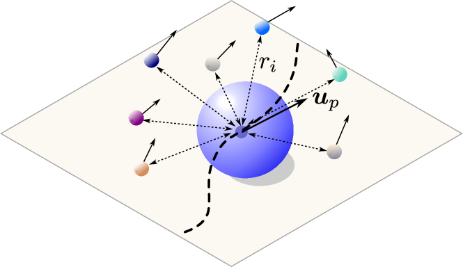
Figure 2: Scheme of definition of the relative velocity $\boldsymbol{U}_{rel}$ between the particle moving at velocity $\boldsymbol{u}_{p}$ and neighbor tracers, moving at center-to-center distance $\boldsymbol{r}_{i}$. Dashed line is a schematic trajectory of the particle.

We implement the same analysis as in Meller and Liberzon [26] of inverse distance weighting interpolation (sometimes denoted as Shepard interpolation) see Shepard [35]. The interpolated value that represents the undisturbed velocity at the position of the solid particle is:

$$\boldsymbol{\left\langle u\right\rangle}=\frac{\sum_{i}u_{i}r_{i}^{-p}}{\sum_{i}r_{i}^{-p}}$$ (6)

where $p$ is the parameter, determined empirically. In this case the vector of relative velocity is defined through the interpolated value, and the angular brackets hereinafter define quantities that are derived similarly:

$$\boldsymbol{U}_{rel}=\left\langle\boldsymbol{u}-\boldsymbol{u}_{p}\right\rangle$$ (7)

Quality of the relative velocity estimate depends on the distribution of tracers surrounding the particle, namely the number, velocity, acceleration and distance $r_{i}$. Tracer self-test is a fidelity measure applicable to our case, similarly to the method used by Cisse et al. [7] to compare the effects on tracers versus inertial particles. In our case we use the interpolation method at the positions of the tracers themselves and compare it to the measures at the position of the measured particles. In the case of tracers Meller and Liberzon [26] have suggested to use the statistical self-description index test us a group of tracers (in all measurements). We repeated this analysis to find the power exponent $p=3$ to be the optimal choice for the present case. The probability density function (PDF) of relative velocity $\boldsymbol{U}_{rel}$ for tracers and solid particles is expected to be significantly different. Such comparison is shown in Fig. (3). The results are similar to those of Sridhar and Katz [38], Meller and Liberzon [26]. It is important to note that the relative velocity magnitude of 1-2 cm/s is one to two orders of magnitude smaller than the flow velocity in this experiment and points out that our freely moving particles move along the wall with the velocity only slightly different from the flow velocity.

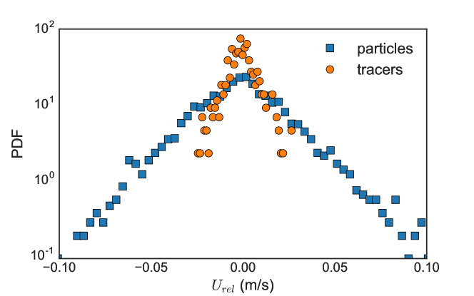
Figure 3: Probability density function of relative velocity components for solid particles (squares) and flow tracers (circles), estimated through Eq. (6).

It is important to note that our main goal is to estimate relative contribution of the force terms before, during after the lift-off events based on local turbulent flow parameters. Taking into account the inhomogeneous distribution of flow tracers near the wall, we deal with an additional trade-off in the selection of the number of nearest neighbor tracers. We first encountered this problem in our preliminary study Traugott et al. [40] and studied it in more details in Meller and Liberzon [26]. Force estimate using Lagrangian data based on Eq. (2) requires tracers to stay within the particle neighborhood for a certain time. This is especially important for the Basset force estimate. Strongly fluctuating number of tracers during the time interval of particle lift-off event adversely affects the results. We also experience an optical problem: tracers that are too close to the particle are being shaded and disappear from tracking database. Following the tracers self-test and sensitivity analysis of the inverse distance weighting parameter $p$, we found that the force estimate would not vary significantly if we include in the interpolation particles that are closer than $80\eta$ from the center of a solid particle in the horizontal direction (the diameter of the particles is of the order of the Kolmogorov length scale, $\eta$), and less than $30\eta$ in the wall-normal direction. These restrictions act in addition to the inverse distance weighting method that increases weights of the nearest neighbors and reduces weights of the tracers beyond 2-3 particle diameters. As an outcome of these restrictions, at each time step, forces were calculated based on $20\div 100$ tracers.

We also need to describe in details how the forces are estimated from the Lagrangian data. Buoyancy force is estimated based on the average particle radius $r_{p}$ and density $\rho_{p}$ according to Eq. (8) and this is the only force component that does not depend on the data:

$$F_{g}=\frac{4}{3}(\rho_{p}-\rho_{l})g\pi r_{p}^{3}$$ (8)

Buoyancy acts on the inertial particles downwards (i.e. in the negative $y$ direction) and on average, taking into account the size distribution of the solid particles, its magnitude is $5.7\times 10^{-8}$ N.

The pressure and inertia forces were calculated from the Lagrangian acceleration of the inertial particle and that the local flow surrounding it, according to Eq. (9) and  (10) respectively (see Meller and Liberzon [26] for more details):

$$\boldsymbol{F}_{p}=\frac{4}{3}\rho_{l}\pi r_{p}^{3}\left\langle\frac{D\boldsymbol{u}_{f}}{Dt}\right\rangle$$ (9)

$$\boldsymbol{F}_{i}=-\frac{4}{3}\pi r_{p}^{3}\left(\rho_{p}\frac{d\boldsymbol{u}_{p}}{dt}+m_{a}\rho_{l}\left\langle\frac{D\boldsymbol{u}_{p}}{Dt}-\frac{D\boldsymbol{u}_{f}}{Dt}\right\rangle\right)$$ (10)

where $\left\langle\frac{DU_{f}}{Dt}\right\rangle$ is the interpolated acceleration evaluated at the center of the solid particle according to Eq. (6). $\left\langle\frac{Du_{p}}{Dt}-\frac{Du_{f}}{Dt}\right\rangle$ denotes the average difference between particle and tracers accelerations. The first term in the inertia force is the body force of the particle, which depends on the mass and acceleration of the particle. The second term is the apparent mass force. According to literature, for instance Meng and Van der Geld [27], the so-called added mass coefficient of the solid particles is $m_{a}=0.5$. The Basset force was estimated according to the definition and taking into account the finite time kernel as shown by Mei and Adrian [25]:

$$\boldsymbol{F}_{b}=6\pi r_{p}^{2}\mu\intop_{t-0.5\tau_{\eta}}^{t}\frac{d\boldsymbol{U}_{rel}/d\tau}{\sqrt{\pi\nu(t-\tau)}}$$ (11)

which means that the average relative velocity was differentiated in time to obtain the relative acceleration term $d\boldsymbol{U}_{rel}/d\tau$. At each time step, the Basset force was calculated using the backward finite-difference scheme, based on the previous time steps. We have verified that the Basset force value does not change if we integrate longer than 1/2 the Kolmogorov time scale.

The force vector that balances the sum of the buoyancy, inertia, pressure and Basset force terms is called the total force, $\boldsymbol{F}_{T}$, according to Eq. (2). Following Sridhar and Katz [38], Meller and Liberzon [26], the total force vector was decomposed into two orthogonal components to obtain the magnitude of the drag and lift forces. Drag is the component of total force parallel to the relative velocity, $\boldsymbol{U}_{rel}$ and the lift is perpendicular to it, according to Eqs. (4) and  (5).

3 Results and discussion

Particle tracking velocimetry experiments provide the Lagrangian trajectories defined as locations of particles in time and space, $\boldsymbol{x}_{p}(t)$, for large particles and $\boldsymbol{x}_{f}(t)$ for flow tracers. Fig. (4)(a) presents a three-dimensional view of an example of Lagrangian trajectory exemplifying a lift-off event of a large particle as it leaves the wall and moves upwards, along with numerous trajectories of tracers surrounding the particle at different time instants. Coordinates are given in millimeters with respect to the origin predefined by the calibration target, $y$ is the vertical (parallel to gravity) direction. Fig. (4)(b) demonstrates a more quantitative analysis of the position, velocity and acceleration vector components in time of the particle. A combination of the visual and quantitative information illustrates the complexity of the problem. At the beginning, for the first two Kolmogorov time scales, the particle moves along the wall ($y=-21$ mm), as we see the values change only for $x$ and $z$ components. The particle is either sliding or rolling on the bottom wall. At approximately $2\tau_{\eta}$ the lift-off event occurred and the particle resuspended into the flow. After the lift-off event (after detachment from the wall) all the velocity and acceleration components change, as expected for a three-dimensional turbulent flow case. The plot also underlines the intrinsic difficulty to define the precise time instant of the lift-off event as the vertical position, velocity and acceleration components do not change instantly. The definition of the detachment can be based on either position, velocity or acceleration, as we discuss in the following.

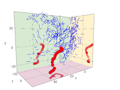
(a)

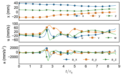
(b)

Figure 4: (a) Isometric sketch of a Lagrangian trajectory of a lifted particle. (b) Position, velocity and acceleration components of a particle experiencing the lift-off event. The frequency in this run was 1.7 Hz.

3.1 Definition of the lift-off event

We distinguish the moment of lift-off from the typically defined incipient motion, which is the beginning of particle movement on the bottom surface from a fixed position. Although we could track particles that at some moment of time have zero velocity, this experiment is difficult to perform on freely moving particles. We focus on the lift-off of the freely moving particles but we also include the events of the particles that are lifted with a negligible horizontal velocity. The moment of lift-off and the influence of the local flow characteristics and fluid-particle forces on the event and particle motion is our major focus.

A standard lift-off event is defined as the detachment of a particle from the wall, i.e. breaking the contact with the surface. Zooming into the data to visualize the event, as shown in Fig. (5), we identify the predictable scenario: first, at one Kolmogorov time scale from the arbitrary time instant defined as $t_{0}$ the acceleration component $a_{y}$ changes to positive and its value increases monotonically; after additional $1/5\tau_{\eta}$ (about $20$ milliseconds), the vertical velocity value changes (other velocity components change continuously as shown in Fig. (4)) and only after additional $1/3\tau_{\eta}$ (30 msec) the $y$ coordinate changes and the particle detaches from the wall. It means that one could define the moment of lift-off by either the first moment of the positive acceleration, positive velocity or the last moment of $y=y_{wall}$. In addition, one has to take into account the experimental uncertainty, thus the definition has to be dependent on some time or magnitude threshold.

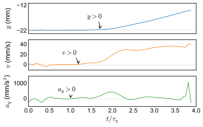
Figure 5: Vertical components of position, velocity and acceleration of a resuspended particle during the lift-off event, extracted from the run at 1.5 Hz.

Although the time interval of the lift-off event is shorter than one Kolmogorov time scale, we emphasize that the definition of the moment of the event based on one of the properties might affect the analysis and the results. The time point for lift-off in this study is defined in this study as the first time step in which the position of the particle in $y_{p}>y_{wall}+0.1$ mm, disregarding changes in position smaller than the 1/5 of the particle diameter (small jumps during the horizontal motion along the wall). In order for the event to be considered as a lift-off event, the particle must remain in suspension for at least 1/2 Kolmogorov time scale after the detected moment. If a particle returned to the bottom and remained on the wall for at least another 1/2 Kolmogorov time scale, a separate lift-off event of the same particle could be identified. As we explained in the Section (2), out of many resuspension events, only those that were within the field of view of the 3D-PTV system, successfully tracked during the full length of the event, got lifted and not land immediately afterward and have sufficient tracer density surrounding the lift-off event, were considered for the following analysis.

3.2 Forces on particles before and during lift-off events

Forces acting on the particles during lift-off events were estimated according to the methods described in Section (3.2). Fig. (6)(a) exemplifies a Lagrangian trajectory of a lifted-off particle, demonstrating the relative magnitude and direction of the forces acting on the particle, particle velocity $(\boldsymbol{u}_{p}$) and the relative velocity $(\boldsymbol{U}_{rel}$) between the particle and local fluid at each time step: before, during and after lift-off. Fig. (6)(b) demonstrates the magnitudes of the forces acting on the particle in time normalized by the magnitude of buoyancy force. The moment of lift-off is marked by the red point. We observe that the force terms, excluding drag, are of similar magnitude before the lift-off event. The drag force is much smaller as compared to other terms. The magnitude of lift, inertia and Basset forces increase about 4-10 time steps (1/4-2/3$\tau_{\eta}$) right before the lift-off and remain high until 10 time steps (2/3 $\tau_{\eta}$) after the lift-off event. As the particles are fully entrained, they move almost like the tracer particles in a strong turbulent flow and the relative velocity sharply decreases, as was estimated by Meller and Liberzon [26]. Here we focus only on the relative magnitude of the different terms of forces before and during the lift-off with an emphasis on the magnitude of Basset force. The magnitude of Basset force is approximately one-half of lift force value before the lift-off event, and shows the largest values at and after the lift-off. The magnitude of the drag force is the least important in this type of resuspension events, approximately two orders of magnitude lower than the lift force. This finding is in apparent contradiction with the large body of literature that emphasizes the drag force over lift force. It is explained by the fact that the particle is already moving (either sliding or rolling) at the velocity, which is close to that of the flow velocity in the near wall region. The lift force, as it is understood here, is caused by the local shear. The Basset unsteady-viscous force seems to be also non-negligible and contributes to the lift-off events. We also observe that $F_{T}$ is almost completely perpendicular to the relative velocity vector, such that the magnitudes of $F_{T}$ and $F_{L}$ are overlapping. Due to relatively large experimental uncertainty (as estimated in the Appendix according to standard error propagation methods) we are not able to claim the precise values of the forces acting on the particles. Nevertheless, the estimate of errors enforce that we can safely compare the magnitudes of the force components. The largest uncertainty is for the inertia force ($\varepsilon_{F_{i}}=1.2\cdot 10^{-7}\ \mathrm{N}$ ) as its value is determined by subtracting acceleration vectors. Consequently, the accuracy of drag and lift values is also limited, but it is sufficient to emphasize that the lift is at least an order of magnitude higher than the drag force.

(a)

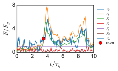
(b)

Figure 6: (a) presents an isometric sketch of a Lagrangian trajectory of a particle demonstrating the magnitude and direction of velocities and forces acting on the particle at each time step, extracted from the run at frequency of $1.7\ \mathrm{Hz}$. (b) Magnitude of the forces acting on the particle in time, moment of lift-off is marked as the red point.

One attempt to reduce the experimental uncertainty, yet preserve the insight from the measured data, is to decompose the forces differently. Instead of using a projection on the vector of relative velocity that changes abruptly in the turbulent flow near the wall, we project them on the vertical (gravity) and horizontal planes. We normalize the force components using the buoyancy force magnitude and show the horizontal and vertical components in in Fig. (7). The buoyancy force is negative in $y$ (vertical) direction and appears as a straight line in the normalized plot in Fig. (7) (a). In the horizontal direction, magnitude of all forces (except for the drag) before lift-off are similar, while in the vertical direction, magnitude of Basset and lift before lift-off are higher than pressure and inertia. The event is marked by the point in which the sum of the lift force and the Basset force is high.

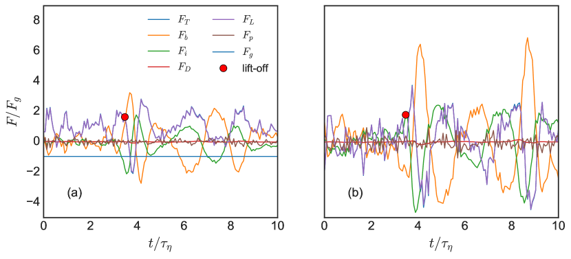
Figure 7: Time history of forces acting on the particle, obtained for the grid frequency of $1.7\ \mathrm{Hz}$, and the moment of lift-off is marked by the red point. (a) vertical components (b) horizontal components.

The inertia force equation includes two terms: the first is the body force of the particle ($-m_{p}a_{p})$, and the second is the apparent mass force. Fig. (8) presents the vertical components of body, apparent mass, pressure and Basset forces, for two different frequencies of the oscillating grid (a,b). Every line represents the ensemble averaged magnitude of the force of all the particles suspended and successfully tracked at the same frequency within the time interval of the experiment (20 and 8 particles for frequencies of $1.7$ and $1.9\ \mathrm{Hz}$ respectively). Eight time steps (1/2 $\tau_{\eta}$) before lift off, the vertical component of body force ($-m_{p}a_{p}$) decreases below zero, indicating a consistent increase of particle vertical acceleration values. This is also the time instant at which the vertical component of the body force and vertical components of apparent mass and pressure forces are separated from one another. The difference between them increases until the lift-off event. Later the vertical acceleration decreases and the difference between the forces also decrease. Since the pressure force depends only on fluid acceleration and the apparent mass force depends both on the fluid and the particle response, we interpret the situation as follows: during the lift-off event the particle moves faster than the surrounding flow in the vertical direction, moving away from the surface. As the particle moves into a faster turbulent flow in the bulk, the velocity difference between particle and flow decreases. We also note that about $0.5\div 0.7\,\tau_{\eta}$ before the lift-off, the value of the vertical Basset force component increases significantly and remains high after the lift-off event. The same trend was observed for all particles and all frequencies, shown in Fig. (8)(a-d).

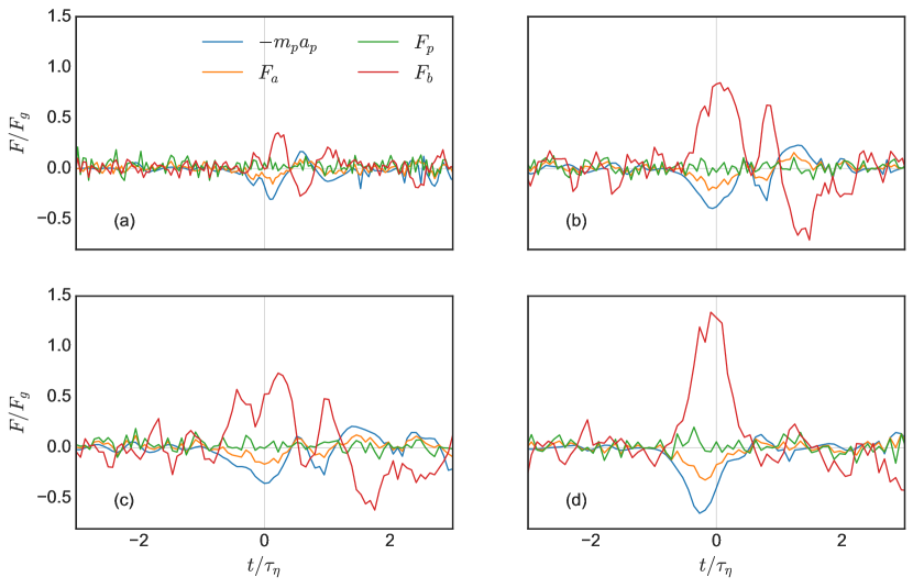
Figure 8: Vertical components of the first ($-m_{p}\boldsymbol{a}_{p}$) and second term (apparent mass force, $\boldsymbol{F}_{a}$) of the inertia force, pressure $\boldsymbol{F}_{p}$ and Basset force, $\boldsymbol{F}_{b}$ . Curves represent the ensemble averaged quantities, averaged over all trajectories at the same frequency. Panels (a-d) correspond to the frequencies 1.5 - 2.1 Hz, respectively.

We carefully examined the force traces of the particles that were lifted-off at different frequencies, different initial positions and initial velocities. We were looking for a consistent change in time that can reveal the necessary and sufficient local flow conditions that cause a lift-off event. The changes in frequencies have changed the local flow Reynolds number, and definitely changed the probability of the lift-off events. However, the local flow conditions that are responsible for the lift-off event are presumably unrelated to the global flow changes. The lift-off events we observed in our experiment are seemingly random events without any cycling or specific time scale associated with it. The only consistent and repetitive observation is of increasing Basset force (a sort of accumulative increase of relative velocity) right before the lift-off events. This observation is consistent and appears in the ensemble averaged manner for all frequencies, as shown in Fig. (8). It could imply, that the observed peaks of the Basset force are the possible triggers of the lift-off event.

4 Summary and conclusions

In the present study we obtained experimentally the fluid-related forces acting on inertial particles that are free to move on a smooth surface. We focused on the lift-off events of suspending particles into a turbulent flow without significant mean shear, unlike the wind tunnel and open water channel flow experiments. We have measured the particle trajectories along with the local flow conditions, before, during and shortly after the lift off events. In order to simplify the task of tracking fast moving particles, we worked in an oscillating grid chamber, typically used for resuspension studies. This allows to repeatedly measure the lift-off events of the same particles that are suspended and deposited, providing a large data set from which the events can be selected during the post-processing. Unique, direct simultaneous measurements of local flow conditions and 3D Lagrangian trajectories of the inertial particles, before and during lift-off, were performed using a 3D-PTV technique for several frequencies of the grid. The method of Sridhar and Katz [38] that was used to measure forces on bubbles in a laminar vortex was recently extended for the turbulent flow conditions by Meller and Liberzon [26] and used to compare the resuspension from smooth and rough surfaces by Shnapp and Liberzon [36]. Utilizing this method, the pressure, inertia and the Basset history forces were calculated from the Lagrangian acceleration of the inertial particle and the surrounding flow tracers.

We can summarize the main findings as follows. The magnitudes of all forces, excluding the drag force (which is much weaker than other terms) immediately before the lift-off event are similar. The values are close to the magnitude of the buoyancy force which we know from the particle size and density. The Basset history force (understood as a viscous unsteady force) is found to be non-negligible. Its magnitude is approximately one-half of that of the lift force before the lift-off event, and highest of all forces immediately after the lift-off event. We can conclude that this term, often neglected in numerical modeling and analysis of experimental results, has to be included in the description of the problem of resuspension of freely moving particles, especially in the liquid-solid case. Our measurements are in very good agreement with recent investigations that took a numerical approach [1, 18, 31] as they fall into the same range of parameters, i.e. $Re_{w}=W_{s}d/\nu<4000$ and $s=\rho_{p}/\rho_{f}\approx 1$.

Clearly these findings do not necessarily extrapolate to the cases of particles much heavier than the fluid. In order to understand the contribution of the Basset force to the lift-off (and possibly to the incipient motion in general), additional studies are required; for instance, different particle to fluid densities ratios, $s\gg 1$, such as gas-particle flows or addition of the mean streamwise velocity and the effect of boundary layers.

Furthermore, the distributions of forces acting on inertial particles in this type of a turbulent flow indicate that the magnitude of lift is dominant in this case. In addition, as the magnitude of the total force measured from particle acceleration $F_{T}$ and lift forces are very similar, the lift force can be estimated indirectly from much simpler experiments that do not involve two-phase tracking.

While searching for the necessary and sufficient flow conditions that precede or define the lift-off event, we have found a peculiar persistent increase of Basset force before the lift-off. This fact points to a possible trigger required for lift-off event to occur. Our results, although performed in different settings, could be in some sense related to the recent findings of Celik et al. [6], among others. The authors suggested that the time interval of the force acting on the particle is more important that its value. It is possible that our important finding of the Basset force relates to the same viscous unsteady effects that are all related to the establishment of the boundary layer and the wake of the particle. Other studies have already mentioned the importance of the pressure gradient in mobilizing particles, for instance of Schmeeckle et al. [34], Zanke [42]. We arrived to a similar conclusion observing the increase of the Basset force.

It is important to remember that we do not resolve the flow close enough to the particle in order to claim that we can accurately estimate the magnitude of the force. The experimental trade-off could lead to overestimated or underestimated values. The important part, nevertheless, is the comparative study of the force terms that are derived with a similar experimental uncertainty. In order to get a better view of the proposed mechanisms, a much higher resolution of the instantaneous flow fields and additional pressure gradient measurements below and above the test particles, before and during the moment of lift-off, are required. Such an experiment, however, seems not to be feasible in the visible future as it will require a super-resolution 3D-PTV, along with the pressure-sensitive painting or miniature pressure catheters embedded in the flow at the place and time of particle resuspension. It is possible that the accurate numerical simulations that resolve both the large and the small scales and track the solid particles in the flow, could provide a supportive evidence. We also hope that the obtained results can be helpful for the better predictions in the fields of sediment transport, pneumatic conveying, fluidized bed and bio-reactor design.

Appendix A Particle Tracking Velocimetry and uncertainty analysis

A.1 Post-processing of 3D-PTV

The main tool in our work is the three-dimensional particle velocimetry (3D-PTV), explained in details in a collection of works, for instance Mass et al. [22], Malik N.A [21], Dracos [10]. The work of Lüthi et al. [19] also provides a careful error analysis of velocity and velocity derivatives data. For the sake of clarity we briefly review here the main steps and in the following the errors and uncertainty analysis. It is noteworthy that we use the implementation of the spatial-temporal algorithm that increases the tracking efficiency and allows to work with particle seeding densities high enough to measure velocity derivatives.

3D-PTV comprises of two major steps (after the calibration part that is the main source of the bias error, described below): i) determination of particle positions in space, and ii) tracking (linking) of tracers (or particles) in consecutive images. The spatial-temporal algorithm exploits the redundant information in image (pixels) and space (mm) of several snapshots, reducing the error of particle positions in time, $x(t)$. Tracking step involves the a) search in the radius adapted using the maximum velocities, b) limited Lagrangian acceleration, c) heuristic choice of the trajectory after 4 consecutive time steps with the total minimal Lagrangian acceleration. The raw data in a form of linked positions of tracers/particles are processed using a low-pass, moving cubic polynomial filter Lüthi et al. [19], providing their filtered positions, velocities and accelerations. The filter is defined as

$$\widehat{x}(t)=c_{0}+c_{1}t+c_{2}t^{2}+c_{3}t^{3}$$ (12)

The expression is fitted to 21 points in time, from $t-10\Delta t$ to $t+10\Delta t$, for each component ($x,y,z)$ at each time step, $t$ . The filtered velocities and accelerations are defined from the polynomial coefficients:

$$\widehat{u}(t) = c_{1}+2c_{2}t+3c_{3}t^{2}$$

$$\widehat{a}(t) = 2c_{2}+6c_{3}t$$

Using filtered velocities, $\widehat{u}(x,t)$, spatial and temporal derivatives could be interpolated for every particle trajectory point. If the seeding density is sufficient, the linear approximation is

$$\widehat{u}(x_{0})=c_{0}+c_{1}x+c_{2}y+c_{3}z$$ (13)

where

$$c_{1}=\frac{\partial u}{\partial x},\quad c_{2}=\frac{\partial u}{\partial y},\quad c_{3}=\frac{\partial u}{\partial z}$$

In theory, four neighbors are sufficient to solve the equation and estimate the four coefficients, $c_{i}$. In reality, the errors in filtered velocities lead to a large error propagation. Therefore, we use over-determined linear system with information from $n>4$ points, that is solved using the least-square method:

$$\boldsymbol{A}c=u,\quad c=\left(\boldsymbol{A}^{T}u\right)\left(\boldsymbol{A}^{T}\boldsymbol{A}\right)^{-1}$$ (14)

where $\boldsymbol{A}$ is the matrix of positions. Similarly the temporal derivative is obtained, through the ansatz:

$$\widehat{u}(x_{0})=c_{0}+c_{1}x_{1}+c_{2}x_{2}+c_{3}x_{3}+c_{4}t$$ (15)

In this case, the time span for the time derivative is 4 time steps, $4\Delta t$ and the estimate is the least-squares central difference gradient method with a residual error of the order of $\mathcal{O}(\Delta t)^{2}$. We suggest the reader to refer to Lüthi et al. [19] the full description of the method and careful error analysis of a general 3D-PTV experiment and data processing that leads to the high order estimates. The tests and checks standard and embedded in our post-processing software OpenPTV consortium [32] verify that the local analysis fulfills the relative divergence $\delta\leq 0.1$, defined as

$$\delta=\frac{\left|\partial u/\partial x+\partial v/\partial y+\partial w/\partial z\right|}{\left|\partial u/\partial x\right|+\left|\partial u/\partial y\right|+\left|\partial u/\partial z\right|}$$ (16)

The errors of Lagrangian accelerations, $a=Du/Dt$ , are defined directly from the measurements along particle trajectories (see below the quantitative analysis). The components of accelerations, namely local acceleration $a_{l}=\partial u/\partial t$ and convective acceleration, $a_{c}=u_{j}\partial u_{i}/\partial x_{j}$ are estimated using the locally interpolated velocities and velocity derivatives, as described above. It is important to note that both errors are significantly larger than the one of the Lagrangian, full material derivative, yet the values of the local and convective acceleration in turbulence are also order of magnitude larger than the magnitude of Lagrangian acceleration. Nevertheless, Lüthi et al. [19] have compared the theoretical analysis with the empirical values, to show that the conservative estimate of the relative error is $\epsilon_{a_{c}}\approx 20\%$.

A.2 Uncertainty analysis of the experiment

Uncertainty analysis starts from a review of the error sources in the measurements.

The independent variable that determines the 3D-PTV accuracy is the three-dimensional (3D) particle coordinate in the laboratory frame of reference, $x,y,z$. Every particle has its own identity and its trajectory is defined by its position at each time step. Without going into details of the 3D-PTV method, there are two sources of error: a) random, precision-type errors due to the image processing algorithm that detects the center of a particle in multiple camera views, and b) systematic error due to 3D calibration of the imaging system.

The standard image processing routines provide precision of $0.05\ \mathrm{pixel}$ for the particle centroid. However for realistic images of imperfectly spherical particles and illumination non-uniformity we estimate the positioning error of $0.2\ \mathrm{pixel}$ Dracos [10].

Calibration errors arise from several sources: residual lens aberrations, imprecision in calibration target production and incorrect positioning of the calibration target. Stationary calibration process uses a high-precision machined calibration target with numerous target points outnumbering the number of equations of the photogrammetric model. The software iteratively solves the error minimization problem of the over-determined system and estimates the camera interior and exterior parameters. During the calibration process, the differences between the known points on the calibration target and the computed points are estimated. In the presented experiment, the errors in the calibration were estimated as $\varepsilon_{x}=\varepsilon_{y}=\pm 10\ \mathrm{\mu m}$ in the direction parallel to the imaging plane and $\varepsilon_{z}=\pm 30\ \mathrm{\mu m}$ in the direction parallel to the imaging axis (the magnification ratio in this experiment was $16\ \mathrm{pixel/mm}$). In order to improve the calibration error, especially in the out-of-plane direction, we have performed two additional steps: i) configuration of the cameras from both sides of the tank improves the error due to the intersection of imaging axis of the cameras from two sides (positive and negative $z$ values; ii) additional, dynamic calibration of the system using the dumbbell (wand) method OpenPTV consortium [32]. We estimate the overall positioning error to be of the order of $\epsilon_{x}=\pm 20\mu\mathrm{m}$.

Particle velocity is derived along the particle trajectory using finite difference of the particle positions in time, for instance one component is $u=\Delta x/\Delta t$. Particle tracking is performed with the high frame rate sampling (about 5-10 time steps per Kolmogorov time scale). The high time sampling allows to filter the positioning random errors (noise) using the low-pass filter Lüthi et al. [19]. Thus velocity and acceleration signals are derived as first and second derivatives of the filtered trajectories. Considering that the velocity and acceleration of the particles changes at time steps equivalent to Kolmogorov time scale of the measurements ($\tau_{\eta}=0.07-0.1\ \mathrm{s}$), the time interval for filtered velocity and acceleration error calculations can be estimated as $\triangle t=\frac{\tau_{\eta}}{5}=\frac{0.07\ \mathrm{s}}{5}=0.014\ \mathrm{s}$. The time delay is controlled by a synchronization unit with very high precision, therefore has negligible effect on the overall accuracy. Therefore velocity and acceleration errors were estimated as:

$$\varepsilon_{u}=\sqrt{2\left(\frac{\varepsilon_{x}}{\triangle t}\right)^{2}}\approx 2\ \mathrm{mm/s}$$ (17)

$$\varepsilon_{a}=\sqrt{2\left(\frac{\varepsilon_{u}}{\triangle t}\right){}^{2}}\approx 200\ \mathrm{mm/s^{2}}$$ (18)

Using the uncertainty propagation from the vector components to the vector magnitude, we obtain the following error estimates for the flow tracers (denoted with a subscript _f ) and particles (_p), velocity and acceleration.

$\left|u_{f}\right|$	$\varepsilon_{\left|u_{f}\right|}$	$\left|u_{p}\right|$	$\varepsilon_{\left|u_{p}\right|}$
0.11	0.002	0.1	0.002

$\left|a_{f}\right|$	$\varepsilon_{\left|a_{f}\right|}$	$\left|a_{p}\right|$	$\varepsilon_{\left|a_{p}\right|}$
7.0	0.2	2.1	0.2

Table 1: Estimated flow (tracers) and particles velocity and acceleration errors, (m/s, m/s²).

A.3.1 Force estimates uncertainty analysis

The buoyancy force depends only on the measurements of the particle density, $\rho_{p}$, fluid density $\rho_{f}$ and the particle radius $r_{p}$,

$$F_{g}=\frac{4}{3}(\rho_{p}-\rho_{f})g\pi r_{p}^{3}$$ (19)

The error depends on $\rho_{p}$ and $r_{p}$ and can be evaluate as follow:

$$\varepsilon_{F_{g}}=\sqrt{\left(\frac{\partial F_{g}}{\partial\rho_{p}}\varepsilon_{\rho_{p}}\right)^{2}+\left(\frac{\partial F_{g}}{\partial r_{p}}\varepsilon_{r_{p}}\right)^{2}}$$ (20)

Estimated buoyancy force amplitude is $5.7\times 10^{-8}$ N, the error value is $=2.6\times 10^{-9}$ N, therefore the relative error is 4.5%.

The pressure force is estimated using the fluid material derivative along particle trajectory

$$F_{p}=\frac{4}{3}\rho_{f}\pi r_{p}^{3}\left\langle\frac{Du_{f}}{Dt}\right\rangle$$ (21)

where $\left\langle\frac{Du_{f}}{Dt}\right\rangle$ is the volume average of the Lagrangian acceleration of neighbor tracers. The region that defines the neighborhood is not well defined. It is a compromise between the sufficiently high number of tracers used for statistics and the sufficiently small radius of averaging. In any case the concept of coarse-grained fluid flow information is used, following Lüthi et al. [20], among others. In this approach the coarse-grained quantities are defined as volume integrals:

$$\langle u\rangle=\frac{1}{\forall}\int_{\forall}u(x+x^{\prime})d^{3}x^{\prime}$$ (22)

Lüthi et al. [20] have shown the convergence of the statistics of the coarse-grained quantities that depends mainly on the seeding density of the tracers. The minimum number of particles was found to be 12 $\div$ 15 in order to achieve a convergent statistics. The test is the value of the coarse-grained (or volume averaged) quantity of interest at monotonically increasing volume of averaging volume, $\forall$. In our experiment the size of the volume corresponds to a sphere of $25\ \mathrm{mm}$. The error in the mean Lagrangian acceleration of tracers was estimated by the standard deviation of tracers acceleration and the number of tracers. The number of tracers was chosen as the lowest number of tracers observed at a specific time step in order to obtain the highest possible error; $\varepsilon_{\langle a_{f}\rangle}=200\ \mathrm{\mathrm{mm/}s^{2}}$, $\langle a_{f}\rangle=7000\ \mathrm{m\mathrm{m/s^{2}}}$. Therefore, the estimated error of pressure force is:

$$\varepsilon_{F_{p}}=\sqrt{\left(\frac{\partial F_{p}}{\partial r_{p}}\varepsilon_{r_{p}}\right)^{2}+\left(\frac{\partial F_{p}}{\partial\overline{a_{f}}}\varepsilon_{\left\langle a_{f}\right\rangle}\right)^{2}}$$ (23)

and the value is $\approx 1.7\times 10^{-8}$ N.

A.3.1.1 Inertia force

The inertia force is defined as:

$$F_{i}=-\frac{4}{3}\pi r_{p}^{3}\left(\rho_{p}\frac{du_{p}}{dt}+m_{a}\rho_{l}\left\langle\frac{Du_{p}}{dt}-\frac{Du_{f}}{Dt}\right\rangle\right)$$ (24)

The estimated error is:

$$\varepsilon_{F_{i}}=\sqrt{\left(\frac{\partial F_{i}}{\partial r_{p}}\varepsilon_{r_{p}}\right)^{2}+\left(\frac{\partial F_{i}}{\partial\rho_{p}}\varepsilon_{\rho_{p}}\right)^{2}+\left(\frac{\partial F_{i}}{\partial\left\langle a_{p}-a_{f}\right\rangle}\varepsilon_{\langle a_{p}-a_{f}\rangle}\right)^{2}+\left(\frac{\partial F_{i}}{\partial a_{p}}\varepsilon_{a_{p}}\right)^{2}}$$ (25)

The value we obtain $\varepsilon_{F_{i}}\approx 1.8\times 10^{-8}$ N.

A.3.1.1 Basset force

The Basset force is defined as:

$$F_{b}=6\pi r_{p}^{2}\mu\intop_{0}^{t}\frac{d\boldsymbol{U}_{rel}/d\tau}{\sqrt{\pi\nu(t-\tau)}}d\tau$$ (26)

The estimated error should be calculated as follow:

$$\varepsilon_{F_{b}}=\sqrt{\left(12\pi r_{p}\mu\int\limits_{0}^{t}\frac{d\boldsymbol{U}_{rel}/d\tau}{\sqrt{\pi\nu(t-\tau)}}d\tau\varepsilon_{r_{p}}\right)^{2}+\left(\frac{6\pi r_{p}^{2}\mu}{\sqrt{\pi\nu(t-\tau)}}\frac{\Delta\boldsymbol{U}_{rel}}{\Delta\tau}\varepsilon_{\frac{d\boldsymbol{U}_{rel}}{d\tau}}\right)^{2}}$$ (27)

The first term is of the order of $10^{-11}\ \mathrm{N}$ , at the second term , $\left(\frac{6\pi r_{p}^{2}\mu}{\sqrt{\pi\nu(t-\tau)}}\frac{\Delta\boldsymbol{U}_{rel}}{\Delta\tau}\right)$ is of the order of $10^{-5}$ N. The value of $\left(\varepsilon_{\frac{\Delta\boldsymbol{U}_{rel}}{\Delta\tau}}\right)$ should be estimated by calculating the standard deviation of the term. However, since the Basset force was calculated based on the previous 6 time steps and not every tracer appeared at each time step in the trajectory of the particles, the resulting Basset force from the effect of each tracer could not be calculated (only the relative velocity between particle velocity and the average velocity of local tracers could be calculated). Still, it can be assumed that the value of $\left(\varepsilon_{\frac{\Delta\boldsymbol{U}_{rel}}{\Delta\tau}}\right)$ is smaller than $10^{-3}$ N. Therefore, a conservative estimation for the Basset force error can be of the order of $\sim 10^{-8}$ N. .

References

- Bombardelli et al. [2008] F. A. Bombardelli, A. E. González, and Y. I. Niño. Computation of the particle Basset force with a fractional-derivative approach. Journal of Hydraulic Engineering, 134(10), 2008.
- Bourgoin and Haitao [2014] M. Bourgoin and X. Haitao. Focus on dynamic of particles in turbulence. New Journal of Physics, 16, 2014.
- Brennen [2005] C.E. Brennen. Fundamentals of Multiphase Flow. Cambridge University Press, 2005.
- Calzavarini et al. [2012] E. Calzavarini, R. Volk, E. Leveque, J. F. Pinton, and F. Toschi. Impact of trailing wake drag on the statistical properties and dynamic of finite-sized particle in turbulence . Physics: Nonlinear phenomena. Special issue on small scale turbulence, 241, 2012.
- Calzavarini et al. [2009] E. Calzavarini, R. Volk, M. Bourgoin, E. Leveque, J.-F. Pinton, and F. Toschi. Acceleration statistics of finite-sized particles in turbulent flow: the role of Faxen forces. Journal of Fluid Mechanics, 630:179–189, 2009.
- Celik et al. [2010] A.O. Celik, P. Diplas, C. L. Dancey, and M. Valyrakis. Impulse and particle dislodgement under turbulent flow conditions. Physics of Fluids, 22(4), 2010.
- Cisse et al. [2013] M. Cisse, H. Homann, and J. Bec. Slipping motion of large neutrally buoyant particles in turbulence. Journal of Fluid Mechanics, 735, 11 2013.
- Corrsin and Lumely [1956] S. Corrsin and J. Lumely. On the equation of motion for a particle in turbulent fluid . Applied Scientific Recearch, 6, 1956.
- Dixon [2006] Anne Marie Dixon. Environmental monitoring for cleanrooms and controlled environments. CRC Press, 2006.
- Dracos [1996] T. H. Dracos. Three-Dimensional Velocity and Vorticity Measuring and Image Analysis Technique: Lecture Notes from the short course held in Zurich, Switzerland. Kluwer Academic Publisher, 1996.
- Dwivedi et al. [2011] A. Dwivedi, W.B. Melville, A.Y. Shamseldin, and T.K Guha. Analysis of hydrodynamic lift on a bed sediment transport. Journal of geophisical research, 116, 2011.
- Gimenez-Curto and Corniero [2009] L.A. Gimenez-Curto and M.A. Corniero. Entrainment threshold of cohesionless sediment grains under steady flow of air and water. Sedimentology, 56, 2009.
- Guala et al. [2008] M. Guala, A. Liberzon, K. Hoyer, A. Tsinober, and W. Kinzelbach. Experimental study on clustering of large particles in homogeneous turbulent flow. Journal of Turbulence, 9(34):1–20, 2008.
- Hall [1988] D Hall. Measurements of the mean force on a particle near a boundary in turbulent flow. Journal of Fluid Mechanics, 187:451–466, 1988.
- Henry and Minier [2014] C. Henry and J.-P. Minier. Progress in particle resuspension from rough surfaces by turbulent flows. Progress in Energy and Combustion Science, 45:1–53, 2014.
- Huang et al. [2008] Y. H. Huang, J. E. Saiers, J. W. Harvey, G. B. Noe, and S. Mylon. Advection, dispersion, and filtration of fine particles within emergent vegetation of the florida everglades. Water Resources Research, 44:W04408, 2008.
- Ling et al. [2013] Y. Ling, M. Parmer, and S. Balachandar. A scaling analysis added-mass and history forces and thier coupling in dispersed multiphase flows. International Journal of Multiphase Flow , 57:102–114, 2013.
- Lukerchenko [2010] N. Lukerchenko. Basset history force for the bed load sediment transport. In IAHR European Division Congress, 2010.
- Lüthi et al. [2005] B. Lüthi, A. Tsinober, and W. Kinzelbach. Lagrangian measurement of vorticity dynamics in turbulent flow. Journal of Fluid Mechanics, 528:87–118, 2005.
- Lüthi et al. [2007] Beat Lüthi, Jacob Berg, Søren Ott, and Jakob Mann. Lagrangian multi-particle statistics. Journal of Turbulence, 8(45):1–17, 2007. doi: 10.1080/14685240701522927.
- Malik N.A [1993] Papantoniou D.A Malik N.A, Darcos TH. Particle tracking velocimetry in three dimensional flows, part 2: Particle tracking. Experiment in Fluids, 15:279–294, 1993.
- Mass et al. [1993] H.G. Mass, A. Gruen, and D.A. Papantoniou. Particle tracking velocimetry in three dimensional flows, part 1. Experiments in Fluids, 1993.
- Maxey and Riley [1983] M. R. Maxey and J. J. Riley. Equation of motion for a small rigid sphere in a nonuniform flow. Physics of Fluids, 26:883–889, 1983.
- McLean [1994] S.R. McLean. Turbulent structure over two dimentional bed forms:Implication for sediment transport . Journal of Geophysical Research: Oceans, 99(C6), 1994.
- Mei and Adrian [1992] R. Mei and R.J. Adrian. Flow past a sphere with an oscillation in the free-stream velocity and unsteady drag at finite reynolds number. Journal of Fluid Mechanics, 237:323–341, 1992.
- Meller and Liberzon [2015] Y. Meller and A. Liberzon. Particle - fluid interaction forces as the source of acceleration pdf invariance in particle size. International Journal of Multiphase Flow , 76:22–31, 2015.
- Meng and Van der Geld [1991] H. Meng and C.W.M Van der Geld. Particle trajectory computations in steady non-uniform liquid flows. ASME Fluids Engineering Division, 118:183–193, 1991.
- Middletich [1981] BS Middletich. Environmental effects of offshore oil production. Technical report, Plenum, New York, NY, 1981.
- Mollinger and Nieuwstadt [1996] A.M. Mollinger and F.T.M. Nieuwstadt. Measurement of the lift force on a particle fixed to the wall in the viscous sublayer of a fully developed turbulent boundary layer. Journal of Fluid Mechanics, 316:285–306, 1996.
- Nelson et al. [1995] J.M Nelson, R.C. Sherve, S.R. Mclean, and T.G Drake. Role of near bed turbulence structure in bed load transport and bed form mechanics. Water resourches research, 31 , Issue 8, 1995.
- Olivieri et al. [2014] S. Olivieri, F. Picano, G. Sardina, D. Ludicone, and L. Brandt. The effect of the Basset history force on particle clustering in Homogeneous and Isotropic Turbulence. Physics of Fluids , 26(4), 2014.
- OpenPTV consortium [2013] OpenPTV consortium. Open source particle tracking velocimetry. http://www.openptv.net/, 2013.
- Sarma et al. [1992] M.M. Sarma, H. Chamoun, D.S.H. Sita Rama Sarma, and R.S. Schechter. Factors controlling the hydrodynamic detachment of particles from surfaces. Colloid Interface Science, 149, 1992.
- Schmeeckle et al. [2007] M.W. Schmeeckle, J.M. Nelson, and R.L. Shreve. Forces on stationary particles in near bed turbulent flows. Journal of geophysical research, 112, 2007.
- Shepard [1968] D. Shepard. A two-dimensional interpolation function for irregularly-spaced data. In Proc. 1968 23rd ACM National Conference, pages 517–524, 1968.
- Shnapp and Liberzon [2015] R. Shnapp and A. Liberzon. A comparative study and a mechanistic picture of resuspension of large particles from rough and smooth surfaces in vortex-like fluid flows. Chem. Eng. Sci., 131:129–137, 2015.
- Soepyan et al. [2016] F. B. Soepyan, S. Cremaschi, B. S. McLaury, C. Sarica, H. J. Subramani, G. E. Kouba, and H. Gao. Threshold velocity to initiate particle motion in horizontal and near-horizontal conduits. Powder Technology, 292:272–289, 2016.
- Sridhar and Katz [1995] G. Sridhar and J. Katz. Drag and lift forces on microscopic bubbles entrained by a vortex. Physics of Fluids, 7:389–399, 1995.
- Toschi and Bodenschatz [2009] F Toschi and E Bodenschatz. Lagrangian properties of particles in turbulence. Annual Review of Fluid Mechanics, 41:379–404, 2009.
- Traugott et al. [2011] H. Traugott, T. Hayse, and A. Liberzon. Resuspension of particles in an oscillating grid turbulent flow using PIV and 3D-PTV. Journal of Physics: Conference Series, 318, 2011.
- van Rijn [1984] L.C. van Rijn. Sediment transport, Part 1: Bed load transport . Journal of Hydraulic Engineering, 110 , No. 10, 1984.
- Zanke [2003] U.C.E Zanke. On the begining of suspension from bed. Advances in Hydro-Science and Engineering, VI, 2003.
- Ziskind [2006] G. Ziskind. Particle resuspension from surfaces: Revisited and re-evaluated. Reviews in Chemical Engineering, 22(1-2):1–123, 2006.