A new $L^{p}$-Antieigenvalue Condition for
Ornstein-Uhlenbeck Operators

Denny Otten
                                     Department of Mathematics
                                     Bielefeld University
                                     33501 Bielefeld
                                     Germany

Date: March 8, 2024

Abstract. In this paper we study perturbed Ornstein-Uhlenbeck operators

$$\left[\mathcal{L}_{\infty}v\right](x)=A\triangle v(x)+\left\langle Sx,\nabla v(x)\right\rangle-Bv(x),\,x\in\mathbb{R}^{d},\,d\geqslant 2,$$

for simultaneously diagonalizable matrices $A,B\in\mathbb{C}^{N,N}$. The unbounded drift term is defined by a skew-symmetric matrix $S\in\mathbb{R}^{d,d}$. Differential operators of this form appear when investigating rotating waves in time-dependent reaction diffusion systems. As shown in a companion paper, one key assumption to prove resolvent estimates of $\mathcal{L}_{\infty}$ in $L^{p}(\mathbb{R}^{d},\mathbb{C}^{N})$, $1<p<\infty$, is the following $L^{p}$-dissipativity condition

$$|z|^{2}\mathrm{Re}\,\left\langle w,Aw\right\rangle+(p-2)\mathrm{Re}\,\left\langle w,z\right\rangle\mathrm{Re}\,\left\langle z,Aw\right\rangle\geqslant\gamma_{A}|z|^{2}|w|^{2}\;\forall\,z,w\in\mathbb{C}^{N}$$

for some $\gamma_{A}>0$. We prove that the $L^{p}$-dissipativity condition is equivalent to a new $L^{p}$-antieigenvalue condition

$$A\text{ invertible}\quad\text{and}\quad\mu_{1}(A)>\frac{|p-2|}{p},\,1<p<\infty,\,\mu_{1}(A)\text{ first antieigenvalue of $A$,}$$

which is a lower $p$-dependent bound of the first antieigenvalue of the diffusion matrix $A$. This relation provides a complete algebraic characterization and a geometric meaning of $L^{p}$-dissipativity for complex-valued Ornstein-Uhlenbeck operators in terms of the antieigenvalues of $A$. The proof is based on the method of Lagrange multipliers. We also discuss several special cases in which the first antieigenvalue can be given explicitly.

Key words. Complex-valued Ornstein-Uhlenbeck operator, $L^{p}$-dissipativity, $L^{p}$-antieigenvalue condition, applications to rotating waves.

AMS subject classification. 35J47 (47B44, 47D06, 35A02, 47A10).

1. Introduction

In this paper we study $L^{p}$-dissipativity of differential operators of the form

$$\left[\mathcal{L}_{\infty}v\right](x):=A\triangle v(x)+\left\langle Sx,\nabla v(x)\right\rangle-Bv(x),\,x\in\mathbb{R}^{d},\,d\geqslant 2,$$

for simultaneously diagonalizable matrices $A,B\in\mathbb{C}^{N,N}$ with $\mathrm{Re}\,\sigma(A)>0$ and a skew-symmetric matrix $S\in\mathbb{R}^{d,d}$.

Introducing the complex Ornstein-Uhlenbeck operator, [29],

$$\left[\mathcal{L}_{0}v\right](x):=A\triangle v(x)+\left\langle Sx,\nabla v(x)\right\rangle,\,x\in\mathbb{R}^{d},$$

with diffusion term and drift term given by

$$A\triangle v(x):=A\sum_{i=1}^{d}\frac{\partial^{2}}{\partial x_{i}^{2}}v(x)\quad\text{and}\quad\left\langle Sx,\nabla v(x)\right\rangle:=\sum_{i=1}^{d}(Sx)_{i}\frac{\partial}{\partial x_{i}}v(x),$$

we observe that the operator $\mathcal{L}_{\infty}=\mathcal{L}_{0}-B$ is a constant coefficient perturbation of $\mathcal{L}_{0}$. Our interest is in skew-symmetric matrices $S=-S^{T}$, in which case the drift term is rotational containing angular derivatives

$$\left\langle Sx,\nabla v(x)\right\rangle=\sum_{i=1}^{d-1}\sum_{j=i+1}^{d}S_{ij}\left(x_{j}\frac{\partial}{\partial x_{i}}-x_{i}\frac{\partial}{\partial x_{j}}\right)v(x).$$

Such differential operators arise when investigating exponential decay of rotating waves in reaction diffusion systems, see [1, 19]. The operator $\mathcal{L}_{\infty}$ appears as a far-field linearization at the solution of the nonlinear problem $\mathcal{L}_{0}v=f(v)$. The results of this paper are crucial for dealing with the nonlinear case, see [19].

An essential ingredient to treat the nonlinear case is to prove $L^{p}$-resolvent estimates for $\mathcal{L}_{\infty}$, [21, Theorem 4.4]. Such estimates are used to solve the identification problem for $\mathcal{L}_{\infty}$, [21, Theorem 5.1]. One key assumption to prove resolvent estimates of $\mathcal{L}_{\infty}$ in $L^{p}(\mathbb{R}^{d},\mathbb{C}^{N})$, $1<p<\infty$, is the following $L^{p}$-dissipativity condition

$$|z|^{2}\mathrm{Re}\,\left\langle w,Aw\right\rangle+(p-2)\mathrm{Re}\,\left\langle w,z\right\rangle\mathrm{Re}\,\left\langle z,Aw\right\rangle\geqslant\gamma_{A}|z|^{2}|w|^{2}\;\forall\,z,w\in\mathbb{C}^{N}$$

for some $\gamma_{A}>0$. In general, it is not easy to characterize the class of matrices $A$ which satisfy this algebraic condition. Only in a few special cases, e.g. in the scalar case $N=1$ or for general $N$ and $p=2$, one can check the validity directly.

The aim of this paper is to prove that the $L^{p}$-dissipativity condition is equivalent to a new $L^{p}$-antieigenvalue condition, namely

$$A\text{ invertible}\quad\text{and}\quad\mu_{1}(A)>\frac{|p-2|}{p},\,1<p<\infty,\,\mu_{1}(A)\text{ first antieigenvalue of $A$,}$$

which is a lower $p$-dependent bound of the first antieigenvalue of the diffusion matrix $A$. This criterion implies an upper $p$-dependent bound for the maximal (real) angle of $A$

$$\Phi_{\mathbb{R}}(A):=\cos^{-1}\left(\mu_{1}(A)\right)<\cos^{-1}\left(\frac{|p-2|}{p}\right)\in]0,\frac{\pi}{2}],\quad 1<p<\infty.$$

The relation between the $L^{p}$-dissipativity and the $L^{p}$-antieigenvalue condition seems to be new in the literature and is proved in Theorem 3.1. It provides a complete algebraic characterization and a nice geometric meaning of $L^{p}$-dissipativity for complex-valued Ornstein-Uhlenbeck operators in terms of the antieigenvalues of $A$. The proof is based on the method of Lagrange multipliers and requires to destinguish between the cases $A\in\mathbb{R}^{N,N}$ and $A\in\mathbb{C}^{N,N}$. We also discuss several special cases in which the first antieigenvalue can be given explicitly.

$L^{p}$-dissipativity of second order differential operators in the scalar but more general case has been analyzed by Cialdea and Maz’ya in [3, 5, 2, 4]. General theory of antieigenvalues has been developed by Gustafson in [7, 9] and independently by Kreĭn in [17]. Explicit representations of antieigenvalues have been established for Hermitian positive definite operators by Mirman in [18] and by Horn and Johnson in [16], and for (strictly) accretive normal operators by Seddighin and Gustafson in [28, 26, 14, 13], by Davis in [6] and by Mirman in [18]. Approximation results and the computation of antieigenvalues have been analyzed by Seddighin in [27] and [25, 24], respectively. For general theory of antieigenvalues and its application to operator theory, numerical analysis, wavelets, statistics, quantum mechanics, finance and optimization we refer to the book by Gustafson, [12]. Further applications are treated in [7, 8, 15, 11]. There are some extensions of the antieigenvalue theory to higher antieigenvalues, see [14, 28], to joint antieigenvalues, see [26], to symmetric antieigenvalues, see [22], and to $\theta$-antieigenvalues, see [23]. Historical background material can be found in [12, 10]. The method of Lagrange multipliers, that is necessary to prove our main result, is also used in [13]. The $L^{p}$-dissipativity condition can be found in [19, 21] and is used to prove resolvent estimates for complex Ornstein-Uhlenbeck systems.

The results from Section 3 and 4 are directly based on the PhD thesis [19].

2. Assumptions and outline of results

Consider the differential operator

$$\left[\mathcal{L}_{\infty}v\right](x):=A\triangle v(x)+\left\langle Sx,\nabla v(x)\right\rangle-Bv(x),\,x\in\mathbb{R}^{d},\,d\geqslant 2,$$

for some matrices $A,B\in\mathbb{C}^{N,N}$ and $S\in\mathbb{R}^{d,d}$.

The following conditions will be needed in this paper and relations among them will be discussed below.

Assumption 2.1.

Let $A,B\in\mathbb{K}^{N,N}$ with $\mathbb{K}\in\{\mathbb{R},\mathbb{C}\}$ and $S\in\mathbb{R}^{d,d}$ be such that

(A1) $$\text{$A$ and $B$ are simultaneously diagonalizable (over $\mathbb{C}$)},$$

(A2) $$\mathrm{Re}\,\sigma(A)>0,$$

(A3) There exists some $$\beta_{A}>0$$ such that

$$\quad\mathrm{Re}\,\left\langle w,Aw\right\rangle\geqslant\beta_{A}\;\forall\,w\in\mathbb{K}^{N},\,|w|=1,$$

(A4) There exists some $$\gamma_{A}>0$$ such that

$$\quad|z|^{2}\mathrm{Re}\,\left\langle w,Aw\right\rangle+(p-2)\mathrm{Re}\,\left\langle w,z\right\rangle\mathrm{Re}\,\left\langle z,Aw\right\rangle\geqslant\gamma_{A}|z|^{2}|w|^{2}\;\forall\,z,w\in\mathbb{K}^{N}$$

for some $$1<p<\infty$$,

(A5) Case ($$N=1 \mathbb{K}=\mathbb{R}$$, ):

$$\quad A=a>0,$$

Cases ($$N\geqslant 2 \mathbb{K}=\mathbb{R} N\geqslant 1 \mathbb{K}=\mathbb{C}$$, ) and (, ):

$$\quad A\text{ invertible}\quad\text{and}\quad\mu_{1}(A)>\frac{|p-2|}{p}\text{ for some $1<p<\infty$,}$$

(A6) $$\text{$S$ is skew-symmetric}.$$

Assumption (A1) is a system condition and ensures that some results for scalar equations can be extended to system cases. This condition was used in [19, 20] to derive an explicit formula for the heat kernel of $\mathcal{L}_{\infty}$. It is motivated by the fact that a transformation of a scalar complex-valued equation into a $2$-dimensional real-valued system always implies two (real) matrices $A$ and $B$ that are simultaneously diagonalizable (over $\mathbb{C}$). The positivity condition (A2) guarantees that the diffusion part $A\triangle$ is an elliptic operator. It requires that all eigenvalues $\lambda$ of $A$ are contained in the open right half-plane $\mathbb{C}_{+}:=\{\lambda\in\mathbb{C}\mid\mathrm{Re}\,\lambda>0\}$, where $\sigma(A)$ denotes the spectrum of $A$. Condition (A2) guarantees that $A^{-1}$ exists and states that $-A$ is a stable matrix. To discuss the strict accretivity condition (A3), we recall the following definition, from [7, 12].

Definition 2.2.

Let $A\in\mathbb{K}^{N,N}$ with $\mathbb{K}\in\{\mathbb{R},\mathbb{C}\}$ and $N\in\mathbb{N}$, then $A$ is called accretive (or strictly accretive), if

$$\underset{\begin{subarray}{c}w\in\mathbb{K}^{N}\\ |w|=1\end{subarray}}{\inf}\mathrm{Re}\,\left\langle w,Aw\right\rangle\geqslant 0\quad(\text{or}\quad\underset{\begin{subarray}{c}w\in\mathbb{K}^{N}\\ |w|=1\end{subarray}}{\inf}\mathrm{Re}\,\left\langle w,Aw\right\rangle>0),$$

and dissipative (or strictly dissipative), if

$$\underset{\begin{subarray}{c}w\in\mathbb{K}^{N}\\ |w|=1\end{subarray}}{\sup}\mathrm{Re}\,\left\langle w,Aw\right\rangle\leqslant 0\quad(\text{or}\quad\underset{\begin{subarray}{c}w\in\mathbb{K}^{N}\\ |w|=1\end{subarray}}{\sup}\mathrm{Re}\,\left\langle w,Aw\right\rangle<0).$$

For Hermitian matrices $A$, replace accretive (strictly accretive, dissipative and strictly dissipative) by positive semi-definite (positive definite, negative semi-definite and negative definite).

Condition (A3) states that the matrix $A$ is strictly accretive, which is more restrictive than (A2). In (A3), $\left\langle u,v\right\rangle:=\overline{u}^{T}v$ denotes the standard inner product on $\mathbb{K}^{N}$. Note that condition (A2) is satisfied if and only if

$$\exists\,\left[\cdot,\cdot\right]\text{ inner product on $\mathbb{K}^{N}$}:\quad\mathrm{Re}\,\left[w,Aw\right]\geqslant\beta_{A}>0\;\forall\,w\in\mathbb{K}^{N},\,\left[w,w\right]=1,$$

but it does not imply $\left[\cdot,\cdot\right]=\left\langle\cdot,\cdot\right\rangle$. Condition (A3) ensures that the differential operator $\mathcal{L}_{\infty}$ is closed on its (local) domain $\mathcal{D}^{p}_{\mathrm{loc}}(\mathcal{L}_{0})$. The $L^{p}$-dissipativity condition (A4) seems to be new in the literature and is used to prove $L^{p}$-resolvent estimates for $\mathcal{L}_{\infty}$ in [19, 21]. Condition (A4) is more restrictive than (A3) and imposes additional requirements on the spectrum of $A$. $L^{p}$-dissipativity results for scalar differential operators of the form

$$\mathcal{L}v=\nabla^{T}\left(Q\nabla v\right)+b^{T}\nabla v+av,\,x\in\Omega$$

has been established in [4] for constant coefficients $Q\in\mathbb{C}^{d,d}$, $b\in\mathbb{C}^{d}$, $a\in\mathbb{C}$ with $\Omega\subseteq\mathbb{R}^{d}$ open, and for variable coefficients $Q_{ij},b_{j}\in C^{1}(\overline{\Omega},\mathbb{C})$, $a\in C^{0}(\overline{\Omega},\mathbb{C})$, $i,j=1,\ldots d$, with $\Omega\subset\mathbb{R}^{d}$ bounded. In the scalar complex case with $A=\alpha\in\mathbb{C}$ and $B=\delta\in\mathbb{C}$, the choice

$$Q=\alpha I_{d},\;b=Sx,\;a=\delta,\;\Omega=\mathbb{R}^{d}$$

implies $\mathcal{L}_{\infty}=\mathcal{L}$ and leads to a differential operator with variable coefficients but on an unbounded domain. Thus, the $L^{p}$-dissipativity of $\mathcal{L}_{\infty}$ has not been treated in [4], neither for the system nor for the scalar case. Therefore, the $L^{p}$-dissipativity condition (A4), which has been established in [19, 21], can not be deduced from [4]. Recall the following definition from [7, 12].

Definition 2.3.

Let $A\in\mathbb{K}^{N,N}$ with $\mathbb{K}\in\{\mathbb{R},\mathbb{C}\}$ and $N\in\mathbb{N}$. Then we define by

(2.1) $$\mu_{1}(A):=\inf_{\begin{subarray}{c}w\in\mathbb{K}^{N}\\ w\neq 0\\ Aw\neq 0\end{subarray}}\frac{\mathrm{Re}\,\left\langle w,Aw\right\rangle}{|w||Aw|}=\inf_{\begin{subarray}{c}w\in\mathbb{K}^{N}\\ |w|=1\\ Aw\neq 0\end{subarray}}\frac{\mathrm{Re}\,\left\langle w,Aw\right\rangle}{|Aw|}$$

the first antieigenvalue of $A$. A vector $0\neq w\in\mathbb{K}^{N}$ with $Aw\neq 0$ for which the infimum is attained, is called an antieigenvector of $A$. Moreover, we define the (real) angle of $A$ by

$$\Phi_{\mathbb{R}}(A):=\cos^{-1}\left(\mu_{1}(A)\right).$$

The expression for $\mu_{1}(A)$ is also sometimes denoted by $\cos A$ (and by $\cos(\Phi_{\mathbb{R}}(A))$) and is called the cosine of $A$. It was introduced simultaneously by Gustafson in [7] and by Kreĭn in [17], where the expression for $\mu_{1}(A)$ is denoted by $\mathrm{dev}\,A$ and is called the deviation of $A$. Note that the definition of the first antieigenvalue is not consistent in the literature, in the sense that sometimes the matrix $A$ is additionally assumed to be accretive or strictly accretive. Let us briefly motivate the geometric idea behind eigenvalues and antieigenvalues: Eigenvectors are those vectors that are stretched (or dilated) by a matrix (without any rotation). Their corresponding eigenvalues are the factors by which they are stretched. The eigenvalues may be ordered as a spectrum from smallest to largest eigenvalue. Antieigenvectors are those vectors that are rotated (or turned) by a matrix (without any stretching). Their corresponding antieigenvalues are the cosines of their associated turning angle. The antieigenvalues may be orderd from largest to smallest turning angle. Therefore, the first antieigenvalue $\mu_{1}(A)$ can be considered as the cosine of the maximal turning angle of the matrix $A$. The $L^{p}$-antieigenvalue condition (A5) postulates that $\mu_{1}(A)$ is bounded from below by a non-negative $p$-dependent constant. This is equivalent to the following $p$-dependent upper bound for the (real) angle of $A$,

$$\Phi_{\mathbb{R}}(A):=\cos^{-1}\left(\mu_{1}(A)\right)<\cos^{-1}\left(\frac{|p-2|}{p}\right)\in]0,\frac{\pi}{2}],\quad 1<p<\infty.$$

In the scalar complex case $A=\alpha\in\mathbb{C}$, assumption (A5) leads to a cone condition which requires $\alpha$ to lie in a $p$-dependent sector in the right half-plane, see Section 4.2. The cone condition coincides with the $L^{p}$-dissipativity condition from [4, Theorem 2] for differential operators with constant coefficients on unbounded domains and with the $L^{p}$-quasi-dissipativity condition from [4, Theorem 4] for differential operators with variable coefficients on bounded domains. Our main result in Theorem 3.1 shows that assumptions (A4) and (A5) are equivalent. Therefore, (A5) can be considered as a more intuitive description of assumption (A4). For some classes of matrices, the constant $\mu_{1}(A)$ can be given explicitly in terms of the eigenvalues of $A$, which facilitates to check condition (A4). We summarize the following relation of assumptions (A2)–(A5):

$$A\text{ invertible}\Longleftarrow\text{\eqref{cond:A2}}\Longleftarrow\text{\eqref{cond:A3}}\Longleftarrow\text{\eqref{cond:A4DC}}\Longleftrightarrow\text{\eqref{cond:A4}}.$$

The rotational condition (A6) implies that the drift term contains only angular derivatives, which is crucial for use our results from [20].

Moreover, let $\beta_{B}\in\mathbb{R}$ be such that

(2.2) $$\mathrm{Re}\,\left\langle w,Bw\right\rangle\geqslant-\beta_{B}\;\forall\,w\in\mathbb{K}^{N},\,|w|=1.$$

If $\beta_{B}\leqslant 0$, (2.2) can be considered as a dissipativity condition for $-B$, compare Definition 2.2.

We introduce Lebesgue and Sobolev spaces via

$$L^{p}(\mathbb{R}^{d},\mathbb{K}^{N}):= \left\{v\in L^{1}_{\mathrm{loc}}(\mathbb{R}^{d},\mathbb{K}^{N})\mid\left\|v\right\|_{L^{p}}<\infty\right\},$$

$$W^{k,p}(\mathbb{R}^{d},\mathbb{K}^{N}):= \left\{v\in L^{p}(\mathbb{R}^{d},\mathbb{K}^{N})\mid D^{\beta}v\in L^{p}(\mathbb{R}^{d},\mathbb{K}^{N})\;\forall\,|\beta|\leqslant k\right\},$$

with norms

$$\left\|v\right\|_{L^{p}(\mathbb{R}^{d},\mathbb{K}^{N})}:=\bigg{(}\int_{\mathbb{R}^{d}}\left|v(x)\right|^{p}dx\bigg{)}^{\frac{1}{p}},\quad\left\|v\right\|_{W^{k,p}(\mathbb{R}^{d},\mathbb{K}^{N})}:=\bigg{(}\sum_{0\leqslant|\beta|\leqslant k}\left\|D^{\beta}v\right\|_{L^{p}(\mathbb{R}^{d},\mathbb{K}^{N})}^{p}\bigg{)}^{\frac{1}{p}},$$

for every $1\leqslant p<\infty$, $k\in\mathbb{N}_{0}$ and multiindex $\beta\in\mathbb{N}_{0}^{d}$.

Before we give a detailed outline we briefly review and collect some results from [19, 20, 21] to motivate the origin of the $L^{p}$-dissipativity condition for $\mathcal{L}_{\infty}$.

Assuming (A1), (A2) and (A6) for $\mathbb{K}=\mathbb{C}$ it is shown in [19, Theorem 4.2-4.4], [20, Theorem 3.1] that the function $H:\mathbb{R}^{d}\times\mathbb{R}^{d}\times]0,\infty[\rightarrow\mathbb{C}^{N,N}$ defined by

(2.3) $$H(x,\xi,t)=(4\pi tA)^{-\frac{d}{2}}\exp\left(-Bt-(4tA)^{-1}\left|e^{tS}x-\xi\right|^{2}\right)$$

is a heat kernel of the perturbed Ornstein-Uhlenbeck operator

(2.4) $$\left[\mathcal{L}_{\infty}v\right](x):=A\triangle v(x)+\left\langle Sx,\nabla v(x)\right\rangle-Bv(x).$$

Under the same assumptions it is proved in [20, Theorem 5.3] that the family of mappings $T(t):L^{p}(\mathbb{R}^{d},\mathbb{C}^{N})\rightarrow L^{p}(\mathbb{R}^{d},\mathbb{C}^{N})$, $t\geqslant 0$, defined by

(2.5) $$\left[T(t)v\right](x):=\begin{cases}\int_{\mathbb{R}^{d}}H(x,\xi,t)v(\xi)d\xi&\text{, }t>0\\ v(x)&\text{, }t=0\end{cases}\quad,x\in\mathbb{R}^{d},$$

generates a strongly continuous semigroup on $L^{p}(\mathbb{R}^{d},\mathbb{C}^{N})$ for each $1\leqslant p<\infty$. The semigroup $\left(T(t)\right)_{t\geqslant 0}$ is called the Ornstein-Uhlenbeck semigroup if $B=0$. The strong continuity of the semigroup justifies to introduce the infinitesimal generator $A_{p}:L^{p}(\mathbb{R}^{d},\mathbb{C}^{N})\supseteq\mathcal{D}(A_{p})\rightarrow L^{p}(\mathbb{R}^{d},\mathbb{C}^{N})$ of $\left(T(t)\right)_{t\geqslant 0}$, short $\left(A_{p},\mathcal{D}(A_{p})\right)$, via

$$A_{p}v:=\lim_{t\downarrow 0}\frac{T(t)v-v}{t},\;1\leqslant p<\infty$$

for every $v\in\mathcal{D}(A_{p})$, where the domain (or maximal domain) of $A_{p}$ is given by

$$\mathcal{D}(A_{p}):= \left\{v\in L^{p}(\mathbb{R}^{d},\mathbb{C}^{N})\mid\lim_{t\downarrow 0}\frac{T(t)v-v}{t}\text{ exists in $L^{p}(\mathbb{R}^{d},\mathbb{C}^{N})$}\right\}$$

$$= \left\{v\in L^{p}(\mathbb{R}^{d},\mathbb{C}^{N})\mid A_{p}v\in L^{p}(\mathbb{R}^{d},\mathbb{C}^{N})\right\}.$$

An application of abstract semigroup theory yields the unique solvability of the resolvent equation

$$\left(\lambda I-A_{p}\right)v=g,\quad g\in L^{p}(\mathbb{R}^{d},\mathbb{C}^{N}),\;\lambda\in\mathbb{C},\;\lambda>-\max_{\lambda\in\sigma(-B)}\mathrm{Re}\,\lambda$$

in $L^{p}(\mathbb{R}^{d},\mathbb{C}^{N})$ for $1\leqslant p<\infty$, [20, Corollary 5.5], [19, Corollary 6.7]. But so far, we neither have any explicit representation for the maximal domain $\mathcal{D}(A_{p})$ nor do we know anything about the relation between the generator $A_{p}$ and the differential operator $\mathcal{L}_{\infty}$. For this purpose, one has to solve the identification problem, which has been done in [21]. Assuming (A1), (A2) and (A6) for $\mathbb{K}=\mathbb{C}$, it is proved in [21, Theorem 3.2] that the Schwartz space $\mathcal{S}(\mathbb{R}^{d},\mathbb{C}^{N})$ is a core of the infinitesimal generator $\left(A_{p},\mathcal{D}(A_{p})\right)$ for any $1\leqslant p<\infty$. Next, one considers the operator $\mathcal{L}_{\infty}:L^{p}(\mathbb{R}^{d},\mathbb{C}^{N})\supseteq\mathcal{D}^{p}_{\mathrm{loc}}(\mathcal{L}_{0})\rightarrow L^{p}(\mathbb{R}^{d},\mathbb{C}^{N})$ on its domain

$$\mathcal{D}^{p}_{\mathrm{loc}}(\mathcal{L}_{0}):=\left\{v\in W^{2,p}_{\mathrm{loc}}(\mathbb{R}^{d},\mathbb{C}^{N})\cap L^{p}(\mathbb{R}^{d},\mathbb{C}^{N})\mid A\triangle v+\left\langle S\cdot,\nabla v\right\rangle\in L^{p}(\mathbb{R}^{d},\mathbb{C}^{N})\right\}.$$

Under the assumption (A3) for $\mathbb{K}=\mathbb{C}$, it is shown in [21, Lemma 4.1] that $\left(\mathcal{L}_{\infty},\mathcal{D}^{p}_{\mathrm{loc}}(\mathcal{L}_{0})\right)$ is a closed operator in $L^{p}(\mathbb{R}^{d},\mathbb{C}^{N})$ for any $1<p<\infty$, which justifies to introduce and analyze its resolvent. The $L^{p}$-dissipativity condition (A4) is the key assumption which allows an energy estimate with respect to the $L^{p}$-norm and leads to the following result, see [21, Theorem 4.4].

Theorem 2.4 (Resolvent Estimates for $\mathcal{L}_{\infty}$ in $L^{p}(\mathbb{R}^{d},\mathbb{C}^{N})$ with $1<p<\infty$).

Let the assumptions (A4) and (A6) be satisfied for $1<p<\infty$ and $\mathbb{K}=\mathbb{C}$. Moreover, let $\lambda\in\mathbb{C}$ with $\mathrm{Re}\,\lambda>\beta_{B}$, where $\beta_{B}\in\mathbb{R}$ is from (2.2), and let $v_{\star}\in\mathcal{D}^{p}_{\mathrm{loc}}(\mathcal{L}_{0})$ denote a solution of

$$\left(\lambda I-\mathcal{L}_{\infty}\right)v=g$$

in $L^{p}(\mathbb{R}^{d},\mathbb{C}^{N})$ for some $g\in L^{p}(\mathbb{R}^{d},\mathbb{C}^{N})$. Then $v_{\star}$ is the unique solution in $\mathcal{D}^{p}_{\mathrm{loc}}(\mathcal{L}_{0})$ and satisfies the resolvent estimate

$$\left\|v_{\star}\right\|_{L^{p}(\mathbb{R}^{d},\mathbb{C}^{N})}\leqslant\frac{1}{\mathrm{Re}\,\lambda-\beta_{B}}\left\|g\right\|_{L^{p}(\mathbb{R}^{d},\mathbb{C}^{N})}.$$

In addition, for $1<p\leqslant 2$ the following gradient estimate holds

$$\left|v_{\star}\right|_{W^{1,p}(\mathbb{R}^{d},\mathbb{C}^{N})}\leqslant\frac{d^{\frac{1}{p}}\gamma_{A}^{-\frac{1}{2}}}{\left(\mathrm{Re}\,\lambda-\beta_{B}\right)^{\frac{1}{2}}}\left\|g\right\|_{L^{p}(\mathbb{R}^{d},\mathbb{C}^{N})}.$$

A direct consequence of Theorem 2.4 is that the operator $\mathcal{L}_{\infty}$ is dissipative in $L^{p}(\mathbb{R}^{d},\mathbb{C}^{N})$ for $1<p<\infty$, provided that $\beta_{B}$ from (2.2) satisfies $\beta_{B}\leqslant 0$, [21, Corollary 4.6]. Combining Theorem 2.4, [21, Lemma 4.1], [20, Corollary 5.5] and [21, Theorem 3.2] one can solve the identification problem for $\mathcal{L}_{\infty}$, which has been done in [21, Theorem 5.1].

Theorem 2.5 (Maximal domain, local version).

Let the assumptions (A1), (A4) and (A6) be satisfied for $1<p<\infty$ and $\mathbb{K}=\mathbb{C}$, then

$$\mathcal{D}(A_{p})=\mathcal{D}^{p}_{\mathrm{loc}}(\mathcal{L}_{0})$$

is the maximal domain of $A_{p}$, where $\mathcal{D}^{p}_{\mathrm{loc}}(\mathcal{L}_{0})$ is defined by

(2.6) $$\mathcal{D}^{p}_{\mathrm{loc}}(\mathcal{L}_{0}):=\left\{v\in W^{2,p}_{\mathrm{loc}}(\mathbb{R}^{d},\mathbb{C}^{N})\cap L^{p}(\mathbb{R}^{d},\mathbb{C}^{N})\mid A\triangle v+\left\langle S\cdot,\nabla v\right\rangle\in L^{p}(\mathbb{R}^{d},\mathbb{C}^{N})\right\}.$$

In particular, $A_{p}$ is the maximal realization of $\mathcal{L}_{\infty}$ in $L^{p}(\mathbb{R}^{d},\mathbb{C}^{N})$, i.e. $A_{p}v=\mathcal{L}_{\infty}v$ for every $v\in\mathcal{D}(A_{p})$.

Theorem 2.5 shows that the $L^{p}$-dissipativity condition (A4) is crucial to solve the identification problem for perturbed complex-valued Ornstein-Uhlenbeck operators. To apply Theorem 2.5 it is helpful to understand which classes of matrices $A$ satisfy the algebraic condition (A4). This motivates to analyze the $L^{p}$-dissipativity condition (A4) in detail.

In Section 3 we derive an algebraic characterization of the $L^{p}$-dissipativity condition (A4) in terms of the antieigenvalues of the diffusion matrix $A$. For matrices $A\in\mathbb{K}^{N,N}$ with $\mathbb{K}\in\{\mathbb{R},\mathbb{C}\}$ we prove in Theorem 3.1 that the $L^{p}$-dissipativity condition (A4) is satisfied if and only if the $L^{p}$-antieigenvalue condition (A5) holds. The proof uses the method of Lagrange multipliers, first w.r.t. the $z$-component, then w.r.t. the $w$-component.

In Section 4 we discuss several special cases in which the first antieigenvalue can be given explicitly. For Hermitian positive definite matrices $A$ and for normal accretive matrices $A$ we specify well known explicit expressions for $\mu_{1}(A)$ in terms of the eigenvalues of $A$. These representations are proved in [16, 7.4.P4] for Hermitian positive definite matrices and in [13, Theorem 5.1] for normal accretive matrices.

Acknowledgment. The author is greatly indebted to Wolf-Jürgen Beyn for extensive discussions which helped in clarifying proofs.

3. $L^{p}$-dissipativity condition versus $L^{p}$-antieigenvalue condition

In this section we derive an algebraic characterization of the $L^{p}$-dissipativity condition (A4) for the perturbed complex-valued Ornstein-Uhlenbeck operator $\mathcal{L}_{\infty}$ in $L^{p}(\mathbb{R}^{d},\mathbb{C}^{N})$ for $1<p<\infty$. More precisely, the next theorem shows that the $L^{p}$-dissipativity condition (A4) is equivalent to a lower bound for the first antieigenvalue of the diffusion matrix $A$. The proof is based on an application of the method of Lagrange multipliers. An application of Theorem 3.1 to $b:=p-2$ for $1<p<\infty$ shows that (A4) and (A5) are equivalent. The equivalence allows us to require either (A4) or (A5) in Theorem 2.4 and Theorem 2.5.

Theorem 3.1 ($L^{p}$-dissipativity condition vs. $L^{p}$-antieigenvalue condition).

Let $A\in\mathbb{K}^{N,N}$ for $K=\mathbb{R}$ if $N\geqslant 2$ and $\mathbb{K}=\mathbb{C}$ if $N\geqslant 1$, and let $b\in\mathbb{R}$ with $b>-1$.
(a) Given some $\gamma_{A}>0$, then the following statements are equivalent:

(3.1) $$|z|^{2}\mathrm{Re}\,\left\langle w,Aw\right\rangle+b\mathrm{Re}\,\left\langle w,z\right\rangle\mathrm{Re}\,\left\langle z,Aw\right\rangle\geqslant\gamma_{A}|z|^{2}|w|^{2} \forall\,w,z\in\mathbb{K}^{N},$$

(3.2) $$\left(1+\frac{b}{2}\right)\mathrm{Re}\,\left\langle w,Aw\right\rangle-\frac{|b|}{2}\left|Aw\right|\geqslant\gamma_{A} \forall\,w\in\mathbb{K}^{N},\,|w|=1.$$

(b) Moreover, the following statements are equivalent:

(3.3) $$\exists\,\gamma_{A}>0:\;\left(1+\frac{b}{2}\right)\mathrm{Re}\,\left\langle w,Aw\right\rangle-\frac{|b|}{2}\left|Aw\right|\geqslant\gamma_{A} \forall\,w\in\mathbb{K}^{N},\,|w|=1,$$

(3.4) $$A\text{ invertible}\quad\text{and}\quad\mu_{1}(A)>\frac{|b|}{2+b},$$

where $\mu_{1}(A)$ denotes the first antieigenvalue of $A$ in the sense of Definition 2.3.

Proof.

(a): Obviously, dividing both sides by $|z|^{2}|w|^{2}$, (3.1) is equivalent to

(3.5) $$\mathrm{Re}\,\left\langle w,Aw\right\rangle+b\mathrm{Re}\,\left\langle w,z\right\rangle\mathrm{Re}\,\left\langle z,Aw\right\rangle\geqslant\gamma_{A} \forall\,w,z\in\mathbb{K}^{N},\,|z|=|w|=1.$$

We now prove the equivalence of (3.5) and (3.2). The case $b=0$ is trivial, so assume w.l.o.g. $b\neq 0$. We distinguish between the cases $\mathbb{K}=\mathbb{R}$ and $\mathbb{K}=\mathbb{C}$.
Case 1: ($\mathbb{K}=\mathbb{R}$). Let $N\geqslant 2$. In this case we show the equivalence of

(3.6) $$\left\langle w,Aw\right\rangle+b\left\langle w,z\right\rangle\left\langle z,Aw\right\rangle\geqslant\gamma_{A} \forall\,w,z\in\mathbb{R}^{N},\,|z|=|w|=1,$$

(3.7) $$\left(1+\frac{b}{2}\right)\left\langle w,Aw\right\rangle-\frac{|b|}{2}\left|Aw\right|\geqslant\gamma_{A} \forall\,w\in\mathbb{R}^{N},\,|w|=1,$$

for some $\gamma_{A}>0$ by minimizing (3.6) with respect to $z$ subject to $|z|^{2}=1$. Note that the minimum exists due to the boundedness of

$$\left|\left\langle z,Aw\right\rangle\left\langle w,z\right\rangle\right|\leqslant|z|^{2}|Aw||w|=|Aw|.$$

Subcase 1: ($w$, $Aw$ linearly dependent). Let $w$ and $Aw$ be linearly dependent, then there exists $\lambda\in\mathbb{R}$ such that $Aw=\lambda w$. Since $|w|=1$, we conclude $w\neq 0$ and therefore, $\lambda\in\sigma(A)$. Applying (3.6) with $z:=w$

$$0<\gamma_{A}\leqslant\left\langle w,Aw\right\rangle+b\left\langle w,w\right\rangle\left\langle w,Aw\right\rangle=(1+b)\lambda$$

we deduce $\lambda>0$, since $b>-1$. In this case (3.6) and (3.7) reads as

(3.8) $$\lambda\left|w\right|^{2}+\lambda b\left\langle w,z\right\rangle^{2}\geqslant\gamma_{A} \forall\,w,z\in\mathbb{R}^{N},\,|z|=|w|=1,$$

(3.9) $$\left(1+\frac{b}{2}\right)\lambda\left|w\right|^{2}-\frac{|b|}{2}\left|\lambda\right|\left|w\right|\geqslant\gamma_{A} \forall\,w\in\mathbb{R}^{N},\,|w|=1.$$

The aim follows by minimization of $\lambda b\left\langle w,z\right\rangle^{2}$ with respect to $z$ subject to $|z|^{2}=1$. If $b>0$ then $\lambda b>0$ and therefore, $\lambda b\left\langle w,z\right\rangle^{2}$ is minimal iff $\left\langle w,z\right\rangle^{2}$ is minimal. Choose $z\in w^{\perp}$ with $|z|=1$ then the minimum is

$$\min_{\begin{subarray}{c}z\in\mathbb{R}^{N}\\ |z|=1\end{subarray}}\lambda b\left\langle w,z\right\rangle^{2}=\min_{\begin{subarray}{c}z\in w^{\perp}\\ |z|=1\end{subarray}}\lambda b\left\langle w,z\right\rangle^{2}=0.$$

If $b<0$ then $\lambda b<0$ and therefore, $\lambda b\left\langle w,z\right\rangle^{2}$ is minimal iff $\left\langle w,z\right\rangle^{2}$ is maximal. Choose $z\in\left\{w,-w\right\}$ then the minimum is

$$\min_{\begin{subarray}{c}z\in\mathbb{R}^{N}\\ |z|=1\end{subarray}}\lambda b\left\langle w,z\right\rangle^{2}=\lambda b<0.$$

Subcase 2: ($w$, $Aw$ linearly independent). For this purpose we use the method of Lagrange multipliers for finding the local minima of (3.6) w.r.t. $z$. Consider the functions

$$f(w,z):= \left\langle w,Aw\right\rangle+b\left\langle w,z\right\rangle\left\langle z,Aw\right\rangle-\gamma_{A},$$

$$g(z):= |z|^{2}-1=0$$

for every fixed $w\in\mathbb{R}^{N}$ with $|w|=1$. The optimization problem is to minimize $f(w,z)$ w.r.t. $z\in\mathbb{R}^{N}$ subject to the constraint $g(z)=0$.
1. We introduce a new variable $\mu\in\mathbb{R}$, called the Lagrange multiplier, and define the Lagrange function (Lagrangian)

$$\Lambda:\mathbb{R}^{N}\times\mathbb{R}\rightarrow\mathbb{R},\quad\Lambda(z,\mu):=f(z,w)+\mu g(z).$$

The solution of the minimization problem corresponds to a critical point of the Lagrange function. A necessary condition for critical points of $\Lambda$ is that the Jacobian vanishes, i.e. $J_{\Lambda}(z,\mu)=0$. This leads to the equations

(3.10) $$b\left\langle z,Aw\right\rangle w+b\left\langle w,z\right\rangle Aw+2\mu z=0,$$

(3.11) $$|z|^{2}-1=0,$$

i.e. every local minimizer $z$ satisfies (3.10) and (3.11).
2. Multiplying (3.10) from the left by $z^{T}$ and using (3.11) we obtain

$$0=2b\left\langle z,Aw\right\rangle\left\langle w,z\right\rangle+2\mu|z|^{2}=2b\alpha\beta+2\mu,$$

and thus $\mu=-b\alpha\beta$, where $\alpha:=\left\langle z,Aw\right\rangle$ and $\beta:=\left\langle w,z\right\rangle$ are still to be determined. Now, inserting $\mu=-b\alpha\beta$ into (3.10) and dividing both sides by $b\neq 0$ we obtain

(3.12) $$\alpha w+\beta Aw-2\alpha\beta z=0.$$

From (3.12) we deduce that if $\alpha=0$ then $\beta=0$ and vice versa. If $\alpha=\beta=0$ then $z\in\left\{w,Aw\right\}^{\perp}$ and the minimum of $f(w,z)$ in $z$ subject to $g(z)=0$ is $\left\langle w,Aw\right\rangle-\gamma_{A}$.
In the following we consider the case $\alpha\neq 0$ and $\beta\neq 0$ and we show that in this case the minimum of $f(w,z)$ in $z$ subject to $g(z)=0$ is even smaller. Note that, assuming $\alpha\neq 0$ and $\beta\neq 0$, (3.12) yields the following representation for $z$

(3.13) $$z=\frac{1}{2\alpha\beta}\left(\alpha w+\beta Aw\right)=\frac{1}{2\beta}w+\frac{1}{2\alpha}Aw,$$

We now look for possible solutions for $\alpha$ and $\beta$.
3. Multiplying (3.12) from the left by $w^{T}$ and using $|w|=1$ we obtain

(3.14) $$0=\alpha|w|^{2}+\beta\left\langle w,Aw\right\rangle-2\alpha\beta\left\langle w,z\right\rangle=\alpha+\beta q-2\alpha\beta^{2},$$

where $q:=\left\langle w,Aw\right\rangle$. Multiplying (3.12) from the left by $(Aw)^{T}$ we obtain

(3.15) $$0=\alpha\beta\left\langle Aw,w\right\rangle+\beta\left\langle Aw,Aw\right\rangle-2\alpha\beta\left\langle Aw,z\right\rangle=\alpha q+\beta r^{2}-2\alpha^{2}\beta,$$

where $r:=|Aw|$. From (3.6) with $z:=w$ we deduce that $q>0$ since $b>-1$ and $\gamma_{A}>0$. Moreover, we have $r>0$: Assuming $r=|Aw|=0$ yields $Aw=0$ for some $|w|=1$ which contradicts $\gamma_{A}>0$, compare (3.6). Since $r>0$, $q>0$ and by assumption $\alpha\neq 0$ and $\beta\neq 0$, there exist four solutions of (3.14), (3.15) given by

(3.16) $$(\alpha,\beta)\in\left\{\left(\mp\sqrt{\frac{r(r-q)}{2}},\pm\sqrt{\frac{r-q}{2r}}\right),\left(\pm\sqrt{\frac{r(r+q)}{2}},\pm\sqrt{\frac{r+q}{2r}}\right)\right\}.$$

Note, that $r\pm q>0$ and therefore $\left(\alpha,\beta\right)\neq(0,0)$. This follows from the Cauchy-Schwarz inequality and $|w|=1$

$$\pm q\leqslant|q|=\left|\left\langle w,Aw\right\rangle\right|<|w||Aw|=r.$$

Note that we have indeed a strict inequality since $w$ and $Aw$ are linearly independent by our subcase.
4. Instead of investigating whether the Hessian of $f$ at these points is positive definite or not, we evaluate the function $f$ at the points (3.13) with $(\alpha,\beta)$ from (3.16) directly. First we observe that

(3.17) $$f(w,z)=\left\langle w,Aw\right\rangle+b\left\langle w,z\right\rangle\left\langle z,Aw\right\rangle-\gamma_{A}=q+b\alpha\beta-\gamma_{A}.$$

We now distinguish between the two cases $b>0$ and $b<0$. If $b>0$ then the function $f(w,z)$ is minimal if $\mathrm{sgn}\,\alpha=-\mathrm{sgn}\,\beta$ and if $b<0$ then $f(w,z)$ is minimal if $\mathrm{sgn}\,\alpha=\mathrm{sgn}\,\beta$. Therefore, for the choice of

(3.18) $$(\alpha,\beta)=\begin{cases}\left(\mp\sqrt{\frac{r(r-q)}{2}},\pm\sqrt{\frac{r-q}{2r}}\right)&,\,b>0,\\ \left(\pm\sqrt{\frac{r(r+q)}{2}},\pm\sqrt{\frac{r+q}{2r}}\right)&,\,b<0,\end{cases}$$

the term $b\alpha\beta$ is negative and we have found the global minimum. Thus, for $b>0$ we obtain

(3.19) $$b\alpha\beta=-b\sqrt{\frac{r(r-q)}{2}}\sqrt{\frac{r-q}{2r}}=-\frac{b}{2}(r-q)=-\frac{|b|}{2}r+\frac{b}{2}q<0$$

and similarly for $b<0$ we obtain

(3.20) $$b\alpha\beta=b\sqrt{\frac{r(r+q)}{2}}\sqrt{\frac{r+q}{2r}}=\frac{b}{2}(r+q)=-\frac{|b|}{2}r+\frac{b}{2}q<0.$$

Therefore, using (3.17), (3.19) and (3.20), the global minimum of $f(w,z)$ in $z$ subject to the constraint $g(z)=0$ is given by

$$\min_{\begin{subarray}{c}z\in\mathbb{R}^{N}\\ |z|=1\end{subarray}}f(w,z)=\min_{\begin{subarray}{c}z\in\mathbb{R}^{N}\\ |z|=1\end{subarray}}\left(q+b\alpha\beta-\gamma_{A}\right)=\left(1+\frac{b}{2}\right)q-\frac{|b|}{2}r-\gamma_{A}$$

for every fixed $w\in\mathbb{R}^{N}$ with $|w|=1$. In particular, defining

(3.21) $$(z_{\star},\mu_{\star})=\left(\frac{1}{2\beta}w+\frac{1}{2\alpha}Aw,-b\alpha\beta\right)\text{ with $\alpha$, $\beta$ from \eqref{equ:AlphaBetaSolutions}}.$$

the above minimum is attained at $z_{\star}$ from (3.21) since

(3.22) $$f(w):=f(w,z_{\star})=\left(1+\frac{b}{2}\right)q-\frac{|b|}{2}r-\gamma_{A}$$

for every fixed $w\in\mathbb{R}^{N}$ with $|w|=1$. Taking (3.5) into account, (3.22) must be nonnegative for every $w\in\mathbb{R}^{N}$ with $|w|=1$. This corresponds exactly (3.2).
Case 2: ($\mathbb{K}=\mathbb{C}$). In this case we apply Case 1 (with $\mathbb{K}=\mathbb{R}$). For this purpose, we write

$$\mathbb{C}^{N}\ni w =w_{1}+iw_{2}\cong\begin{pmatrix}w_{1}\\ w_{2}\end{pmatrix}=w_{\mathbb{R}}\in\mathbb{R}^{2N},$$

$$\mathbb{C}^{N}\ni z =z_{1}+iz_{2}\cong\begin{pmatrix}z_{1}\\ z_{2}\end{pmatrix}=z_{\mathbb{R}}\in\mathbb{R}^{2N},$$

$$\mathbb{C}^{N,N}\ni A =A_{1}+iA_{2}\cong\begin{pmatrix}A_{1}&-A_{2}\\ A_{2}&A_{1}\end{pmatrix}=A_{\mathbb{R}}\in\mathbb{R}^{2N,2N}.$$

From

$$\left\langle w,z\right\rangle =\left\langle w_{1},z_{1}\right\rangle+\left\langle w_{2},z_{2}\right\rangle+i\left(\left\langle w_{1},z_{2}\right\rangle-\left\langle w_{2},z_{1}\right\rangle\right)$$

we deduce

$$\mathrm{Re}\,\left\langle w,z\right\rangle=\left\langle w_{\mathbb{R}},z_{\mathbb{R}}\right\rangle,\quad\mathrm{Re}\,\left\langle w,Aw\right\rangle=\left\langle w_{\mathbb{R}},A_{\mathbb{R}}w_{\mathbb{R}}\right\rangle,\quad\left|Aw\right|=\left|A_{\mathbb{R}}w_{\mathbb{R}}\right|.$$

Therefore, (3.5) translates into

$$\left\langle w_{\mathbb{R}},A_{\mathbb{R}}w_{\mathbb{R}}\right\rangle+b\left\langle w_{\mathbb{R}},z_{\mathbb{R}}\right\rangle\left\langle z_{\mathbb{R}},A_{\mathbb{R}}w_{\mathbb{R}}\right\rangle\geqslant\gamma_{A} \forall\,w_{\mathbb{R}},z_{\mathbb{R}}\in\mathbb{R}^{2N},\,|z_{\mathbb{R}}|=|w_{\mathbb{R}}|=1.$$

Due to Case 1 this is equivalent to

$$\left(1+\frac{b}{2}\right)\left\langle w_{\mathbb{R}},A_{\mathbb{R}}w_{\mathbb{R}}\right\rangle-\frac{|b|}{2}\left|A_{\mathbb{R}}w_{\mathbb{R}}\right|\geqslant\gamma_{A} \forall\,w_{\mathbb{R}}\in\mathbb{R}^{2N},\,|w_{\mathbb{R}}|=1,$$

that translates back into

$$\left(1+\frac{b}{2}\right)\mathrm{Re}\,\left\langle w,Aw\right\rangle-\frac{|b|}{2}\left|Aw\right|\geqslant\gamma_{A} \forall\,w\in\mathbb{C}^{N},\,|w|=1,$$

which proves the case $\mathbb{K}=\mathbb{C}$.
(b): We prove that (3.3) is equivalent to

(3.23) $$\text{$A$ is invertible}\quad\text{and}\quad\exists\,\delta_{A}>1:\;\frac{\left(2+b\right)}{|b|}\cdot\frac{\mathrm{Re}\,\left\langle w,Aw\right\rangle}{|w||Aw|}\geqslant\delta_{A}\;\forall\,w\in\mathbb{K}^{N},\,w\neq 0,\,Aw\neq 0.$$

Then, by Definition 2.3 of the first antieigenvalue (3.23) is equivalent to

(3.24) $$\text{$A$ is invertible}\quad\text{and}\quad\exists\,\delta_{A}>1:\;\frac{\left(2+b\right)}{|b|}\cdot\mu_{1}(A)\geqslant\delta_{A}.$$

and, obviously, (3.24) is equivalent to (3.4). This completes the proof.
(3.3)$\Longleftarrow$(3.23): Multiplying the numerator and the denominator by $\frac{1}{|w|^{2}}$, allows us to consider (3.23) for $w\in\mathbb{K}^{N}$ with $|w|=1$ and $Aw\neq 0$. Since $A$ is invertible, $Aw\neq 0$ is satisfied for every $w\in\mathbb{K}^{N}$ with $|w|=1$. Multiplying (3.23) by $\frac{|b|}{2}|w||Aw|$ and using the inequality $|w|=|A^{-1}Aw|\leqslant|A^{-1}||Aw|$ we obtain

$$\left(1+\frac{b}{2}\right)\mathrm{Re}\,\left\langle w,Aw\right\rangle \geqslant\frac{|b|}{2}|w||Aw|\delta_{A}=\frac{|b|}{2}|w||Aw|+\frac{|b|}{2}|w||Aw|\left(\delta_{A}-1\right)$$

$$\geqslant\frac{|b|}{2}|w||Aw|+\frac{|b|}{2}\frac{|w|}{|A^{-1}|}\left(\delta_{A}-1\right)=\frac{|b|}{2}|Aw|+\gamma_{A},$$

for every $w\in\mathbb{K}^{N}$ with $|w|=1$, where $\gamma_{A}:=\frac{|b|}{2}\frac{1}{|A^{-1}|}\left(\delta_{A}-1\right)$.
(3.3)$\Longrightarrow$(3.23): Let $\lambda_{j}^{A}$ for $j=1,\ldots,N$ denote the $j$-th eigenvalue corresponding to the $j$-th eigenvector $v_{j}$ with $|v_{j}|=1$ of the matrix $A$. Then the multiplication of (3.3) by $\frac{2}{2+b}$ implies

$$\mathrm{Re}\,\lambda_{j}^{A}=\mathrm{Re}\,\lambda_{j}^{A}|v_{j}|^{2}=\mathrm{Re}\,\left\langle v_{j},Av_{j}\right\rangle\geqslant\mathrm{Re}\,\left\langle v_{j},Av_{j}\right\rangle-\frac{|b|}{2+b}|Av_{j}|\geqslant\gamma_{A}\frac{2}{2+b}>0,$$

thus $\mathrm{Re}\,\sigma(A)>0$ and hence, $A$ is invertible. Multiplying (3.3) by $\frac{2}{|b||Aw|}$ we obtain

$$\frac{(2+b)}{|b|}\frac{\mathrm{Re}\,\left\langle w,Aw\right\rangle}{|Aw|}\geqslant\frac{2}{|b|}\frac{\gamma_{A}}{|Aw|}+1\quad\forall\,w\in\mathbb{K}^{N},\,|w|=1,\,Aw\neq 0.$$

Now, let $w\in\mathbb{K}^{N}$ with $w\neq 0$ and $Aw\neq 0$, then $\left|\frac{w}{|w|}\right|=1$ and we further obtain

$$\frac{(2+b)}{|b|}\frac{\mathrm{Re}\,\left\langle w,Aw\right\rangle}{|w||Aw|}\geqslant\frac{2}{|b|}\frac{\gamma_{A}}{|A|}+1=:\delta_{A}>1\quad\forall\,w\in\mathbb{K}^{N},\,w\neq 0,\,Aw\neq 0,$$

where we used $|Aw|\leqslant|A||w|$. ∎

4. Special cases and explicit representations of the first antieigenvalue

An application of Theorem 3.1 with $b:=p-2$ and $1<p<\infty$ implies that the $L^{p}$-dissipativity condition (A4) is equivalent to our new $L^{p}$-antieigenvalue condition (A5) which states that the diffusion matrix $A$ is invertible and satisfies the $L^{p}$-antieigenvalue bound

$$\mu_{1}(A)>\frac{|p-2|}{p}\in[0,1[,\quad 1<p<\infty.$$

This lower $p$-dependent bound for the first antieigenvalue of $A$ is equivalent to an upper $p$-dependent bound for the (real) angle of $A$

$$\Phi_{\mathbb{R}}(A):=\cos^{-1}\left(\mu_{1}(A)\right)<\cos^{-1}\left(\frac{|p-2|}{p}\right)\in\,]0,\frac{\pi}{2}],\quad 1<p<\infty.$$

In this section we discuss several special cases in which the first antieigenvalue of the matrix $A$ can be given explicitly. In addition, we analyze the geometric meaning of the $L^{p}$-antieigenvalue bound and investigate its behavior for $1<p<\infty$. Note that for general matrices $A$ one cannot expect that there is an explicit expression for the first antieigenvalue $\mu_{1}(A)$ of a matrix $A$. However, for certain classes of matrices it is possible to derive a closed formula for $\mu_{1}(A)$ as it is shown in the following. These explicit representations facilitate to check the validity of the $L^{p}$-antieigenvalue bound.

4.1. The scalar real case: (Positivity)

In the scalar real case $A=a\in\mathbb{R}$ (with $\mathbb{K}=\mathbb{R}$ and $N=1$) the statements (3.1) and (3.5) are equivalent, but they are in general not equivalent with (3.2). In particular, there exists a constant $\gamma_{a}$ with (3.5) if and only if $(p-1)a=(1+b)a>0$. Since $b=p-2$ with $1<p<\infty$, this is equivalent to $a>0$, compare assumption (A5). Note that the scalar real case has not been treated in Theorem 3.1 and therefore, it has been analyzed here. We point out that in this case the first antieigenvalue bound does not appear.

4.2. The scalar complex case: (A cone condition)

In the scalar complex case $A=\alpha\in\mathbb{C}$ (with $\mathbb{K}=\mathbb{C}$ and $N=1$) there exists a constant $\gamma_{\alpha}$ with (3.2), $b:=p-2$ and $1<p<\infty$, if and only if one of the following cone conditions hold

(4.1) $$\frac{\left|p-2\right|}{2\sqrt{p-1}}\left|\mathrm{Im}\,\alpha\right|<\mathrm{Re}\,\alpha,$$

(4.2) $$\left|\arg\alpha\right|<\cos^{-1}\left(\frac{\left|p-2\right|}{p}\right)=\arctan\left(\frac{2\sqrt{p-1}}{\left|p\right|}\right).$$

This conditions will be discussed below for normal matrices in more details. Condition (4.1) has also been established in [4, Theorem 2] for differential operators with constant coefficients and in [4, Theorem 4] for differential operators with variable coefficients but on bounded domains. Therefore, this result can be considered as an extension of [4].

4.3. $\boldsymbol{\mu_{1}(A)}$ for Hermitian positive definite matrices

If $A$ is a Hermitian positive definite matrix, then $\mu_{1}(A)$ is given by, [16, 7.4.P4],

(4.3) $$\mu_{1}(A)=\frac{\sqrt{\lambda_{1}^{A}\lambda_{N}^{A}}}{\frac{1}{2}\left(\lambda_{1}^{A}+\lambda_{N}^{A}\right)}=\frac{2\sqrt{\kappa_{A}}}{\kappa_{A}+1}=\frac{\mathrm{GeometricMean(\lambda_{1}^{A},\lambda_{N}^{A})}}{\mathrm{ArithmeticMean(\lambda_{1}^{A},\lambda_{N}^{A})}},$$

where $0<\lambda_{1}^{A}\leqslant\lambda_{2}^{A}\leqslant\cdots\leqslant\lambda_{N}^{A}$ denote the (real) positive eigenvalues of $A$ and $\kappa_{A}:=\frac{\lambda_{N}^{A}}{\lambda_{1}^{A}}$ denotes the spectral condition number of $A$. In this case $\mu_{1}(A)$ is the quotient of the geometric mean $\sqrt{\lambda_{1}^{A}\lambda_{N}^{A}}$ and the arithmetic mean $\frac{1}{2}\left(\lambda_{1}^{A}+\lambda_{N}^{A}\right)$ of the smallest and largest eigenvalue of $A$. In particular, the equality $\mu_{1}(A)=\frac{\mathrm{Re}\,\left\langle w,Aw\right\rangle}{|Aw|}$ is satisfied for the antieigenvector $w=\sqrt{\lambda_{N}^{A}}u_{1}+\sqrt{\lambda_{1}^{A}}u_{N}$, where $u_{1},u_{N}\in\mathbb{K}^{N}$ are orthogonal vectors with $Au_{1}=\lambda_{1}^{A}u_{1}$ and $Au_{N}=\lambda_{N}^{A}u_{N}$ such that $|w|=1$. This follows directly from the Greub-Rheinboldt inequality, [16, (7.4.12.11)], and can be found in [16, 7.4.P4] and [18, Corollary 2].

Note that for $1<p<\infty$ the $L^{p}$-antieigenvalue condition (A5) and (4.3) imply

$$\frac{\sqrt{\lambda_{1}^{A}\lambda_{N}^{A}}}{\frac{1}{2}\left(\lambda_{1}^{A}+\lambda_{N}^{A}\right)}=\mu_{1}(A)>\frac{|p-2|}{p}\quad\Longleftrightarrow\quad\left(\frac{1}{2}-\frac{1}{p}\right)^{2}\left(\lambda_{1}^{A}+\lambda_{N}^{A}\right)^{2}<\lambda_{1}^{A}\lambda_{N}^{A}.$$

The latter inequality also appears in [2, Theorem 7], where the authors analyzed $L^{p}$-dissipativity of the differential operator $\nabla^{T}(Q\nabla v)$ for symmetric, positive definite matrices $Q\in\mathbb{R}^{d,d}$.

If we define $q:=\frac{|p-2|}{p}$ for $1<p<\infty$, then $q\in[0,1)$ and the $L^{p}$-antieigenvalue condition (A5) with (4.3) is equivalent to

$$\frac{2-q^{2}-2\sqrt{1-q^{2}}}{q^{2}}<\kappa_{A}<\frac{2-q^{2}+2\sqrt{1-q^{2}}}{q^{2}},\text{ for $0<q<1$.}$$

Using the definition of $q$, this inequality implies

$$C_{L}(p):=\frac{p^{2}+4p-4-4p\sqrt{p-1}}{(p-2)^{2}}<\kappa_{A}<\frac{p^{2}+4p-4+4p\sqrt{p-1}}{(p-2)^{2}}=:C_{R}(p),$$

for $1<p<\infty$ and $p\neq 2$. These are lower and upper bounds for the spectral condition number of $A$. Of course, since $0<\lambda_{1}^{A}\leqslant\lambda_{2}^{A}\leqslant\cdots\leqslant\lambda_{N}^{A}$ not only $\kappa_{A}=\frac{\lambda_{N}^{A}}{\lambda_{1}^{A}}$ but also $\frac{\lambda_{j}^{A}}{\lambda_{1}^{A}}$ must be contained in the open interval $(C_{L}(p),C_{R}(p))$ for every $1\leqslant j\leqslant N$. The behavior of the constants $C_{L}(p)$ and $C_{R}(p)$ is depicted in Figure 4.1(a). In particular, to satisfy this condition for arbitrary large $p$, i.e. $p$ near $\infty$, the matrix $A$ must be of the form $A=aI_{N}$ for some $0<a\in\mathbb{R}$.

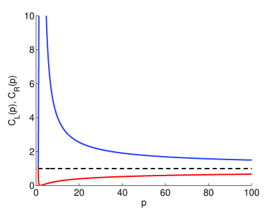
\psfrag{ReLambda}[b][b]{\footnotesize$\mathrm{Re}\,\lambda$}\psfrag{ImLambda}[b][b]{\footnotesize$\mathrm{Im}\,\lambda$}\psfrag{p1to2}[b][b]{\footnotesize{\color[rgb]{1,0,0}$1<p<2$}}\psfrag{p2toinfinity}[b][b]{\footnotesize{\color[rgb]{0,0,1}$2<p<\infty$}}\psfrag{phi}[b][b]{\footnotesize\hskip 5.69046pt$\left|\arg\lambda\right|=\cos^{-1}\left(\frac{\left|p-2\right|}{p}\right)$}\psfrag{Sigmap}[b][b]{\footnotesize{\color[rgb]{0,1,0}$\Sigma_{p}$}}\includegraphics[width=208.13574pt]{dissipativity.eps}

Figure 4.1. (a) $p$-dependent bounds $C_{L}$ (red) and $C_{R}$ (blue) for the spectral condition number of Hermitian positive definite matrices $A$, (b) conic section for the antieigenvalue assumption (A5) for normal accretive matrices $A$

4.4. $\boldsymbol{\mu_{1}(A)}$ for normal accretive matrices

If $A$ is a normal accretive matrix, then $\mu_{1}(A)$ from (3.4) is given by $\mu_{1}(A)=\min(E\cup F)$, where

$$E:= \left\{\left.\frac{a_{j}}{\left|\lambda_{j}^{A}\right|}\right|1\leqslant j\leqslant N\right\},$$

$$F:= \left\{\rule{0.0pt}{31.2982pt}\left.\frac{2\sqrt{\left(a_{j}-a_{i}\right)\left(a_{i}\left|\lambda_{j}^{A}\right|^{2}-a_{j}\left|\lambda_{i}^{A}\right|^{2}\right)}}{\left|\lambda_{j}^{A}\right|^{2}-\left|\lambda_{i}^{A}\right|^{2}}\right|\right.0<\frac{a_{j}\left|\lambda_{j}^{A}\right|^{2}-2a_{i}\left|\lambda_{j}^{A}\right|^{2}+a_{j}\left|\lambda_{i}^{A}\right|^{2}}{\left(\left|\lambda_{i}^{A}\right|^{2}-\left|\lambda_{j}^{A}\right|^{2}\right)\left(a_{i}-a_{j}\right)}<1,$$

$$\qquad\qquad\qquad\qquad\qquad\qquad\qquad\qquad\;\;\left.\rule{0.0pt}{31.2982pt}1\leqslant i,j\leqslant N,\,\left|\lambda_{i}^{A}\right|\neq\left|\lambda_{j}^{A}\right|\right\},$$

and $\lambda_{j}^{A}=a_{j}+ib_{j}$ with $a_{j},b_{j}\in\mathbb{R}$, $1\leqslant j\leqslant N$, denote the eigenvalues of $A$. In particular, if

(4.4) $$\mu_{1}(A)=\frac{a_{j}}{\left|\lambda_{j}^{A}\right|}\text{ for some $1\leqslant j\leqslant N$,}$$

then $\mu_{1}(A)=\frac{\mathrm{Re}\,\left\langle w,Aw\right\rangle}{|Aw|}$ for an antieigenvector $w\in\mathbb{K}^{N}$ with $\left|w_{j}\right|=1$ and $\left|w_{k}\right|=0$ for $1\leqslant k\leqslant N$ with $k\neq j$. Conversely, if

(4.5) $$\mu_{1}(A)=\frac{2\sqrt{\left(a_{j}-a_{i}\right)\left(a_{i}\left|\lambda_{j}^{A}\right|^{2}-a_{j}\left|\lambda_{i}^{A}\right|^{2}\right)}}{\left|\lambda_{j}^{A}\right|^{2}-\left|\lambda_{i}^{A}\right|^{2}}\text{ for some $1\leqslant i,j\leqslant N$ with $\left|\lambda_{i}^{A}\right|\neq\left|\lambda_{j}^{A}\right|$,}$$

then $\mu_{1}(A)=\frac{\mathrm{Re}\,\left\langle w,Aw\right\rangle}{|Aw|}$ for an antieigenvector $w\in\mathbb{K}^{N}$ with

$$\left|w_{i}\right|^{2}=\frac{a_{j}\left|\lambda_{j}^{A}\right|^{2}-2a_{i}\left|\lambda_{j}^{A}\right|^{2}+a_{j}\left|\lambda_{i}^{A}\right|^{2}}{\left(\left|\lambda_{i}^{A}\right|^{2}-\left|\lambda_{j}^{A}\right|^{2}\right)\left(a_{i}-a_{j}\right)},\quad\left|w_{j}\right|^{2}=\frac{a_{i}\left|\lambda_{i}^{A}\right|^{2}-2a_{j}\left|\lambda_{i}^{A}\right|^{2}+a_{i}\left|\lambda_{j}^{A}\right|^{2}}{\left(\left|\lambda_{i}^{A}\right|^{2}-\left|\lambda_{j}^{A}\right|^{2}\right)\left(a_{i}-a_{j}\right)}$$

and $\left|w_{k}\right|=0$ for $1\leqslant k\leqslant N$ with $k\neq i$ and $k\neq j$. This result can be found in [13, Theorem 5.1], [14, Theorem 3.1], [28, Theorem 1.1] and [26, Theorem 1]. The proof in [13, Theorem 5.1] is based on an application of the Lagrange multiplier method in order to solve a minimization problem. Furthermore, in [6] it was proved that the expression on the right hand side of (4.5) is an upper bound for $\mu_{1}(A)$. In [6] one can also find a geometric interpretation of this equality by a semi-ellipse.

If $\mu_{1}(A)$ is given by (4.4) for some $1\leqslant j\leqslant N$, then the $L^{p}$-antieigenvalue condition (A5) is equivalent to, compare (4.1),

(4.6) $$\frac{|p-2|}{2\sqrt{p-1}}\left|\mathrm{Im}\,\lambda_{j}^{A}\right|<\mathrm{Re}\,\lambda_{j}^{A},\;1<p<\infty.$$

This leads to a cone condition which postulates that every eigenvalues of $A$ is even contained in a $p$-dependent sector $\Sigma_{p}$ in the open right half-plane, called a conic section,

$$\Sigma_{p}:= \left\{\lambda\in\mathbb{C}\mid\frac{\left|p-2\right|}{2\sqrt{p-1}}\left|\mathrm{Im}\,\lambda\right|<\mathrm{Re}\,\lambda\right\}$$

$$= \left\{\lambda\in\mathbb{C}\mid\left|\arg\lambda\right|<\cos^{-1}\left(\frac{\left|p-2\right|}{p}\right)\right\},\,1<p<\infty,$$

see Figure 4.1(b). The opening angle $\left|\arg\lambda\right|$ is close to $0$ for small and large $p$, i.e. $p$ close to $1$ or $\infty$, and it is $\frac{\pi}{2}$ for $p=2$. Indeed, this is the same requirement as in the scalar complex case, compare (4.2) for $N=1$ and $b=p-2$. In particular, to satisfy the cone condition for arbitrary large $p$, the matrix $A$ must be of the form $A=\mathrm{diag}(a_{1},\ldots,a_{N})$ for some positive $a_{1},\ldots,a_{N}\in\mathbb{R}$.

If $\mu_{1}(A)$ is given by (4.5) for some $1\leqslant i,j\leqslant N$ with $\left|\lambda_{i}^{A}\right|\neq\left|\lambda_{j}^{A}\right|$, then the $L^{p}$-antieigenvalue condition (A5) is equivalent to

(4.7) $$\frac{2\sqrt{\left(a_{j}-a_{i}\right)\left(a_{i}\left|\lambda_{j}^{A}\right|^{2}-a_{j}\left|\lambda_{i}^{A}\right|^{2}\right)}}{\left|\lambda_{j}^{A}\right|^{2}-\left|\lambda_{i}^{A}\right|^{2}}>\frac{|p-2|}{p},\;1<p<\infty.$$

We emphasize the following equalities from [13, Section 6] and [6]

$$\frac{2\sqrt{\left(a_{j}-a_{i}\right)\left(a_{i}\left|\lambda_{j}^{A}\right|^{2}-a_{j}\left|\lambda_{i}^{A}\right|^{2}\right)}}{\left|\lambda_{j}^{A}\right|^{2}-\left|\lambda_{i}^{A}\right|^{2}}$$

$$= \frac{2\sqrt{\frac{|\lambda_{j}^{A}|}{|\lambda_{i}^{A}|}\left[\left(\frac{a_{i}}{|\lambda_{i}^{A}|}\right)\left(\frac{|\lambda_{j}^{A}|}{|\lambda_{i}^{A}|}\right)-\frac{a_{j}}{|\lambda_{j}^{A}|}\right]\left[\left(\frac{a_{j}}{|\lambda_{j}^{A}|}\right)\left(\frac{|\lambda_{j}^{A}|}{|\lambda_{i}^{A}|}\right)-\frac{a_{i}}{|\lambda_{i}^{A}|}\right]}}{\left(\frac{\left|\lambda_{j}^{A}\right|}{\left|\lambda_{i}^{A}\right|}\right)^{2}-1}$$

$$= \frac{2\sqrt{\left(r_{i}\rho_{ij}-r_{j}\right)\left(r_{j}\rho_{ij}-r_{i}\right)\rho_{ij}}}{\rho_{ij}^{2}-1},$$

where $\rho_{ij}:=\frac{|\lambda_{j}^{A}|}{|\lambda_{i}^{A}|}$ and $r_{k}:=\mathrm{Re}\,\frac{\lambda_{k}^{A}}{|\lambda_{k}^{A}|}=\frac{a_{k}}{|\lambda_{k}^{A}|}$ for $k=i,j$. This relation is helpful to verify, that all pairs of eigenvalues $\lambda_{j}^{A}$ and $\lambda_{i}^{A}$ satisfying (4.7) (under the constraint from the definition of $F$) must belong to a semi-ellipse, [6]. Moreover, note that in the scalar complex case with $A=\alpha\in\mathbb{C}$ we have $E=\left\{\frac{\mathrm{Re}\,\alpha}{|\alpha|}\right\}$, $F=\emptyset$, which implies $\frac{\mathrm{Re}\,\alpha}{|\alpha|}=\mu_{1}(\alpha)>\frac{|p-2|}{p}$. This is equivalent to (4.1) and also to (4.2).

4.5. $\boldsymbol{\mu_{1}(A)}$ for arbitrary matrices

If $A$ is an arbitrary matrix, there are only approximation results for $\mu_{1}(A)$. Such results are rather new in the literature and can be found in [27, Theorem 2]. However, for an arbitrary given matrix $A$ it is also possible to compute the first antieigenvalue and its corresponding antieigenvector directly. The computation of antieigenvalues and antieigenvectors has been analyzed in [25, 24].

References

- [1] W.-J. Beyn and J. Lorenz. Nonlinear stability of rotating patterns. Dyn. Partial Differ. Equ., 5(4):349–400, 2008.
- [2] A. Cialdea. Criteria for the -dissipativity of partial differential operators. In A. Cialdea, P. Ricci, and F. Lanzara, editors, Analysis, Partial Differential Equations and Applications, volume 193 of Operator Theory: Advances and Applications, pages 41–56. Birkhäuser Basel, 2009.
- [3] A. Cialdea. The -dissipativity of partial differential operators. Lect. Notes TICMI, 11:93, 2010.
- [4] A. Cialdea and V. Maz’ya. Criterion for the -dissipativity of second order differential operators with complex coefficients. J. Math. Pures Appl. (9), 84(8):1067–1100, 2005.
- [5] A. Cialdea and V. Maz′ya. Criteria for the -dissipativity of systems of second order differential equations. Ric. Mat., 55(2):233–265, 2006.
- [6] C. Davis. Extending the Kantorovic̆ inequality to normal matrices. Linear Algebra and its Applications, 31(0):173 – 177, 1980.
- [7] K. Gustafson. The angle of an operator and positive operator products. Bull. Amer. Math. Soc., 74:488–492, 1968.
- [8] K. Gustafson. Positive (noncommuting) operator products and semi-groups. Math. Z., 105:160–172, 1968.
- [9] K. Gustafson. Antieigenvalue inequalities in operator theory. In Inequalities, III (Proc. Third Sympos., Univ. California, Los Angeles, Calif., 1969; dedicated to the memory of Theodore S. Motzkin), pages 115–119. Academic Press, New York, 1972.
- [10] K. Gustafson. Antieigenvalues. Linear Algebra Appl., 208/209:437–454, 1994.
- [11] K. Gustafson. Operator trigonometry of iterative methods. Numer. Linear Algebra Appl., 4(4):333–347, 1997.
- [12] K. Gustafson. Antieigenvalue analysis : with applications to numerical analysis, wavelets, statistics, quantum mechanics, finance and optimization. World Scientific, Hackensack, NJ [u.a.], 2012.
- [13] K. Gustafson and M. Seddighin. Antieigenvalue bounds. J. Math. Anal. Appl., 143(2):327–340, 1989.
- [14] K. Gustafson and M. Seddighin. A note on total antieigenvectors. J. Math. Anal. Appl., 178(2):603–611, 1993.
- [15] K. E. Gustafson and D. K. M. Rao. Numerical range. Universitext. Springer-Verlag, New York, 1997. The field of values of linear operators and matrices.
- [16] R. A. Horn and C. R. Johnson. Matrix analysis. Cambridge Univ. Press, Cambridge [u.a.], 2. ed. edition, 2013.
- [17] M. G. Kreĭn. The angular localization of the spectrum of a multiplicative integral in Hilbert space. Funkcional. Anal. i Priložen., 3(1):89–90, 1969.
- [18] B. Mirman. Anti-eigenvalues: method of estimation and calculation. Linear Algebra Appl., 49:247–255, 1983.
- [19] D. Otten. Spatial decay and spectral properties of rotating waves in parabolic systems. PhD thesis, Bielefeld University, 2014, www.math.uni-bielefeld.de/~dotten/files/diss/Diss_DennyOtte%n.pdf. Shaker Verlag, Aachen.
- [20] D. Otten. Exponentially weighted resolvent estimates for complex Ornstein-Uhlenbeck systems. J. Evol. Equ., 2015.
- [21] D. Otten. The Identification Problem for complex-valued Ornstein-Uhlenbeck operators in . Sonderforschungsbereich 701, Preprint 14067, 2015 (submitted), https://www.math.uni-bielefeld.de/sfb701/files/preprints/sf%%****␣ANewAntieigenvalueCondition_DennyOtten_arxiv.tex␣Line␣1200␣****b14067.pdf.
- [22] K. Paul and G. Das. Symmetric antieigenvalues for normal operators. Int. J. Math. Anal. (Ruse), 4(9-12):509–525, 2010.
- [23] K. Paul, G. Das, and L. Debnath. Computation of antieigenvalues of bounded linear operators via centre of mass. arXiv:1007.4368v5, 2013.
- [24] M. Seddighin. Optimally rotated vectors. Int. J. Math. Math. Sci., (63):4015–4023, 2003.
- [25] M. Seddighin. Computation of antieigenvalues. Int. J. Math. Math. Sci., (5):815–821, 2005.
- [26] M. Seddighin. On the joint antieigenvalues of operators in normal subalgebras. J. Math. Anal. Appl., 312(1):61–71, 2005.
- [27] M. Seddighin. Approximations of antieigenvalue and antieigenvalue-type quantities. Int. J. Math. Math. Sci., pages Art. ID 318214, 15, 2012.
- [28] M. Seddighin and K. Gustafson. On the eigenvalues which express antieigenvalues. Int. J. Math. Math. Sci., (10):1543–1554, 2005.
- [29] G. E. Uhlenbeck and L. S. Ornstein. On the theory of the brownian motion. Phys. Rev., 36:823–841, Sep 1930.