Polynomial Finite Element Method for Domains Enclosed by Piecewise Conics

Abstract

We consider bivariate piecewise polynomial finite element spaces for curved domains bounded by piecewise conics satisfying homogeneous boundary conditions, construct stable local bases for them using Bernstein-Bézier techniques, prove error bounds and develop optimal assembly algorithms for the finite element system matrices. Numerical experiments confirm the effectiveness of the method.

1 Introduction

Spaces of multivariate piecewise polynomial splines are usually defined on triangulated polyhedral domains without imposing any boundary conditions. However, applications such as the finite element method require at least the ability to prescribe zero values on parts of the boundary. Fitting data with curved discontinuities of the derivatives is another situation where the interpolation of prescribed values along a lower dimensional manifold is highly desirable. It turns out that such conditions make the otherwise well understood spaces of e.g. bivariate $C^{1}$ macro-elements on triangulations significantly more complex. Even in the simplest case of a polygonal domain, the dimension of the space of splines vanishing on the boundary is dependent on its geometry, with consequences for the construction of stable bases (or stable minimal determining sets) [12, 13].

Since splines are piecewise polynomials, it is convenient to model curved features by piecewise algebraic surfaces so that the spline space naturally splits out the subspace of functions vanishing on such a surface. Indeed, implicit algebraic surfaces are a well-established modeling tool in CAGD [7], and the ability to exactly reproduce some of them (e.g. circles or cylinders) is a highly desirable feature for any modeling method [15].

On the other hand, the finite element analysis benefits a lot from the isogeometric approach [18], where the geometric models of the boundary are used exactly in the form they exist in a CAD system rather than undergoing a remeshing to fit into the traditional isoparametric finite element scheme. While the isogeometric analysis introduced in [18] is based on the most widespread modeling tool of NURBS and benefits from the many attractive features of tensor-product B-splines, it also inherits some of their drawbacks, such as complicated local refinement (see for example [10]).

In this paper we explore an isogeometric method which combines modeling with algebraic curves with the standard triangular piecewise polynomial finite elements in the simplest case of planar domains defined by piecewise quadratic algebraic curves (conic sections). Remarkably, the standard Bernstein-Bézier techniques for dealing with piecewise polynomials on triangulations [20, 22] as well as recent optimal assembly algorithms [2, 3, 4] for high order elements can be carried over to this case without significant loss of efficiency. Some of the material, especially in Sections 4 and 6 is based on the thesis [21] of one of the authors. Note that we only consider $C^{0}$ elements for elliptic problems with homogenous Dirichlet boundary conditions, although preliminary results on a direct implementation of non-homogenous Dirichlet boundary conditions can be found in [21].

In contrast to both the isoparametric curved finite elements and the isogeometric analysis, our approach does not require parametric patching on curved subtriangles, and therefore does not depend on the invertibility of the Jacobian matrices of the nonlinear geometry mappings. Therefore our finite elements remain piecewise polynomial everywhere in the physical domain. This in particular facilitates a relatively straightforward extention to $C^{1}$ elements on piecewise conic domains, which have also been considered in [21] and tested numerically on the approximate solution of fully nonlinear elliptic equations by Böhmer’s method [8]. Full details of the theory of these elements are postponed to our forthcoming paper [14].

There are some connections to the weighted extended B-spline (web-spline) method [17]. In particular, in our error analysis we use a technical lemma (Lemma 3.1) proved in [17]. Indeed, the quadratic polynomials that define the curved edges of the pie-shaped triangles at the domain boundary are factored out from the local polynomial spaces and hence act as weight functions on certain subdomains. They remain however integral parts of the spline spaces in our case and are generated naturally from the conic sections defining the domain, thus bypassing the problem of the computation of a smooth global weight function needed in the web-spline method.

The paper is organized as follows. We introduce in Section 2 the spaces $S_{d,0}(\triangle)$ of $C^{0}$ piecewise polynomials of degree $d$ on domains bounded by a number of conic sections, with homogeneous boundary conditions and investigate in Section 3 their approximation power for functions in Sobolev spaces $H^{m}(\Omega)$ vanishing on the boundary, which leads in particular to the error bounds in the form $\mathcal{O}(h^{m})$ in the $L_{2}$-norm and $\mathcal{O}(h^{m-1})$ in the $H^{1}$-norm for the solutions of elliptic problems by the Ritz-Galerkin finite element method. Section 4 is devoted to the development of a basis for $S_{d,0}(\triangle)$ of Bernstein-Bézier type important for a numerically stable and efficient implementation of the method. Some implementation issues specific for the curved elements are treated in Section 5, including the fast assembly of the system matrices. Finally, Section 6 presents several numerical experiments involving the Poisson problem on two different curved domains, as well as the circular membrane eigenvalue problem. The results confirm the effectiveness of our method both in $h$- and $p$-refinement settings.

2 Piecewise polynomials on piecewise conic domains

Let $\Omega\subset\mathbb{R}^{2}$ be a bounded curvilinear polygonal domain with $\Gamma=\partial\Omega=\bigcup_{j=1}^{n}\overline{\Gamma}_{j}$, where each $\Gamma_{j}$ is an open arc of an algebraic curve of at most second order ( i.e., either a straight line or a conic). For simplicity we assume that $\Omega$ is simply connected. Let $Z=\{z_{1},\ldots,z_{n}\}$ be the set of the endpoints of all arcs numbered counter-clockwise such that $z_{j},z_{j+1}$ are the endpoints of $\Gamma_{j}$, $j=1,\ldots,n$. (We set $z_{j+n}=z_{j}$.) Furthermore, for each $j$ we denote by $\omega_{j}$ the internal angle between the tangents $\tau^{+}_{j}$ and $\tau^{-}_{j}$ to $\Gamma_{j}$ and $\Gamma_{j-1}$, respectively, at $z_{j}$. We assume that $0<\omega_{j}\leq 2\pi$, and set $\omega:=\min\{\omega_{j}\,:\;1\leq j\leq n\}$.

Our goal is to develop an $H^{1}$-conforming finite element method with polynomial shape functions suitable for solving second order elliptic problems on curvilinear polygons of the above type.

Let $\triangle$ be a triangulation of $\Omega$,  i.e., a subdivision of $\Omega$ into triangles, where each triangle $T\in\triangle$ has at most one edge replaced with a curved segment of the boundary $\partial\Omega$, and the intersection of any pair of the triangles is either a common vertex or a common (straight) edge if it is non-empty. The triangles with a curved edge are said to be pie-shaped. Any triangle $T\in\triangle$ that shares at least one edge with a pie-shaped triangle is called a buffer triangle, and the remaining triangles are ordinary. We denote by $\triangle_{0}$, $\triangle_{B}$ and $\triangle_{P}$ the sets of all ordinary, buffer and pie-shaped triangles of $\triangle$, respectively. Thus,

$$\triangle=\triangle_{0}\cup\triangle_{B}\cup\triangle_{P}$$

is a disjoint union, see Figure 1. We emphasize that a triangle with only straight edges on the boundary of $\Omega$ does not belong to $\triangle_{P}$.

We denote by $\mathbb{P}_{d}$ the space of all bivariate polynomials of total degree at most $d$. For each $j=1,\ldots,n$, let $q_{j}\in\mathbb{P}_{2}$ be a polynomial such that $\Gamma_{j}\subset\{x\in\mathbb{R}^{2}\,:\;q_{j}(x)=0\}$. By multiplying $q_{j}$ by $-1$ if needed, we ensure that $\partial_{\nu_{x}}q_{j}(x)<0$ for all $x$ in the interior of $\Gamma_{j}$, where $\nu_{x}$ denotes the unit outer normal to the boundary at $x$, and $\partial_{a}:=a\cdot\nabla$ is the directional derivative with respect to a vector $a$. Hence, $q_{j}(x)$ is positive for points in $\Omega$ near the boundary segment $\Gamma_{j}$. We assume that $q_{j}\in\mathbb{P}_{1}$ or $q_{j}\in\mathbb{P}_{2}\setminus\mathbb{P}_{1}$ depending on whether $\Gamma_{j}$ is a straight interval or a genuine conic arc.

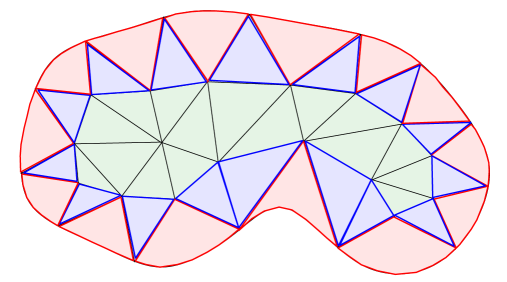
Figure 1: A triangulation of a curved domain with ordinary triangles (green), pie-shaped triangles (pink) and buffer triangles (blue).

Furthermore, let $V,E,V_{I},E_{I},V_{B}$ and $E_{B}$ denote the set of all vertices, all edges, interior vertices, interior edges, boundary vertices and boundary edges of $\triangle$, respectively. For each $v\in V$, $\operatorname{star}(v)$ stands for the union of all triangles in $\triangle$ attached to $v$. We also denote by $\theta$ the smallest angle of the triangles $T\in\triangle$, where the angle between an interior edge and a boundary segment is understood in the tangential sense.

We assume that $\triangle$ satisfies the following Conditions:

• $Z=\{z_{1},\ldots,z_{n}\}\subset V_{B}$.

• No interior edge has both endpoints on the boundary.

• If $q_{j}/q_{j-1}\neq\hbox{const}$ and at least one of $q_{j},q_{j-1}$ belongs to $\mathbb{P}_{2}\backslash\mathbb{P}_{1}$, then there is at least one triangle $T\in\triangle_{B}$ attached to $z_{j}$.

• Every $T\in\triangle_{P}$ is star-shaped with respect to its interior vertex $v$.

• For any $T\in\triangle_{P}$ with its curved side on $\Gamma_{j}$, $q_{j}(z)>0$ for all $z\in T\setminus\Gamma_{j}$.

Note that (b) and (c) can always be achieved by a slight modification of a given triangulation, while (d) and (e) hold for sufficiently fine triangulations.

For any $T\in\triangle$, let $h_{T}$ denote the diameter of $T$, and let $\rho_{T}$ be the radius of the disk $B_{T}$ inscribed in $T$ if $T\in\triangle_{0}\cup\triangle_{B}$ or in $T\cap T^{*}$ if $T\in\triangle_{P}$, where $T^{\ast}$ denotes the triangle obtained by joining the boundary vertices of $T$ by a straight line, see Figure 2. Note that every triangle $T\in\triangle$ is star-shaped with respect to $B_{T}$ in the sense of [9, Definition 4.2.2]. In particular, for $T\in\triangle_{P}$ this follows from Condition (d) and the fact that the conics do not possess inflection points.

\psfrag{R}{}\psfrag{A}{}\includegraphics[height=171.6869pt]{pieshapedT.eps} \psfrag{R}{}\psfrag{A}{}\psfrag{R}{}\psfrag{A}{}\includegraphics[height=171.6869pt]{pieshapedT2.eps}

Figure 2: A pie-shaped triangle with a curved edge and the associated triangle $T^{\ast}$ with straight sides and vertices $v_{1},v_{2},v_{3}$. The curved edge can be either outside (left) or inside $T^{\ast}$ (right).

We assume that $R,A,B$ are positive constants such that

$$h_{T}\leq R\rho_{T},\quad\forall T\in\triangle,$$ (1)

and, for any $T\in\triangle_{P}$,

$$q_{j}(z)\leq Aq_{j}(v),\quad\forall z\in T,$$ (2)

$$\partial_{v-z}q_{j}(z)\geq Bq_{j}(v),\quad\forall z\in T\cap\Gamma_{j},$$ (3)

where $\Gamma_{j}$ is the conic arc containing the curved edge of $T$, and $v$ is the interior vertex of $T$. The constants $R,A,B$ exist for any triangulation $\triangle$ of the above type and are responsible for the shape regularity of its triangles.

Let $d\geq 1$. We set

$$S_{d}(\triangle) :=\{s\in C^{0}(\Omega)\,:\;s|_{T}\in\mathbb{P}_{d+i},\;T\in\triangle_{i},\;i=0,1\},\quad\triangle_{1}:=\triangle_{P}\cup\triangle_{B},,$$

$$S_{d,0}(\triangle) :=\{s\in S_{d}(\triangle)\,:\;s|_{\Gamma}=0\}.$$

3 Error bounds

In this section we provide some typical error bounds for the spaces $S_{d,0}(\triangle)$ in the context of the approximation theory and the finite element method.

We denote by $\partial^{\alpha}f$, $\alpha\in\mathbb{Z}^{2}_{+}$, the partial derivatives of $f$ and consider the usual Sobolev spaces $H^{m}(\Omega)$ with the seminorm and norm defined by

$$|f|_{H^{m}(\Omega)}^{2}=\sum_{|\alpha|=m}\|\partial^{\alpha}f\|_{L^{2}(\Omega)}^{2},\quad\|f\|_{H^{m}(\Omega)}^{2}=\sum_{k=0}^{m}|f|_{H^{k}(\Omega)}^{2}\quad(H^{0}(\Omega)=L^{2}(\Omega)),$$

where $|\alpha|:=\alpha_{1}+\alpha_{2}$. We set $H^{1}_{0}(\Omega)=\{f\in H^{1}(\Omega):f|_{\partial\Omega}=0\}$.

3.1 Approximation error

Let $J_{1}$ be the set of all $j=1,\ldots,n$ such that $q_{j}\in\mathbb{P}_{1}$, and $J_{2}:=\{1,\ldots,n\}\setminus J_{1}$. For each $j\in J_{2}$ we choose a domain $\Omega_{j}\subset\Omega$ with Lipschitz boundary such that

• $\partial\Omega_{j}\cap\partial\Omega=\Gamma_{j}$,

• $\partial\Omega_{j}\setminus\partial\Omega$ is composed of a finite number of straight line segments,

• $q_{j}(x)>0$ for all $x\in\overline{\Omega}_{j}\setminus\Gamma_{j}$, and

• $\Omega_{j}\cap\Omega_{k}=\emptyset$ for all $j,k\in J_{2}$.

We assume that the triangulation $\triangle$ is such that for each $j\in J_{2}$,

$$\overline{\Omega}_{j} T\in\triangle_{P} \Gamma_{j}$$ contains every triangle whose curved edge is part of . (4)

Note that (4) will hold with the same set $\{\Omega_{j}:j\in J_{2}\}$ for any triangulations obtained by subdividing the triangles of $\triangle$. In addition we assume in this section for the sake of simplicity of the analysis that

no pair of pie-shaped triangles shares an edge. (5)

This can be achieved e.g. by applying Clough-Tocher splits [20, Section 6.2] to certain pie-shaped triangles. Finally, without loss of generality we assume that

$$\max_{x\in\overline{\Omega}_{j}}\|\nabla q_{j}(x)\|_{2}\leq 1,\text{ and }\|\nabla^{2}q_{j}\|_{2}\leq 1,\quad\text{for all }j\in J_{2},$$ (6)

which can always be achieved by appropriate renorming of $q_{j}$. (Here $\nabla^{2}q_{j}$ denotes the (constant) Hesse matrix of $q_{j}$.)

Lemma 3.1.

There is a constant $K$ depending only on $\Omega$, the choice of $\Omega_{j}$, $j\in J_{2}$, and $m\geq 1$, such that for all $j\in J_{2}$ and $u\in H^{m}(\Omega)\cap H^{1}_{0}(\Omega)$,

$$|u/q_{j}|_{H^{m-1}(\Omega_{j})}\leq K\|u\|_{H^{m}(\Omega_{j})}.$$ (7)

Proof. The lemma can be proved following the lines of the proof of [17, Theorem 6.1]. Indeed, $q_{j}$ is a smooth function and the only difference to the setting of that theorem is that $\Gamma_{j}$ is a proper part of the boundary of $\Omega_{j}$ rather than the full boundary. The argumentation in the proof however remains valid for this case.  

We define an operator $I_{\triangle}:H^{3}(\Omega)\cap H^{1}_{0}(\Omega)\to S_{d,0}(\triangle)$ of interpolatory type. For all $T\in\triangle_{0}\cup\triangle_{P}$ we set $I_{\triangle}u|_{T}=I_{T}(u|_{T})$, with the local operators $I_{T}$ defined as follows.

If $T\in\triangle_{0}$, then $I_{T}u$ is the polynomial of degree $d$ that interpolates $u$ on $D_{d,T}$, that is $I_{T}u\in\mathbb{P}_{d}$ is uniquely determined by the conditions $I_{T}u(\xi)=u(\xi)$ for all $\xi\in D_{d,T}$, see e.g. [20, Theorem 1.11].

Let $T\in\triangle_{P}$ with the curved edge on $\Gamma_{j}$. Denote by $T^{**}$ the (unique) triangle with straight edges such that $B_{T}\subset T^{**}\subset T$. (Note that $T^{**}=T^{*}$ if $T$ is convex.) Then $I_{T}u:=pq_{j}$, where $p\in\mathbb{P}_{d-1}$ interpolates $u/q_{j}$ on $D_{d-1,T^{**}}$. This interpolation scheme is well defined even though $T^{**}$ may include points on the boundary $\Gamma_{j}$ because $u/q_{j}\in H^{2}(\Omega_{j})$ by Lemma 3.1, and hence $u/q_{j}$ can be identified with a continuous function on $\overline{\Omega}_{j}$ by Sobolev embedding.

Finally, assume that $T\in\triangle_{B}$. Then $p:=I_{\triangle}u|_{T}\in\mathbb{P}_{d+1}$ is determined by the following interpolation conditions on $D_{d+1,T}$: $p(\xi)=u(\xi)$ if $\xi\in D^{0}_{d+1,T}$, and $p(\xi)=I_{T^{\prime}}u(\xi)$ if $\xi\in D_{d+1,T}\setminus D^{0}_{d+1,T}$, where $T^{\prime}$ is a triangle in $\triangle_{0}\cup\triangle_{P}$ containing the point $\xi$. The triangle $T^{\prime}$ is uniquely defined unless $\xi$ is the interior vertex of a pie-shaped triangle. In the latter case it is easy to check that $p(\xi)=u(\xi)$ independently of the choice of $T^{\prime}$, which shows that $p$ is well defined. This argument also shows that $I_{\triangle}u$ is continuous at the interior vertices of all pie-shaped triangles.

To see that $I_{\triangle}u\in S_{d,0}(\triangle)$ we need to demonstrate the continuity of $I_{\triangle}u$ across all interior edges of $\triangle$. If $e$ is the common edge of two triangles $T^{\prime},T^{\prime\prime}\in\triangle_{0}$, then the continuity follows from the standard argument that the restrictions $I_{T^{\prime}}u|_{e}$ and $I_{T^{\prime\prime}}u|_{e}$ coincide as univariate polynomials of degree $d$ satisfying identical interpolation conditions at $d+1$ points of $D_{d,T^{\prime}}\cap e=D_{d,T^{\prime\prime}}\cap e$. The same argument applies to the common edges of buffer triangles. Finally, the continuity of $I_{\triangle}u$ across edges shared by buffer triangles with either ordinary or pie-shaped triangles follows from the exact reproduction of univariate polynomials of degree at most $d+1$ by the interpolation polynomial $I_{\triangle}u|_{T}$ on the edges of a buffer triangle $T$.

Lemma 3.2.

Let $T\in\triangle_{P}$ and its curved edge $e\subset\Gamma_{j}$. Then

$$\|I_{T}u\|_{L^{\infty}(T)}\leq C_{1}h_{T}\|u/q_{j}\|_{L^{\infty}(T)}\quad\text{if }\;u\in H^{3}(\Omega)\cap H^{1}_{0}(\Omega),$$ (8)

where $C_{1}$ depends only on $d$ and $h_{T}/\rho_{T}$. Moreover, if $d\geq 2$ and $3\leq m\leq d+1$, then for any $u\in H^{m}(\Omega)\cap H^{1}_{0}(\Omega)$,

$$\|u-I_{T}u\|_{H^{k}(T)} \leq C_{2}h_{T}^{m-k}|u/q_{j}|_{H^{m-1}(T)},\quad k=0,\ldots,m-1,$$ (9)

$$\|u-I_{T}u\|_{L^{\infty}(T)} \leq C_{3}h_{T}^{m-1}|u/q_{j}|_{H^{m-1}(T)},$$ (10)

where $C_{2},C_{3}$ depend only on $d$ and $h_{T}/\rho_{T}$.

Proof. We will denote by $C$ various constants depending only on $d$, and by $\tilde{C}$ constants depending only on $d$ and $h_{T}/\rho_{T}$.

Assume that $u\in H^{3}(\Omega)\cap H^{1}_{0}(\Omega)$ and recall that by definition $I_{T}u=pq_{j}$, where $p\in\mathbb{P}_{d-1}$ interpolates $u/q_{j}$ on $D_{d-1,T^{**}}$. It is not difficult to derive from the proof of [20, Theorem 1.12] that

$$\|p\|_{L^{\infty}(T^{**})}\leq C\max_{\xi\in D_{d-1,T^{**}}}|p(\xi)|,$$ (11)

which implies

$$\|p\|_{L^{\infty}(T^{**})}\leq C\|u/q_{j}\|_{L^{\infty}(T^{**})}\leq C\|u/q_{j}\|_{L^{\infty}(T)}.$$

Since $T$ is star-shaped with respect to $B_{T}\subset T^{**}$, for any $x\in T$ the absolute value of the restriction of $p$ to the straight line through $x$ and the incenter $z_{T}$ of $T^{**}$ is bounded by $\|p\|_{L^{\infty}(T^{**})}$ inside $B_{T}$. By the well-known extremal property of the Chebyshev polynomial $T_{d-1}$ it follows that $|p(x)|\leq|T_{d-1}(\|x-z_{T}\|_{2}/\rho_{T})|\,\|p\|_{L^{\infty}(T^{**})}$, so that

$$\|p\|_{L^{\infty}(T)}\leq\tilde{C}\|p\|_{L^{\infty}(T^{**})},$$

with $\tilde{C}=|T_{d-1}(h_{T}/\rho_{T})|$. In view of (6), $\|q_{j}\|_{L^{\infty}(T)}\leq h_{T}$, and hence

$$\|I_{T}u\|_{L^{\infty}(T)}=\|pq_{j}\|_{L^{\infty}(T)}\leq h_{T}\|p\|_{L^{\infty}(T)},$$

which completes the proof of (8).

Since the area of $T$ is less or equal $\frac{\pi}{4}h^{2}_{T}$ and $\partial^{\alpha}(I_{T}u)\in\mathbb{P}_{d-k+1}$ if $|\alpha|=k$, it follows that

$$\|\partial^{\alpha}(I_{T}u)\|_{L^{2}(T)}\leq\frac{\sqrt{\pi}}{2}h_{T}\|\partial^{\alpha}(I_{T}u)\|_{L^{\infty}(T)}\leq\tilde{C}h_{T}\|\partial^{\alpha}(I_{T}u)\|_{L^{\infty}(T^{**})}.$$

By Markov inequality (see e.g. [20, Theorem 1.2]) we get furthermore

$$\|\partial^{\alpha}(I_{T}u)\|_{L^{\infty}(T^{**})}\leq\frac{C}{\rho_{T}^{k}}\|I_{T}u\|_{L^{\infty}(T^{**})},$$

and hence

$$|I_{T}u|_{H^{k}(T)}\leq\tilde{C}h^{1-k}_{T}\|I_{T}u\|_{L^{\infty}(T^{**})}.$$ (12)

In view of (8) we arrive at

$$|I_{T}u|_{H^{k}(T)}\leq\tilde{C}h^{2-k}_{T}\|u/q_{j}\|_{L^{\infty}(T)},\quad\text{if }\;u\in H^{3}(\Omega)\cap H^{1}_{0}(\Omega).$$ (13)

Let $d\geq 2$ and $3\leq m\leq d+1$, and let $u\in H^{m}(\Omega)\cap H^{1}_{0}(\Omega)$. It follows from Lemma 3.1 that $u/q_{j}\in H^{m-1}(T)$. By the results in [9, Chapter 4] there exists a polynomial $\tilde{p}\in\mathbb{P}_{m-2}$ such that

$$\|u/q_{j}-\tilde{p}\|_{H^{k}(T)} \leq\tilde{C}h_{T}^{m-k-1}|u/q_{j}|_{H^{m-1}(T)},\quad k=0,\ldots,m-1,\quad\text{and}$$

$$\|u/q_{j}-\tilde{p}\|_{L^{\infty}(T)} \leq\tilde{C}h_{T}^{m-2}|u/q_{j}|_{H^{m-1}(T)}.$$

Indeed, a suitable $\tilde{p}$ is given by the averaged Taylor polynomial [9, Definition 4.1.3] with respect to the disk $B_{T}$, and the inequalities in the last display follow from [9, Lemma 4.3.8] (Bramble-Hilbert Lemma) and [9, Proposition 4.3.2], respectively. (It is easy to check by inspecting the proofs in [9] that the quotient $d_{T}/\rho_{T}$ can be used in the estimates instead of the so-called chunkiness parameter used there.)

Since

$$u-I_{T}u=(u/q_{j}-\tilde{p})q_{j}-I_{T}(u-\tilde{p}q_{j}),$$

we have for any norm $\|\cdot\|$,

$$\|u-I_{T}u\|\leq\|(u/q_{j}-\tilde{p})q_{j}\|+\|I_{T}(u-\tilde{p}q_{j})\|.$$

In view of (6),

$$\|(u/q_{j}-\tilde{p})q_{j}\|_{L^{\infty}(T)}\leq h_{T}\|u/q_{j}-\tilde{p}\|_{L^{\infty}(T)}\leq\tilde{C}h_{T}^{m-1}|u/q_{j}|_{H^{m-1}(T)},$$

and for any $k=0,\ldots,m-1$,

$$\|(u/q_{j}-\tilde{p})q_{j}\|_{H^{k}(T)} \leq Ch_{T}\|u/q_{j}-\tilde{p}\|_{H^{k}(T)}+C\|u/q_{j}-\tilde{p}\|_{H^{k-1}(T)})$$

$$\leq\tilde{C}h_{T}^{m-k}|u/q_{j}|_{H^{m-1}(T)}.$$

Furthermore, by (8)

$$\|I_{T}(u-\tilde{p}q_{j})\|_{L^{\infty}(T)}\leq\tilde{C}h_{T}\|u/q_{j}-\tilde{p}\|_{L^{\infty}(T)}\leq\tilde{C}h_{T}^{m-1}|u/q_{j}|_{H^{m-1}(T)},$$

and by (13)

$$\|I_{T}(u-\tilde{p}q_{j})\|_{H^{k}(T)}\leq\tilde{C}h^{2-k}_{T}\|u/q_{j}-\tilde{p}\|_{L^{\infty}(T)}\leq\tilde{C}h^{m-k}_{T}|u/q_{j}|_{H^{m-1}(T)}.$$

By combining the inequalities in the five last displays we deduce (9) and (10).  

The approximation power of the space $S_{d,0}(\triangle)$ is estimated in the following theorem.

Theorem 3.3.

Let $d\geq 2$ and $3\leq m\leq d+1$. For any $u\in H^{m}(\Omega)\cap H^{1}_{0}(\Omega)$,

$$\inf_{s\in S_{d,0}(\triangle)}\|u-s\|_{H^{k}(\Omega)}\leq C_{4}h^{m-k}\|u\|_{H^{m}(\Omega)},\quad k=0,\ldots,m-1,$$ (14)

where $h$ is the maximum diameter of the triangles in $\triangle$, and $C_{4}$ is a constant depending only on $d$ and $R$, as well as on $\Omega$ and the choice of $\Omega_{j}$ for all $j\in J_{2}$.

Proof. We again use $C$ for various constants depending only on the parameters mentioned for $C_{4}$ in the formulation of the theorem. We show the error bound in (14) for $s=I_{\triangle}u$. For this sake we estimate the norms of $u-I_{T}u$ on all triangles $T\in\triangle$.

If $T\in\triangle_{0}$, then by [9, Theorem 4.4.4]

$$\|u-I_{T}u\|_{H^{k}(T)}\leq Ch_{T}^{m-k}|u|_{H^{m}(T)},\quad k=0,\ldots,m,$$ (15)

where $C$ depends only on $d$ and $h_{T}/\rho_{T}$. If $T\in\triangle_{P}$, with the curved edge $e\subset\Gamma_{j}$, then the estimate (9) holds by Lemma 3.2.

Let $T\in\triangle_{B}$, $p:=I_{\triangle}u|_{T}$ and let $\tilde{p}\in\mathbb{P}_{d+1}$ be the interpolation polynomial that satisfies $\tilde{p}(\xi)=u(\xi)$ for all $\xi\in D_{d+1,T}$. Then

$$\tilde{p}(\xi)-p(\xi)=\begin{cases}0&\text{if }\xi\in D^{0}_{d+1,T},\\ u(\xi)-I_{T^{\prime}}u(\xi)&\text{if }\xi\in D_{d+1,T}\setminus D^{0}_{d+1,T},\end{cases}$$

where $T^{\prime}\in\triangle_{0}\cup\triangle_{P}$ contains $\xi$. Hence, by the same arguments leading to (11) and (12) in the proof of Lemma 3.2, we conclude that for $k=0,\ldots,m$,

$$\|\tilde{p}-p\|_{H^{k}(T)} \leq Ch_{T}^{1-k}\|\tilde{p}-p\|_{L^{\infty}(T)}$$

$$\leq Ch_{T}^{1-k}\max\{\|u-I_{T^{\prime}}u\|_{L^{\infty}(T^{\prime})}:T^{\prime}\in\triangle_{0}\cup\triangle_{P},\;T^{\prime}\cap T\neq\emptyset\},$$

whereas by [9, Theorem 4.4.4] we have

$$\|u-\tilde{p}\|_{H^{k}(T)}\leq Ch_{T}^{m-k}|u|_{H^{m}(T)},$$

with the constants depending only on $d$ and $h_{T}/\rho_{T}$. If $T^{\prime}\in\triangle_{0}\cup\triangle_{P}$, then by [9, Corollary 4.4.7] and (10),

$$\|u-I_{T^{\prime}}u\|_{L^{\infty}(T^{\prime})}\leq Ch_{T^{\prime}}^{m-1}\begin{cases}|u|_{H^{m}(T^{\prime})}&\text{if }T^{\prime}\in\triangle_{0},\\ |u/q_{j}|_{H^{m-1}(T^{\prime})}&\text{if }T^{\prime}\in\triangle_{P},\end{cases}$$

where $C$ depends only on $d$ and $h_{T^{\prime}}/\rho_{T^{\prime}}$. By combining these inequalities we obtain an estimate of $\|u-p\|_{H^{k}(T)}$ by $C\tilde{h}^{m-k}$ times the maximum of $|u|_{H^{m}(T)}$, $|u|_{H^{m}(T^{\prime})}$ for $T^{\prime}\in\triangle_{0}$ sharing edges with $T$, and $|u/q_{j}|_{H^{m-1}(T^{\prime})}$ for $T^{\prime}\in\triangle_{P}$ sharing edges with $T$. Here $C$ depends only on $d$ and the maximum of $h_{T}/\rho_{T}$ and $h_{T^{\prime}}/\rho_{T^{\prime}}$, and $\tilde{h}$ is the maximum of $h_{T}$ and $h_{T^{\prime}}$ for $T^{\prime}\in\triangle_{0}\cup\triangle_{P}$ sharing edges with $T$.

By using (15) on $T\in\triangle_{0}$, (9) on $T\in\triangle_{P}$ and the estimate of the last paragraph on $T\in\triangle_{B}$, we get

$$\|u-I_{\triangle}u\|_{H^{k}(\Omega)}^{2} =\sum_{T\in\triangle}\|u-I_{\triangle}u\|_{H^{k}(T)}^{2}$$

$$\leq Ch^{2(m-k)}\Big{(}\sum_{T\in\triangle_{0}\cup\triangle_{B}}|u|_{H^{m}(T)}^{2}+\sum_{T\in\triangle_{P}}|u/q_{j(T)}|_{H^{m-1}(T)}^{2}\Big{)},$$

where $C$ depends only on $d$ and $R$, and $j(T)$ is the index of $\Gamma_{j}$ containing the curved edge of $T\in\triangle_{P}$. Clearly,

$$\sum_{T\in\triangle_{0}\cup\triangle_{B}}|u|_{H^{m}(T)}^{2}\leq|u|_{H^{m}(\Omega)}^{2},$$

whereas by Lemma 3.1,

$$\sum_{T\in\triangle_{P}}|u/q_{j(T)}|_{H^{m-1}(T)}^{2}\leq\sum_{j\in J_{2}}|u/q_{j}|_{H^{m-1}(\Omega_{j})}^{2}\leq K\|u\|_{H^{m}(\Omega)}^{2},$$

where $K$ is the constant of (7) depending only on $\Omega$ and the choice of $\Omega_{j}$, $j\in J_{2}$.  

3.2 Solution of elliptic problems

For simplicity we restrict ourselves to symmetric regular elliptic problems with homogeneous Dirichlet boundary conditions.

Consider the variational problem

find $$u\in H^{1}_{0}(\Omega) a(u,v)=(f,v) v\in H^{1}_{0}(\Omega)$$ such that for all , (16)

where $a(\cdot,\cdot)$ is a symmetric, bounded and coercive bilinear form (see e.g. [9] for the definitions), such that the regularity condition

$$\|u\|_{H^{2}(\Omega)}\leq C_{R}\|f\|_{L^{2}(\Omega)},$$ (17)

holds with some constant $C_{R}>0$ independent of $f$. Note that (17) holds for the domains considered in this work if $\omega_{j}\leq\pi$, $j=1,\ldots,n$, see e.g. [23, p. 158].

The finite element approximation $\tilde{u}$ of $u$ relying on the space $S_{d,0}(\triangle)$ is found as the solution of the discretized problem

find $$\tilde{u}\in S_{d,0}(\triangle) a(\tilde{u},s)=(f,s) s\in S_{d,0}(\triangle)$$ such that for all . (18)

The existence and uniqueness of the solutions of (16) and (18) follows by the well-known Lax-Milgram Theorem as soon as the bilinear form is coercive and bounded.

As a consequence of Theorem 3.3, we obtain the following error estimates by using the standard arguments in the finite element method, see the proofs of Theorems 5.4.4, 5.4.8 and 5.7.6 in [9].

Theorem 3.4.

Suppose that the variational problem (16) is symmetric, bounded, coercive and regular in the sense of (17). Let $d\geq 2$ and $3\leq m\leq d+1$. Then

$$\|u-\tilde{u}\|_{L^{2}(\Omega)}\leq C_{1}h^{m}\|u\|_{H^{m}(\Omega)},$$ (19)

$$\|u-\tilde{u}\|_{H^{1}(\Omega)}\leq C_{2}h^{m-1}\|u\|_{H^{m}(\Omega)},$$ (20)

where $h$ is the maximum diameter of the triangles in $\triangle$, and $C_{1},C_{2}$ are constants depending only on $\Omega$, $d$, $R$ and the choice of $\Omega_{j}$, $j\in J_{2}$.

4 Bernstein-Bézier basis

In order to treat elliptic problems with homogenous Dirichlet boundary conditions, we need to describe a suitable local basis for $S_{d,0}(\triangle)$. To this end we use the Bernstein-Bézier techniques and construct a stable minimal determining set (MDS) for $S_{d,0}(\triangle)$. The main idea is to factorize polynomials over pie-shaped triangles. As usual, we identify the functionals of the MDS with certain domain points, albeit not always in the standard way.

4.1 Bernstein polynomials

Let $T$ be a non-degenerate triangle in the plane with vertices $v_{1},v_{2},v_{3}$. The bivariate Bernstein polynomials with respect to $T$ are defined by

$$B_{ijk}^{d}(v):=\frac{d!}{i!j!k!}b_{1}^{i}b_{2}^{j}b_{3}^{k},\quad i+j+k=d,$$

where $b_{1},b_{2},b_{3}$ are the barycentric coordinates of $v$, that is the unique coefficients of the expansion $v=\sum_{i=1}^{3}b_{i}v_{i}$ with $\sum_{i=1}^{3}b_{i}=1$. Recall that Bernstein polynomials form a basis for $\mathbb{P}_{d}$ and have many useful properties for dealing with bivariate polynomials and piecewise polynomials, see [20]. In particular, every polynomial $p$ of degree $d$ can be written in the BB-form as

$$p=\sum_{i+j+k=d}c_{ijk}B_{ijk}^{d},$$ (21)

where $c_{ijk}$ are called the BB-coefficients of $p$.

The BB-form is stable in the sense that there is a constant $K>0$ depending only on $d$, such that

$$K\|c\|_{\infty}\leq\|p\|_{L^{\infty}(T)}\leq\|c\|_{\infty},\qquad\|c\|_{\infty}:=\max_{i+j+k=d}|c_{ijk}|.$$ (22)

It is often convenient to index Bernstein polynomials by the elements of the set

$$D_{d,T}:=\left\{\xi_{ijk}=\frac{iv_{1}+jv_{2}+kv_{3}}{d}:\;i+j+k=d,\;i,j,k\geq 0\right\}$$ (23)

of so-called domain points, such that $B_{\xi}^{d}:=B_{ijk}^{d}$ and $c_{\xi}:=c_{ijk}$ when $\xi=\xi_{ijk}\in D_{d,T}$.

In particular, it is easy to express the continuity of piecewise polynomials as follows. Given two triangles $T$ and $\tilde{T}$ sharing an edge $e$, let $p$ and $\tilde{p}$ be two polynomials of degree $d$ written in the BB-form

$$p=\sum_{\xi\in D_{d,T}}c_{\xi}B_{\xi}^{d}\quad\text{ and }\quad\tilde{p}=\sum_{\xi\in D_{d,\tilde{T}}}\tilde{c}_{\xi}\tilde{B}_{\xi}^{d},$$

where $B_{\xi}^{d}$ and $\tilde{B}_{\xi}^{d}$ are the Bernstein polynomials with respect to $T$ and $\tilde{T}$, respectively. Then $p$ and $\tilde{p}$ join continuously along $e$ if their BB-coefficients over $e$ coincide, i.e.

$$\tilde{c}_{\xi}=c_{\xi},\quad\text{ for all }\;\xi\in D_{d,T}\cap D_{d,\tilde{T}}$$ (24)

4.2 Minimal determining sets

A key concept for dealing with spline spaces using Bernstein-Bézier techniques is that of a stable local minimal determining set of domain points, see [20]. Our setting of curved domains requires a bit more general concept of a minimal determining set of functionals which we describe below.

Definition 4.1.

Let $S$ be a finite dimensional linear space and $S^{*}$ its dual space. A set $\Lambda\subset S^{*}$ is said to be a determining set for $S$ if for any $s\in S$

$$\lambda(s)=0\quad\forall\lambda\in\Lambda\quad\Longrightarrow\quad s=0,$$

and $\Lambda$ is a minimal determining set (MDS) for the space $S$ if there is no smaller determining set.

In other words, a determining set is a spanning set of linear functionals, and an MDS is a basis of $S^{*}$. Therefore, any MDS $\Lambda$ uniquely determines a basis

$$\{s_{\lambda}:\lambda\in\Lambda\}$$ (25)

of $S$ by duality, such that

$$\lambda(s_{\mu})=\delta_{\lambda,\mu},\qquad\lambda,\mu\in\Lambda,$$

and any spline $s\in S$ can be written uniquely in the form

$$s=\sum_{\lambda\in\Lambda}c_{\lambda}s_{\lambda},\quad\text{with }c_{\lambda}=\lambda(s)\in\mathbb{R}.$$

A minimal determining set serves as a set of degrees of freedom of the space $S$, as the value $\mu(s)$ of any functional $\mu\in S^{*}$ is uniquely determined by the values $\lambda(s)$ for all $\lambda\in\Lambda$. For example, if $S$ is a space of functions on a set $\Omega$ such that the point evaluation functionals $s(x)$, $x\in\Omega$, are well-defined, then the values $s(x)$ for all $x$ are determined by $\lambda(s)$, $\lambda\in\Lambda$.

We define the properties of locality and stability of an MDS for the spaces of piecewise polynomial splines.

Let $\triangle$ be a partition of a bounded domain $\Omega\subset\mathbb{R}^{n}$ into a finite number of cells $T\in\triangle$, where each $T$ is a closed set with dense interior, such that $\bigcup_{T\in\triangle}T=\overline{\Omega}$ and $T_{1}\cap T_{2}\subset\partial T_{1}\cap\partial T_{2}$ for any $T_{1},T_{2}\in\triangle$. A finite dimensional linear space $S$ of real valued functions defined on $\Omega$ is said to be a spline space with respect to a partition $\triangle$ if $s|_{T}$ is an $n$-variate algebraic polynomial for any $s\in S$ and any $T\in\triangle$. The maximal total degree of such polynomials is called the degree of the spline space and is denoted $d_{S}$.

The star of a set $A\subset\Omega$ with respect to a partition $\triangle$ is given by

$$\operatorname{star}(A):=\bigcup\{T\in\triangle:T\cap A\neq\emptyset\}.$$

For any positive integer $\ell$ we define the $\ell$-star of $A$ recursively as

$$\operatorname{star}^{1}(A):=\operatorname{star}(A),\quad\operatorname{star}^{\ell}(A):=\operatorname{star}(\operatorname{star}^{\ell-1}(A)),\quad\ell\geq 2.$$

It is easy to see that $B\cap\operatorname{star}^{\ell}(A)\neq\emptyset$ if and only if there exists a chain of cells $T_{1},\ldots,T_{\ell}\in\triangle$ such that $T_{1}\cap A\neq\emptyset$, $T_{\ell}\cap B\neq\emptyset$, and $T_{i}\cap T_{i+1}\neq\emptyset$ for all $i=1,\ldots,\ell-1$. It is easy to derive from this that

$$B\cap\operatorname{star}^{\ell}(A)\neq\emptyset\quad \Longleftrightarrow\quad A\cap\operatorname{star}^{\ell}(B)\neq\emptyset,\qquad A,B\subset\Omega,$$

$$T\subset\operatorname{star}^{\ell}(A)\quad \Longleftrightarrow\quad A\cap\operatorname{star}^{\ell-1}(T)\neq\emptyset,\qquad T\in\triangle,\quad A\subset\Omega,$$

$$T_{2}\subset\operatorname{star}^{\ell}(T_{1})\quad \Longleftrightarrow\quad T_{1}\subset\operatorname{star}^{\ell}(T_{2}),\qquad T_{1},T_{2}\in\triangle.$$

Given a spline space $S$, a set $\omega\subset\Omega$ is said to be a supporting set of a linear functional $\lambda\in S^{*}$ if

$$\lambda(s)=0\quad\text{for all $s$ such that $s|_{\omega}=0$}.$$ (26)

Note that a supporting set is not unique, and a minimal supporting set may not exists since the intersection of two supporting sets is not necessarily a supporting set. For example, if $S$ is a space of continuously differentiable splines on a triangulation $\triangle$, and $\lambda(s)$ is a partial derivative of $s$ evaluated at a vertex $v$ of $\triangle$, then every triangle attached to $v$ is a supporting set of $\lambda$, but their intersection is just $\{v\}$ and this is in general not a supporting set.

Given a spline space $S$ and an MDS $\Lambda$, we define for each $T\in\triangle$ the set

$$\Lambda_{T}:=\{\lambda\in\Lambda:T\subset\operatorname{supp}s_{\lambda}\},$$

where $\{s_{\lambda}:\lambda\in\Lambda\}$ is the basis of $S$ dual to $\Lambda$. Thus, $\lambda\in\Lambda_{T}$ if and only if for a spline $s\in S$, $s|_{T}$ depends on the coefficient $c_{\lambda}=\lambda(s)$. The number

$$\kappa_{\Lambda}:=\max_{T\in\triangle}|\Lambda_{T}|$$

is called the covering number of the MDS $\Lambda$.

Definition 4.2.

A minimal determining set $\Lambda$ for a spline space $S$ is said to be $\ell$-local if there is a family of supporting sets $\omega_{\lambda}$ of $\lambda\in\Lambda$ such that $\omega_{\lambda}\subset\operatorname{star}^{\ell}(T)$ for any $T\in\triangle$ such that $\lambda\in\Lambda_{T}$.

Lemma 4.3.

Let $\Lambda$ be an $\ell$-local MDS. Then for any $T\subset\operatorname{supp}s_{\lambda}$,

$$\omega_{\lambda}\subset\operatorname{star}^{\ell}(T)\quad\text{\rm and}\quad\operatorname{supp}s_{\lambda}\subset\operatorname{star}^{2\ell+1}(T).$$

Moreover, if $\omega_{\lambda}=T_{\lambda}\in\triangle$, then

$$\operatorname{supp}s_{\lambda}\subset\operatorname{star}^{\ell}(T_{\lambda}).$$

Proof. Clearly, the support of any spline, in particular $s_{\lambda}$, is a union of cells $T\in\triangle$. Let $T\subset\operatorname{supp}s_{\lambda}$. Then $\lambda\in\Lambda_{T}$ and hence $\omega_{\lambda}\subset\operatorname{star}^{\ell}(T)$. Therefore $T\subset\operatorname{star}^{\ell+1}(\omega_{\lambda})$. It follows that $\operatorname{supp}s_{\lambda}\subset\operatorname{star}^{\ell+1}(\omega_{\lambda})\subset\operatorname{star}^{2\ell+1}(T)$. If $\omega_{\lambda}=T_{\lambda}\in\triangle$, then $T_{\lambda}\subset\operatorname{star}^{\ell}(T)$ implies $T\subset\operatorname{star}^{\ell}(T_{\lambda})$, and hence $\operatorname{supp}s_{\lambda}\subset\operatorname{star}^{\ell}(T_{\lambda})$.  

As a consequence of this lemma we note that $\kappa_{\Lambda}$ is bounded by the product of the dimension of the polynomials of degree $d_{S}$ and the maximal possible number of cells in $\operatorname{star}^{2\ell+1}(T)$. Indeed, this product is an upper bound for the dimension of $S|_{\operatorname{star}^{2\ell+1}(T)}$, and hence for $|\Lambda_{T}|$ because all basis splines $s_{\lambda}$ with $\lambda\in\Lambda_{T}$ are zero outside of $\operatorname{star}^{2\ell+1}(T)$ and therefore must be linearly independent within this set.

We now assume that $\Lambda$ is an $\ell$-local MDS for a spline space $S$, and $\{\omega_{\lambda}:\lambda\in\Lambda\}$ is the corresponding family of supporting sets. According to (26), $\lambda(s)$ is completely determined by the restricted spline $s|_{\omega_{\lambda}}$, which means that it can be considered as a bounded linear functional on the space $S|_{\omega_{\lambda}}=\{s|_{\omega_{\lambda}}:s\in S\}$, and so there is a constant $K_{1}\in(0,\infty)$ such that

$$|\lambda(s)|\leq K_{1}\|s\|_{L^{\infty}(\omega_{\lambda})}\quad\text{for all }\lambda\in\Lambda,\;s\in S.$$ (27)

In view of the definition of $\Lambda_{T}$, $s|_{T}=0$ if $\lambda(s)=0$ for all $\lambda\in\Lambda_{T}$. Hence $\max_{\lambda\in\Lambda_{T}}|\lambda(s)|$ is a norm on the space $S|_{T}$ and, in view of the equivalence of all norms on a finite-dimensional space, there exists a constant $K_{2}\in(0,\infty)$ such that

$$\|s\|_{L^{\infty}(T)}\leq K_{2}\max_{\lambda\in\Lambda_{T}}|\lambda(s)|\quad\text{for all }T\in\triangle,\;s\in S.$$ (28)

We call any constants $K_{1},K_{2}$ satisfying (27) and (28), respectively, the stability constants of the MDS $\Lambda$.

Proposition 4.4.

Let $\Lambda$ be an MDS for a spline space $S$. Then for any $a=\{a_{\lambda}\}_{\lambda\in\Lambda}\subset\mathbb{R}$,

$$K_{1}^{-1}\|a\|_{\infty}\leq\|\sum_{\lambda\in\Lambda}a_{\lambda}s_{\lambda}\|_{L^{\infty}(\Omega)}\leq\kappa_{\Lambda}K_{2}\|a\|_{\infty},$$

with $\|a\|_{\infty}:=\max_{\lambda\in\Lambda}|a_{\lambda}|$. Moreover, for any $1\leq p<\infty$,

$$\|\sum_{\lambda\in\Lambda}a_{\lambda}s^{(p)}_{\lambda}\|_{L^{p}(\Omega)}\leq\kappa_{\Lambda}^{1-1/p}K_{2}\|a\|_{p}$$

where

$$s^{(p)}_{\lambda}:=|\operatorname{supp}s_{\lambda}|^{-1/p}s_{\lambda},\qquad\|a\|_{p}:=\Big{(}\sum_{\lambda\in\Lambda}|a_{\lambda}|^{p}\Big{)}^{1/p}.$$

Proof. Let $s=\sum_{\lambda\in\Lambda}a_{\lambda}s_{\lambda}$. By (27), $|a_{\lambda}|=|\lambda(s)|\leq K_{1}\|s\|_{L^{\infty}(\Omega)}$, which implies the first inequality. On the other hand, for any $T\in\triangle$, since $\|s_{\lambda}\|_{L^{\infty}(\Omega)}\leq K_{2}$ by (28),

$$\|s|_{T}\|_{L^{\infty}(T)}=\|\sum_{\lambda\in\Lambda_{T}}a_{\lambda}s_{\lambda}\|_{L^{\infty}(T)}\leq\kappa_{\Lambda}\max_{\lambda\in\Lambda_{T}}\|a_{\lambda}s_{\lambda}\|_{L^{\infty}(T)}\leq\kappa_{\Lambda}K_{2}\|a\|_{\infty},$$

which completes the proof in the case $p=\infty$.

Let now $1\leq p<\infty$ and $s=\sum_{\lambda\in\Lambda}a_{\lambda}s^{(p)}_{\lambda}$. Then for any $T\in\triangle$,

$$\|s|_{T}\|^{p}_{L^{p}(T)}=\|\sum_{\lambda\in\Lambda_{T}}a_{\lambda}s^{(p)}_{\lambda}\|^{p}_{L^{p}(T)}\leq\kappa_{\Lambda}^{p-1}\sum_{\lambda\in\Lambda_{T}}\|a_{\lambda}s^{(p)}_{\lambda}\|^{p}_{L^{p}(T)}.$$

Hence

$$\|s\|^{p}_{L^{p}(\Omega)}=\sum_{T\in\triangle}\|s|_{T}\|^{p}_{L^{p}(T)}\leq\kappa_{\Lambda}^{p-1}\sum_{\lambda\in\Lambda}|a_{\lambda}|^{p}\sum_{T\in\triangle\atop T\subset\operatorname{supp}s_{\lambda}}\|s^{(p)}_{\lambda}\|^{p}_{L^{p}(T)}\leq\kappa_{\Lambda}^{p-1}K_{2}\|a\|^{p}_{p},$$

where we have taken into account that $\|s_{\lambda}\|_{L^{p}(\Omega)}\leq K_{2}|\operatorname{supp}s_{\lambda}|^{1/p}$ in view of (28). This implies the second statement.  

This proposition shows that $\kappa_{\Lambda}K_{1}K_{2}$ is an upper bound for the $L_{\infty}$-stability constant of the basis $\{s_{\lambda}\}_{\lambda\in\Lambda}$. For $p<\infty$, the lower $L_{p}$-stability estimates of the form

$$CK_{1}^{-1}\|a\|_{p}\leq\|\sum_{\lambda\in\Lambda}a_{\lambda}s^{(p)}_{\lambda}\|_{L^{p}(\Omega)}$$

with some $C>0$ are more complicated. Under additional assumptions on the partition $\triangle$, they hold with $C$ depending only on $\ell$, $n$ and $d_{S}$, see e.g. [11, Lemma 6.2] and [20, Theorem 5.22].

This motivates the following definition.

Definition 4.5.

A family of minimal determining sets $\Lambda_{i}$, $i\in\mathcal{I}$, for given spline spaces $S_{i}$, $i\in\mathcal{I}$, is said to be stable and local if there exist $\ell$, $\kappa$, $K_{1}$ and $K_{2}$ such that every $\Lambda_{i}$ is $\ell$-local, the covering numbers satisfy $\kappa_{\Lambda_{i}}\leq\kappa$, $i\in\mathcal{I}$, and (27) and (28) hold for all $\Lambda_{i}$ with the same stability constants $K_{1},K_{2}$.

Typically such a stable and local family of minimal determining sets is produced by an algorithm that generates an MDS for a specific type of splines on arbitrary regular triangulations in 2D or 3D, see [20]. With some abuse of terminology we say in this case that the MDS (given by an algorithm) is stable and local. The parameters $\ell,\kappa,K_{1},K_{2}$ usually depend only on the maximum degree of polynomials in $S|_{T}$ and on a shape regularity measure of the cells, such as the minimum angle of the triangles $T\in\triangle$ in the 2D case.

We now consider the special case when $\triangle$ is a triangulation of a bounded polygonal domain $\Omega\subset\mathbb{R}^{2}$, that is each cell $T$ is a triangle, and the intersection of two different triangles is their common vertex or edge if not empty. Let

$$D_{d,\triangle}:=\bigcup_{T\in\triangle}D_{d,T},$$

where $D_{d,T}$ is the set of domain points (23) for a single triangle. In view of (21) every continuous piecewise polynomial spline $s$ of degree $d$ with respect to $\triangle$ can be uniquely represented over each $T\in\triangle$ as

$$s|_{T}=\sum_{\xi\in D_{d,T}}c_{\xi}B_{\xi}^{T,d},$$

where $B_{\xi}^{T,d}$ are BB-basis polynomials of degree $d$ associated with the triangle $T$. In view of (24), the continuity of $s$ implies that the BB-vectors of $s|_{T}$ and $s|_{\tilde{T}}$ agree on domain points on the edge shared by triangles $T$ and $\tilde{T}$. Therefore each domain point $\xi\in D_{d,\triangle}$ defines on the space $S^{0}_{d}(\triangle)$ of all continuous splines of degree $d$ a linear functional $\gamma_{\xi}$ that picks the BB-coefficient $c_{\xi}$ of $s|_{T}$ for a triangle $T$ containing $\xi$. It is easy to see that

$$\Gamma:=\{\gamma_{\xi}:\xi\in D_{d,\triangle}\}$$

is a minimal determining set for $S^{0}_{d}(\triangle)$ [20, Section 5.4]. Minimal determining sets for many subspaces of $S^{0}_{d}(\triangle)$ can be obtained as subsets of $\Gamma$, which are conveniently identified with the corresponding subsets of $D_{d,\triangle}$, see [20].

It is easy to see that a supporting set of $\gamma_{\xi}$ is given by any triangle $T\in\triangle$ that contains $\xi$. However, $\{\xi\}$ is a supporting set if $\xi$ is a vertex of $\triangle$, and an edge $e$ of $\triangle$ is a supporting set if $\xi\in e$. Hence, our generalized definition of a local MDS (Definition 4.2) reduces to that given in [20, Definition 5.16], and the parameter $\ell$ is the same if we always take a triangle $T_{\xi}$ containing $\xi$ as a supporting set. Furthermore, [20, Theorem 2.6] shows that (27) is satisfied for each $\gamma_{\xi}$ with the triangle $T_{\xi}$ as a supporting set, and $K_{1}$ depending only on $d$, and (28) is equivalent to the condition [20, Eq. (5.13)]. Therefore, our notion of a stable local MDS (Definition 4.5) coincides with [20, Definition 5.16] in the case when the linear functionals belong to $\Gamma$. Similarly, stable local nodal minimal determining sets of [20, Section 5.9] are special cases of stable local MDS as defined in Definition 4.5.

4.3 A stable MDS and stable local basis for $S_{d,0}(\triangle)$

For each $T\in\triangle_{P}$, with its curved edge $e$ given by the equation $q(x)=0$, where the quadratic polynomial is normalized so that

$$q(v)=1\quad\text{for the interior vertex $v$ of $T$,}$$ (29)

we consider the space

$$q\mathbb{P}_{d-1}=\{pq\,:\;p\in\mathbb{P}_{d-1}\}\subset\mathbb{P}_{d+1}.$$

Recall that by Bézout theorem every polynomial that vanishes on the conic $q(x)=0$ is divisible by $q$, and thus $\mathbb{P}_{d-1}q$ consists of all polynomials of degree $d+1$ that vanish on $e$, that is

$$q\mathbb{P}_{d-1}=\{p\in\mathbb{P}_{d+1}\,:\;p|_{e}=0\}.$$

Since the BB polynomials $B_{ijk}^{d-1}$, $i+j+k=d-1$, w.r.t. $T^{\ast}$ form a basis for $\mathbb{P}_{d-1}$ it is obvious that the set

$$\left\{qB_{ijk}^{d-1}\,:\;i+j+k=d-1\right\}$$

is a basis for $q\mathbb{P}_{d-1}$. The set of domain points of degree $d-1$ over $T^{\ast}$ will be denoted $D^{\ast}_{d-1,T}$. Even though the set $D^{\ast}_{d-1,T}$ formally coincides with $D_{d-1,T^{\ast}}$, the linear functionals associated with the domain points are slightly different. Namely, each $\xi\in D^{\ast}_{d-1,T}$ represents a linear functional $\lambda_{\xi}$ on $S_{d,0}(\triangle)$ which picks the coefficient $c_{\xi}$ in the expansion

$$s|_{T}=q\sum_{\xi\in D^{\ast}_{d-1,T}}c_{\xi}B_{\xi}^{d-1},\qquad s\in S_{d,0}(\triangle).$$

Clearly, $s|_{T}\in q\mathbb{P}_{d-1}\subset\mathbb{P}_{d+1}$ may also be expressed in terms of BB polynomials $B_{\xi}^{d+1}$, $\xi\in D_{d+1,T^{\ast}}$, of degree $d+1$. Figure 3 depicts both sets of domain points for a pie-shaped triangle $T$ in the case $d=5$.

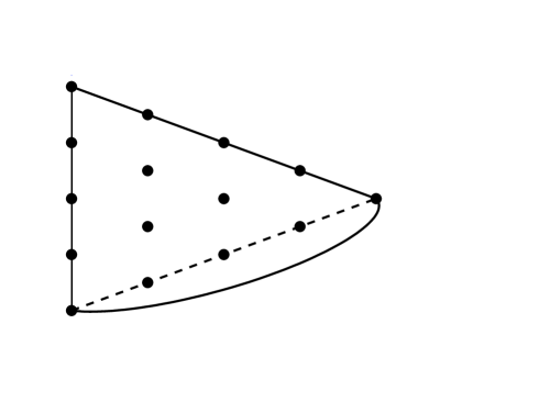
Figure 3: The sets $D^{\ast}_{d-1,T}$ (left) and $D_{d+1,T^{\ast}}$ (right) for $d=5$ over a pie-shaped triangle.

For the ordinary triangles $T\in\triangle_{0}$ we consider the usual sets of domain points $D_{d,T}$ (and corresponding functionals $\lambda_{\xi}=\gamma_{\xi}$) whose union $D_{d,\triangle_{0}}=\cup_{T\in\triangle_{0}}D_{d,T}$ forms the standard set of domain points associated with the subtriangulation $\triangle_{0}$ of $\triangle$.

Finally, for each buffer triangle $T:=\left\langle v_{1},v_{2},v_{3}\right\rangle\in\triangle_{B}$, let $D_{d+1,T}^{0}$ be the subset of $D_{d+1,T}$ obtained by removing all domain points on those edges of $T$ that are shared with triangles in either $\triangle_{0}$ or $\triangle_{P}$, see Figure 4.

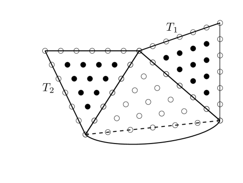
Figure 4: The points in $D^{0}_{d+1,T_{1}}\cup D^{0}_{d+1,T_{2}}$ for two buffer triangles $T_{1},T_{2}\in\triangle_{B}$ are marked by black dots ($d=5$).

We will need the following statement that shows that the division by $q$ on a pie-shaped triangle is stable.

Lemma 4.6.

Let $T\in\triangle_{P}$ with the curved edge $e$ of $T$ given by the equation $q(x)=0$, where $q=q_{j}/q_{j}(v)$ for some $j\in\{1,\ldots,n\}$, and $v$ is the interior vertex of $T$. Then for any $r\in\mathbb{P}_{d-1}$,

$$\|r\|_{L^{\infty}(T)}\leq C\|rq\|_{L^{\infty}(T)},$$

where the constant $C>0$ depends only on $d$ and $B$.

Proof. For any $z\in e$, consider the univariate polynomials $\tilde{r}(t)=r(tv+(1-t)z)$ and $\tilde{q}(t)=q(tv+(1-t)z)$, $t\in[0,1]$. Then $\tilde{q}(0)=0$ and $\tilde{q}^{\prime}(0)=\partial_{v-z}q(z)\geq B$ by (3). Hence $\tilde{q}(t)=t(at+b)$, with $b\geq B$. Since $\tilde{q}(1)=1$, we get $a+b=1$ and hence

$$at+b\geq\min\{B,1\},\qquad t\in[0,1].$$

We note for the later use in the proof of Lemma 3.1 that $\tilde{q}^{\prime}(t)=2at+b$ and hence $\partial_{v-z}q(v)=\tilde{q}^{\prime}(1)=2a+b=a+1$.

Let $\tilde{r}(t)=\sum_{i=0}^{d-1}a_{i}t^{i}$. In view of the equivalence of all norms on the space of univariate polynomials of a fixed degree, there exist constants $c_{1},c_{2}>0$ depending only on $d$ such that

$$c_{1}\max_{t\in[0,1]}\Big{|}\sum_{i=0}^{d-1}a_{i}t^{i}\Big{|}\leq\max_{0\leq i\leq d-1}|a_{i}|\leq c_{2}\max_{t\in[0,1]}\Big{|}\sum_{i=0}^{d-1}a_{i}t^{i+1}\Big{|}$$

and hence

$$\|\tilde{r}\tilde{q}\|_{L^{\infty}(0,1)}\geq\min\{B,1\}\max_{t\in[0,1]}\Big{|}\sum_{i=0}^{d-1}a_{i}t^{i+1}\Big{|}\geq\frac{c_{1}}{c_{2}}\min\{B,1\}\,\|\tilde{r}\|_{L^{\infty}(0,1)}.$$

The lemma follows because $T=\bigcup_{z\in e}[z,v]$.  

We are ready to formulate and prove the main result of this section.

Theorem 4.7.

Let

$$M_{0}:=\Big{(}D_{d,\triangle_{0}}\setminus\partial\Omega\Big{)}\cup\bigcup_{T\in\triangle_{P}}D_{d-1,T}^{\ast}\cup\bigcup_{T\in\triangle_{B}}D_{d+1,T}^{0}.$$ (30)

Then $M_{0}$ is a stable local minimal determining set for the space $S_{d,0}(\triangle)$ with $\ell=1$, $\kappa$ depending only on $d$, $K_{1}$ depending only on $d$ and $B$, and $K_{2}$ depending only on $d$ and $A$.

Proof. It is easy to see that all functionals in $M_{0}$ are well defined. In particular, if $\xi$ is the interior vertex $v$ of a pie-shaped triangle $T$ with the curved edge given by $q(x)=0$ satisfying (29), then the coefficient associated with $v$ is $c_{v}=s(v)$ regardless of whether we consider $v$ as an element of $D^{*}_{d-1,T}$ or an element of $D_{d,\triangle_{0}}$.

For any $\xi\in M_{0}$ we choose a triangle $T_{\xi}\in\triangle$ such that $\xi\in T_{\xi}$, where we make sure that $T_{\xi}\in\triangle_{0}$ if $\xi\in D_{d,\triangle_{0}}\setminus\partial\Omega$ and $T_{\xi}\in\triangle_{P}$ if $\xi\in\Big{(}\bigcup_{T\in\triangle_{P}}D_{d-1,T}^{\ast}\Big{)}\setminus D_{d,\triangle_{0}}$. Note that for $\xi\in\bigcup_{T\in\triangle_{B}}D_{d+1,T}^{0}$ there is always just one triangle $T_{\xi}\in\triangle$ that contains $\xi$, and it belongs to $\triangle_{B}$. If $T_{\xi}\in\triangle_{0}\cup\triangle_{B}$, then $|\lambda_{\xi}(s)|\leq C\|s\|_{L^{\infty}(T_{\xi})}$ for all $s\in S_{d,0}(\triangle)$ by [20, Theorem 2.6], where $C$ depends only on $d$. Assume that $T_{\xi}\in\triangle_{P}$ with the curved side of $T_{\xi}$ given by $q(x)=0$, and $s\in S_{d,0}(\triangle)$. Then $s|_{T_{\xi}}=qr$ for some $r\in\mathbb{P}_{d-1}$, and by the same results of [20] and Lemma 4.6, $|\lambda_{\xi}(s)|\leq C^{\prime}\|r\|_{L^{\infty}(T_{\xi})}\leq C\|s\|_{L^{\infty}(T_{\xi})}$, with a constant $C$ depending only on $d$ and $B$. Hence $T_{\xi}$ is a supporting set of the functional $\lambda_{\xi}$ satisfying (27) with a constant $K_{1}$ depending only on $d$ and $B$.

To show that $M_{0}$ is a minimal determining set and satisfies (28) with some uniform constant $K_{2}$, we follow the usual approach (see [20]) of setting the values $c_{\xi}=\lambda_{\xi}(s)$, $\xi\in M_{0}$, for any spline $s\in S_{d,0}(\triangle)$ and showing that the BB-coefficients of $s|_{T}$ for all $T\in\triangle$ can be computed from them consistently and stably.

If $T\in\triangle_{0}$, then the BB-coefficients of $s|_{T}$ are $c_{\xi}$ for $\xi\in M_{0}\cap T=D_{d,T}\setminus\partial\Omega$, and zeros for $\xi\in D_{d,T}\cap\partial\Omega$, so that no computation is needed.

If $T\in\triangle_{P}$, then the BB-coefficients of $s|_{T}$ can be computed by the multiplication of the BB-form of degree $d-1$ by the BB-form of the quadratic polynomial $q$, see the explicit formulas (35) below. In view of (2) and (22), we have $\|s|_{T}\|_{L^{\infty}(T)}\leq A\max_{\xi\in D_{d-1,T}^{\ast}}|\lambda_{\xi}(s)|$, and the BB-coefficients of $s|_{T}$ are bounded by $\|s|_{T}\|_{L^{\infty}(T)}$ times a constant depending only on $d$. Note that $D_{d-1,T}^{\ast}\cap(D_{d,\triangle_{0}}\setminus\partial\Omega)=\{v\}$, where $v$ is the interior vertex of $T$. Since $q(v)=1$, we see that the functional $\lambda_{v}(s)=s(v)$ is well-defined regardless of whether we associate it with $v$ as element of $D_{d-1,T}^{\ast}$ or $D_{d,\triangle_{0}}\setminus\partial\Omega$. Hence the BB-coefficient $s(v)$ of $s|_{T}$ at $v$ is computed consistently. If $T$ shares an interior edge $e$ with another pie-shaped triangle $T^{\prime}$, then Condition (c) of Section 2 implies that the curved edges of both $T$ and $T^{\prime}$ are given by the same equation $q(x)=0$. Therefor the BB-coefficients of $s$ for domain points in $D_{d-1,T}^{\ast}\cap D_{d-1,T^{\prime}}^{\ast}$ on the common edge of $T$ and $T^{\prime}$ are computed consistently by using the formulas (35) on either $T$ or $T^{\prime}$.

For a buffer triangle $T\in\triangle_{B}$ it is easy to see that the coefficients $c_{\xi}=\lambda_{\xi}(s)$, $\xi\in D_{d+1,T}^{0}$ give us the interior part of the Bézier net of the patch $s|_{T}$, as well as the BB-coefficients on any edges shared with other buffer triangles. Any BB-coefficients of $s|_{T}$ at the domain points on the boundary of $\Omega$ are zero, and those on the edges shared with pie-shaped triangles have been computed already. If the edge $e$ of $T$ is shared with a triangle $T^{\prime}\in\triangle_{0}$, then $s|_{e}$ has already been determined as the restriction of the polynomial $s|_{T^{\prime}}$ of degree $d$. Therefore we can obtain the BB-coefficients of $s|_{T}$, as a polynomial of degree $d+1$, for domain points in $e$ by the standard degree raising formulas [20, Section 2.15], which is a stable process.

Thus, we have shown that $M_{0}$ is a minimal determining set. For each $\xi\in M_{0}$, let $s_{\xi}$ denote the corresponding dual basis function in $S_{d,0}(\triangle)$. By inspecting the above arguments it is easy to see that

$$\operatorname{supp}s_{\xi}=\cup\{T\in\triangle:\xi\in T\}$$

(In particular, (35) shows that for $\xi$ in the interior of a pie-shaped triangle $T$ the BB-coefficients of $s_{\xi}|_{T}$ on the edges shared with buffer triangles are zero.) Hence

$$\Lambda_{T}=T\cap M_{0}\quad\text{for all}\;T\in\triangle,$$

which shows that $M_{0}$ is 1-local according to Definition 4.2, with the supporting sets $T_{\xi}$ described above. It is easy to see that $|\Lambda_{T}|\leq{d+2\choose 2}$ if $T\in\triangle_{0}$, $|\Lambda_{T}|={d+1\choose 2}$ if $T\in\triangle_{P}$, and $|\Lambda_{T}|\leq{d+2\choose 2}+d-2$ if $T\in\triangle_{B}$, which implies the following bound for the covering number:

$$\kappa_{\Lambda}\leq{d+2\choose 2}+d-2.$$

By inspecting again the above argumentation that $M_{0}$ is a minimal determining set we conclude that (28) is satisfied with $K_{2}$ depending only on $d$ and the constant $A$ of (2).  

The following statement about corresponding basis (25) follows immediately.

Corollary 4.8.

The dual basis functions $s_{\xi}:\xi\in M_{0}$ defined by the condition $\lambda_{\xi}(s_{\zeta})=\delta_{\xi\zeta}$ have local support and satisfy the stability estimates of Proposition 4.4 with constants depending only on $d,A,B$.

5 Implementation of the FEM

In this section we briefly discuss the implementation aspects of the finite element method for solving second order elliptic problems on piecewise conic domains using the Bernstein-Bézier basis of the previous section.

5.1 The conics

A convenient method to represent the piecewise conic boundary is provided by the rational Bézier curves. Given three control points $P_{0},{P}_{1},{P}_{2}\in\mathbb{R}^{2}$, the quadratic rational Bézier curve can be described by

$$B(t)=\frac{P_{0}B_{0}^{2}(t)+\beta{P}_{1}B_{1}^{2}(t)+{P}_{2}B_{2}^{2}(t)}{B_{0}^{2}(t)+\beta B_{1}^{2}(t)+B_{2}^{2}(t)},\quad 0\leq t\leq 1,$$ (31)

where $\beta>0$ is a weight and $B_{i}^{2}(t)={{2}\choose{i}}t^{i}(1-t)^{2-i}$, $i=0,1,2$ are quadratic Bernstein polynomials. The curve $B(t)$ goes through $P_{0}$ and $P_{2}$ such that the tangents at these points are parallel to the segments $\overline{P_{0}{P}_{1}}$ and $\overline{P_{1}{P}_{2}}$, respectively. Moreover, $B(t)$ is contained in the triangle with vertices $P_{0},P_{1},P_{2}$, see Figure 5. According to [16, Lemma 4.5] the curve is a parabolic, elliptic or hyperbolic arc if $\beta=1$, $\beta<1$ or $\beta>1$, respectively. Let $M$ be the mid-point of the straight line segment $\overline{P_{0}{P}_{2}}$. Then the point

$$(1-s)M+s{P}_{1},\quad\text{where }\;s:=\tfrac{\beta}{\beta+1},$$

lies on the conic arc [16], as shown in Figure 5.

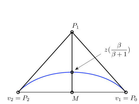
Figure 5: Conic as a rational Bézier curve.

Conversion to bivariate Bernstein-Bézier form

For the sake of computation of the system matrices in the finite element method we need to convert the conic from the parametric representation (31) into implicit form $q(x)=0$ where $q$ is a quadratic polynomial written in BB-form as

$$q=\sum_{i+j+k=2}\omega_{ijk}B_{ijk}^{2},\quad\omega_{ijk}\in\mathbb{R},$$

with respect to the triangle $T^{*}$ associated with a pie-shaped triangle $T\in\triangle_{P}$, see Figure 6. Let $v_{1}=P_{0}$ and $v_{2}=P_{2}$ be the boundary vertices of $T$, and let $v_{3}$ be its interior vertex. Since $q(v_{1})=q(v_{2})=0$, we have $\omega_{200}=\omega_{020}=0$, and arrive at

$$q=\omega_{110}B_{110}^{2}+\omega_{101}B_{101}^{2}+\omega_{011}B_{011}^{2}+\omega_{002}B_{002}^{2},$$ (32)

or, more explicitly,

$$q=2(\omega_{110}b_{1}b_{2}+\omega_{101}b_{1}b_{3}+\omega_{011}b_{2}b_{3})+\omega_{002}b_{3}^{2}.$$

\psfrag{c}{$\omega$}\includegraphics[width=245.26274pt]{BezierNetq.eps}

Figure 6: BB-coefficients of $q$ over a pie-shaped triangle.

To compute the yet unknown coefficients of $q$, we obtain three linear equations from the facts that the point $z=(1-s)M+s{P}_{1}$ lies on the conic, and the tangential directional derivatives of $q$ at $P_{i}$, $i=0,1$, vanish. Let $\alpha_{1},\alpha_{2},\alpha_{3}$ be the barycentric coordinates of the control point ${P}_{1}$ w.r.t. $T^{*}$. Then the barycentric coordinates of $z$ are $\tfrac{1-s}{2}+s\alpha_{1},\;\tfrac{1-s}{2}+s\alpha_{2},\;s\alpha_{3}$, so that $q(z)=0$ leads to the equation

$$(\tfrac{1-s}{2}+s\alpha_{1})(\tfrac{1-s}{2}+s\alpha_{2})\omega_{110}+s\alpha_{3}(\tfrac{1-s}{2}+s\alpha_{1})\omega_{101}+s\alpha_{3}(\tfrac{1-s}{2}+s\alpha_{2})\omega_{011}+\tfrac{1}{2}(s\alpha_{3})^{2}\omega_{002}=0.$$

It is easy to see that $(\alpha_{1}-1,\alpha_{2},\alpha_{3})$ and $(\alpha_{1},\alpha_{2}-1,\alpha_{3})$ are the directional coordinates of the vectors $P_{0}{P}_{1}$ and ${P}_{2}{P}_{1}$ in the terminology of [20, Section 2.6]. Since

$$\partial_{P_{0}{P}_{1}}q(v_{1})=\partial_{P_{2}{P}_{1}}q(v_{2})=0,$$

we obtain using [20, Theorem 2.12],

$$\alpha_{2}\omega_{110}+\alpha_{3}\omega_{101}=0\;\text{ and }\;\alpha_{1}\omega_{110}+\alpha_{3}\omega_{011}=0,$$

which leads to

$$\Big{(}\big{(}\tfrac{1-s}{2}\big{)}^{2}-s^{2}\alpha_{1}\alpha_{2}\Big{)}\omega_{110}=-\tfrac{1}{2}(s\alpha_{3})^{2}\omega_{002}.$$

We observe that $\alpha_{3}=0$ if and only if ${P}_{1}$ lies on the straight line $P_{0}{P}_{2}$, which means that $q$ is zero on this line. This implies that the conditions $\alpha_{3}=0$ and $\omega_{110}=0$ are equivalent to each other and never hold for triangles in $\triangle_{P}$ because their boundary edges are not straight. Since $0<s<1$, it follows that $\omega_{002}=0$ if and only if $\big{(}\tfrac{1-s}{2}\big{)}^{2}-s^{2}\alpha_{1}\alpha_{2}=0$, or using the parameter $\beta$ of (31), $4\beta^{2}\alpha_{1}\alpha_{2}=1$. Since $\omega_{002}=q(v_{3})\neq 0$ by our assumptions, we assume without loss of generality that $q(v_{3})=1$, which implies

$$4\beta^{2}\alpha_{1}\alpha_{2}\neq 1$$

and the following formulas for the coefficients of $q$ in (32),

$$\omega_{110}=-\alpha_{3}\mu,\quad\omega_{101}=\alpha_{2}\mu,\quad\omega_{011}=\alpha_{1}\mu,\quad\mu:=\frac{2\beta^{2}\alpha_{3}}{1-4\beta^{2}\alpha_{1}\alpha_{2}};\quad\omega_{002}=1.$$ (33)

Since $T$ is star-shaped w.r.t. $v_{3}$, we always have $\alpha_{1},\alpha_{2}>0$. Moreover, $\alpha_{3}>0\,(<0)$ if ${P}_{1}$ lies inside $T$ (outside $T$). We show that the condition that $q(x)$ is positive for all $x$ in $T$ except of the curved edge is satisfied if and only if $\mu>0$, that is

$$\frac{\alpha_{3}}{1-4\beta^{2}\alpha_{1}\alpha_{2}}>0.$$ (34)

Indeed, if $\alpha_{3}>0$, then $T$ is a proper part of $T^{*}$. Connect $v_{3}$ by a straight line with any point $z$ on the segment $[v_{1},v_{2}]$. Then the univariate quadratic polynomial obtained by restricting $q$ to this straight line is positive at $v_{3}$, negative at $z$ and zero at the point of the curved edge it crosses. Hence it cannot be zero at any other point of $T$. If $\alpha_{3}<0$, then $T$ contains $T^{*}$ and is convex. By [20, Theorem 3.6], $q$ is positive everywhere in $T^{*}$ except the vertices $v_{1},v_{2}$ if and only if the coefficients $\omega_{110},\omega_{101},\omega_{011}$ are all positive, which is equivalent to $\mu>0$. As a conic, the curve $q(x)=0$ cannot have another branch inside $T\setminus T^{*}$.

Multiplication by $q$ on a pie-shaped triangle

We now work out formulas for the BB-coefficients $a_{ijk}$ of $s|_{T}$ in terms of the BB-coefficients of $q$ and those of the polynomial $p$ such that $s|_{T}=qp$. The formulas (35) have already been used in the proof of Theorem 4.7, and they will again be needed in Section 5.2.

Let

$$q=\omega_{110}B_{110}^{2}+\omega_{101}B_{101}^{2}+\omega_{011}B_{011}^{2}+B_{002}^{2}$$

and

$$s|_{T}=q\sum_{i+j+k=d-1}c_{ijk}B^{d-1}_{ijk}=\sum_{i+j+k=d+1}a_{ijk}B^{d+1}_{ijk}.$$

Since

$$qB^{d-1}_{ijk}=\; 2\tfrac{(i+1)(j+1)}{d(d+1)}\omega_{110}B^{d+1}_{i+1,j+1,k}+2\tfrac{(i+1)(k+1)}{d(d+1)}\omega_{101}B^{d+1}_{i+1,j,k+1}$$

$$+2\tfrac{(j+1)(k+1)}{d(d+1)}\omega_{011}B^{d+1}_{i,j+1,k+1}+\tfrac{(k+1)(k+2)}{d(d+1)}B^{d+1}_{i,j,k+2},$$

we get the following formula for the BB-coefficients of $s|_{T}$,

$$a_{ijk}=\tfrac{2ij\,\omega_{110}}{d(d+1)}c_{i-1,j-1,k}+\tfrac{2ik\,\omega_{101}}{d(d+1)}c_{i-1,j,k-1}+\tfrac{2jk\,\omega_{011}}{d(d+1)}c_{i,j-1,k-1}+\tfrac{(k-1)k}{d(d+1)}c_{i,j,k-2},$$ (35)

where $c_{r,s,t}:=0$ if at least one of the indices $r,s,t$ is negative.

5.2 Assembly of the finite element linear system

To compute the solution $\tilde{u}$ of (18) we follow the standard Galerkin scheme and expand $\tilde{u}$ as linear combination of the basis functions $s_{\xi}$, $\xi\in M_{0}$, of Section 4.3,

$$\tilde{u}=\sum_{\xi\in M_{0}}c_{\xi}s_{\xi},\quad c_{\xi}\in\mathbb{R}.$$

Then (18) is equivalent to the square linear system

$$\sum_{\xi\in M_{0}}c_{\xi}a(s_{\xi},s_{\zeta})=(f,s_{\zeta})\;\text{ for all }\zeta\in M_{0}$$

with a positive definite system matrix $[a(s_{\xi},s_{\zeta})]_{\xi,\zeta\in M_{0}}$. For the elliptic equations of second order we have

$$a(u,v)=\int_{\Omega}(\nabla u\cdot A\nabla v+v{\bf b}\cdot\nabla u+cuv)dx,$$

where $A$ is a matrix, ${\bf b}$ a vector and $c$ a scalar, each of them in general depending on $x$. Hence, assembling the matrix requires the computation of the following system matrices: the stiffness matrix $\mathcal{S}$, the convective matrix $\mathcal{B}$ and the mass matrix $\mathcal{M}$, whose entries are given by

$$\mathcal{S}_{\xi\zeta}=\int_{\Omega}\nabla s_{\xi}\cdot A\nabla s_{\zeta}dx,\quad\mathcal{B}_{\xi\zeta}=\int_{\Omega}s_{\zeta}{\bf b}\cdot\nabla s_{\xi}dx,\quad\mathcal{M}_{\xi\zeta}=\int_{\Omega}cs_{\xi}s_{\zeta}dx,\quad\xi,\zeta\in M_{0},$$

while the right hand side of the system requires the computation of the load vector $\mathcal{L}$ with entries

$$\mathcal{L}_{\xi}=\int_{\Omega}fs_{\xi}dx,\quad\xi\in M_{0}.$$

By integrating over all triangles $T\in\triangle$ we can reduce the assembly problem to the computation of the element level system matrices and load vector

$$\hat{\mathcal{S}}_{T}=\Big{[}\int_{T}\nabla B^{d+i}_{\xi}\cdot A\nabla B^{d+i}_{\zeta}dx\Big{]}_{\xi,\zeta\in D_{d+i,T^{*}}},\;\hat{\mathcal{B}}_{T}=\Big{[}\int_{T}B^{d+i}_{\xi}{\bf b}\cdot\nabla B^{d+i}_{\zeta}dx\Big{]}_{\xi,\zeta\in D_{d+i,T^{*}}},$$

$$\hat{\mathcal{M}}_{T}=\Big{[}\int_{T}cB^{d+i}_{\xi}B^{d+i}_{\zeta}dx\Big{]}_{\xi,\zeta\in D_{d+i,T^{*}}},\;\hat{\mathcal{L}}_{T}=\Big{[}\int_{T}fB^{d+i}_{\xi}dx\Big{]}_{\xi\in D_{d+i,T^{*}}},$$

where $i=0$ if $T\in\triangle_{0}$, $i=1$ if $T\in\triangle_{P}\cup\triangle_{B}$, and $T^{*}$ is defined as above for $T\in\triangle_{P}$ and simply as $T^{*}=T$ otherwise. Indeed, it is easy to see that

$$\mathcal{S}=\mathcal{T}^{t}\hat{\mathcal{S}}\mathcal{T},\;\mathcal{B}=\mathcal{T}^{t}\hat{\mathcal{B}}\mathcal{T},\;\mathcal{M}=\mathcal{T}^{t}\hat{\mathcal{M}}\mathcal{T},\;\mathcal{L}=\mathcal{T}^{t}\hat{\mathcal{L}},$$ (36)

where

$$\hat{\mathcal{S}} :=\operatorname{diag}(\hat{\mathcal{S}}_{T},T\in\triangle),\quad\hat{\mathcal{B}}:=\operatorname{diag}(\hat{\mathcal{B}}_{T},T\in\triangle),$$

$$\hat{\mathcal{M}} :=\operatorname{diag}(\hat{\mathcal{M}}_{T},T\in\triangle),\quad\hat{\mathcal{L}}:=[\hat{\mathcal{L}}_{T}^{t},T\in\triangle],$$

and $\mathcal{T}$ is the transformation matrix whose columns correspond to the basis functions $s_{\xi}$, $\xi\in M_{0}$, and consist of the BB-coefficients of $s_{\xi}|_{T}$ on all triangles $T\in\triangle$, and $\mathcal{T}^{t}$ is the transpose of $\mathcal{T}$.

The structure of the transformation matrix is rather simple. Let $\tau_{\xi}$ denote the column of $\mathcal{T}$ corresponding to $\xi\in M_{0}$, such that $\mathcal{T}=[\tau_{\xi}]_{\xi\in M_{0}}$. If $\xi\in D_{d,\triangle_{0}}$ and $\xi$ is not contained in any pie-shaped or buffer triangle, then the only non-zero entries of $\tau_{\xi}$ are the ones at every row corresponding to $\xi\in D_{d,T}$ for some $T\in\triangle_{0}$. Similarly, if $\xi\in D^{0}_{d+1,T}$ for some $T\in\triangle_{B}$, then $\tau_{\xi}$ also consists of ones and zeros, with ones at all rows corresponding to the same $\xi$ in one or more triangles of $\triangle_{B}$. If $\xi=\xi_{ijk}\in D^{*}_{d-1,T}$ for some $T\in\triangle_{P}$, then four entries of $\tau_{\xi}$ will be non-zero in rows corresponding to $\xi_{i+1,j+1,k}$, $\xi_{i+1,j,k+1}$, $\xi_{i,j+1,k+1}$, $\xi_{i,j,k+2}$ in $D_{d+1,T^{*}}$. These entries can be determined from the equation (35) as

$$\tfrac{2(i+1)(j+1)\,\omega_{110}}{d(d+1)},\quad\tfrac{2(i+1)(k+1)\,\omega_{101}}{d(d+1)},\quad\tfrac{2(j+1)(k+1)\,\omega_{011}}{d(d+1)},\quad\tfrac{(k+1)(k+2)}{d(d+1)},$$

respectively. If $i=0$ and $j\neq 0$, then the domain points $\xi_{i,j+1,k+1}=\xi_{0,j+1,k+1}$ and $\xi_{i,j,k+2}=\xi_{0,j,k+2}$ lie on an edge of $T$ shared with a triangle $T^{\prime}$ in $\triangle_{P}\cup\triangle_{B}$, and hence the two entries of $\tau_{\xi}$ corresponding to these points in $T^{\prime}$ will be filled with the numbers $\tfrac{2(j+1)(k+1)\,\omega_{011}}{d(d+1)}$, $\tfrac{(k+1)(k+2)}{d(d+1)}$, respectively. Similarly, there are two additional nonzero entries in the case $i\neq 0$, $j=0$. If $i=j=0$, then $k=d-1$ and $\xi_{i,j,k+2}=\xi_{0,0,d+1}$ is the interior vertex $v$ of $T$. It is clear from the above that the nonzero entries of $\tau_{v}$ are: (a) the ones at all rows corresponding to $v$ in any types of triangles containing this vertex, (b) the numbers $\tfrac{2\,\omega_{110}}{d(d+1)}$, $\tfrac{2\,\omega_{101}}{d+1}$, $\tfrac{2\,\omega_{011}}{d+1}$ placed in the rows corresponding to $\xi_{1,1,d-1}$, $\xi_{1,0,d}$, $\xi_{0,1,d}$, respectively, in all pie-shaped triangles attached to $v$ (where $\omega_{110},\omega_{101},\omega_{011}$ depend on the pie-shaped triangle), and (c) the number $\tfrac{2\,\omega_{101}}{d+1}$ or $\tfrac{2\,\omega_{011}}{d+1}$ in the row corresponding to $\xi_{1,0,d}$ or $\xi_{0,1,d}$ if it belong to a buffer triangle attached to the respective pie-shaped triangle. Finally, assume that $\xi\in D_{d,\triangle_{0}}\cap T$ for a buffer triangle $T$, but $\xi$ is not a vertex of any pie-shaped triangle. Then $\xi=\xi_{ijk}$ for some $i,j,k$ with $i+j+k=d$, as element of $D_{d,T}$. (Note that at least one of the indices $i,j,k$ is zero because $\xi$ lies on an edge of $T$.) Then by using the well known degree raising formulas [20, Theorem 2.39], we see that the non-zero entries of $\tau_{\xi}$ are, in addition to ones in the rows corresponding to $\xi$ in all triangles of $\triangle_{0}$ containing $\xi$, the numbers $\tfrac{i+1}{d+1}$, $\tfrac{j+1}{d+1}$, $\tfrac{k+1}{d+1}$ in the rows corresponding to $\xi_{i+1,j,k}$, $\xi_{i,j+1,k}$ and $\xi_{i,j,k+1}$ as elements of $D_{d+1,T}$, for each buffer triangle $T$ containing $\xi$.

Note that the global-local transformation (36) can be performed without explicit evaluation and storage of the transformation matrix $\mathcal{T}$. Instead, suitable routines for the matrix-vector products $\mathcal{T}x$ and $\mathcal{T}^{t}x$ need to be implemented, and this can be done efficiently with $\mathcal{O}(d^{2})$ computation cost per triangle $T\in\triangle$, similar to the algorithms in [4, Section 8.1].

As shown in [2], the element level system matrices can be computed with optimal $\mathcal{O}(1)$ cost per entry on the non-curved triangles. Indeed, the product formula for Bernstein polynomials

$$B_{ijk}^{d}B_{rst}^{q}=\frac{{{i+r}\choose{i}}{{j+s}\choose{j}}{{k+t}\choose{k}}}{{{d+q}\choose{d}}}B_{i+r,j+s,k+t}^{d+q}$$

helps to reduce this task to the computation of the Bernstein-Bézier (BB-) moments

$$\mu^{T,m}_{\xi}(g):=\int_{T}g(x)B^{m}_{\xi}(x)\,dx,\qquad\xi\in D_{m,T},$$

where $g$ is one of the functions $A,{\bf b},c$ and $m$ is a number between $2d-2$ and $2d+2$. The components of the load vector $\hat{\mathcal{L}}_{T}$ are just the moments of $f$ of degree $m=d$ or $d+1$. Using [2, Algorithm 3], the moment vector $\mu^{T,m}(g):=[\mu^{T,m}_{\xi}(g)]_{\xi\in D_{m,T}}$ can be evaluated with $\mathcal{O}(m^{3})$ floating point operations with the help of an $\mathcal{O}(m^{2})$-point Stroud quadrature, which delivers sufficient accuracy for the finite element approximation.

If $T\in\triangle_{P}$, then the same approach can be used, where we only need to figure out how to compute the BB-moments.

5.3 BB-moments on curved triangles

We show that for any pie-shaped triangle $T\in\triangle_{P}$ the moment vector $\mu^{T,m}(f)$ can be computed with $\mathcal{O}(q^{2}m)$ operations using a quadrature rule with $q^{2}$ centers, which is exact for all $f\in\mathbb{P}_{2q-m-1}$, $q>m/2$. This means that $q=\mathcal{O}(d)$ points guarantee sufficient accuracy, and hence the element level system matrices are computed on pie-shaped triangles also with optimal computation cost $\mathcal{O}(1)$ per entry [2].

As before let $v_{1},v_{2}$ be the boundary vertices of $T$, and $v_{3}$ its interior vertex. We consider a version of Duffy transformation $\Phi$ [2, Section 3.1] that maps any point $(t_{1},t_{2})\in\mathbb{R}^{2}$ into $\Phi(t_{1},t_{2})=b_{1}v_{1}+b_{2}v_{2}+b_{3}v_{3}$, where

$$b_{1}=(1-t_{1})t_{2},\quad b_{2}=t_{1}t_{2},\quad b_{3}=1-t_{2}.$$ (37)

It is easily seen that the straight triangle $T^{*}$ with vertices $v_{1},v_{2},v_{3}$ is the image of the unit square, that is $T^{*}=\Phi([0,1]^{2})$, with $v_{1}=\Phi(0,1)$, $v_{2}=\Phi(1,1)$, $v_{3}=\Phi(1,0)=\Phi(0,0)$. For any constant $\tau$ the image of the straight line $t_{1}=\tau$ is the straight line going through $v_{3}$ and the point $(1-\tau)v_{1}+\tau v_{2}$ lying on the line through $v_{1},v_{2}$. The pie-shaped triangle $T$ is the image of

$$\hat{T}:=\{(t_{1},t_{2})\in\mathbb{R}^{2}:0\leq t_{1}\leq 1,\;0\leq t_{2}\leq\phi(t_{1})\},$$

where $\phi$ is a continuous function which is well defined because $T$ is star-shaped with respect to $v_{3}$. Assuming that the curved edge of $T$ is given by the equation $q(x)=0$, with $q$ defined by (32), $\phi(\tau)$ is easy to compute for any $0\leq\tau\leq 1$ as the first positive root of the univariate quadratic polynomial

$$\tilde{q}(t) =q(v_{3}+t((1-\tau)v_{1}+\tau v_{2}-v_{3}))$$

$$=\omega_{002}B^{2}_{0}(t)+\big{(}\omega_{101}(1-\tau)+\omega_{011}\tau\big{)}B^{2}_{1}(t)+2\omega_{110}(1-\tau)\tau B^{2}_{2}(t),$$

where we use quadratic Bernstein polynomials $B^{2}_{i}$ as in (31).

Since the Jacobian of $\Phi$ is $2|T^{*}|t_{2}$, where $|M|$ denotes the area of a set $M\subset\mathbb{R}^{2}$, we can compute any integral over $T$ as

$$\int_{T}f(x)\,dx=2|T^{*}|\int_{0}^{1}dt_{1}\int_{0}^{\phi(t_{1})}f(\Phi(t_{1},t_{2}))t_{2}\,dt_{2}.$$

By applying Gauss-Legendre, respectively Gauss-Jacobi quadrature with $q$ points,

$$\int_{0}^{1}g(s)\,ds\approx\sum_{j=1}^{q}w_{j}g(\xi_{j}),\qquad\int_{0}^{1}sg(s)\,ds\approx\sum_{j=1}^{q}\tilde{w}_{j}g(\tilde{\xi}_{j}),$$

to the integrals in $t_{1}$, respectively $t_{2}$, we obtain a positive quadrature rule with $q^{2}$ centers

$$\int_{T}f(x)\,dx\approx 2|T^{*}|\sum_{\mu=1}^{q}w_{\mu}\phi^{2}(\xi_{\mu})\sum_{\nu=1}^{q}\tilde{w}_{\nu}f(\xi_{\nu\mu}),\quad\text{with }\;\xi_{\nu\mu}:=\Phi(\xi_{\mu},\phi(\xi_{\mu})\tilde{\xi}_{\nu}),$$ (38)

which is exact whenever $f\in\mathbb{P}_{2q-1}$ since $f(\Phi(t_{1},t_{2}))$ is a univariate polynomial of degree $2q-1$ in each of $t_{1},t_{2}$ in that case.

Similar to [2, Lemma 1] the bivariate Bernstein polynomials with respect to $T^{*}$ can be factorized as

$$B^{m}_{ijk}(x)=B^{m-k}_{j}(t_{1})B^{m}_{k}(t_{2}),\quad x=\Phi(t_{1},t_{2}),$$

where $B^{n}_{\nu}(t)={n\choose\nu}t^{\nu}(1-t)^{n-\nu}$, $0\leq\nu\leq n$, are the univariate Bernstein polynomials. Hence, by using (38) we obtain the following approximation of the moments for all $i+j+k=m$,

$$\mu^{T,m}_{ijk}(f)\approx 2|T^{*}|\sum_{\mu=1}^{q}w_{\mu}\phi^{2}(\xi_{\mu})B^{m-k}_{j}(\xi_{\mu})\sum_{\nu=1}^{q}\tilde{w}_{\nu}B^{m}_{k}(\phi(\xi_{\mu})\tilde{\xi}_{\nu})f(\xi_{\nu\mu}).$$ (39)

Since $B^{m}_{ijk}$ is a polynomial of degree $m$ in $t_{2}$ and at most $m$ in $t_{1}$, the formula (39) is exact for all $f\in\mathbb{P}_{2q-m-1}$ as long as $q>m/2$, and its structure allows evaluation by sum factorization as in [2, Section 3.3]. That is, first the sums

$$\sigma_{\mu,k}=\sum_{\nu=1}^{q}\tilde{w}_{\nu}B^{m}_{k}(\phi(\xi_{\mu})\tilde{\xi}_{\nu})f(\xi_{\nu\mu})$$

are computed for all $\mu=1,\ldots,q$ and $k=0,\ldots,m$ with $\mathcal{O}(q^{2}m)$ cost, and then the numbers

$$2|T^{*}|\sum_{\mu=1}^{q}w_{\mu}\phi^{2}(\xi_{\mu})B^{m-k}_{j}(\xi_{\mu})\sigma_{\mu,k},\quad k=0,\ldots,m,\;j=0,\ldots,m-k,$$

give the moments $\mu^{T,m}_{ijk}(f)$, $i=m-j-k$, with the cost of $\mathcal{O}(qm^{2})$.

6 Numerical experiments

To test the numerical performance of our method we implemented it in MATLAB and present in this section three examples including the membrane eigenvalue problem and Poisson problem on different domains with curved boundaries. We consider both $h$- and $p$-refinements and compare our results to the state-of-the-art software COMSOL Multiphysics. We use version 4.2a of COMSOL which provides the options to employ the standard isoparametric elements of degree up to 5 on curved domains in 2D. While the domains in Examples 1 and 2 are smooth (an ellipse and a circle), we consider a $C^{0}$ domain bounded by linear and conic pieces in Example 3. The numerics confirm in particular the theoretical rate of convergence given in Theorem 3.4. Note that for simplicity we used an easier implementation which does not achieve optimal cost assembly described in Section 5. (Further details can be found in [21].)

Example 1: Poisson problem on an ellipse

Let $\Omega$ be the domain in $\mathbb{R}^{2}$ bounded by the ellipse $x_{1}^{2}+6.25x_{2}^{2}=1$. Consider the boundary value problem

$$\Delta u=f\mbox{ in }\Omega,\quad u=0\mbox{ on }\partial\Omega,$$ (40)

where $f$ is chosen such that the exact solution of the problem is $u=e^{0.5(x_{1}^{2}+6.25x_{2}^{2})}-e^{0.5}$.

To ensure a fair comparison of the numerical results with COMSOL, we use the initial triangulation shown in Figure 7 generated by COMSOL. We obtain a sequence of triangulations by uniform refinement whereby each triangle is subdivided into four subtriangles by joining the midpoints of all edges. For a pie-shaped triangle we take the midpoint of the curved boundary edge, see Figure 8.

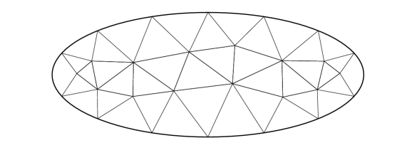
Figure 7: Example 1: Initial triangulation.

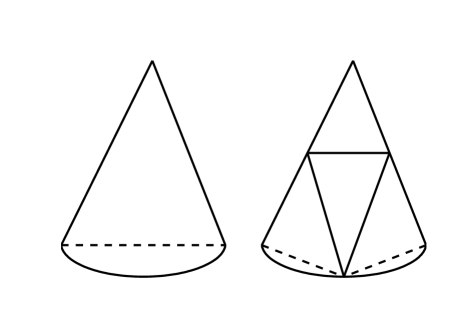
Figure 8: Refinement of a pie-shaped triangle.

Error plots for $\|u-u_{N}\|_{L_{2}(\Omega)}$ and $\|u-u_{N}\|_{H^{1}(\Omega)}$ as functions of the number of degrees of freedom $N=\dim S_{d,0}(\triangle)$ are depicted in Figures 9 and 10, respectively, for $d=2,3,4,5$, where $u_{N}\in S_{d,0}(\triangle)$ is the approximate solution to the problem, and different points on the curves correspond to subsequent refinements of the triangulation. The results show that both methods behave similarly for all different orders and confirm the theoretical estimates of Theorem 3.4. Furthermore, Figure 11 demonstrates the expected exponential decay of errors of our method in an experiment of a “$p$-refinement” type [6], where the triangulation is fixed (as obtained by two subsequent uniform refinements of the initial triangulation), and the degree $d$ is increased instead, increasing this way the number of degrees of freedom.

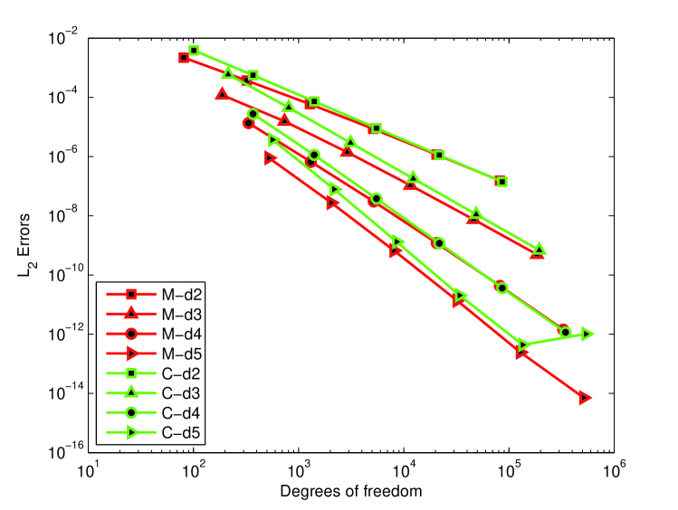
Figure 9: $L_{2}$ errors in Example 1 using our method (red) and COMSOL (green). The curves indicated by d2, d3, d4, d5 correspond to the degrees $d=2,\ldots,5$.

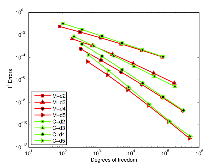
Figure 10: $H^{1}$ errors in Example 1 using our method (red) and COMSOL (green).

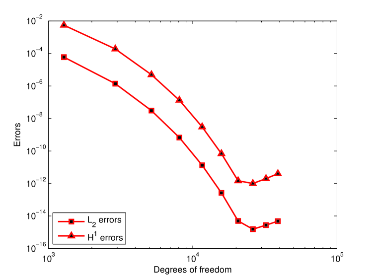
Figure 11: $L_{2}$ and $H^{1}$ errors in Example 1 using $p$-refinement.

Example 2: Circular membrane eigenvalue problem

The free vibrations of a homogeneous membrane are governed by the equation

$$\Delta u+\lambda u=0,\quad x\in\Omega.$$ (41)

If the membrane is fixed along its boundary then the boundary condition is

$$u=0,\quad x\in\partial\Omega,$$ (42)

which comprises a problem of finding eigenvalues and eigenfunctions of the Laplacian under homogeneous Dirichlet boundary conditions.

We choose $\Omega\subset\mathbb{R}^{2}$ to be a unit disk and approximate 15 smallest eigenvalues for the circular membrane. The exact solution to this problem is known [19], with the eigenvalues given by

$$\lambda_{m,n}=(j_{m,n})^{2},\quad m=0,1,\ldots,\quad n=1,2,\ldots,$$

where $j_{m,n}$ is the $n$-th root of the $m$-th Bessel function $J_{m}$ of the first kind.

The weak variational formulation corresponding to (41) and (42), for $\lambda\in\mathbb{R}$ and $u\neq 0$, is

$$\mbox{ Find }\,u\in H^{1}_{0}(\Omega),\;\int_{\Omega}\nabla u\cdot\nabla v=\lambda\int_{\Omega}uv,\;\hbox{$\forall$ $v\in H^{1}_{0}(\Omega)$.}$$ (43)

We discretize this problem in the space $S_{d,0}(\triangle)$ for a suitable triangulation of $\Omega$: Find $\tilde{u}\in S_{d,0}(\triangle)$, $\tilde{u}\neq 0$, such that

$$\int_{\Omega}\nabla\tilde{u}\cdot\nabla\tilde{v}=\lambda\int_{\Omega}\tilde{u}\tilde{v},\quad\hbox{$\forall\tilde{v}\in S_{d,0}(\triangle)$.}$$ (44)

Hence if $\left\{s_{1},\ldots,s_{N}\right\}$ is a for $S_{d,0}(\triangle)$ according to Theorem 4.7, then (44) boils down to the matrix equation of the form

$$\mathcal{S}=\lambda\mathcal{M},$$

where $\mathcal{S}$ and $\mathcal{M}$ are the stiffness and mass matrices. We solve this generalized matrix eigenvalue problem using MATLAB’s built-in command eig.

We follow the same procedure to get a sequence of meshes as in Example 1, starting with the initial mesh shown in Figure 12 imported from COMSOL. Note that this triangulation does not satisfy (5).

Figure 12: Initial triangulation of the unit circle for Example 2.

In Figures 13–16 we plot absolute errors for approximating various eigenvalues using our implementation and using COMSOL for degree $d=3$ and $d=5$. It can be seen that, comparing to COMSOL, our method approximates the first two eigenvalues significantly better. For the 8th and 15th eigenvalues the results are comparable for $d=3$ but for the higher degree $d=5$ the accuracy achieved using our method is again better. Figure 17 depicts the errors of our method for the first 15 eigenvalues for degree $d=9$. It is easy to check that the slopes of the curves in Figures 13–17 are consistent with the expected convergence rate $h^{2d}$ which follows from Theorem 3.3 in view of [5, Theorem 3.1].

We have also tested the $p$-refinement for this problem on the initial triangulation shown in Figure 12. We plot the absolute errors for the 1st, 7th and 15th eigenvalues in Figure 18. For comparison, the figure also includes the errors obtained with COMSOL up the highest degree 5 it allows. The rate of convergence is exponential in this case as expected.

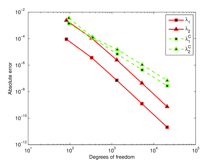
Figure 13: Example 2: Absolute errors for 1st and 2nd eigenvalues by our method $(\lambda_{1},\lambda_{2})$ and by COMSOL ($\lambda^{C}_{1}$,$\lambda^{C}_{2}$) for $d=3$.

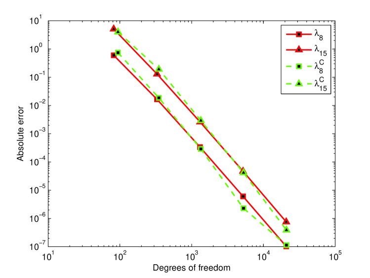
Figure 14: Example 2: Absolute errors for 8th and 15th eigenvalues for $d=3$ ($\lambda_{8},\lambda_{15}$: our method, $\lambda^{C}_{8},\lambda^{C}_{15}$: COMSOL).

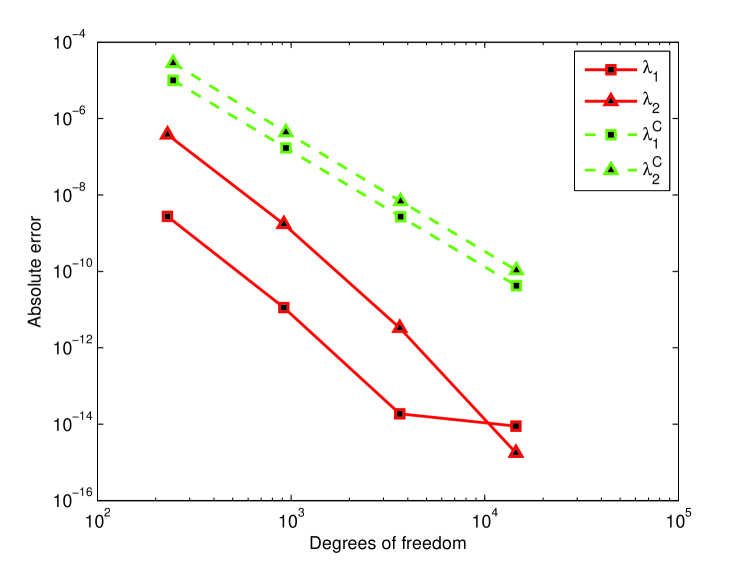
Figure 15: Example 2: Absolute errors for 1st and 2nd eigenvalues for $d=5$ ($\lambda_{1},\lambda_{2}$: our method, $\lambda^{C}_{1},\lambda^{C}_{2}$: COMSOL).

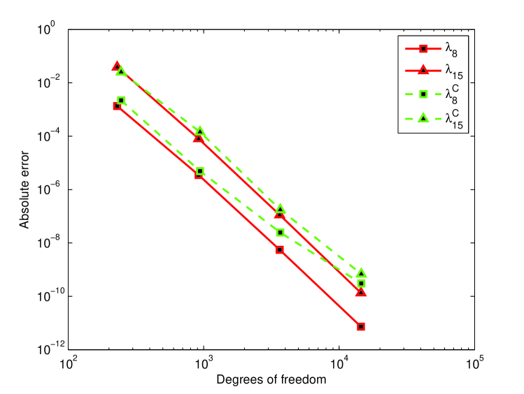
Figure 16: Example 2: Absolute errors for 8th and 15th eigenvalues for $d=5$ ($\lambda_{8},\lambda_{15}$: our method, $\lambda^{C}_{8},\lambda^{C}_{15}$: COMSOL).

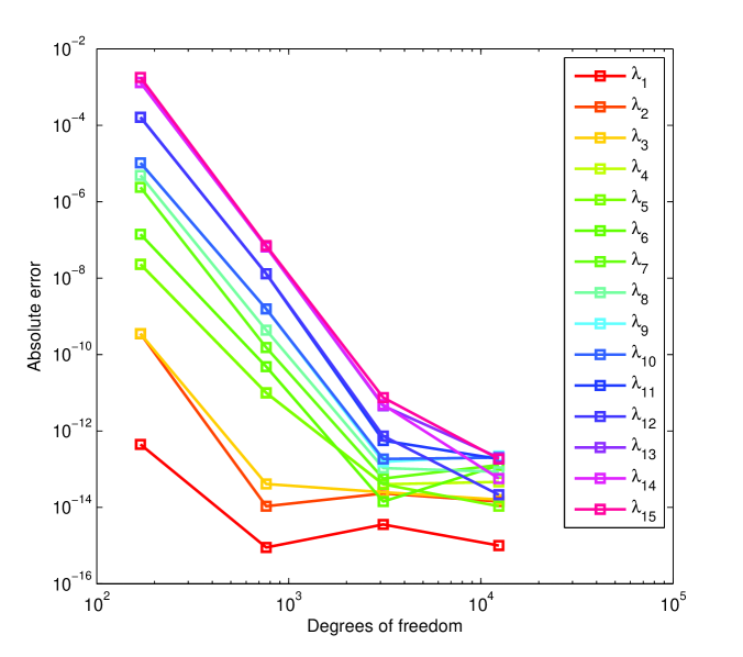
Figure 17: Example 2: Absolute errors for the first 15 eigenvalues using our method for $d=9$.

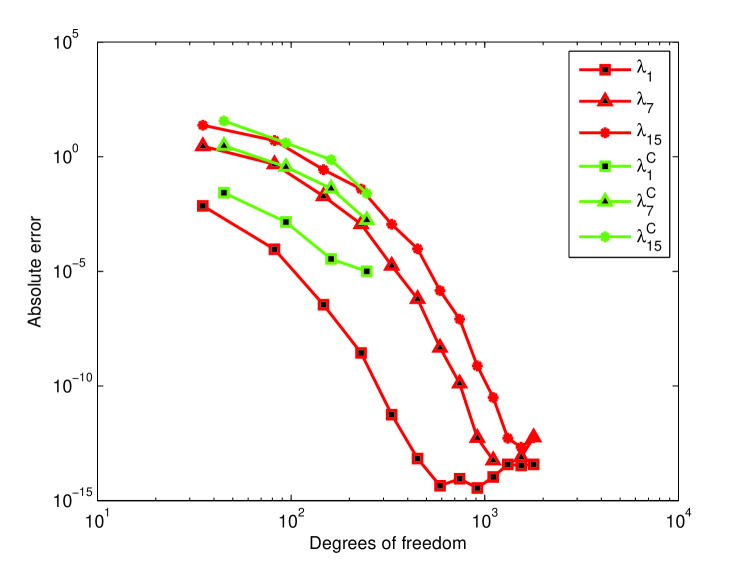
Figure 18: Example 2: Absolute errors for the 1st, 7th and 15th eigenvalues using $p$-refinement over initial triangulation shown in Figure 12 ($\lambda_{1},\lambda_{7},\lambda_{15}$: our method, $\lambda^{C}_{1},\lambda^{C}_{7},\lambda^{C}_{15}$: COMSOL).

Example 3: Poisson problem on a $C^{0}$ piecewise conic domain

Here we consider a domain $\Omega$ with $C^{0}$ boundary bounded by linear and quadratic boundary segments. The boundary is defined by two straight lines $x_{2}=\pm 2$ and two parabolas $x_{1}=\pm(x_{2}^{2}-6)$. We consider the Poisson problem (40), where $f$ is chosen such that the exact solution is $u=(x_{2}^{2}-4)(x_{1}^{2}-(x_{2}^{2}-6)^{2})/100$.

Similar to Example 1 we consider elements of degrees $d=2,3,4,5$ and compare our results with COMSOL. Figures 19 and 20 depict the $L_{2}$ and $H^{1}$ errors for both methods. Again the numbers show the robust behavior of our method for different degrees while confirming the error bounds of Theorem 3.4. We do not consider the $p$-refinement for this example because the solution is a polynomial of degree 6 and hence lies in the approximation space $S_{d,0}(\triangle)$ for all $d\geq 6$.

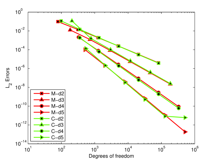
Figure 19: $L_{2}$-errors in Example 3 using our method and COMSOL.

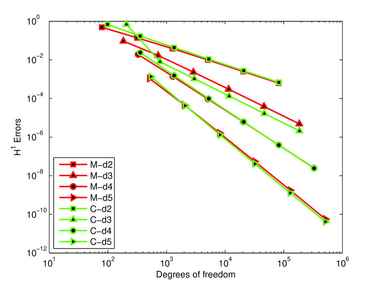
Figure 20: $H^{1}$-errors in Example 3 using our method and COMSOL.

References

- [1]
- [2] M. Ainsworth, G. Andriamaro and O. Davydov, Bernstein-Bézier finite elements of arbitrary order and optimal assembly procedures, SIAM J. Sci. Comp., 33 (2011), 3087–3109.
- [3] M. Ainsworth, G. Andriamaro and O. Davydov, A Bernstein-Bézier basis for arbitrary order Raviart-Thomas finite elements, Constr. Approx. 41 (2015), 1–22.
- [4] M. Ainsworth, L. L. Schumaker and O. Davydov, Bernstein-Bézier finite elements on tetrahedral-hexahedral-pyramidal partitions, preprint, 40 pages.
- [5] I. Babuška, and J. Osborn, Estimates for the errors in eigenvalue and eigenvector approximation by Galerkin methods, with particular attention to the case of multiple eigenvalues, SIAM J. Numer. Anal., 24(6) 1987, 1249–1276.
- [6] I. Babuska, M. Suri, The p- and h-p versions of the finite element method, basic principles and properties, SIAM Review, 36(4), pp. 578-632, (1994).
- [7] J. Bloomenthal et al, Introduction to Implicit Surfaces, Morgan-Kaufmann Publishers Inc., San Francisco, 1997.
- [8] K. Böhmer, On finite element methods for fully nonlinear elliptic equations of second order, SIAM J. Numer. Anal., 46 (3) (2008), 1212–1249.
- [9] S. C. Brenner, and L.R. Scott, The Mathematical Theory of Finite Element Methods, Springer, New York, 1994.
- [10] A. Buffa, D. Cho, and G. Sangalli, Linear independence of the T-spline blending functions associated with some particular T-meshes. Computer Methods in Applied Mechanics and Engineering 199 (2010), 1437–1445.
- [11] O. Davydov, Stable local bases for multivariate spline spaces, J. Approx. Theory 111 (2001), 267–297.
- [12] O. Davydov and A. Saeed, Stable splitting of bivariate spline spaces by Bernstein-Bézier methods, in “Curves and Surfaces - 7th International Conference, Avignon, France, June 24-30, 2010” (J.-D. Boissonnat et al, Eds.), LNCS 6920, Springer-Verlag, 2012, pp. 220–235.
- [13] O. Davydov and A. Saeed, Numerical solution of fully nonlinear elliptic equations by Böhmer’s method, J. Comput. Appl. Math., 254 (2013), 43–54.
- [14] O. Davydov and A. Saeed, piecewise polynomial splines on curved domains and numerical solution of fully nonlinear elliptic equations, in preparation.
- [15] G. Farin, Curves and surfaces for CAGD: a practical guide, Fifth edition, Morgan Kaufmann Publishers Inc., San Francisco, CA, USA, 2002.
- [16] J. Hoschek and D. Lasser, Fundamentals of Computer Aided Geometric Design, A. K. Peters Ltd, Wellesley, MA, 1993.
- [17] K. Höllig, U. Reif and J. Wipper, Weighted extended B-spline approximation of Dirichlet problem, SIAM J. Numer. Anal., 39 (2) (2001), 442-462.
- [18] T. J. R. Hughes, J. A. Cottrel, Y. Bazilevs, Isogeometric analysis: CAD, finite elements, NURBS, exact geometry and mesh refinement, Comput. Methods Appl. Mech. Engrg., 194(2005) 4135-4195.
- [19] J. R. Kuttler, V. G. Sigillito, Eigenvalues of the Laplacian in Two Dimensions, SIAM, 26(2) (1984), 163–193.
- [20] M. J. Lai and L. L. Schumaker, Spline Functions on Triangulations, Cambridge University Press, 2007.
- [21] A. Saeed, Bivariate Piecewise Polynomials on Curved Domains, with Applications to Fully Nonlinear PDE’s, PhD thesis, University of Strathclyde, Glasgow, 2012.
- [22] L. L. Schumaker, Spline Functions: Computational Methods, SIAM (Philadelphia), 2015.
- [23] Ch. Schwab, - and -Finite Element Methods, Clarendon Press, Oxford, 1998.