Graphs in the 3-sphere with maximum symmetry

Abstract

We consider the orientation-preserving actions of finite groups $G$ on pairs $(S^{3},\Gamma)$, where $\Gamma$ is a connected graph of genus $g>1$, embedded in $S^{3}$. For each $g$ we give the maximum order $m_{g}$ of such $G$ acting on $(S^{3},\Gamma)$ for all such $\Gamma\subset S^{3}$. Indeed we will classify all graphs $\Gamma\subset S^{3}$ which realize these $m_{g}$ in different levels: as abstract graphs and as spatial graphs, as well as their group actions.

Such maximum orders without the condition “orientation-preserving” are also addressed.

Keywords symmetry of graph, symmetry of 3-sphere, extendable action

MSC 57M60, 57M15, 05E18

1 Introduction

We will study smooth, faithful actions of finite groups $G$ on pairs $(S^{3},\Gamma)$, where $\Gamma$ denotes a finite connected graph with an embedding $e:\Gamma\to S^{3}$. We also say that such a $G$-action on $\Gamma$ is extendable (w.r.t. $e$). Let $g(\Gamma)$ denote the genus of $\Gamma$, defined as the rank of its fundamental group (which is a free group). We will always assume that $g>1$ in the present paper.

Except in Section 5 we will only consider orientation-preserving finite group actions on $S^{3}$. Referring to the recent geometrization of finite group actions on $S^{3}$ (see [Pe]), we will consider only orthogonal actions of finite groups on $S^{3}$, i.e., finite subgroups $G$ of the orthogonal group $SO(4)$.

Let $m_{g}$ denote the maximum order of such a group $G$ acting on a pair $(S^{3},\Gamma)$, for all embeddings of finite graphs $\Gamma$ of a fixed genus $g$ into $S^{3}$. In this paper we will determine $m_{g}$ and classify all finite graphs $\Gamma$ which realize the maximum order $m_{g}$.

A similar question for the pair $(S^{3},\Sigma_{g})$, where $\Sigma_{g}$ is the closed orientable surface of genus $g$, was studied in [WWZZ]. The corresponding maximum order $OE_{g}$ of finite groups acting on $(S^{3},\Sigma_{g})$ for all possible embeddings $\Sigma_{g}\subset S^{3}$ was obtained in that paper.

Let $V_{g}$ denote the handlebody of genus $g$. Each graph $\Gamma\subset S^{3}$ of genus $g$ has a regular neighborhood which is homeomorphic to $V_{g}$. Call $\Gamma$ unknotted if the complement of its regular neighborhood is also a handlebody, and otherwise knotted.

Our first result is from a simple but significant observation, which claims $m_{g}=OE_{g}$, and can be considered as a version of [WWZZ, Theorem 1.1].

Theorem 1.1.

For each $g>1$, $m_{g}=OE_{g}$, therefore $m_{g}$ are given in the following table.

$m_{g}$	$g$
$12(g-1)$	$2,3,4,5,6,9,11,17,25,97,121,241,601$
$8(g-1)$	$7,49,73$
$20(g-1)/3$	$16,19,361$
$6(g-1)$	$21,481$
$24(g-1)/5$	$41$
$30(g-1)/7$	$29,841,1681$
$4(\sqrt{g}+1)^{2}$	$g=k^{2},k\neq 3,5,7,11,19,41$
$4(g+1)$	remaining numbers

Moreover $m_{g}$ is realized by unknotted graphs for all $g$ except $g=21,481$.

The difference between graph case and surface case is that, given a fixed $g$, there is a unique closed orientable surface of genus $g$, but there are infinitely many graphs of genus $g$. We will consider only minimal graphs, i.e, the graphs without free edges and without extra vertices: an edge is called free if one of its vertices has degree one; a vertex is extra if it has degree two and its stable subgroup (stablizer in $G$) equals the stable subgroup of each adjacent edge. Clearly there are only finitely many minimal graphs of genus $g$ for each $g>1$. Note that this is really no restriction since we can delete all free edges and extra vertices (or, vice versa, add arbitrarily many free edges and extra vertices in a $G$-equivariant way) without changing the genus, and since the group actions we considered are in $SO(4)$ (see Proposition 3.1).

The major part of the paper is to classify all minimal graphs $\Gamma\subset S^{3}$ which realize these maximum orders $m_{g}$. To be precise and brief, we need some definitions. Suppose $G$ acts on $(S^{3},\Gamma)$ for a minimal graph $\Gamma$ embedded in $S^{3}$ such that $|G|=m_{g}$. We call $\Gamma$ an (abstract) MS graph (of genus $g$), $(S^{3},\Gamma)$ a spatial (MS) graph for $\Gamma$, and we call the $G$-action on $(S^{3},\Gamma)$ resp. its restriction to $\Gamma$ an MS action for $(S^{3},\Gamma)$ resp. $\Gamma$, where MS represents “maximum symmetry”. In the above definitions, we may ignore the words “abstract”, “of genus $g$” and “MS” in the parentheses when there is no confusion.

We say that two MS actions on abstract MS graphs are equivalent if they are conjugated by an isomorphism between the two graphs. We say that two spatial MS graphs are equivalent if there is a diffeomorphism of $S^{3}$ sending one to the other, and we say that two MS actions on spatial MS graphs are equivalent if they are conjugated by a diffeomorphism of $S^{3}$. Note that these diffeomorphisms can be orientation-reversing.

It is natural to ask: For given $g$, (i) what are the MS graphs? (ii) For a fixed MS graph $\Gamma$, what are the MS actions on $\Gamma$? (iii) What are the spatial MS graphs $(S^{3},\Gamma)$ for $\Gamma$? (iv) For a fixed spatial MS graph $(S^{3},\Gamma)$, what are the MS actions for $(S^{3},\Gamma)$? We have the following theorem.

Theorem 1.2.

(1) For each $g$, the number of abstract MS graphs of genus $g$ is four for $g=11,241$; is two for $g=3,5,7,17,19,29,41,97,601,841,1681$; and is one for all the remaining $g$.

(2) For each abstract MS graph $\Gamma$ of genus $g$, the number of spatial MS graphs for $\Gamma$ is infinite for $\Gamma$ of genus $21,481$; is two for $\Gamma$ of genus $9,121,361$ and for one $\Gamma$ of genus $11$; and is one for all the remaining MS graphs.

(3) Each spatial MS graph has a unique MS action. This is also true for each (abstract) MS graph except for one graph of genus 29.

Actually Theorem 1.2 will be included in very precise results (Theorem 4.4 and also Appendix A) in the coming text, which present all the MS graphs, as well as spatial MS graphs except $g=21,481$. Of course, the meaning of “present all abstract and spatial MS graphs” itself will be addressed soon.

Our approach relies on [WWZZ] which builds the connection between the study of $OE_{g}$ and orbifold theory. The paper is organized as below.

In Section 2, we will give a brief introduction to the orbifold theory, and introduce necessary terminologies to present Theorem 2.1, the main result of [WWZZ], which is a list of spherical orbifolds $\mathcal{O}$ with marked (allowable) singular edges and dashed arcs. Indeed we also try to outline the ideas of [WWZZ].

In Section 3 by some quick arguments based on Section 2 we first prove Theorem 1.1. Then by picking information from Theorem 2.1 exactly related to the maximum order $m_{g}$, and refining this information with respect to the graph case, we present Theorem 3.3 which list all spatial MS graphs in the following sense: $\Gamma$ is a spatial MS graph if and only if $\Gamma=p^{-1}(a)$, where $a$ is a marked singular edge or dashed arc of a 3-orbifold $\mathcal{O}$ in Theorem 3.3 and $p:S^{3}\to\mathcal{O}$ is the orbifold covering.

Note that the information provided by Theorem 3.3 in terms of orbifolds does not tell us the following: Suppose $p^{-1}(a)$ and $p^{-1}(b)$ are two MS graphs of genus $g$ provided by Theorem 3.3. (1) Are they the same abstract graph? and if yes, are they the same spatial graph? And more naively: (2) Can we see $\Gamma=p^{-1}(a)$ as an abstract MS graph and as a MS spatial graph intuitively? And, as any graph theorist would ask, what are the primary graph invariants of those graphs?

In Section 4, various methods are introduced to give the detailed classification result Theorem 4.4, which give a precise answer to Question (1).

The answer to Question (2) for abstract graphs is in Section 4.1 and Appendix A, which gives a table of all MS graphs with various invariants. Appendix B is devoted to answer Question (2) for spatial graphs, where we try to visualize those $\Gamma\subset S^{3}$ by stereographically projecting them onto $R^{3}$, at least for general cases and the cases related to classical regular polyhedra. The pictures in both Appendices A and B are produced by the computer with assistance of [GAP] and [Mathematica].

Certainly the roles of the figures in those appendices are limited, since they are hard to see for large $g$, especially for spatial graphs. An alternative intuition of those symmetries are given in the section “Intuitive view of large symmetries of $(S^{3},\Sigma_{g})$” in [WWZZ1] via spherical tessellations and equivariant Dehn surgeries, also see [Du2], [WWZZ] and [Wa].

In Section 5 we will discuss maximum orders of extendable finite group actions on $(S^{3},\Gamma)$ allowing orientation-reversing elements based on the results in previous sections and [WWZ] . We will see differences between the maximum orders of arbitrary graphs and of minimal graphs: The former can be determined and the later are still unknown for some values of $g$. To be precise, let $M_{g}$ be the general maximum orders of extendable group actions on minimal graphs of genus $g$. Then $M_{g}$ are given in the following table.

$M_{g}$	$g$
$24(g-1)$	$3,4,5,6,11,17,97,601$
$16(g-1)$	$7,9,73$
$40(g-1)/3$	$16,19$
$12(g-1)$	$2,25,121,241$
$48(g-1)/5$	$41$
$60(g-1)/7$	$29,841,1681$
$8(\sqrt{g}+1)^{2}$	$k^{2}$, $k\neq 11$
$8(g+1)>M_{g}\geq 4(g+1)$	remaining numbers

Conjecture 1.3.

Suppose $g$ is neither a square number nor one of those finitely many $g$ listed in the table above. Then $M_{g}$ is $4(g+1)$ for prime $g$, and $4(p+1)(q+1)$ otherwise, where $pq=g$, $p$ is the smallest non trivial divisor of $g$.

Acknowledgement. We thank the referee for his many valuable comments which considerably improved our paper.

The first three authors are partially supported by grants No.11501534, No.11371034 and No.11501239 of the National Natural Science Foundation of China respectively.

2 3-orbifold and main results in [WWZZ]

For orbifold theory, see [Th], [Du1] or [BMP]. We give a brief introduction here for later use.

All of the $n$-orbifolds that we considered have the form $M/H$. Here $M$ is an orientable $n$-manifold and $H$ is a finite group acting faithfully on $M$, preserving orientation. For each point $x\in M$, denote its stable subgroup by $St(x)$, its image in $M/H$ by $x^{\prime}$. If $|St(x)|>1$, $x^{\prime}$ is called a singular point with index $|St(x)|$, otherwise it is called a regular point. If we forget the singular set we get the topological underlying space $|M/H|$ of the orbifold.

We can also define covering spaces and the fundamental group of an orbifold. There is an one-to-one correspondence between orbifold covering spaces and conjugacy classes of subgroups of the fundamental group, and regular covering spaces correspond to normal subgroups. A Van-Kampen theorem is also valid, see [BMP, Corollary 2.3]. In the following, automorphisms, covering spaces and fundamental groups always refer to the orbifold setting.

We call $B^{n}/H$ (resp. $S^{n}/H,V_{g}/H)$ the discal (resp. spherical, handlebody) orbifold. Here $B^{n}$ (resp. $S^{n}$) denotes the $n$-dimensional ball (resp. sphere). By classical results, $B^{2}/H$ is a disk, possibly with one singular point; $B^{3}/H$ belongs to one of the five models in Figure 1, corresponding to the five classes of finite subgroups of $SO(3)$. Here the labeled numbers denote indices of interior points of the corresponding edges. $V_{g}/H$ can be obtained by pasting finitely many $B^{3}/H$ along some $B^{2}/H$ in their boundaries. It is easy to see that the singular set of a 3-orbifold $M/H$ is always a trivalent graph $\Theta$.

Figure 1: Five models

Suppose $G$ acts on $(S^{3},\Sigma_{g})$. Call a 2-orbifold $\mathcal{F}=\Sigma_{g}/G\subset\mathcal{O}=S^{3}/G$ allowable if $|G|>4(g-1)$. A sequence of observations about allowable 2-orbifolds were made in [WWZZ] (Lemma 2.4, 2.7, 2.8, 2.9, 2.10), in particular: Suppose $\mathcal{F}\subset\mathcal{O}$ is allowable, then (i) $|\mathcal{O}|=S^{3}$; (ii) $\mathcal{F}\subset\mathcal{O}$ is $\pi_{1}$-surjective; (iii) $|\mathcal{F}|=S^{2}$ with four singular points having one of the following types: $(2,2,2,n)(n\geq 3)$, $(2,2,3,3)$, $(2,2,3,4)$, $(2,2,3,5)$; and very crucially (iv) $\mathcal{F}$ bounds a handlebody orbifold, which is a regular neighborhood of either an edge of the singular set or a dashed arc, presented in (a) or (b) of Figure 2. Here labels are omitted in (a), and more description of (b) will be given later. (i) allows us to consider only Dunbar’s famous list in [Du1] of all spherical 3-orbifolds with underlying space $S^{3}$. Searching for all possible 2-suborbifolds that satisfy the conditions (ii), (iii) and (iv) by further analysis from topological, combinatoric, numerical, and group theoretical aspects leads to a list in Theorem 6.1 of [WWZZ], presented here as Theorem 2.1. We will first need to explain the terminology in the statement of Theorem 2.1 and the notation in the accompanying tables.

Figure 2: Handlebody orbifolds

Since all the spherical 3-orbifolds we considered have underlying space $S^{3}$, they are determined by their labeled singular trivalent graphs. From now on, a singular edge always means an edge of $\Theta$, the singular set of the orbifold; singular edges with index $2$ are not labeled; and a dashed arc is always a regular arc with two ends at two edges of $\Theta$ with indices 2 and 3 as in Figure 2(b). An edge/dashed arc is allowable if the boundary of its regular neighborhood is an allowable 2-orbifold.

For each 3-orbifold $\mathcal{O}$ in the list, the order of $\pi_{1}(\mathcal{O})$ is given first. Then singular edges/dashed arcs are listed, which are marked by letters $a,b,c,...$ to denote the boundaries of their regular neighborhoods. Then singular types of the boundaries and genera of their pre-images in $S^{3}$ are given. When the singular type is $(2,2,3,3)$, there are two subtypes denoted by I and II, corresponding to Figure 2(a) and Figure 2(b) (exactly the dashed arc case).

We say that an orientable separating 2-suborbifold (2-subsurface) $\mathcal{F}$ in an orientable 3-orbifold (3-manifold) $\mathcal{O}$ is unknotted or knotted, depending on whether it bounds handlebody orbifolds (handlebodies) on both sides. A singular edge/dashed arc is unknotted or knotted, depending on whether the boundary of its regular neighborhood is unknotted or knotted.

If a marked singular edge/dashed arc is knotted, then it has a subscript ‘$k$’. If a marked dashed arc is unknotted, then there also exists a knotted one (indeed infinitely many) and it has a subscript ‘$uk$’. Call two singular edges/dashed arcs equivalent, if there is an orbifold automorphism sending one to the other, or the boundaries of their regular neighborhoods as 2-orbifolds are orbifold-isotopic.

The way to list orbifolds in Theorem 2.1 is influenced by the lists of [Du1] and [Du2]. The labels below the orbifold pictures come from [WWZZ, Tables I, II and III]. In picture 15E and picture 19, the letter $n$ refers to particular choices of parameters in infinite families.

Theorem 2.1.

Up to equivalence, the following tables list all allowable singular edges/dashed arcs except those of type II. In the type II case, if there exists an allowable dashed arc in some $\mathcal{O}$, then $\mathcal{O}$ and one such arc in it are listed. The arc will be unknotted if there exists an unknotted one in $O$.

Table 1: Fibred case: type is $(2,2,3,3)$

$|G|=6$ $a_{uk}$: II, $g=2$ $|G|=18$ $a_{uk}$: II, $g=4$

$|G|=48$ $a_{uk}$: II, $g=9$ $|G|=144$ $a_{uk}$: II, $g=25$

$|G|=720$ $a_{uk}$: II, $g=121$ $|G|=144$ $a_{uk}$: II, $g=25$

$|G|=6$ $a$: I, $g=2$ $b_{uk}$: II, $g=2$ $|G|=18$ $a$: I, $g=4$

$|G|=144$ $a$: I, $g=25$ $|G|=48$ $a$: I, $g=9$ $b_{k}$: I, $g=9$ $c_{uk}$: II, $g=9$

$|G|=720$ $a$: I, $g=121$ $b_{k}$: I, $g=121$ $c_{uk}$: II, $g=121$

Table 2: Fibred case: type is not $(2,2,3,3)$

$|G|=24$ $a$:(2,2,3,4), $g=6$ $|G|=30$ $a$:(2,2,3,5), $g=8$

$|G|=4n$ $a$:(2,2,2,n) $g=n-1$ $|G|=4n^{2}$ $a$:(2,2,2,n) $g=(n-1)^{2}$

$|G|=96$ $a$:(2,2,2,3), $g=9$ $b_{k}$:(2,2,2,3), $g=9$ $|G|=288$ $a$:(2,2,2,3), $g=25$

$|G|=384$ $a$:(2,2,2,4), $g=49$ $|G|=576$ $a$:(2,2,3,4), $g=121$

$|G|=1440$ $a$:(2,2,2,3), $g=121$ $b_{k}$:(2,2,2,3), $g=121$ $|G|=2400$ $a$:(2,2,2,5), $g=361$ $b_{k}$:(2,2,2,5), $g=361$

$|G|=3600$ $a$:(2,2,3,5), $g=841$

Table 3: Non-fibred case

$|G|=96$ $a$: I, $g=17$ $|G|=60$ $a$:(2,2,2,3), $g=6$ $b$: I, $g=11$ $c_{k}$: II, $g=11$

$|G|=576$ $a$:(2,2,2,4), $g=73$ $b$: I, $g=97$ $|G|=24$ $a$:(2,2,2,3), $g=3$ $b$: I, $g=5$ $c_{k}$: II, $g=5$

$|G|=48$ $a$:(2,2,2,3), $g=5$ $b$:(2,2,2,4), $g=7$ $c$:(2,2,3,4), $g=11$ $|G|=120$ $a$:(2,2,2,3), $g=11$ $b$:(2,2,2,5), $g=19$ $c$:(2,2,3,5), $g=29$ $d_{k}$: II, $g=21$

$|G|=192$ $a$:(2,2,2,3), $g=17$ $b$:(2,2,3,4), $g=41$ $|G|=7200$ $a$:(2,2,2,3), $g=601$ $b$:(2,2,3,5), $g=1681$

$|G|=288$ No allowable 2-suborbifold $|G|=24$ $a$: I, $g=5$ $b_{uk}$: II, $g=5$

$|G|=1152$ $a$:(2,2,2,3), $g=97$ $|G|=120$ $a$:(2,2,2,3), $g=11$ $b_{k}$:(2,2,2,3), $g=11$ $c_{k}$: II, $g=21$

$|G|=12$ $a$: I, $g=3$ $b_{uk}$: II, $g=3$ $|G|=24$ $a$: I, $g=5$ $b_{uk}$: II, $g=5$

$|G|=60$ $a$: I, $g=11$ $b_{uk}$: II, $g=11$ $|G|=2880$ $a,b_{k},c_{k}$:(2,2,2,3) $g=241$ $d_{k}$: II, $g=481$

$|G|=576$ $a$: I, $g=97$ $b_{uk}$: II, $g=97$ $|G|=1440$ $a$: I, $g=241$ $b_{k}$: I, $g=241$ $c_{uk}$: II, $g=241$

3 Edges in orbifolds provide $(S^{3},\Gamma)$ with maximum symmetry

3.1 Maximum orders of symmetries on $(S^{3},\Gamma)$

We first prove Theorem 1.1. The following primary fact is used repeatedly and implicitly in the proof.

Proposition 3.1.

Suppose $G$ is a finite group of $SO(4)$ acting on $(S^{3},T)$. Here $T$ is a polyhedron which can not be embedded into a circle (in particular, $T$ may be either a surface, or a handlebody, or a graph with $g>1$). Then the restriction of $G$ on $T$ is faithful.

Proof.

Suppose $g\in G$ and the restriction of its action on $T$ is the identity. As an orientation preserving isometry, its fixed point set $\text{Fix}(g)$ is either the empty set, or a circle, or the whole $S^{3}$. Since $T\subset\text{Fix}(g)$ and $T$ is not a subset of a circle, we have $\text{Fix}(g)=S^{3}$, and hence $g$ is the identity of $G\subset SO(4)$. ∎

Proof of Theorem 1.1.

We can assume that $S^{3}$ has the standard spherical geometry and $G\subset SO(4)$. Suppose $G$ acts on $(S^{3},\Gamma)$ for some graph $\Gamma\subset S^{3}$ of genus $g$. Let $N_{\epsilon}(\Gamma)=\{x\in S^{3}\mid dist(x,\Gamma)\leq\epsilon\}$ be the $\epsilon$-neighborhood of $\Gamma$. When $\epsilon>0$ is sufficiently small, $N_{\epsilon}(\Gamma)$ is a handlebody of genus $g$. Since $G$ acts isometrically, $N_{\epsilon}(\Gamma)$ is invariant under the group action. Notice that generally $\partial N_{\epsilon}(\Gamma)$ is not smooth. But we can choose a smaller equivariant neighborhood $U_{\epsilon}$ of $\Gamma$ such that $\partial U_{\epsilon}$ is a smooth submanifold in $S^{3}$ and $\partial U_{\epsilon}\simeq\Sigma_{g}$ (see [WWZ, Remark 3.3]). Hence we have a $G$-action on $(S^{3},\Sigma_{g})$, and it follows that $m_{g}\leq OE_{g}$.

Suppose $G$ acts on $(S^{3},\Sigma_{g})$ for some $\Sigma_{g}\subset S^{3}$ and $|G|>4(g-1)$. Then by [WWZZ, Proposition 2.5], $\Sigma_{g}$ bounds an handlebody $V_{g}$ in $S^{3}$. Since $G$ acts orientation preservingly on both $S^{3}$ and $\Sigma_{g}$, $V_{g}$ is invariant under the group action, and moreover by [WWZZ, Lemma 2.9] $V_{g}/G$ is a $N(a)$, the regular neighborhood of an allowable singular edge/dashed arc in an orbifold $\mathcal{O}=S^{3}/G$ listed in Theorem 2.1. Let $p:S^{3}\to\mathcal{O}$ be the branched covering. Then $\Gamma=p^{-1}(a)$ is a connected graph which is invariant under the $G$-action. $V_{g}$ is a regular neighborhood of $\Gamma$, therefore the genus of $\Gamma$ is $g$. Since $OE_{g}>4(g-1)$, we have $OE_{g}\leq m_{g}$.

Hence $m_{g}=OE_{g}>4(g-1)$. We have proved above that if $|G|>4(g-1)$, then $m_{g}$ is realized by an action on an unknotted (resp. knotted) graph if and only if $OE_{g}$ is realized by an action on an unknotted (resp. knotted) surface. Therefore we can copy [WWZZ, Theorem 1.1] as the remaining part of Theorem 1.1. ∎

3.2 Edges in orbifolds provide $(S^{3},\Gamma)$ with maximum symmetry

Let us recall some facts about graph of groups before further discussion. For more details, see [Se]. Suppose we have an extendable $G$-action on $\Gamma$ with respect to an embedding $e:\Gamma\hookrightarrow S^{3}$. Then we have an embedding $e/G:\Gamma/G\hookrightarrow S^{3}/G$. Here $\Gamma/G$ can be thought as a graph of groups or a ‘graph orbifold’.

For a vertex $v$ of $\Gamma/G$, let $v^{\prime}$ be one of its pre-image in $\Gamma$. Then the vertex group $G_{v}$ can be identified to the stable subgroup of $v^{\prime}$. Similarly for an edge $e$ of $\Gamma/G$ we have the edge group $G_{e}$. The index of $v$ (resp. $e$) can be defined to be $|G_{v}|$ (resp. $|G_{e}|$). If $v$ is a vertex of $e$, then there is a natural injection from $G_{e}$ to $G_{v}$. If we forget the groups and injections, we get the underlying graph of $\Gamma/G$, denoted by $|\Gamma/G|$.

We can define the Euler characteristic of $\Gamma/G$ by

$$\chi(\Gamma/G)=\sum 1/|G_{v}|-\sum 1/|G_{e}|.\qquad(3.1)$$

Here the first sum consists of all vertices of $\Gamma/G$, and the second sum consists of all edges of $\Gamma/G$. If $G$ is trivial, then we get the Euler characteristic $\chi(\Gamma)$ of $\Gamma$. Generally, by multiplying $|G|$ to the two sides of $(3.1)$ (or directly by just counting the number $a$ of vertices and $b$ of edges of the graph $\Gamma$ whose Euler characteristic is $a-b$, considering the number of elements in each orbit and the order of a stabilizer of an element in the orbit), we have

$$\chi(\Gamma/G)=\chi(\Gamma)/|G|.\qquad(3.2)$$

Lemma 3.2.

Suppose there is an extendable $G$-action on $\Gamma$, $\Gamma$ is minimal and $|G|>4(g-1)$, then $\Gamma/G$ is an allowable singular edge/dashed arc.

Proof.

By (3.1), it is easy to derive that

$$\chi(\Gamma/G)=\chi(|\Gamma/G|)-\sum\nolimits(1-1/|G_{v}|)+\sum\nolimits(1-1/|G_{e}|).\qquad(3.3)$$

Here the first sum consists of all vertices of $\Gamma/G$ with indices bigger than 1; The second sum consists of all edges of $\Gamma/G$ with indices bigger than 1.

Because in our case each $G_{v}$ is a finite subgroup of $SO(3)$, we have

$$(1-1/|G_{v}|)=\sum\nolimits_{v}(1-1/|G_{e}|)/2.\qquad(3.4)$$

Here the sum consists of all edges of $\Theta$ containing $v$ as a vertex. Recall that $\Theta$ is the singular trivalent graph of $S^{3}/G$. Then combining (3.4) with (3.3) we have

$$\chi(\Gamma/G)=\chi(|\Gamma/G|)-\sum\nolimits^{\prime}(1-1/|G_{e}|)/2.\qquad(3.5)$$

Here the sum consists of all edges of $\Theta$ which are not edges of $\Gamma/G$ but contain vertices of $\Gamma/G$.

Since $g\geq 2$, $\chi(\Gamma)=1-g\leq-1$. Then since $|G|>4(g-1)$, applying (3.2) we have $-1/4<\chi(\Gamma/G)<0$. Clearly every item in $\sum^{\prime}$ is not smaller than $1/4$. Hence we must have $\chi(|\Gamma/G|)=1$ and the sum $\sum^{\prime}$ contains at most $4$ items. Then we know that $|\Gamma/G|$ is a tree. Since $\Gamma$ contains no free edge, every leaf of $\Gamma/G$ gives at least two items in $\sum^{\prime}$. Then $\Gamma/G$ has exactly two leaves and all the other vertices have degree 2. Since $\Gamma$ contains no extra vertices, every vertex of $\Gamma/G$ other than leaves gives at least one item in $\sum^{\prime}$. Hence there is no such vertex in $\Gamma/G$ and $\Gamma/G$ contains only one edge. Clearly the boundary of its regular neighborhood is allowable, so $\Gamma/G$ is an allowable singular edge or dashed arc. ∎

Hence by Theorem 1.1 and Lemma 3.2, to find all maximum symmetry actions on $S^{3}$ (leaving some graph invariant), we have only to find all (allowable) singular edges/dashed arcs in spherical $3$-orbifolds. This is very close to the information given by Theorem 2.1 in [WWZZ, Theorem 6.1], but we need to modify the definition of equivalence previously given.

In the graph case, call two singular edges/dashed arcs equivalent if there is an orbifold automorphism sending one to the other. However, if two (nonequivalent) singular edges/dashed arcs have regular neighborhoods with isotopic boundaries (so that an unknotted $2$-orbifold splits the spherical $3$-orbifold into two handlebody orbifolds), then we say that the edges/arcs are dual to each other.

In the study of maximum symmetry of $(S^{3},\Sigma_{g})$, it is reasonable to call two dual edges equivalent, since they produce the same allowable 2-orbifold. But it is not good to call them equivalent in the study of maximum symmetry of $(S^{3},\Gamma)$, since they may be different graph orbifolds or correspond to different graphs.

Then by a routine checking of Theorem 2.1, as well as Lemma 3.2, we have the following Theorem 3.3 for our further study of the realizations of the maximum symmetry of $(S^{3},\Gamma)$ in the following sense: (1) we only pick information from Theorem 2.1 related to $m_{g}$ (so among 40 orbifolds listed in Theorem 2.1, only 17 orbifolds appear in Theorem 3.3); and list the orbifolds according to the sizes of $m_{g}$ (so one figure in Theorem 2.1 can become several figures in Theorem 3.3, for example, 15E or 27). (2) We mark a pair of edges by $a$ and $a^{\prime}$ and so on if they are dual.

Theorem 3.3.

1. If $g\neq 21,481$, then $\Gamma$ is a MS graph if and only if $\Gamma/G\hookrightarrow S^{3}/G$ belongs to the following table, labeled by $a,a^{\prime},b,c,\cdots$ (up to automorphisms of $S^{3}/G$).

2. When $g=21,481$, $\Gamma$ is a MS graph if and only if $\Gamma/G$ is an allowable dashed arc in orbifolds listed in $|G|=6(g-1)$, and we just give one possible $\Gamma/G$.

Table 4: Allowable edges/arcs corresponding to MS graphs

$|G|=12(g-1)$

$|G|=12$ $g=2$     $|G|=24$ $g=3$

$|G|=36$ $g=4$     $|G|=48$ $g=5$

$|G|=60$ $g=6$     $|G|=96$ $g=9$

$|G|=120$ $g=11$     $|G|=120$ $g=11$

$|G|=192$ $g=17$     $|G|=288$ $g=25$

$|G|=1152$ $g=97$     $|G|=1440$ $g=121$

$|G|=2880$ $g=241$     $|G|=7200$ $g=601$

$|G|=8(g-1)$

$|G|=48$ $g=7$     $|G|=384$ $g=49$

$|G|=576$ $g=73$

$|G|=20(g-1)/3$

$|G|=100$ $g=16$     $|G|=120$ $g=19$

$|G|=2400$ $g=361$

$|G|=6(g-1)$

$|G|=120$ $g=21$     $|G|=120$ $g=21$

$|G|=2880$ $g=481$

$|G|=24(g-1)/5$ and $30(g-1)/7$

$|G|=192$ $g=41$     $|G|=7200$ $g=1681$

$|G|=4(\sqrt{g}+1)^{2}$, $g=k^{2},k\neq 3,5,7,11,19,41$

$|G|=3600$ $g=841$     $|G|=3600$ $g=841$

Others $g=(n-1)^{2}$

$|G|=4(g+1)$, $g$ belongs to remaining numbers

$|G|=120$ $g=29$     $|G|=120$ $g=29$

Others $g=n-1$

Remark 3.4.

1. Theorem 1.1 is also valid for the handlebody case, just considering the handlebody $U_{\epsilon}(\Gamma)$ and handlebody orbifold $U_{\epsilon}(\Gamma)/G$ defined in the proof of Theorem 1.1.

2. In either the graph case (for actions on $S^{3}$ leaving an embedded graph invariant) or the handlebody case (for actions on $S^{3}$ leaving an embedded handlebody invariant), we can also consider the maximum order problem for all the unknotted (resp. all the knotted) embeddings. The results will be completely the same as in the surface case; see Theorem 1.2 (resp. Theorem 1.3) of [WWZZ].

4 Abstract and spatial MS graphs

To give the detailed classification of MS graphs, MS spatial graphs and the group actions, we will use some notations: let $\mathcal{O}_{N}$ denote the number “$N$” orbifold in Theorem 3.3. If $\gamma$ denotes an allowable singular edge/dashed arc in $\mathcal{O}_{N}$, let $\Gamma_{N}^{\gamma}$ denote the ($G$-invariant MS) graph in $S^{3}$ which is the pre-image of $\gamma$ in $S^{3}$. We often put more information on $\Gamma_{N}^{\gamma}$, writing $\Gamma_{N}^{\gamma}(g)$ if $\Gamma_{N}^{\gamma}$ has genus $g$, or $\Gamma_{N}^{\gamma}(g,k)$ if $\Gamma_{N}^{\gamma}$ is also knotted.

4.1 To picture and to identify/distinguish MS graphs

This subsection serves as preparation for the proof of our detailed classification in the next subsection.

To picture MS graphs: Suppose there is an extendable $G$-action on $\Gamma$, such that $\Gamma/G$ is a singular edge/dashed arc in $S^{3}/G$. Then $\pi_{1}(\Gamma/G)\cong\pi(U_{\epsilon}/G)$ and the pre-image of $U_{\epsilon}/G$ in $S^{3}$ is connected. Hence the embedding $U_{\epsilon}/G\hookrightarrow S^{3}/G$ induces a surjection on fundamental groups, see [WWZZ, Corollary 2.12]. And we have a representation $\phi:\pi_{1}(\Gamma/G)\twoheadrightarrow G$. Notice that $\phi$ can be given by Wirtinger presentations, see [BMP, Proposition 2.8] or [WWZZ, Example 6.3].

Claim. $\Gamma$ can be reconstructed from $\phi$ as following.

Give $\Gamma/G$ an orientation; denote the start point by $A$, the terminal point by $B$ and the edge by $e$. Denote the corresponding vertex groups and edge group by $G_{A}$, $G_{B}$ and $G_{e}$. Then $\pi_{1}(\Gamma/G)\cong G_{A}\ast_{G_{e}}G_{B}$, and $\phi$ is injective on $G_{A}$, $G_{B}$ and $G_{e}$. Hence $\phi(G_{A})\cong G_{A}$, $\phi(G_{B})\cong G_{B}$, $\phi(G_{e})\cong G_{e}$, and $\phi(G_{e})$ lies in the intersection of $\phi(G_{A})$ and $\phi(G_{B})$.

Let $\mathcal{S}$ denote $\{\epsilon_{g}:=[a_{g},b_{g}]\mid g\in G\}$, a set of oriented edges indexed by elements of $G$. Then $\phi(G_{A})$ (resp. $\phi(G_{B})$, $\phi(G_{e})$) acts on $\mathcal{S}$ by left multiplication of subscripts. Start points are identified if they are in the same $G_{A}$-orbit (resp. terminal points in the same $G_{B}$-orbit, edges in the same $G_{e}$-orbit). Since $\phi$ is surjective, we get a connected graph which is the ‘covering’ of $\Gamma/G$. On it there is a $G$-action via the right multiplication.

We can use the above construction to write a computer program for [GAP] and [Mathematica]. Then the graph can be pictured.

Example 4.1.

Using computer to picture $\Gamma^{a^{\prime}}_{34}(11)$.

A presentation of $\mathcal{O}_{34}$ is given in the proof of Theorem 4.4. Firstly run the following codes in [GAP], we can get a list of arrows. Odd numbers correspond to the start points and even numbers correspond to the terminal points.

⬇

f:=FreeGroup("x","y","z");

x:=f.1;

y:=f.2;

z:=f.3;

G:=f/[x^2, y^3, z^2, (z*y)^2, (y*x*z)^2, (y*x*z*x)^3];

x:=G.1; # now x is an element in G

y:=G.2;

z:=G.3;

GA:=GroupWithGenerators([x,z*y]); # vertex group

GB:=GroupWithGenerators([z*y,y]);

Ge:=GroupWithGenerators([z*y]); # edge group

l:=RightCosets(G,GA); # right cosets of vertex groups

r:=RightCosets(G,GB);

for i in [1..Size(l)]

do for j in [1..Size(r)]

do if (Size(Intersection2(l[i],r[j]))<>0) then

for k in [1..Size(Intersection2(l[i],r[j]))/Size(Ge)]

do Print("(",2*i-1,"->",2*j,"),");

od; # the intersection of a coset pair is

fi; # the union of cosets of the edge group

od;

od;

Print("\n");

Then copy the list to [Mathematica], and run the following codes.

⬇

<<Combinatorica‘

Needs["GraphUtilities‘"]

O34a’={(1->2),(1->4),(3->2),(3->6),(5->2),(5->8),(7->4),

(7->10),(9->4),(9->12),(11->6),(11->14),(13->8),(13->16),

(15->6),(15->18),(17->8),(17->20),(19->10),(19->22),

(21->12),(21->24),(23->10),(23->26),(25->12),(25->28),

(27->14),(27->30),(29->16),(29->32),(31->18),(31->28),

(33->20),(33->26),(35->14),(35->22),(37->16),(37->24),

(39->18),(39->32),(41->20),(41->30),(43->22),(43->34),

(45->24),(45->36),(47->26),(47->36),(49->28),(49->34),

(51->30),(51->38),(53->32),(53->38),(55->34),(55->40),

(57->36),(57->40),(59->38),(59->40)}

G34a’=SetGraphOptions[ToCombinatoricaGraph[O34a’],

EdgeDirection->False]

GraphPlot[G34a’]

Finally we will get the picture as in Figure 3.

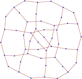
Figure 3: The MS graph $\Gamma^{a^{\prime}}_{34}(11)$

To identify/distinguish MS graphs:

A main method to identify graphs is the following.

Suppose that $\Gamma_{i}$ are the ($G_{i}$-invariant MS) graphs in $S^{3}$, and representations $\phi_{i}:\pi_{1}(\Gamma_{i}/G_{i})\cong G_{iA_{i}}\ast_{G_{ie_{i}}}G_{iB_{i}}\to G_{i}$ are induced by the orbifold embeddings, $i=1,2$.

If we have two isomorphisms $\eta$ and $\psi$ in the diagram above to make it commutative, where $\eta$ maps $G_{1A_{1}}$ to $G_{2A_{2}}$, $G_{1B_{1}}$ to $G_{2B_{2}}$, and $G_{1e_{1}}$ to $G_{2e_{2}}$, then clearly $\Gamma_{1}$ and $\Gamma_{2}$ are $G$-equivariant (abstract) graphs.

In practice, we will first give the presentations of the groups and then give the map between group generators and check if the map gives us a required group isomorphism.

We distinguish graphs by computing the graph invariants such as the number of vertices or edges, the degree of a vertex, the diameter of a graph and the girth (the length of a minimal loop) of a graph.

For complicated cases, we need computer programs to determine if maps are isomorphisms and to compute graph invariants.

Example 4.2.

The map $(\overline{u},\overline{u}_{l},\overline{u}_{r})\mapsto(\overline{v},\overline{v}_{l},\overline{v}_{r})$ in the proof of Theorem 4.4 is an isomorphism from $\pi_{1}(\mathcal{O}_{28})$ to $\pi_{1}(\mathcal{O}_{34})$.

⬇

f:=FreeGroup("x","y","z");

x:=f.1;

y:=f.2;

z:=f.3;

O28:=f/[x^5, y^2, z^2, (x*z)^3, (x*y)^2, (y*z^(-1))^2];

O34:=f/[x^2, y^3, z^2, (z*y)^2, (y*x*z)^2, (y*x*z*x)^3];

x:=O28.1; # x is an element in O28

y:=O28.2;

z:=O28.3;

r:=O34.1; # r is an element in O34

s:=O34.2;

t:=O34.3;

iso28:=IsomorphismPermGroup(O28); # pass to permutation group

iso34:=IsomorphismPermGroup(O34);

G28:=Image(iso28);

G34:=Image(iso34);

u:=Image(iso28,x*y*z^(-1)*x^(-1));

ul:=Image(iso28,x*z*x^(-1));

ur:=Image(iso28,x*z);

v:=Image(iso34,r^(-1));

vl:=Image(iso34,s^(-1)*t^(-1));

vr:=Image(iso34,t^(-1)r^(-1)s^(-1)r);

GroupHomomorphismByImages(G28,G34,[u,ul,ur],[v,vl,vr]);

Run the above codes in [GAP]. If it is an isomorphism, then [GAP] will give the correspondence between elements of the two groups. Otherwise the output will be “fail”. In this example the map is an isomorphism.

Example 4.3.

Compute the diameter and girth of $\Gamma^{a^{\prime}}_{34}(11)$.

⬇

Diameter[G34a’]

Girth[G34a’]

In Example 4.1, after input the list into [Mathematica], we just add the above two sentences. Then the computer will show that the diameter is $10$ and the girth is $12$.

4.2 Detailed classifications

Theorem 4.4.

(1) For each $g$, the MS graphs and their spatial graphs are:

• $g=11$. Four MS graphs, three with a unique spatial graph: $\Gamma_{28}^{a}({11})$, $\Gamma_{34}^{a}(11)$, $\Gamma_{34}^{a^{\prime}}(11)$; one with two spatial graphs $\Gamma_{28}^{a^{\prime}}(11)$ and $\Gamma_{34}^{b}(11,k)$;

• $g=241$. Four MS graphs, each with a unique spatial graph: $\Gamma_{38}^{a}(241)$, $\Gamma_{38}^{a^{\prime}}(241)$, $\Gamma_{38}^{b}(241,k)$, $\Gamma_{38}^{c}(241,k)$;

• $g=3,5,7,17,19,29,41,97,601,1681$. For each genus, two MS graphs, each with a unique (unknotted) spatial graph. The two graphs come from pairs of dual edges in the orbifolds listed in Theorem 3.3;

• $g=841$. Two MS graphs, each with a unique spatial graph: $\Gamma_{22D}^{a}(841)$, $\Gamma_{19}^{a}(841)$;

• $g=9,121,361$. For each genus, one MS graph, each with two spatial graphs: $\Gamma_{20C}^{a}(9)$ and $\Gamma_{20C}^{b}(9,k)$, $\Gamma_{22B}^{a}(121)$ and $\Gamma_{22B}^{b}(121,k)$, $\Gamma_{22C}^{a}(361)$ and $\Gamma_{22C}^{b}(361,k)$;

• $g=21,481$. For each genus, one MS graph, each with infinitely many different knotted spatial graphs: $\Gamma_{28}^{d}(21,k)\cong\Gamma_{34}^{c}(21,k)$, $\Gamma_{38}^{d}(481,k)$;

• For all other values of $g$, there is just one MS graph with a unique (unknotted) spatial graph.

(2) For each spatial MS graph $\Gamma$, there is a unique MS action. This is also true for each (abstract) MS graph $\Gamma$ except $\Gamma_{28}^{c}(29)\cong\Gamma_{15E}^{a}(29)$, where the actions correspond to $\Gamma_{28}^{c}(29)$ and $\Gamma_{15E}^{a}(29)$ are different.

Proof.

For each minimal graph $\Gamma$, denote the set of invariants by

$$\Lambda(\Gamma)=\{d_{k}(\Gamma),E(\Gamma),D(\Gamma),\mathcal{G}(\Gamma)\},$$

where $d_{k}$, $E$, $D$ and $\mathcal{G}$ denote the number of vertices of degree $k$ ($k=2,3,...$), the number of edges, the diameter, and the girth of $\Gamma$ respectively.

For a given $g$, $\gamma$ in $\mathcal{O}_{N}$ realizing $m_{g}$ are listed in Theorem 3.3, and $\Gamma_{N}^{\gamma}(g)$ are listed in Theorem 4.4. We will be able to picture all those graphs $\Gamma_{N}^{\gamma}(g)$ and to compute their invariants $\Lambda$ by the methods in last subsection, which are shown as in Appendix A (the pictures of $\Gamma$ with $E(\Gamma)>150$ are not given). As a result, graphs in the discussion with the same invariants $\Lambda$ are listed as below:

(i) $\Lambda(\Gamma_{28}^{c}(29))=\Lambda(\Gamma_{15E}^{a}(29))$,

(ii) $\Lambda(\Gamma_{28}^{a^{\prime}}(11))=\Lambda(\Gamma_{34}^{b}(11,k))$,

(iii) $\Lambda(\Gamma_{20C}^{a}(9))=\Lambda(\Gamma_{20C}^{b}(9,k))$,

(iv) $\Lambda(\Gamma_{22B}^{a}(121))=\Lambda(\Gamma_{22B}^{b}(121,k))$,

(v) $\Lambda(\Gamma_{22C}^{a}(361))=\Lambda(\Gamma_{22C}^{b}(361,k))$,

(vi) $\Lambda(\Gamma_{28}^{d}(21,k))=\Lambda(\Gamma_{34}^{c}(21,k))$ for any knotted dashed arcs $d$ and $c$,

(vii) $\Lambda(\Gamma_{38}^{d}(481,k))$ is constant for all knotted dashed arcs $d$.

Therefore for any genus which does not appear in the list (i)-(vii), Theorem 4.4 is proved, and for the remaining genera, we only need to consider the graphs listed in (i)-(vii).

At what follows, we use $\mathbb{Z}_{n}$ to denote the cyclic group with order $n$, use $D_{n}$ to denote the dihedral group with order $2n$, use $S_{n}$ to denote the permutation group with order $n!$, and use $A_{n}$ to denote the alternating group with order $n!/2$.

It is clear that $\Gamma_{28}^{c}(29)$ and $\Gamma_{15E}^{a}(29)$ are the same as abstract graphs (both are isomorphic to $K_{(2,30)}$, the complete bipartite graph with vertices partitioned into two subsets of cardinality 2 and 30), but their corresponding group actions are different: one group is isomorphic to $A_{5}\times\mathbb{Z}_{2}$ and the other is isomorphic to $D_{30}\times\mathbb{Z}_{2}$ . There is no diffeomorphism sending $(S^{3},\Gamma_{28}^{c}(29))$ to $(S^{3},\Gamma_{15E}^{a}(29))$ since at the vertex of degree 30 in $(S^{3},\Gamma_{15E}^{a}(29))$ all edges are tangent to some plane, and this is not the situation for $(S^{3},\Gamma_{28}^{c}(29))$. So $\Gamma_{28}^{c}(29)$ and $\Gamma_{15E}^{a}(29)$ are not the same spatial graph.

Two graphs in each pair of (ii), (iii), (iv), (v) are different spatial graphs, since one is knotted and the other is unknotted. We will prove that these two graphs are $G$-equivalent by the method discussed in last subsection, therefore finishing the proof of Theorem 4.4 for genus 11, 9, 121, and 361.

When $g=11$, we will prove that the representations induced by $a^{\prime}$ in $\mathcal{O}_{28}$ and $b$ in $\mathcal{O}_{34}$ are equivalent. Using the Wirtinger presentation, we have the following.

      

Figure 4: Presentations of $\pi_{1}(\mathcal{O}_{28})$ and $\pi_{1}(\mathcal{O}_{34})$

$\pi_{1}(\mathcal{O}_{28})$	$=$	$\langle x,y,z\mid x^{5},y^{2},z^{2},(xz)^{3},(xy)^{2},(yz^{-1})^{2}\rangle$,
$\pi_{1}(\mathcal{O}_{34})$	$=$	$\langle x,y,z\mid x^{2},y^{3},z^{2},(zy)^{2},(yxz)^{2},(yxzx)^{3}\rangle$.

$\pi_{1}(a^{\prime})\cong\pi_{1}(b)\cong D_{2}*_{\mathbb{Z}_{2}}D_{3}$. We choose three generators for $\pi_{1}(a^{\prime})$: $u$ is the generator of $D_{2}\cap D_{3}\cong{\mathbb{Z}}_{2}$, $u_{l}$ is an order $2$ element in $D_{2}$ different from $u$, $u_{r}$ is an order $3$ element in $D_{3}$. Similarly choose generators $v$, $v_{l}$, $v_{r}$ for $\pi_{1}(b)$. Then the equivalence is given by:

$\pi_{1}(a^{\prime})\rightarrow\pi_{1}(\mathcal{O}_{28})$	$:$	$(u,u_{l},u_{r})\mapsto(xyz^{-1}x^{-1},xzx^{-1},xz)$,
$\pi_{1}(b)\rightarrow\pi_{1}(\mathcal{O}_{34})$	$:$	$(v,v_{l},v_{r})\mapsto(x^{-1},y^{-1}z^{-1},z^{-1}x^{-1}y^{-1}x)$,
$\pi_{1}(a^{\prime})\rightarrow\pi_{1}(b)$	$:$	$(u,u_{l},u_{r})\mapsto(v,v_{l},v_{r})$,
$\pi_{1}(\mathcal{O}_{28})\rightarrow\pi_{1}(\mathcal{O}_{34})$	$:$	$(\overline{u},\overline{u}_{l},\overline{u}_{r})\mapsto(\overline{v},\overline{v}_{l},\overline{v}_{r})$.

Note that all the possible homomorphisms from a finitely presented group to a finite group are finitely many, and by using computer, for example [GAP], one can enumerate all such homomorphisms. Indeed we find the above homomorphisms by such a way.

When $g=9,121,361$, we need to prove that for $N=20C,22B,22C$ the representations induced by $a$ and $b$ are equivalent.

$N=20C$:

Figure 5: Presentation of $\pi_{1}(\mathcal{O}_{20C})$

$\pi_{1}(\mathcal{O}_{20C})=\langle x,y,z\mid x^{2},y^{3},z^{2},(y^{-1}x)^{2},(y^{-1}(xz)^{3}x)^{2},(y^{-1}xz^{-1})^{2}\rangle$.

$\pi_{1}(a)\cong\pi_{1}(b)\cong D_{2}*_{\mathbb{Z}_{2}}D_{3}$. We choose three generators for $\pi_{1}(a)$: $u$ is the generator of $D_{2}\cap D_{3}\cong\mathbb{Z}_{2}$, $u_{l}$ is an order $2$ element in $D_{2}$ different from $u$, $u_{r}$ is an order $3$ element in $D_{3}$. Similarly choose generators $v$, $v_{l}$, $v_{r}$ for $\pi_{1}(b)$. Then the equivalence is given by:

$\pi_{1}(a)\rightarrow\pi_{1}(\mathcal{O}_{20C})$	$:$	$(u,u_{l},u_{r})\mapsto(y^{-1}(xz)^{3}x,y^{-1}xz^{-1},y)$,
$\pi_{1}(b)\rightarrow\pi_{1}(\mathcal{O}_{20C})$	$:$	$(v,v_{l},v_{r})\mapsto((xz)^{2}x,y^{-1}(xz)^{3}x,xzxyxzx)$,
$\pi_{1}(a)\rightarrow\pi_{1}(b)$	$:$	$(u,u_{l},u_{r})\mapsto(v,v_{l},v_{r})$.

$N=22B$:

Figure 6: Presentation of $\pi_{1}(\mathcal{O}_{22B})$

$\pi_{1}(\mathcal{O}_{22B})=\langle x,y,z\mid x^{2},y^{3},z^{2},(y^{-1}x)^{2},(y^{-1}(xz)^{5}x)^{2},(y^{-1}xz^{-1})^{2}\rangle.$

$\pi_{1}(a)\cong\pi_{1}(b)\cong D_{2}*_{\mathbb{Z}_{2}}D_{3}$. We choose three generators for $\pi_{1}(a)$: $u$ is the generator of $D_{2}\cap D_{3}\cong\mathbb{Z}_{2}$, $u_{l}$ is an order $2$ element in $D_{2}$ different from $u$, $u_{r}$ is an order $3$ element in $D_{3}$. Similarly choose generators $v$, $v_{l}$, $v_{r}$ for $\pi_{1}(b)$. Then the equivalence is given by:

$\pi_{1}(a)\rightarrow\pi_{1}(\mathcal{O}_{22B})$	$:$	$(u,u_{l},u_{r})\mapsto(y^{-1}(xz)^{5}x,y^{-1}xz^{-1},y)$,
$\pi_{1}(b)\rightarrow\pi_{1}(\mathcal{O}_{22B})$	$:$	$(v,v_{l},v_{r})\mapsto((xz)^{4}x,y^{-1}xz^{-1},(xzxz)y(xzxz)^{-1})$,
$\pi_{1}(a)\rightarrow\pi_{1}(b)$	$:$	$(u,u_{l},u_{r})\mapsto(v,v_{l},v_{r})$.

$N=22C$:

Figure 7: Presentation of $\pi_{1}(\mathcal{O}_{22C})$

$\pi_{1}(\mathcal{O}_{22C})=\langle x,y,z\mid x^{2},y^{2},z^{2},(y^{-1}x)^{2},(y^{-1}(xz)^{3}x)^{2},(y^{-1}xz^{-1})^{5}\rangle.$

$\pi_{1}(a)\cong\pi_{1}(b)\cong D_{2}*_{\mathbb{Z}_{2}}D_{5}$. We choose three generators for $\pi_{1}(a)$: $u$ is the generator of $D_{2}\cap D_{5}\cong\mathbb{Z}_{2}$, $u_{l}$ is an order $2$ element in $D_{2}$ different from $u$, $u_{r}$ is an order $5$ element in $D_{5}$. Similarly choose generators $v$, $v_{l}$, $v_{r}$ for $\pi_{1}(b)$. Then the equivalence is given by:

$\pi_{1}(a)\rightarrow\pi_{1}(\mathcal{O}_{22C})$	$:$	$(u,u_{l},u_{r})\mapsto(x^{-1}y(zx)^{-3},x^{-1}yx,z^{-1}y^{-1}x)$,
$\pi_{1}(b)\rightarrow\pi_{1}(\mathcal{O}_{22C})$	$:$	$(v,v_{l},v_{r})\mapsto((xz)^{-2}z^{-1},x^{-1}y(zx)^{-3},zxy(xz)^{2})$,
$\pi_{1}(a)\rightarrow\pi_{1}(b)$	$:$	$(u,u_{l},u_{r})\mapsto(v,v_{l}*v,v_{r}^{2})$.

In the last two cases, (vi) and(vii), that is, $g=21$ and $481$, we need to prove that for $N=28,34$ and for $N=38$ all the representations induced by allowable dashed arcs are equivalent.

Notice that in these cases $\Gamma/G$ are all dashed arcs whose fundamental groups are isomorphic to ${\mathbb{Z}}_{2}\ast{\mathbb{Z}}_{3}$. By [Du2], the fundamental groups of orbifolds $\mathcal{O}_{28}$, $\mathcal{O}_{34}$ and $\mathcal{O}_{38}$ are isomorphic to $I\times\mathbb{Z}_{2}$, $A_{5}\times\mathbb{Z}_{2}$ and $\mathbf{I\times O}$ separately. The notations are explained as follows.

Let $O$ be the orientation-preserving isometry group of a regular octahedron (or a cube), and let $I$ be the orientation-preserving isometry group of a regular icosahedron (or a regular dodecahedron). Then clearly $O$ and $I$ belong to $SO(3)\subset SO(4)$. Hence they also act on $S^{3}$. $\mathbf{I\times O}$ is the two-sheeted covering of $I\times O$ under the two-to-one map $SO(4)\rightarrow SO(3)\times SO(3)$, and it acts on $S^{3}$. $A_{5}$ acts on a regular 4-simplex, which has 5 vertices, as the orientation-preserving isometry group. Hence it also acts on $S^{3}$. Finally the $\mathbb{Z}_{2}$ summand acts on $S^{3}$ as an antipodal map which commutes with the action given by $I$ or $A_{5}$. Note that as abstract groups $O\cong S_{4}$ and $I\cong A_{5}$. However, the actions given by $I$ and $A_{5}$ are different.

Then the results can be derived from Lemma 4.6 below. ∎

Remark 4.5.

In [Du2], $J$ is used to denote $I$ and notations $\mathbf{J\times_{J}J}$, $\mathbf{J\times^{*}_{J}J}$ and $\mathbf{J\times O}$ are used to denote the fundamental groups of $\mathcal{O}_{28}$, $\mathcal{O}_{34}$ and $\mathcal{O}_{38}$.

Lemma 4.6.

Suppose that $G$ is either $A_{5}\times\mathbb{Z}_{2}$ or $\mathbf{I\times O}$, and that $\{x,y\}$ and $\{z,w\}$ both generate $G$, where $x,z$ both have order $2$ and $y,w$ both have order $3$. Then the map $x\mapsto z,y\mapsto w$ gives an automorphism of $G$.

Proof.

Note that $I\cong A_{5}$ and $O\cong S_{4}$, hence $\mathbf{I\times O}$ is a two-sheeted covering of $A_{5}\times S_{4}$. Using the permutation representation, we may assume that $A_{5}$ acts on $\{1,2,3,4,5\}$, $\mathbb{Z}_{2}$ acts on $\{6,7\}$, and $S_{4}$ acts on $\{6,7,8,9\}$.

For $A_{5}\times{\mathbb{Z}}_{2}$, if an order $2$ element and an order $3$ element generate the group, then the two generators have forms like $(12)(34)(67)$ and $(135)$. It is not hard to see that the map between two such generating sets is an isomorphism.

For $A_{5}\times S_{4}$, if an order $2$ element and an order $3$ element generate the group, then the two generators have forms like $(12)(34)(69)$ and $(135)(678)$. Also the map between two such generating sets is an isomorphism, and $A_{5}\times S_{4}$ has the property stated in the lemma.

Now if an order $2$ element $x$ and an order $3$ element $y$ generate $\mathbf{I\times O}$, then the quotients $\overline{x}$ and $\overline{y}$ in $A_{5}\times S_{4}$ have the above forms. $\overline{y}$ has two preimages, one is $y$, the other has order $6$. Hence all such $y$’s are conjugate in $\mathbf{I\times O}$. Hence if $\{z,w\}$ satisfies the condition in the lemma, we can assume that $w=y$. Then considering the permutation representation and the two-to-one covering, the possible $z$ has $36$ choices.

Then using [GAP], one can confirm that all the $36$ choices give equivalent generator pairs. ∎

5 Maximum order of orientation-reversing case

Now we can consider maximum order problems for extendable actions on handlebodies and graphs for the general case, which allows group elements which reverse orientations.

Suppose $G$ acts on $(S^{3},U_{\epsilon}(\Gamma))$. Then for any $g\in G$, $g$ will preserve or reverse the orientations of $U_{\epsilon}(\Gamma)$ and $S^{3}$ simultaneously, therefore preserve or reverse the orientations of $\Sigma_{g}=\partial U_{\epsilon}(\Gamma)$ and $S^{3}$ simultaneously. That is to say, in graph and handlebody cases if there is an orientation-reversing element in $G$, $G$ must be of type $(-,-)$ on $(S^{3},\partial U_{\epsilon}(\Gamma))$ as defined in [WWZ]. Then the maximum order of extendable actions for orientation-reversing case will be $E_{g}(-,-)$, which is presented as Proposition 4.7 in [WWZ]. By definition, the action $G$ realizing $E_{g}(-,-)$ is faithful on $\partial U_{\epsilon}(\Gamma)$, therefore is faithful on the handlebody $U_{\epsilon}(\Gamma)$, but may not be faithful on the graph $\Gamma$.

Proposition 5.1.

(Proposition 4.7 of [WWZ] and its proof, also refer proof of Theorem 5.3 for the “Moreover” part) $E_{g}(-,-)$ are given as below:

$E_{g}(-,-)$	$g$
$24(g-1)$	$3,5,6,11,17,97,601$
$16(g-1)$	$7,73$
$40(g-1)/3$	$19$
$48(g-1)/5$	$41$
$60(g-1)/7$	$1681$
$8(\sqrt{g}+1)^{2}$	$k^{2}$, $k>1$
$8(g+1)$	the remaining numbers

Moreover for each $g$, $E_{g}(-,-)$ is realized (in the orbifold level) by a singular edge/dashed arc $\gamma$ of a 3-orbifold $\mathcal{O}_{N}$ shown as (a) or (b) in Figure 8, where a “reflection” of $\mathcal{O}_{N}$ fixes $\gamma$ (in (a), the fixed-point set of the reflection is the plane of the paper and in (b), the fixed-point set of the reflection is the indicated plane). We omit the labels here for convenience.

Figure 8: Orbifolds with reflections

Similar to Proposition 3.1, we have the following.

Proposition 5.2.

Suppose $G\subset O(4)$ acts on $(S^{3},\Gamma)$, $g\in G$ is not the identity of $G$ and its action on $\Gamma$ is the identity. Then $g$ must be a reflection about a geodesic 2-sphere $S^{2}$ in $S^{3}$, and $\Gamma\subset S^{2}$.

Proof.

By Proposition 3.1, we may assume that $g$ is orientation-reversing. By results in linear algebra, $\text{Fix}(g)$ is either a pair of points or a geodesic 2-sphere $S^{2}\subset S^{3}$. Since $\Gamma\subset\text{Fix}(g)$, $\text{Fix}(g)$ must be a geodesic $S^{2}(\supset\Gamma)$ and $g$ interchanges the two 3-balls separated by $S^{2}$. ∎

Suppose that the $G$-action on $\Gamma$ is not faithful. Then it is easy to see that if we $G$-equivariantly add some free edges to $\Gamma$ perpendicular to the geodesic $S^{2}$ containing $\Gamma$ to get $\Gamma^{*}$, then $G$ acts faithfully on $\Gamma^{*}$.

Now let $E(V_{g})$, $M^{*}_{g}$ and $M_{g}$ be the general maximum orders of extendable group actions on handlebodies, arbitrary graphs, and minimal graphs, of genus $g$ respectively. Then we have

Theorem 5.3.

(1) $m_{g}=OE_{g}\leq M_{g}\leq E(V_{g})=M^{*}_{g}.$

(2) $E(V_{g})=M^{*}_{g}$ are given in the following table.

$E(V_{g})=M^{*}_{g}$	$g$
$24(g-1)$	$2,3,4,5,6,11,17,97,601$
$16(g-1)$	$7,9,73$
$40(g-1)/3$	$16,19$
$12(g-1)$	$25,121,241$
$48(g-1)/5$	$41$
$60(g-1)/7$	$29,841,1681$
$8(\sqrt{g}+1)^{2}$	$k^{2}$, $k\neq 11$
$8(g+1)$	remaining numbers

(3) $M_{g}$ are given in the following table.

$M_{g}$	$g$
$24(g-1)$	$3,4,5,6,11,17,97,601$
$16(g-1)$	$7,9,73$
$40(g-1)/3$	$16,19$
$12(g-1)$	$2,25,121,241$
$48(g-1)/5$	$41$
$60(g-1)/7$	$29,841,1681$
$8(\sqrt{g}+1)^{2}$	$k^{2}$, $k\neq 11$
$8(g+1)>M_{g}\geq 4(g+1)$	remaining numbers

Proof.

(1) follows from the definitions, Theorem 1.1 and the paragraph after Proposition 5.2.

(2) Suppose that $G$ acts on $V_{g}$ realizing $E(V_{g})$. Then $G$ is either orientation-preserving or of the type $(-,-)$. To get the table in (2), we need only to compare tables in Theorem 1.1 (see also Remark 3.4) and in Proposition 5.1, where $E(V_{g})$ are chosen from the former for $g=25,121,241$, and from the later for the remaining $g$. Note that for table in (2) we can put 4, 9, 16, 25, 841 into the line of $k^{2}$, and 29 into the bottom line, then it has the form in the table of Proposition 5.1.

(3) By (2) and its proof, there is nothing to be further verified for $g=25,121,241$, and to prove (3), we need to verify the following

Claim for all remaining $g$, $M_{g}=E_{g}(-,-)$ if and only if $g$ is not in the bottom line and $g\neq 2$, and further more $M_{2}=12$.

(*) Note first that the “Moreover” part of Proposition 5.1 can be interpreted as that, for each $g$, $E_{g}(-,-)$ is realized by the orientation-preserving maximum symmetry of $\Gamma_{N}^{\gamma}(g)$ and reflections about geodesic 2-spheres which keep $\Gamma_{N}^{\gamma}(g)$ invariant. Therefore if $\Gamma_{N}^{\gamma}(g)$ does not stay in any geodesic 2-sphere, then the group action realizing $E_{g}(-,-)$ acts faithfully on $\Gamma_{N}^{\gamma}(g)$.

(**) Note then that $\Gamma_{N}^{\gamma}(g)\subset S^{3}$ does not stay in any geodesic 2-sphere in $S^{3}$ if a vertex $v$ of $\gamma$ in the singular set of $\mathcal{O}_{N}$ has three adjacent edges with index $(2,3,q)(q=3,4,5)$, since for any vertex $v^{\prime}$ of $\Gamma_{N}^{\gamma}(g)$ in $p^{-1}(v)$, where $p:S^{3}\to\mathcal{O}_{N}$ is the orbifold covering, the action of the stabilizer $St(v^{\prime})$ on a neighborhood of $v^{\prime}$ is the same as the isometry of some regular polyhedron, and adjacent edges of $v^{\prime}$ can not lie in any geodesic two sphere.

Now we are going to verify the “if” part of the claim by finding $\Gamma_{N}^{\gamma}(g)$ realizing $E_{g}(-,-)$ so that either $\gamma$ in $\mathcal{O}_{N}$ meets (**), or more directly $\Gamma_{N}^{\gamma}(g)$ is non-planar. These will be carried in (i) and (ii) below respectively. Therefore the group action $G$ realizing $E_{g}(-,-)$ acts faithfully on $\Gamma_{N}^{\gamma}(g)$.

(i) For $g=3,5,11,6,17,97,601,7,73,19,41,1681,29$, (we follow the order of their appearance in Theorem 3.3), we choose $\Gamma_{N}^{\gamma}(g)$ to be $\Gamma_{26}^{a}(3)$, $\Gamma_{27}^{a}(5)$, $\Gamma_{28}^{a}11)$, $\Gamma_{24}^{a}(6)$, $\Gamma_{29}^{a}(17)$, $\Gamma_{33}^{a^{\prime}}(97)$, $\Gamma_{30}^{a^{\prime}}(601)$, $\Gamma_{27}^{b}(7)$, $\Gamma_{25}^{a}(73)$, $\Gamma_{28}^{b}(19)$, $\Gamma_{29}^{b^{\prime}}(41)$, $\Gamma_{30}^{b^{\prime}}(1681)$, $\Gamma_{28}^{c^{\prime}}(29)$.

(ii) For all the squares $g=k^{2}$, we choose $\Gamma_{N}^{\gamma}(g)$ to be $\Gamma_{19}^{a}(k^{2})$, where the parameter $n$ in $\mathcal{O}_{19}$ is chosen to be $n=k+1$. As an abstract graph $\Gamma_{19}^{a}(k^{2})$ can be obtained from the complete bipartite graph $K_{(k+1,k+1)}$ by adding vertices. $K_{(k+1,k+1)}$ is a well-known non-planar graph, hence $\Gamma_{19}^{a}(k^{2})$ can not lie in a geodesic sphere.

For $g=2$ and the remaining cases, the graph realizing $E_{g}(-,-)$ is $\Gamma_{15E}^{a}(g)$, which is abstractly isomorphic to $K_{(2,g+1)}$, indeed lies in a geodesic 2-sphere, and the action on $\Gamma_{15E}^{a}(g)$ realizing $E_{g}(-,-)$ is not faithful (see also Appendix B).

By Theorem 2.1 and the proof of Theorem 1.1, the second biggest order of orientation-preserving extendable action on a genus 2 graph is $6$ (corresponds to ‘$a$’ in $\mathcal{O}_{01}$). Hence $M_{2}\leq 12$, and we have $M_{2}=12$. ∎

Example 5.4.

Suppose $g=pq$, $p$ is the smallest non trivial divisor of $g$. As the construction for $g=k^{2}$ for general case we can get a complete bipartite graph $K_{(p+1,q+1)}\subset S^{3}$ which has genus $g$ and on it there is an extendable group action with order $4(p+1)(q+1)$ which is bigger than $4(g+1)$ (see examples in [WWZZ1] and [WWZZ]). Clearly $K_{(p+1,q+1)}$ is non-planar.

Conjecture 5.5.

Suppose $g$ is neither a square number nor one of those finitely many $g$ listed in the table above. Then $M_{g}$ is $4(g+1)$ for prime $g$, and $4(p+1)(q+1)$ otherwise, where $pq=g$, $p$ is the smallest non trivial divisor of $g$.

Remark 5.6.

(1) The maximum order of finite group action on minimal graphs of genus $g$ is $2^{g}g!$ if $g>2$ and is 12 if $g=2$ [WZ].

(2) Any faithful action of finite group $G$ on a minimal graph $\Gamma$ of genus $g$ provides an embedding of $G$ into the out-automorphism group of the free group of rank $g$ for $g>1$.

Appendix A Table of MS graphs with invariants

This appendix contains some basic invariants of all the MS graphs.

In the following table, we denote by $d_{k}$ the number of vertices of degree $k$; $E$ the number of edges of a graph; $D$ the diameter of a graph; $\mathcal{G}$ the girth (or the length of a minimal loop) of a graph. Below we explain the last column which presents more standard names of those graphs if they have.

We use $K_{n}$ to denote the complete graph with $n$ vertices and $K_{m,n}$ to denote the complete bipartite graph with $m+n$ vertices. The generalized Petersen graph $G(n,k)$ is a graph with vertex set

$$\{u_{0},u_{1},\cdots,u_{n-1},v_{0},v_{1},\cdots,v_{n-1}\}$$

and edge set

$$\{u_{i}u_{i+1},u_{i}v_{i},v_{i}v_{i+k}\mid i=0,\cdots,n-1\}$$

where subscripts are to be read modulo $n$ and $k<n/2$.

In the following table, we use $\widetilde{K}_{n}$ (resp. $\widetilde{K}_{m,n}$, $\widetilde{G}(n,k)$) to denote the graph obtained by adding one degree $2$ vertex at the middle of each edge of $K_{n}$ (resp. $K_{m,n}$, $G(n,k)$). Moreover the precise meaning of “1-skeleton” in the last column also means a graph obtained by adding one degree $2$ vertex at the middle of each edge of that 1-skeleton.

name	number of vertices		E	D	$\mathcal{G}$	annotation
$|G|=12(g-1)$
$\Gamma_{15E}^{a}(2)$	$d_{2}=3$	$d_{3}=2$	6	2	4	$K_{2,3}$
$\Gamma_{26}^{a}(3)$	$d_{2}=4$	$d_{4}=2$	8	2	4	$K_{2,4}$
$\Gamma_{26}^{a^{\prime}}(3)$	$d_{2}=6$	$d_{3}=4$	12	4	6	$1$-skeleton of tetrahedron, $\widetilde{K}_{4}$
$\Gamma_{19}^{a}(4)$	$d_{2}=9$	$d_{3}=6$	18	4	8	$\widetilde{K}_{3,3}$
$\Gamma_{27}^{a}(5)$	$d_{2}=6$	$d_{6}=2$	12	2	4	$K_{2,6}$
$\Gamma_{27}^{a^{\prime}}(5)$	$d_{2}=12$	$d_{3}=8$	24	6	8	$1$-skeleton of cube, $\widetilde{G}(4,1)$
$\Gamma_{24}^{a}(6)$	$d_{2}=10$	$d_{4}=5$	20	4	6	$1$-skeleton of $4$-simplex, $\widetilde{K}_{5}$
$\Gamma_{20C}^{a}(9)$	$d_{2}=24$	$d_{3}=16$	48	8	12	Möbius-Kantor graph,
$\Gamma_{20C}^{b}(9,k)$						$\widetilde{G}(8,3)$
$\Gamma_{28}^{a}(11)$	$d_{2}=12$	$d_{12}=2$	24	2	4	$K_{2,12}$
$\Gamma_{28}^{a^{\prime}}(11)$	$d_{2}=30$	$d_{3}=20$	60	10	10	$1$-skeleton of dodecahedron,
$\Gamma_{34}^{b}(11,k)$						$\widetilde{G}(10,2)$
$\Gamma_{34}^{a}(11)$	$d_{2}=20$	$d_{4}=10$	40	6	8
$\Gamma_{34}^{a^{\prime}}(11)$	$d_{2}=30$	$d_{3}=20$	60	10	12	$\widetilde{G}(10,3)$, Desargues graph
$\Gamma_{29}^{a}(17)$	$d_{2}=24$	$d_{6}=8$	48	4	6	$1$-skeleton of $16$-cell
$\Gamma_{29}^{a^{\prime}}(17)$	$d_{2}=32$	$d_{4}=16$	64	8	8	$1$-skeleton of $4$-dim cube
$\Gamma_{21A}^{a}(25)$	$d_{2}=72$	$d_{3}=48$	144	12	16
$\Gamma_{33}^{a}(97)$	$d_{2}=288$	$d_{3}=192$	576	24	16
$\Gamma_{33}^{a^{\prime}}(97)$	$d_{2}=144$	$d_{6}=48$	288	8	8
$\Gamma_{22B}^{a}(121)$	$d_{2}=360$	$d_{3}=240$	720	22	20
$\Gamma_{22B}^{b}(121,k)$
$\Gamma_{38}^{a}(241)$	$d_{2}=480$	$d_{4}=240$	960	20	12
$\Gamma_{38}^{b}(241,k)$	$d_{2}=720$	$d_{3}=480$	1440	21	24
$\Gamma_{38}^{c}(241,k)$	$d_{2}=480$	$d_{4}=240$	960	14	16
$\Gamma_{38}^{a^{\prime}}(241)$	$d_{2}=720$	$d_{3}=480$	1440	30	18
$\Gamma_{30}^{a}(601)$	$d_{2}=720$	$d_{12}=120$	1440	10	6	$1$-skeleton of $600$-cell
$\Gamma_{30}^{a^{\prime}}(601)$	$d_{2}=1200$	$d_{4}=600$	2400	30	10	$1$-skeleton of $120$-cell
$|G|=8(g-1)$
$\Gamma_{27}^{b}(7)$	$d_{2}=8$	$d_{8}=2$	16	2	4	$K_{2,8}$
$\Gamma_{27}^{b^{\prime}}(7)$	$d_{2}=12$	$d_{4}=6$	24	4	6	$1$-skeleton of octahedron
$\Gamma_{21B}^{a}(49)$	$d_{2}=96$	$d_{4}=48$	192	10	12
$\Gamma_{25}^{a}(73)$	$d_{2}=96$	$d_{8}=24$	192	6	6	$1$-skeleton of $24$-cell
$|G|=20(g-1)/3$
$\Gamma_{19}^{a}(16)$	$d_{2}=25$	$d_{5}=10$	50	4	8	$\widetilde{K}_{5,5}$
$\Gamma_{28}^{b}(19)$	$d_{2}=20$	$d_{20}=2$	40	2	4	$K_{2,20}$
$\Gamma_{28}^{b^{\prime}}(19)$	$d_{2}=30$	$d_{5}=12$	60	6	6	$1$-skeleton of icosahedron
$\Gamma_{22C}^{a}(361)$	$d_{2}=600$	$d_{5}=240$	1200	14	12
$\Gamma_{22C}^{b}(361,k)$
$|G|=6(g-1)$
$\Gamma_{28}^{d}(21,k)$	$d_{2}=960$	$d_{3}=40$	120	12	16
$\Gamma_{34}^{c}(21,k)$
$\Gamma_{38}^{d}(481,k)$	$d_{2}=1440$	$d_{3}=960$	2880	36	24
$|G|=24(g-1)/5$
$\Gamma_{29}^{b}(41)$	$d_{3}=32$	$d_{4}=24$	96	6	6
$\Gamma_{29}^{b^{\prime}}(41)$	$d_{4}=16$	$d_{8}=8$	64	4	4
$|G|=30(g-1)/7$
$\Gamma_{30}^{b}(1681)$	$d_{3}=1200$	$d_{5}=720$	3600	20	6
$\Gamma_{30}^{b^{\prime}}(1681)$	$d_{4}=600$	$d_{20}=120$	2400	10	4

name	number of vertices		E	D	$\mathcal{G}$	annotation
$|G|=4(\sqrt{g}+1)^{2}$ for $g=k^{2},k\neq 3,5,7,11,19,41$
$\Gamma_{22D}^{a}(841)$	$d_{3}=600$	$d_{5}=360$	1800	12	8
$\Gamma_{19}^{a}(841)$	$d_{2}=900$	$d_{30}=60$	1800	4	8	$\widetilde{K}_{30,30}$
$\Gamma_{19}^{a}(k^{2})$	$d_{2}=(k+1)^{2}$	$d_{k+1}=2(k+1)$	$2(k+1)^{2}$	4	8	$\widetilde{K}_{k+1,k+1}$
$|G|=4(g+1)$ for remaining $g$
$\Gamma_{28}^{c}(29)$	$d_{2}=30$	$d_{30}=2$	60	2	4	$K_{2,30}$
$\Gamma_{15E}^{a}(29)$
$\Gamma_{28}^{c^{\prime}}(29)$	$d_{3}=20$	$d_{5}=12$	60	6	4
$\Gamma_{15E}^{a}(g)$	$d_{2}=g+1$	$d_{g+1}=2$	$2g+2$	2	4	$K_{2,g+1}$

Even if our computer program can produce any MS graph above, it is hard to understand the picture when the number of its edges is very large. Following are the pictures of abstract MS graphs with less than $150$ edges and not of type $K_{2,n}$ (there are many figures of this type which are very easy to understand).

$\Gamma_{26}^{a^{\prime}}(3)$

$\Gamma_{19}^{a}(4)$

$\Gamma_{27}^{a^{\prime}}(5)$

$\Gamma_{24}^{a}(6)$

$\Gamma_{20C}^{a}(9)\cong\Gamma_{20C}^{b}(9,k)$

$\Gamma_{28}^{a^{\prime}}(11)\cong\Gamma_{34}^{b}(11,k)$

$\Gamma_{34}^{a}(11)$

$\Gamma_{34}^{a^{\prime}}(11)$

$\Gamma_{29}^{a}(17)$

$\Gamma_{29}^{a^{\prime}}(17)$

$\Gamma_{21A}^{a}(25)$

$\Gamma_{27}^{b^{\prime}}(7)$

$\Gamma_{19}^{a}(16)$

$\Gamma_{28}^{b^{\prime}}(19)$

$\Gamma_{28}^{d}(21,k)$

$\Gamma_{29}^{b}(41)$

$\Gamma_{29}^{b^{\prime}}(41)$

$\Gamma_{28}^{c^{\prime}}(29)$

Appendix B Description of spatial MS graphs

With one point removed, the unit sphere $S^{3}\subset E^{4}$ will be mapped to $\mathbb{R}^{3}$ by a stereographic projection. Each MS spacial graph in $S^{3}$ consists of geodesic segments as edges, which are mapped to circles in $\mathbb{R}^{3}$.

This appendix contains the pictures in $\mathbb{R}^{3}$ which are stereographic projections of some spatial MS graphs in $S^{3}$. Those pictures present the geometrical shapes of those spatial MS graphs, and possibly also some beauty and complexity provided by geometry and computer programs.

For intuitive descriptions of the corresponding symmetries for many cases, please see also the last sections of [WWZZ1] and [WWZZ].

Below we present the shape of those graphs: Two infinite series, some spacial graphs related to 3- and 4-dimensional regular polyhedra (2- and 3-dimensional spherical tessellation), finally one example for the knotted case.

In many cases, when we delete the vertices of degree $2$, the graph will become a classical graph such as complete graph, complete bipartite graph, 1-skeletons of regular polyhedra and so on. The word “essentially” will mean that the vertices of degree $2$ are deleted.

The first two figures give the general case, the two infinite series.

$\Gamma_{15E}^{a}(g)$ is the complete bipartite graph $K_{(2,g+1)}$. $\Gamma_{19}^{a}(k^{2})$ is essentially the complete bipartite graph $K_{(k+1,k+1)}$. The following figures are for $g=8$ and $k=4$.

Next we present figures related to regular 3-dimensional polyhedra.

$\Gamma_{26}^{a^{\prime}}(3)$, $\Gamma_{27}^{a^{\prime}}(5)$, $\Gamma_{28}^{a^{\prime}}(11)$, $\Gamma_{27}^{b^{\prime}}(7)$ and $\Gamma_{28}^{b^{\prime}}(19)$ are essentially the 1-skeletons of the regular tetrahedron, the regular cube, the regular dodecahedron, the regular octahedron and the regular icosahedron respectively. If we connect the vertices and the face centers of the regular dodecahedron (or the regular icosahedron) by geodesic segments in the faces, then we will get the graph $\Gamma_{28}^{c^{\prime}}(29)$. Note that the dual graphs of the above six graphs are all dipole graphs with vertices at the center of the polyhedra and the infinity. The following figures are for $\Gamma_{26}^{a^{\prime}}(3)$, $\Gamma_{27}^{a^{\prime}}(5)$ and $\Gamma_{28}^{a^{\prime}}(11)$ respectively.

Consider the Hopf fibration $S^{3}\rightarrow S^{2}$. Fixed a point in $S^{3}$, the above six graphs in $S^{2}$ can be lifted piecewise, and we can get six graphs in $S^{3}$, which are essentially $\Gamma_{20C}^{a}(9)$, $\Gamma_{21A}^{a}(25)$, $\Gamma_{22B}^{a}(121)$, $\Gamma_{21B}^{a}(49)$, $\Gamma_{22C}^{a}(361)$ and $\Gamma_{22D}^{a}(841)$, corresponding to $\Gamma_{26}^{a^{\prime}}(3)$, $\Gamma_{27}^{a^{\prime}}(5)$, $\Gamma_{28}^{a^{\prime}}(11)$, $\Gamma_{27}^{b^{\prime}}(7)$, $\Gamma_{28}^{b^{\prime}}(19)$ and $\Gamma_{28}^{c^{\prime}}(29)$. The following figures are for $\Gamma_{20C}^{a}(9)$ and $\Gamma_{21A}^{a}(25)$ respectively.

The following graphs are related to 4-dimensional regular polyhedra.

$\Gamma_{24}^{a}(6)$ is essentially the 1-skeleton of a regular 4-simplex (or a regular 5-cell). If we connect the vertices and the 3-dimensional face centers of the 4-simplex by line segments in the faces, then we will get $\Gamma_{34}^{a}(11)$. The dual graph $\Gamma_{34}^{a^{\prime}}(11)$ can be obtained by connecting the 1-dimensional face centers and the 2-dimensional face centers of the 4-simplex. The following figures are for $\Gamma_{24}^{a}(6)$, $\Gamma_{34}^{a}(11)$ and $\Gamma_{34}^{a^{\prime}}(11)$ respectively.

$\Gamma_{29}^{a^{\prime}}(17)$ is essentially the 1-skeleton of a regular 4-cube (or a regular 8-cell). Its dual graph $\Gamma_{29}^{a}(17)$ is essentially the 1-skeleton of a regular 16-cell which is the dual polyhedron of the 4-cube. The following figures are for $\Gamma_{29}^{a^{\prime}}(17)$ and $\Gamma_{29}^{a}(17)$ respectively.

For other regular polyhedra, there are similar constructions. $\Gamma_{30}^{a^{\prime}}(601)$ is essentially the 1-skeleton of a regular 120-cell. Its dual graph $\Gamma_{30}^{a}(601)$ is essentially the 1-skeleton of a regular 600-cell which is the dual polyhedron of the 120-cell. $\Gamma_{25}^{a}(73)$ is essentially the 1-skeleton of a regular 24-cell, which is a self-dual polyhedron. If we connect the vertices and the 3-dimensional face centers of the 4-cube (resp. 120-cell), then we will get the graph $\Gamma_{29}^{b^{\prime}}(41)$ (resp. $\Gamma_{30}^{b^{\prime}}(1681)$). If we connect the 1-dimensional face centers and the 2-dimensional face centers of the 4-cube (resp. 120-cell), then we will get the graph $\Gamma_{29}^{b}(41)$ (resp. $\Gamma_{30}^{b}(1681)$).

The remaining spatial MS graph of genus $11$ is $\Gamma_{34}^{b}(11,k)$. It comes from a certain edge in the fundamental domain of the corresponding group action, see Example 7.4 of [WWZZ]. The following figure is for $\Gamma_{34}^{b}(11,k)$.

Remark B.1.

Contrary to the case of abstract MS graph, there is no uniform way to picture all the spatial MS graphs. In each case, one has to analyse the isometries of the groups so geometry is involved. To get a picture, we usually first picture a part of the graph, then apply the group action to it to get the whole graph. The quaternion representation of the group is the key for many cases. For more details about finite subgroups of $SO(4)$ one can see [CS], [Du1] and [Du2]. The code for [Mathematica] of the graphs can be found in Appendix C of [Wa, pages 112-138]. Even as a Ph.D thesis in Peking University, [Wa] is written in Chinese, but the code part could still be understood.

Chao Wang, School of Mathematical Sciences, University of Science and Technology of China, Hefei, 230026 CHINA
E-mail address: chao_wang_1987@126.com

Shicheng Wang, School of Mathematical Sciences, Beijing 100871 CHINA
E-mail address: wangsc@math.pku.edu.cn

Yimu Zhang, Mathematics School, Jilin University, Changchun, 130012 CHINA
E-mail address: zym534685421@126.com

Bruno Zimmermann, Universita degli Studi di Trieste, Trieste, 34100 Trieste ITALY
E-mail address: zimmer@units.it

References

- [BMP] M. Boileau, S. Maillot, J. Porti, Three-dimensional orbifolds and their geometric structures, Panoramas et Synthèses 15. Société Mathématique de France, Paris 2003.
- [CS] J. H. Conway, D. A. Smith. On quaternions and octonions: their geometry, arithmetic, and symmetry. A K Peters, Ltd., Natick, MA, 2003.
- [Du1] W.D. Dunbar, Geometric orbifolds, Rev. Mat. Univ. Complut. Madrid 1 (1988), 67-99.
- [Du2] W.D. Dunbar, Nonfibering spherical 3-orbifolds, Trans. Amer. Math. Soc. 341 (1994), 121-142.
- [MMZ] D. McCullough, A. Miller, B. Zimmermann, Group actions on handlebodies, Proc. London Math. Soc. (3) 59 (1989), 373-416.
- [Pe] G. Perelman. The entropy formula for the Ricci flow and its geometric applications (eprints arXiv: math/0211159); Ricci flow with surgery on three-manifolds (eprints arXiv: math/0303109); Finite extinction time for the solutions to the Ricci flow on certain three-manifolds (eprints arXiv: math/0307245)
- [Se] J. P. Serre. Trees, Translated from the French by John Stillwell. Springer-Verlag, Berlin-New York, 1980.
- [Th] W. P. Thurston, The geometry and topology of three-manifolds, Lecture Notes, Princeton University 1978. (http://library.msri.org/books/gt3m/)
- [Wa] C. Wang, Ph.D Thesis, Peking University, 2014.
- [WWZZ1] C. Wang, S. C. Wang, Y. M. Zhang, B. Zimmermann, Extending finite group actions on surfaces over , Topol. Appl. 160 (16) (2013) 2088-2103.
- [WWZZ] C. Wang, S. C. Wang, Y. M. Zhang, B. Zimmermann, Embedding surfaces into with maximum symmetry, Groups Geom. Dyn. 9 (2015), no. 4, 1001–1045.
- [WWZ] C. Wang, S. C. Wang, Y. M. Zhang, Maximum orders of extendable actions on surfaces, Acta Math. Sin. (Engl. Ser.) 32 (2016), no. 1, 54 C68.
- [WZ] S. C. Wang, B. Zimmermann, The maximum order of finite groups of outer automorphisms of free groups. Math. Z. 216 (1994), no. 1, 83–87.
- [GAP] The GAP Group, GAP — Groups, Algorithms, and Programming, Version 4.4.12; 2008 (http://www.gap-system.org).
- [Mathematica] Wolfram Research, Inc., Mathematica, Version 6.0, Champaign, IL (2007).