Systematic investigations of deep sub-barrier fusion reactions using an adiabatic approach

Abstract

Background

At extremely low incident energies, unexpected decreases in fusion cross sections, compared to the standard coupled-channels (CC) calculations, have been observed in a wide range of fusion reactions. These significant reductions of the fusion cross sections are often referred to as the fusion hindrance. However, the physical origin of the fusion hindrance is still unclear.

Purpose

To describe the fusion hindrance based on an adiabatic approach, I propose a novel extension of the standard CC model by introducing a damping factor that describes a smooth transition from sudden to adiabatic processes. I demonstrate the performance of this model by systematically investigating various deep sub-barrier fusion reactions.

Method

I extend the standard CC model by introducing a damping factor into the coupling matrix elements in the standard CC model. This avoids double counting of the CC effects, when two colliding nuclei overlap one another. I adopt the Yukawa-plus-exponential (YPE) model as a basic heavy ion-ion potential, which is advantageous for a unified description of the one- and two-body potentials. For the purpose of these systematic investigations, I approximate the one-body potential with a third-order polynomial function based on the YPE model.

Results

Calculated fusion cross sections for the medium-heavy mass systems of ⁶⁴Ni + ⁶⁴Ni, ⁵⁸Ni + ⁵⁸Ni, and ⁵⁸Ni + ⁵⁴Fe, the medium-light mass systems of ⁴⁰Ca + ⁴⁰Ca, ⁴⁸Ca + ⁴⁸Ca, and ²⁴Mg + ³⁰Si, and the mass-asymmetric systems of ⁴⁸Ca + ⁹⁶Zr and ¹⁶O + ²⁰⁸Pb are consistent with the experimental data. The astrophysical S factor and logarithmic derivative representations of these are also in good agreement with the experimental data. The values obtained for the individual radius and diffuseness parameters in the damping factor, which reproduce the fusion cross sections well, are nearly equal to the average value for all the systems.

Conclusions

Since the results calculated with the damping factor are in excellent agreement with the experimental data in all systems, I conclude that the smooth transition from the sudden to adiabatic processes occurs and that a coordinate-dependent coupling strength is responsible for the fusion hindrance. In all systems, the potential energies at the touching point $V_{\rm Touch}$ strongly correlate with the incident threshold energies for which the fusion hindrance starts to emerge, except for the medium-light mass systems.

I Introduction

Heavy-ion fusion reactions are an important probe to investigate the fundamental features of the macroscopic tunneling for many-body quantum systems. The Coulomb barrier is formed when a projectile approaches a target, because of the strong cancellation between the Coulomb repulsion and nuclear attractive forces. Fusion occurs when the projectile penetrates through this Coulomb barrier. The fusion reaction at incident energies around the Coulomb barrier is called the sub-barrier fusion reaction. An important observation of the sub-barrier fusion reactions is that the measured fusion cross sections exhibit strong enhancements compared to estimations using a simple one-dimensional model DHRS98 . These enhancements have been accounted for in terms of strong couplings between the relative motion of colliding nuclei and the intrinsic degrees of freedom, such as the collective vibrations of the target and/or projectile. In this context, the coupled-channels (CC) model based on this picture has been successful in describing these enhancements Bal98 ; Hagino12 .

Because of recent progress in experimental techniques, it is possible to precisely measure the fusion cross sections down to extremely low incident energies, the so-called “deep sub-barrier energies”. The experimental data revealed that significant decreases in the fusion cross sections at deep sub-barrier energies, compared to the standard CC calculations, emerge in a wide range of reaction systems Jiang02 ; Jiang04 ; Jiang06 (see Ref. Back14 for details). These significant decreases in the fusion cross section are often referred to as fusion hindrance. Below, the incident energy for which the fusion hindrance starts to emerge is referred to as “the incident threshold energy for fusion hindrance”.

A key quantity for understanding the fusion hindrance is the potential energy at the touching point $V_{\rm Touch}$, which strongly correlates with the incident threshold energy for fusion hindrance ich07-2 . When the incident energy is lower than $V_{\rm Touch}$, the inner turning point of the potential energy becomes inside the touching point (see Fig. 1). Namely, the projectile is still in a classically forbidden region when the two colliding nuclei touch with each other. As a result, the colliding nuclei must penetrate through a residual barrier with an overlapping configuration before fusion occurs. Thus, the fusion hindrance would be associated with the dynamics in the overlapping region of the two colliding nuclei.

To describe the fusion hindrance associated with the dynamics in the overlapping region, two approaches with different assumptions that contradict one another have been proposed Back14 . One is the sudden approach proposed by Mişicu and Esbensen mis06 , which assumes that fusion occurs rapidly. They considered the Pauli principle effect that acts when two colliding nuclei overlap one another. Thus, they constructed a heavy ion-ion potential with a shallow potential pocket based on the frozen-density approximation. They systematically investigated various reaction systems to test the performance of the sudden model Esb07 ; Esb10 ; mis11 ; Monta12 ; Jiang14 .

The other is the adiabatic approach proposed by Ichikawa et al. ich07-1 ; ich09 , which assumes that fusion slowly occurs and that neck formation between two colliding nuclei occurs in the overlapping region. In these considerations, the sudden and adiabatic processes are smoothly jointed by phenomenologically introducing a damping factor in the coupling form factor to avoid double counting of the CC effects. Later, it was shown that the physical origin of this damping factor is the damping of quantum vibrations near the touching point of two colliding nuclei using the random-phase approximation (RPA) method for the ¹⁶O + ¹⁶O, ⁴⁰Ca + ⁴⁰Ca, and ¹⁶O +²⁰⁸Pb systems ich13 ; ich15 .

Another approach, different from the CC model, has recently been developed to describe heavy-ion fusion reactions based on self-consistent mean-field theory Back14 . In this approach, the time-dependent Hatree-Fock (TDHF) method is often used to extract an adiabatic heavy ion-ion potential. Umar and Oberacker proposed the density-constrained TDHF method and demonstrated the energy-dependent heavy ion-ion potential with inertia mass relative to the center-of-mass distance between two colliding nuclei Umar06 ; Umar09 ; Umar14 ; Keser12 . Although in this approach, any input parameters are not required to calculate fusion cross sections once one determines an energy-density functional, its mechanism for the fusion hindrance is still unclear.

In this paper, I systematically investigate the fusion hindrance using the adiabatic approach to test the model’s performance in various reaction systems. Later, I show that the adiabatic approach works very well in many systems, strongly indicating that indeed the smooth transition from sudden to adiabatic processes occurs in deep sub-barrier fusion reactions, i.e. this coordinate-dependent coupling strength is responsible for the fusion hindrance. I also show that a difference between the adiabatic and sudden models appears in the average angular momentum of compound nuclei. I also discuss the strong correlation between $V_{\rm Touch}$ and the incident threshold energy for fusion hindrance.

The rest of the paper is organized as follows. In Section II, I describe the theoretical framework and how to construct a heavy ion-ion potential. In Section III, I present the results of the systematic calculations by applying the adiabatic approach for the medium-heavy, medium-light, and mass-asymmetric systems. In Section IV, I discuss the average angular momentum of compound nuclei calculated with the adiabatic and sudden models, and the correlation between $V_{\rm Touch}$ and the threshold incident energy for activating the fusion hindrance. I summarize my studies in Section V.

II THEORETICAL FRAMEWORK

II.1 Concept of a smooth transition from sudden to adiabatic processes

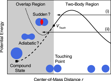
Figure 1: (Color online) Schematic picture of a heavy ion-ion potential versus the center-of-mass distance $r$ between colliding nuclei. The solid circle and square indicate the touching point of the colliding nuclei and its compound state, respectively. The gray area represents the overlapping region of the colliding nuclei. The dashed and dotted lines indicate the potential energy curves for the adiabatic and sudden processes, respectively.

Here, I discuss how to describe the fusion hindrance based on the adiabatic approach and show a concept of smooth transition from sudden to adiabatic processes.

An important aspect of fusion reactions at deep sub-barrier incident energies is that the inner turning point of a heavy ion-ion potential would be located deep within the touching point of the colliding nuclei. Figure 1 shows a schematic picture of a heavy ion-ion potential versus incident energies in a fusion reaction. The solid line indicates a potential energy curve in the two-body region. The solid circle indicates the potential energy at the touching point $V_{\rm Touch}$ of the colliding nuclei. The gray area represents the overlapping region of the colliding nuclei. At incident energies around the Coulomb barrier, the inner turning point is still far outside of the touching point [line (i) in Fig. 1]. At these energies, one usually assumes that a compound nucleus is automatically formed once the projectile penetrates the Coulomb barrier because of strong nuclear attractive forces in the classically allowed region. On the other hand, at incident energies below $V_{\rm Touch}$, the inner turning point appears more deeply within the touching point [line (ii) in Fig. 1]. Namely, the projectile is still in the classically forbidden region when the colliding nuclei touch one another.

After touching, a composite system is formed, which evolves in the classically forbidden region toward its compound state by overlapping between projectile- and target-like nuclei. Since this involves the penetration of a residual Coulomb barrier, fusion cross sections are naturally hindered by the tunneling factor. In Ref. ich07-2 , a strong correlation between $V_{\rm Touch}$ and the incident threshold energy for fusion hindrance is found by systematically investigating various experimental data. Thus, the dynamics after the nuclei collide plays an essential role in significantly decreasing the fusion cross section at deep sub-barrier incident energies.

A description for the evolution toward the compound state strongly depends on which model is employed in the overlapping region. There are mainly two assumptions that contradict one another. One is the sudden approach, where fusion rapidly occurs. Here, the potential energy curve would have a shallow potential pocket due to the strong overlapping of the two colliding nuclei [dotted line in Fig. 1]. The other is the adiabatic approach, where the density distribution of the composite system evolves with the lowest energy configuration [dashed line in Fig. 1]. In this paper, I focus on applying the adiabatic process to the standard CC model framework.

However, one cannot directly apply the adiabatic potential calculated with the lowest energy configuration to the standard CC model, because its direct application leads to double counting of the CC effects. Channel coupling already includes many effects of the adiabatic process, including neck formation between the colliding nuclei. To avoid such double counting, I developed a full quantum mechanical model, whereby the CC effect in the two-body system is smoothly jointed to the adiabatic potential tunneling for the one-body system.

In the CC calculations, one often employs the incoming wave boundary condition in order to simulate a compound nucleus formation. To construct an adiabatic potential model with it, I assume the following conditions: (1) before the target and projectile touch one another, the standard CC model in the two-body system works well; (2) after the target and projectile appreciably overlap one another, the fusion process is governed by a single adiabatic one-body potential, whereby the excitation on the adiabatic base is neglected; and (3) the transition from the two- to one-body treatments occurs near the touching point, where all physical quantities are smoothly joined. These are the important conditions, which should be taken into account in the adiabatic approach under the framework of the CC model.

II.2 An extension of the standard coupled-channel model

Before describing an extension of the standard CC model, taking into account the adiabatic process, I first briefly describe the standard CC model (for details see Refs. Esb87 ; ccfull ; Hagino12 ).

For heavy-ion fusion reactions, the no-Coriolis approximation is often used ccfull ; Hagino12 . Here, one can replace the angular momentum of the relative motion of colliding nuclei in each channel by the total angular momentum, $J$. For simplicity, the index $J$ is suppressed and a simplified notation $n=\{\alpha,\ell,I\}$ is used in the following, where $\alpha$ denotes any quantum numbers separate from the angular momenta, and $\ell$ and $I$ denote the orbital and intrinsic angular momenta, respectively. The CC equations ccfull ; Hagino12 are then given by

$$\Biggl{[}-\frac{\hbar^{2}}{2\mu}\frac{d^{2}}{dr^{2}}+\frac{J(J+1)\hbar^{2}}{2\mu r^{2}}+V^{(0)}(r)+\epsilon_{n}-E\Biggr{]}u_{n}(r)\\ +\sum_{m}V_{nm}(r)u_{m}(r)=0,$$ (1)

where $r$ is the radial component of the relative motion coordinate, $\mu$ is the reduced mass, $E$ is the incident energy in the center-of-mass frame, and $\epsilon_{n}$ is the excitation energy of the $n$-th channel. A bare nuclear potential $V^{(0)}$ consisting of the Coulomb and nuclear interactions is given by $V^{(0)}(r)=Z_{T}Z_{P}e^{2}/r+V_{N}^{(0)}(r)$. The matrix elements of the coupling Hamiltonian $V_{nm}$ are calculated with the collective model including the Coulomb and nuclear components.

The CC equations are solved by imposing the incoming wave boundary condition ccfull ; Hagino12 at the minimum of the potential pocket $r_{\rm min}$ inside the Coulomb barrier. This condition is expressed as

$$u_{n}(r) \sim T_{n}\exp\left(-i\int_{r_{\rm min}}^{r}k_{n}(r^{\prime})dr^{\prime}\right) (r\leq r_{\rm min})$$ (2)

$$=H_{J}^{(-)}(k_{n}r)\delta_{n,0}+S_{n}H_{J}^{(+)}(k_{n}r) (r\rightarrow\infty),$$ (3)

where $S_{n}$ are the $S$ matrix, $T_{n}$ are the transmission coefficients, and $H^{(+)}$ and $H^{(-)}$ are the outgoing and incoming Coulomb wave functions, respectively. The local wave number for the $n$-th channel $k_{n}$(r) is given by

$$k_{n}(r)=\sqrt{\frac{2\mu}{\hbar^{2}}\left(E-\epsilon_{n}-\frac{J(J+1)\hbar^{2}}{2\mu r^{2}}-V^{(0)}(r)-V_{nm}(r)\right)}.$$ (4)

By taking a summation over all possible intrinsic states, the inclusive penetrability is given by

$$P_{J}(E)=\sum_{n}\frac{k_{n}(r_{\rm min})}{k_{0}}|T_{n}|^{2},$$ (5)

where $k_{n}=k_{n}(r=\infty)$ and the ground state of the target nucleus is denoted by $n=0$. The fusion cross section $\sigma_{\rm fus}$ is thus obtained as

$$\sigma_{\rm fus}(E)=\frac{\pi}{k^{2}}\sum_{J}(2J+1)P_{J}(E).$$ (6)

In coupling matrix elements, I consider only vibrational couplings in this paper. The nuclear coupling Hamiltonian can be generated by changing the target radius in the nuclear potential of $V_{N}^{(0)}$ to a dynamical operator $R_{0}\rightarrow R_{0}+\hat{O}_{\lambda}$. Therefore, the nuclear coupling Hamiltonian is given by $V_{N}(r,\hat{O}_{\lambda})=V_{N}^{(0)}(r-\hat{O}_{\lambda})$ ccfull ; Hagino12 . For the vibrational coupling, the operator $\hat{O}_{\lambda}$ is given by $\hat{O}_{\lambda}=\beta_{\lambda}/\sqrt{4\pi}\cdot R_{T}(\alpha_{\lambda 0}^{\dagger}+\alpha_{\lambda 0})$, where $\alpha_{\lambda 0}^{\dagger}$ and $\alpha_{\lambda 0}$ are the creation and annihilation operators of the phonons, respectively, and $R_{T}$ is the radius of the target nucleus. Here, the eigenvalues $\lambda_{\alpha}$ and the eigenvectors $|\alpha\rangle$ of $\hat{O}_{\lambda}$ are given by $\hat{O_{\lambda}}|\alpha\rangle=\lambda_{\alpha}|\alpha\rangle$. The deformation parameter $\beta_{\lambda}$ is an input parameter and can be estimated from an experimental transition probability $B(E\lambda)$ which is given by

$$\beta_{\lambda}=\frac{4\pi}{3Z_{T}R_{T}^{\lambda}}\sqrt{\frac{B(E\lambda)\uparrow}{e^{2}}},$$ (7)

where $Z_{T}$ is the proton number and $e$ is the elementary charge.

The matrix elements of the nuclear coupling Hamiltonian are expanded by the eigenvalues and eigenvectors ccfull ; Hagino12 ; Esb87 , and thus are defined as

$$V^{(N)}_{nm} =\langle n|V_{N}(r,\hat{O}_{\lambda})|m\rangle-C_{0}(r)$$

$$=\sum_{\alpha}\langle n|\alpha\rangle\langle\alpha|m\rangle V_{N}(r,\lambda_{\alpha})-C_{0}(r),$$ (8)

where $C_{0}$ is the coupling constant given by $C_{0}(r)=\langle 0|V_{N}(r,\hat{O}_{\lambda})|0\rangle$. In Ref. Esb87 , the nuclear coupling potential $V_{N}(r,\lambda_{\alpha})=V_{N}^{(0)}(r-\lambda_{\alpha})$ is expanded by $\lambda_{\alpha}$ and is taken up to the second order of $\lambda_{\alpha}$, which is given by

$$V_{N}(r,\lambda_{\alpha})=V_{N}^{\rm(0)}(r)-\frac{dV_{N}^{\rm(0)}}{dr}\lambda_{\alpha}+\frac{1}{2}\frac{d^{2}V_{N}^{\rm(0)}}{dr^{2}}\lambda_{\alpha}^{2}.$$ (9)

Thus, one can calculate $V_{nm}^{(N)}$ with Eqs. (8) and (9). The Coulomb coupling matrix elements $V^{(C)}_{nm}$ are similarly calculated using the linear coupling approximation ccfull ; Hagino12 . The total coupling matrix elements are given by the sum of $V_{nm}^{(N)}$ and $V_{nm}^{(C)}$.

Below, I describe an extension of the standard CC framework following the strategy mentioned in the previous section. To this end, I introduce the damping factor $\Phi(r,\lambda_{\alpha})$ in the coupling form factor. Instead of Eq. (9), I employ the following form for the nuclear coupling potential with respect to the eigen channel $\alpha$,

$$V_{N}(r,\lambda_{\alpha})=V_{N}^{\rm(0)}(r)+\left[-\frac{dV_{N}^{\rm(0)}}{dr}\lambda_{\alpha}+\frac{1}{2}\,\frac{d^{2}V_{N}^{\rm(0)}}{dr^{2}}\lambda_{\alpha}^{2}\right]\Phi(r,\lambda_{\alpha}).$$ (10)

The most important modification to the standard CC treatment is the introduction of the damping factor $\Phi$. This damping factor represents the physical process for gradually transitioning from sudden to adiabatic approximations by diminishing the excitation strengths of the target and/or projectile vibrational states after the two colliding nuclei overlap one another. To describe it, I choose the damping factor as

$$\Phi(r,\lambda_{\alpha})=\begin{cases}e^{-(r-R_{d}-\lambda_{\alpha})^{2}/2a_{d}^{2}}&\text{$r<R_{d}+\lambda_{\alpha}$}\\ &\text{(Overlap region)}\\ 1&\text{Otherwise}\\ &\text{(Two-body region)},\end{cases}$$ (11)

where $R_{d}$ is the spherical touching distance between the target and the projectile defined by $R_{d}=r_{d}(A_{T}^{1/3}+A_{P}^{1/3})$. Here, $r_{d}$ and $a_{d}$ are the damping radius and diffuseness parameters. An important point of these modifications is that the touching point in the damping factor depends on $\lambda_{\alpha}$, namely, the excitation strength begins to reduce at different distances in each eigen channel.

Therefore, in the two-body region ($r>R_{d}+\lambda_{\alpha}$), the standard CC equations of Eq. (1) work well because $\Phi=1$. Conversely, in the overlapping region ($r<R_{d}+\lambda_{\alpha}$), the coupling matrix elements become $V_{nm}\rightarrow 0$ because $\Phi\rightarrow 0$. Then, the standard CC equations of Eq. (1) are close to the one-dimensional Schrödinger-like equations given by

$$\Biggl{[}-\frac{\hbar^{2}}{2\mu}\frac{d^{2}}{dr^{2}}+\frac{J(J+1)\hbar^{2}}{2\mu r^{2}}+V^{(0)}(r)+\epsilon_{n}-E\Biggr{]}u_{n}(r)=0\\ (r\ll R_{d}+\lambda_{\alpha}).$$ (12)

If an adiabatic one-body potential $V_{\rm 1bd}^{(0)}$ is substituted to $V^{(0)}$ in Eq. (12), one can avoid double counting of the CC effects and correctly estimate the tunneling probability in the one-body process. Subsequently, all the physical quantities are smoothly joined.

It is technically complicated to take into account the effects of damping factor on Coulomb coupling. I have introduced the channel independent damping factor for the Coulomb coupling, but its effect on fusion cross sections appear to be small. Therefore, I consider the damping factor only for the nuclear coupling in the calculations presented below.

Although I attempted to apply several functional forms to the damping factor, I found that the form of Eq. (11) can well reproduce various experimental data. Recently, the physical origin of the damping factor was examined using the RPA method with a dinuclear shape configuration ich13 ; ich15 . As shown in Eq. (7), the deformation parameter is directly related to the transition strength $B(E\lambda)$. In Refs. ich13 ; ich15 , the $B(E3)$ values for individual colliding nuclei are directly calculated when they approach each other. The obtained $B(E3)$ values drastically reduce near the touching point and strongly correlate with the damping factor of Eq. (11), which well reproduces the experimental fusion cross sections for the ⁴⁰Ca + ⁴⁰Ca and ¹⁶O + ²⁰⁸Pb reactions. Namely, the damping factor describes the damping of quantum vibrations near the touching point, indicating the suppression of transitions between reaction channels in the CC equations. This coordinate-dependent coupling strength would be responsible for the fusion hindrance.

II.3 Heavy ion-ion potential

In this paper, I adopt the Yukawa-plus-exponential (YPE) potential kra79 as a basic ion-ion potential $V_{N}^{(0)}$, because the diagonal component of this potential satisfies conditions (1)-(3), mentioned in Sec. II-A by electing a suitable neck-formed shape for the one-body system, as shown in our previous work ich07-1 . This model is advantageous for a unified description of both two- and one-body systems. In this model, two Yukawa-type nuclear forces with a different range parameter are assumed. One of the range parameters is then determined by the saturation condition at the touching point. In Ref. kra79 , the nuclear volume energy $E_{\rm V}$ is given by

$$E_{\rm V}=-\frac{c_{s}}{8\pi^{2}r_{0}^{2}a^{3}}\int\int_{V}\left(\frac{\sigma}{a}-2\right)\frac{e^{-\sigma/a}}{\sigma}d^{3}rd^{3}r^{\prime},$$ (13)

where $\sigma=|\vec{r}-\vec{r^{\prime}}|$, $r_{0}$ is the radius parameter, and $a$ is the diffuseness parameter. In this paper, these two parameters are adjustable. The nuclear radius is given by $R=r_{0}A^{1/3}$. The integrations are performed over all nuclear densities. The effective surface constant $c_{s}$ is given by $c_{s}=a_{s}(1-\kappa_{s}I^{2})$, where $a_{s}$ is the surface energy constant, $\kappa_{s}$ is the surface asymmetry constant, and $I$ is the relative neutron-proton excess, and $I=(N-Z)/A$. The values of $a_{s}$ and $\kappa_{s}$ are taken as $a_{s}=21.33$ MeV and $\kappa_{s}=2.378$ from the FRLDM2002 parameter set mo04 .

For two separated spherical nuclei of equivalent sharp surface radii $R_{T}$ and $R_{P}$, the nuclear potential energy in the two-body system $V_{\rm 2bd}^{(N)}$ before the touching point is given by

$$V_{\rm 2bd}^{(N)}(r)=-D\left(F+\frac{s}{a}\right)\frac{R_{TP}}{r}e^{-s/a},$$ (14)

where $R_{TP}=R_{T}+R_{P}$, and $s=r-R_{TP}$. The depth constant D is given by

$$D=\frac{4a^{3}g(R_{T}/a)g(R_{P}/a)e^{-R_{TP}/a}}{r_{0}^{2}R_{TP}}c_{s}^{\prime},$$ (15)

where $g(x)=x~{}{\rm cosh}(x)-{\rm sinh}(x)$ and $c_{s}^{\prime}=\sqrt{c_{s}^{T}c_{s}^{P}}$. The constant $F$ is given by

$$F=4+\frac{R_{TP}}{a}-\frac{f(R_{T}/a)}{g(R_{T}/a)}-\frac{f(R_{P}/a)}{g(R_{P}/a)},$$ (16)

where $f(x)=x^{2}~{}{\rm sinh}(x)$.

For the one-body potential, one can calculate $V_{\rm 1bd}(N)$ by integrating Eq. (13) with an appropriately shaped parametrization having a neck formation, such as in the previous work of Ref. ich07-1 . However, this calculation is time-consuming for systematic investigations. For mass-asymmetric systems, it is also difficult to smoothly joint the potential energies between the two-body and the adiabatic one-body systems at the touching point, because the proton-to-neutron ratio for the one-body system differs from that for the target and projectile in the two-body system. There is discontinuity even at the touching point in symmetrical systems for a few physical quantities, including the Wigner term and the $A_{0}$ constant in the nuclear mass model (for details see Ref. mo04 ).

To avoid these difficulties, I approximate the one-body potential with a third-order polynomial function based on the YPE potential using the lemniscatoids parametrization Roy82 ; Roy84 ; Roy85 (see Appendices A and B for detail). I smoothly joint the potential energy at the touching point to the energy of its compound state, estimated from experimental nuclear masses. I also perform this by identifying the internucleus distance $r$ with the centers-of-masses distance of two half spheres. I have systematically tested the performance of this procedure for various systems. The deviation due to this procedure is negligible. This procedure works very well in many systems, because the data points at the lowest incident energy in the experiments which have been performed until now are less than the potential energies at the touching point only by a few MeV. At much deeper incident energies, the adiabatic one-body potential energy would play a decisive role in the fusion hindrance.

In this procedure, there are three input parameters: the position of the compound state $r_{\rm GS}$, the energy of the compound state $E_{\rm GS}$, and the potential energy curvature at the ground state $\hbar\omega_{\rm GS}$. The value of $r_{\rm GS}$ is estimated by the center-of-mass distance between the two halves of its spherical compound nucleus, which is given by $r_{\rm GS}=3/4\cdot R_{c}$, where $R_{c}=r_{0}(A_{T}+A_{P})^{1/3}$. The value of $E_{\rm GS}$ is estimated from the experimental nuclear masses taken from the AME2003 table audi03 . If the experimental mass value is not available for a nucleus, I use the calculated mass from the FRDM95 table Mol95 . The value of $\hbar\omega_{\rm GS}$ is estimated from a systematic curve fitted to the curvatures of the liquid drop energies at their ground states for various systems (see Appendix B). This is given by $\hbar\omega_{\rm GS}=0.0047x^{2}-0.4586x+9.125$ MeV, where $x=A_{T}^{1/3}\cdot A_{P}^{1/3}$.

Figure 2: Potential energies versus the center-of-mass distance $r$ for the (a) ⁶⁴Ni + ⁶⁴Ni, (b) ⁴⁰Ca + ⁴⁰Ca, and (c) ¹⁶O + ²⁰⁸Pb systems. The solid lines indicate the calculated YPE potential. The solid circles and squares denote the potential energy at the touching point and the compound state estimated from experimental nuclear masses, respectively.

Figure 2 shows the calculated YPE potentials (solid lines) for the (a) ⁶⁴Ni + ⁶⁴Ni, (b) ⁴⁰Ca + ⁴⁰Ca, and (c) ¹⁶O + ²⁰⁸Pb systems. In the calculations, I use the $r_{0}$ and $a$ fitted parameters to reproduce their experimental data by CC calculations (this is discussed later, see the parameters in the tables in Sec. III). From the figure, it is evident that the calculated potential energies in the two-body system are smoothly jointed to its compound states (solid squares) at the touching point (solid circles). For comparison, the potential energies calculated with the Woods-Saxon (WS) and sudden models are demonstrated by the dashed and dash-dotted lines, respectively. The parameters of the WS model are taken from Ref. Jiang04 . The results calculated with the sudden model are from Refs. mis06 ; Esb07 ; Monta12 . In Fig. 2 (a), the YPE potential around the Coulomb barrier is recognizably thicker than that of the WS model using the parameters from Ref. Jiang04 .

Interestingly, the YPE potentials are similar to the sudden ones before the touching point. In Fig. 2 (a), the YPE potential is almost identical to the sudden one before the touching point. In Figs. 2 (b) and (c), the YPE potentials are also similar to the sudden ones before the touching point. After the touching point, the sudden potentials have a shallow potential pocket, whereas the adiabatic potentials have different energy dependence and a much deeper potential pocket. This large difference at smaller $r$ indicates that the mechanisms for the fusion hindrance in the two models are completely different.

III Calculation Results

I perform the CC calculations with the damping factor described in the previous section for the medium-heavy mass systems of ⁶⁴Ni + ⁶⁴Ni, ⁵⁸Ni + ⁵⁸Ni, and ⁵⁸Ni + ⁵⁴Fe: the medium-light mass systems of ⁴⁰Ca + ⁴⁰Ca, ⁴⁸Ca + ⁴⁸Ca, and ²⁴Mg + ³⁰Si: and the mass-asymmetric systems of ⁴⁸Ca + ⁹⁶Zr and ¹⁶O + ²⁰⁸Pb.

For this purpose, I implemented the YPE potential and the damping factor in the computer code CCFULLYPE ccfullype , which is a modified version of the code CCFULL ccfull . Note that the definition for the origin of the coupling potential ($C_{0}$ in Eq. 8) is different from that of the original CCFULL in Ref. ccfull . To compare my calculated results with those of the sudden model, I adopt the definition used in the sudden model mis06 .

I calculate the fusion cross sections for these systems and show the astrophysical S factor and logarithmic derivative representations of the obtained fusion cross sections. In this paper, I focus the discussion on fusion cross sections from the sub-barrier to deep sub-barrier incident energies, because the adiabatic approach can work well in this energy region. At incident energies much higher than the Coulomb barrier, where oscillations of the fusion excitation function have been recently studied Monta15 , other approximations, including the sudden model, would be more appropriate.

In this paper, the S factor is given by $S(E)=E\sigma_{\rm fus}(E)\exp{(2\pi(\eta-\eta_{0}))}$, where $E$ is the incident energy, $\sigma_{\rm fus}$ is the fusion cross section, $\eta$ is the Sommerfeld parameter, and $\eta_{0}$ is an arbitrary unit. The Sommerfeld parameter is given by $\eta=e^{2}Z_{t}Z_{p}/\hbar\nu$, where $Z_{t}$ and $Z_{p}$ are the charges of the target and projectile, respectively, and $\nu$ is the relative velocity between the target and projectile in the center-of-mass frame. The logarithmic derivative of the fusion cross section is given by $L(E)=\frac{d}{dE}\ln(E\sigma_{\rm fus}(E))$.

III.1 Medium-heavy mass systems

Table 1: Input parameters for the coupling strengths in the CC calculations for the ⁶⁴Ni + ⁶⁴Ni, ⁵⁸Ni + ⁵⁸Ni, and ⁵⁸Ni + ⁵⁴Fe systems. The symbol $\lambda^{\pi}$ denotes the multipolarity and the parity of a state. The symbol $E_{\rm ex}$ denotes the excitation energy of a state. The symbols $\beta_{\lambda}^{\rm Coul}$ and $\beta_{\lambda}^{\rm Nucl}$ denote the deformation parameters for the Coulomb and nuclear coupling strengths, respectively. The symbol $N_{\rm ph}$ denotes the number of phonons included in the calculations.

Nucleus	$\lambda^{\pi}$	$E_{\rm ex}$ (MeV)	$\beta_{\lambda}^{\rm Coul}$	$\beta_{\lambda}^{\rm Nucl}$	$N_{\rm ph}$
(a) 64Ni + 64Ni (see Ref. Jiang04 )
64Ni	$2^{+}$	1.346	0.165	0.185	2
	$3^{-}$	3.560	0.193	0.200	1
(b) 58Ni + 58Ni (see Ref. Esb87 )
58Ni	$2^{+}$	1.450	0.187	0.226	3
	$3^{-}$	4.470	0.200	0.200	1
(c) 58Ni + 54Fe (see Refs. Esb87 ; Stef10 )
58Ni	$2^{+}$	1.450	0.187	0.187	2
	$3^{-}$	4.470	0.200	0.200	1
54Fe	$2^{+}$	1.408	0.200	0.200	1

Table 2: Input parameters for the YPE potential, the damping factor in the ⁶⁴Ni + ⁶⁴Ni, ⁵⁸Ni + ⁵⁸Ni, and ⁵⁸Ni + ⁵⁴Fe systems. The symbols $r_{0}$ and $a_{0}$ denote the radius and diffuseness parameters in the YPE potential. The symbols $V_{\rm GS}$ and $\hbar\omega_{\rm GS}$ denote the potential energy and its curvature at each ground state. The symbol $V_{\rm Touch}$ denotes the potential energy at the touching point. The symbols $r_{d}$ and $a_{d}$ denote the radius and diffuseness parameters in the damping factor.

System	$r_{0}$	$a_{0}$	$V_{\rm GS}$	$\hbar\omega_{\rm GS}$	$V_{\rm Touch}$	$r_{d}$	$a_{d}$
	(fm)	(fm)	(MeV)	(MeV)	(MeV)	(fm)	(fm)
64Ni + 64Ni	1.205	0.68	48.8	2.99	88.6	1.298	1.05
58Ni + 58Ni	1.180	0.68	66.1	3.31	95.3	1.310	1.32
58Ni + 54Fe	1.198	0.68	58.7	3.42	86.8	1.330	1.25

First, I discuss the fusion hindrance in the medium-heavy mass systems for the ⁶⁴Ni + ⁶⁴Ni, ⁵⁸Ni + ⁵⁸Ni, and ⁵⁸Ni + ⁵⁴Fe systems. All input parameters for the CC calculations are tabulated in Tables. 1 and 2. In the calculations, I included couplings only to the low-lying $2^{+}$ and $3^{-}$ states and all mutual excitations of these states. The deformation parameters are basically the same as those in Refs. Jiang04 ; Esb87 ; Stef10 . Only for the $2^{+}$ state of ⁵⁸Ni in the ⁵⁸Ni + ⁵⁸Ni system, I use a 20% larger value of $\beta_{\lambda}^{\rm Nucl}$ compared to $\beta_{\lambda}^{\rm Coul}$.

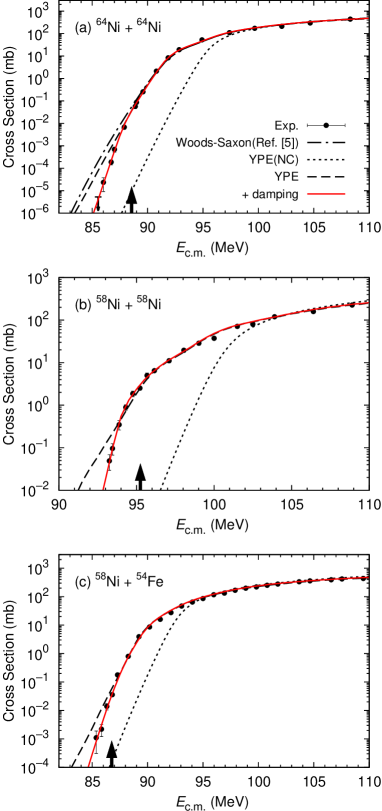
Figure 3: (Color online) Calculated fusion cross sections versus incident energies for the (a) ⁶⁴Ni + ⁶⁴Ni, (b) ⁵⁸Ni + ⁵⁸Ni, and (c) ⁵⁸Ni + ⁵⁴Fe systems. The solid circles denote the experimental data. The solid and dashed lines indicate the calculated results with and without the damping factor, respectively. The dotted lines indicate the calculated results of no coupling. The dash-dotted line indicates the result calculated with the WS potential. The arrows indicate the potential energy at the touching point $V_{\rm Touch}$.

Figure 3 shows the calculated fusion cross sections. The solid and dashed lines indicate the results calculated with and without the damping factor, respectively. The dotted lines indicate the results calculated with no coupling. The experimental data for ⁶⁴Ni + ⁶⁴Ni, ⁵⁸Ni + ⁵⁸Ni, and ⁵⁸Ni + ⁵⁴Fe (solid circles) are taken from Refs. Jiang04 ; Beck81 ; Beck82 ; Stef10 , respectively. In the figure, one can see that drastic improvements have been made by taking into account the damping in the CC form factor, as compared to the results calculated without the damping factor. I tested the dependence of $\hbar\omega_{\rm GS}$ on the calculated results, but it was negligible above the lowest incident energy of the experimental data in each system. Interestingly, in the ⁵⁸Ni + ⁵⁸Ni system, the fusion cross sections are slightly enhanced around an incident energy of 95 MeV due to the damping factor.

For comparison, in Fig. 1 (a), I also plot the result calculated with the WS potential using the parameters given in Ref. Jiang04 . Since the YPE potential is much thicker than the WS potential, as shown in Fig. 2, the result calculated with the YPE potential is slightly suppressed. Although the potential thickness around the Coulomb barrier increases considerably in the YPE potential, one cannot reproduce the fusion cross sections at the deep sub-barrier energies only by changing it. The damping factor plays an important role in reproducing the fusion hindrance behavior.

In each of these systems, $V_{\rm Touch}$ remarkably correlates with the incident threshold energy for fusion hindrance. The values of $V_{\rm Touch}$ are tabulated in Tabel 2 and indicated by the arrows in Fig. 3. In all the systems, one can clearly see that the significant decreases in the fusion cross sections start from $V_{\rm Touch}$. Thus, the threshold rule for the potential energy at the touching point works very well in the medium-heavy mass systems.

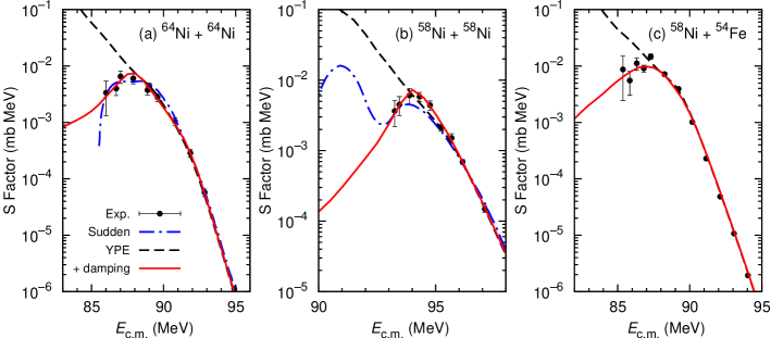
Figure 4: (Color online) Astrophysical S factor representations of the fusion cross sections versus incident energies for the (a) ⁶⁴Ni + ⁶⁴Ni, (b) ⁵⁸Ni + ⁵⁸Ni, and (c) ⁵⁸Ni + ⁵⁴Fe systems. The solid and dashed lines indicate the results calculated with and without the damping factor, respectively. The dash-dotted lines indicate the results calculated with the sudden model from Refs. mis06

Figure 4 shows the astrophysical S factor representations of the fusion cross sections for these systems. I take $\eta_{0}=$ 75.23, 69.99, and 66.0 MeV for the ⁶⁴Ni + ⁶⁴Ni, ⁵⁸Ni + ⁵⁸Ni, and ⁵⁸Ni + ⁵⁴Fe systems, respectively. In the figure, the solid and dashed lines indicate the results calculated with and without the damping factor, respectively. In all the systems, the results calculated with the damping factor are in good agreement with the experimental data. In each of these systems, the calculated result well reproduces the single peak structure of the experimental data. For comparison, the results calculated with the sudden model from Ref. mis06 are plotted by the dash-dotted lines in Figs. 4 (a) and (b). In both the systems, the adiabatic model better reproduces the experimental data compared to the sudden model. The S factors of the adiabatic and sudden models at the deep sub-barrier energies are considerably different from each other, although the reproductions of the fusion cross sections calculated with the two models are similar to an extent.

In the ⁶⁴Ni + ⁶⁴Ni system, the S factor calculated with the sudden model significantly decreases with decreasing incident energy, whereas the adiabatic model has a much weaker and smoother energy dependence. In the ⁵⁸Ni + ⁵⁸Ni system, unphysical fluctuations of the S factor are recognizable at extremely low incident energies in the sudden model, whereas the adiabatic model has a single, smooth peak. Thus, fusion cross section measurements at much deeper incident energies for this system are appropriate for discriminating which model can better describe the deep sub-barrier fusions.

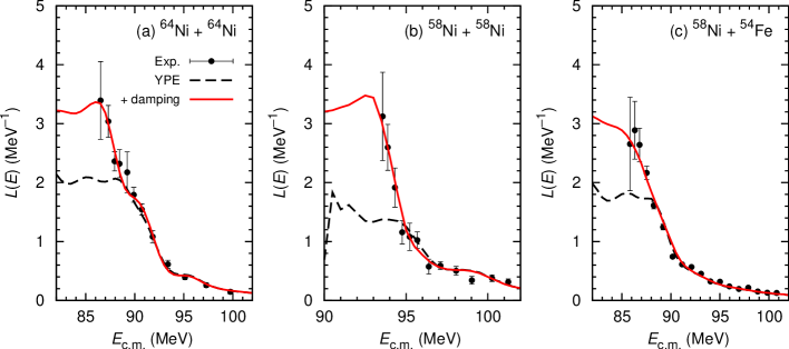
Figure 5: (Color online) Logarithmic derivative representations of the fusion cross sections versus incident energies for the (a) ⁶⁴Ni + ⁶⁴Ni, (b) ⁵⁸Ni + ⁵⁸Ni, and (c) ⁵⁸Ni + ⁵⁴Fe systems. The solid and dashed lines indicate the results calculated with and without the damping factor, respectively.

Figure 5 shows the logarithmic derivative representations of the fusion cross sections versus incident energies. The solid and dashed lines indicate the results calculated with and without the damping factor, respectively. All the calculated results are in good agreement with the experimental data. In each of these systems, the result calculated with the damping factor is saturated below a certain incident energy. Conversely, the result calculated with the sudden model significantly increases or fluctuates with decreasing incident energy mis06 . At the deep sub-barrier energies, the energy dependence of the logarithmic derivative in the adiabatic model is substantially different from that in the sudden model.

III.2 Medium-light mass systems

Table 3: Input parameters for the coupling strengths in the CC calculations for the ⁴⁰Ca + ⁴⁰Ca, ⁴⁸Ca + ⁴⁸Ca, and ²⁴Mg + ³⁰Si systems. All symbols are the same as those in Table 1.

Nucleus	$\lambda^{\pi}$	$E_{\rm ex}$ (MeV)	$\beta_{\lambda}^{\rm Coul}$	$\beta_{\lambda}^{\rm Nucl}$	$N_{\rm ph}$
(a) 40Ca + 40Ca (see Refs. Monta12 ; Esb89 )
40Ca	$2^{+}$	3.905	0.119	0.119	1
	$3^{-}$	3.737	0.402	0.402	1
(b) 48Ca + 48Ca (see Ref. Esb10 )
48Ca	$2^{+}$	3.832	0.102	0.154	2
	$3^{-}$	4.507	0.203	0.154	1
(c) 24Mg + 30Si (see Ref. Jiang14 )
24Mg	$2^{+}$	1.369	0.608	0.460	1
30Si	$2^{+}$	2.235	0.330	0.330	1
	$3^{-}$	5.497	0.275	0.275	1

Table 4: Input parameters for the YPE potential and the damping factor in the ⁴⁰Ca + ⁴⁰Ca, ⁴⁸Ca + ⁴⁸Ca, and ²⁴Mg + ³⁰Si systems. All symbols are the same as those in Tabel 2.

System	$r_{0}$	$a_{0}$	$V_{\rm GS}$	$\hbar\omega_{\rm GS}$	$V_{\rm Touch}$	$r_{d}$	$a_{d}$
	(fm)	(fm)	(MeV)	(MeV)	(MeV)	(fm)	(fm)
40Ca + 40Ca	1.191	0.68	14.2	4.40	47.6	1.240	0.52
48Ca + 48Ca	1.185	0.68	3.0	3.89	43.0	1.280	0.60
24Mg + 30Si	1.190	0.68	$-17.9$	5.39	15.8	1.430	1.25

Next, I discuss the fusion hindrance in the medium-light mass systems for the ⁴⁰Ca + ⁴⁰Ca, ⁴⁸Ca + ⁴⁸Ca, and ²⁴Mg + ³⁰Si systems. These systems are appropriate to check the dependence of the reaction Q value on the fusion hindrance. The reaction Q values of the ⁴⁰Ca + ⁴⁰Ca, ⁴⁸Ca + ⁴⁸Ca, and ²⁴Mg + ³⁰Si systems are $Q=-14.2$, $-3.0$, and 17.9 MeV, respectively. All input parameters for the coupling strengths of the CC calculations are tabulated in Table 3. In the calculations, I included couplings only to the low-lying $2^{+}$ and $3^{-}$ states and all mutual excitations of these states. For ⁴⁰Ca + ⁴⁰Ca, I used the same deformation parameters between $\beta^{\rm Coul}$ and $\beta^{\rm Nucl}$, which differ from those of Ref. Monta12 . All input parameters for the YPE potential and the damping factor are tabulated in Table 4.

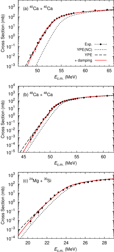
Figure 6: (Color online) Calculated fusion cross section versus incident energies for the (a) ⁴⁰Ca + ⁴⁰Ca, (b) ⁴⁸Ca + ⁴⁸Ca, and (c) ²⁴Mg + ³⁰Si systems. All symbols are the same as those in Fig. 3.

Figure 6 shows the obtained fusion cross sections. All the calculated results (solid lines) are in good agreement with the experimental data (solid circles). The experimental data for the ⁴⁰Ca + ⁴⁰Ca, ⁴⁸Ca + ⁴⁸Ca, and ²⁴Mg + ³⁰Si systems are from Refs. Monta12 , Ref. Stef09 , and Ref. Jiang14 , respectively. In comparison to the medium-heavy mass systems, the effect of the damping factor on the fusion cross sections is relatively small in each system (dashed lines in Fig. 6). This is because that the potential energies at the touching point are lower than the lowest incident energies in the available experimental data ($V_{\rm Touch}$ in Table 4). Thus, the calculated results presented in the energy regions of Fig. 6 are independent of the slope of the one-body potential around the touching point associated with $\hbar\omega_{\rm GS}$. In this regard, it seems that the fusion hindrance is relatively weak in these systems.

The potential energies at the touching point in these system weakly correlate with the threshold incident energies for the fusion hindrance. In each of these systems, the value of $V_{\rm Touch}$ is lower than the threshold incident energy for fusion hindrance by about 3$\sim$5 MeV. In these systems, the deformation parameters in the coupling strengths from the CC calculations are considerably large. This implies the effect of the damping factor starts much before the touching point. Thus, the adiabatic potential in the CC model is affected by these large deformation effects, which is discussed later in Sec. IV-A. In these medium-light mass systems, the threshold rule should be modified by taking into account the deformation effects.

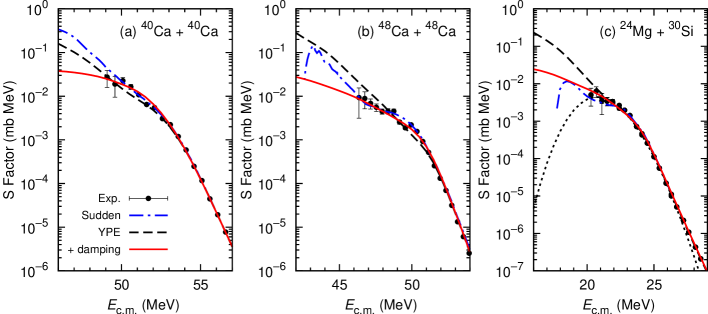
Figure 7: (Color online) Astrophysical S factor representations of the fusion cross sections versus incident energies for the (a) ⁴⁰Ca + ⁴⁰Ca, (b) ⁴⁸Ca + ⁴⁸Ca, and (c) ²⁴Mg + ³⁰Si systems. All symbols are the same as those in Fig. 4. The dotted line indicates the functional form proposed by Jiang et al. Jiang14 .

Figure 7 shows the astrophysical S factor representations of the fusion cross sections versus incident energies for these systems. I take $\eta_{0}=40.8$, 45.5, and 22.0 for the ⁴⁰Ca + ⁴⁰Ca, ⁴⁸Ca + ⁴⁸Ca, and ²⁴Mg + ³⁰Si systems, respectively. All the calculated results (solid lines) are in good agreement with the experimental data (solid circles). For comparison, the S factors calculated with the sudden model taken from Refs. Monta12 ; Esb10 ; Jiang14 are plotted by the dash-dotted lines. The S factors calculated with the damping factor are in good agreement with the experimental data compared to those with the sudden model. As discussed in the medium-heavy mass systems, the S factors calculated with the damping factor have a much smoother energy dependence than those with the sudden model.

In each of these systems, the peak structure in the S factor calculated with the damping factor is not visible, although Jiang et al. assumed it was in their fitting function Jiang14 . For comparison, the S factor proposed by Jiang et al. is plotted by the dotted line in Fig. 7 (c). The S factor of Jiang et al. has a strong energy dependence and peak structure. However, there is no physical reason why the S factor can be described by the functional form proposed by them. This large difference in S factor behavior at the low incident-energy region strongly affects the estimations of astrophysical reaction rates. Nevertheless, a few additional data points with high precision at the low-energy region are necessary to determine this behavior.

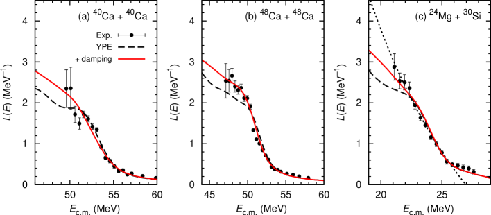
Figure 8: (Color online) Logarithmic derivative representations of the fusion cross sections versus incident energies for the (a) ⁴⁰Ca + ⁴⁰Ca, (b) ⁴⁸Ca + ⁴⁸Ca, and (c) ²⁴Mg + ³⁰Si systems. All symbols are the same as those in Fig. 5.

Figure 8 shows the logarithmic derivative representations of the calculated fusion cross sections for the ⁴⁰Ca + ⁴⁰Ca, ⁴⁸Ca + ⁴⁸Ca, and ²⁴Mg + ³⁰Si systems. The results calculated with the damping factor (solid lines) are in good agreement with the experimental data (solid circles). For comparison, the logarithmic derivative presented by Jiang et al. is also plotted by the dotted line. In each of these systems, the calculated S factor monotonically increases with decreasing incident energy and the slope changes at a certain energy. In contrast, the logarithmic derivative of Jiang et al. linearly increases with decreasing incident energy.

In the adiabatic model presented in this paper, the reaction Q value is an important input parameter in the heavy ion-ion potential for estimating the ground-state energy of the compound system. In these systems, the compound state energies are sufficiently lower than the potential energies at the touching point (Table 4). Therefore, the dependence of the Q values on the fusion cross sections is negligible in the adiabatic model, although Jiang discussed the effect of the positive Q value on the fusion hindrance Jiang14 .

III.3 Mass-asymmetric reaction systems

Table 5: Input parameters for the coupling strengths in the CC calculations for the ⁴⁸Ca + ⁹⁶Zr and ¹⁶O + ²⁰⁸Pb systems. All symbols are the same as those in Table. 1.

Nucleus	$\lambda^{\pi}$	$E_{\rm ex}$ (MeV)	$\beta_{\lambda}^{\rm Coul}$	$\beta_{\lambda}^{\rm Nucl}$	$N_{\rm ph}$
(a) 48Ca + 96Zr (see Refs. Esb09 )
48Ca	$2^{+}$	3.832	0.102	0.126	2
96Zr	$2^{+}$	1.751	0.079	0.079	1
	$3^{-}$	1.897	0.295	0.295	3
(b) 16O + 208Pb (see Refs. Esb07 )
16O	$3^{-}$	6.129	0.713	0.713	2
208Pb	$3^{-}$	2.615	0.111	0.111	2

Table 6: Input parameters for the YPE potential and the damping factor in the ⁴⁸Ca + ⁹⁶Zr and ¹⁶O + ²⁰⁸Pb systems. All symbols are the same as those in Table. 2

System	$r_{0}$	$a_{0}$	$V_{\rm GS}$	$\hbar\omega_{\rm GS}$	$V_{\rm Touch}$	$r_{d}$	$a_{d}$
	(fm)	(fm)	(MeV)	(MeV)	(MeV)	(fm)	(fm)
48Ca + 96Zr	1.198	0.68	45.9	3.16	88.8	1.30	1.05
16O + 208Pb	1.20	0.68	46.5	3.33	70.5	1.255	1.14

Finally, I discuss the mass-asymmetric reaction system for the ⁴⁸Ca + ⁹⁶Zr and ¹⁶O + ²⁰⁸Pb systems. All input parameters for the coupling strengths in the CC calculations are tabulated in Table. 5. In the calculations, I included couplings only to the low-lying $2+$ and $3^{-}$ states and all mutual excitations of these states. For ¹⁶O + ²⁰⁸Pb, I included only the $3^{-}$ states of ¹⁶O and ²⁰⁸Pb and used the same deformation parameters of $\beta^{\rm Coul}$ and $\beta^{\rm Nucl}$, although those of Ref. Esb07 are different.

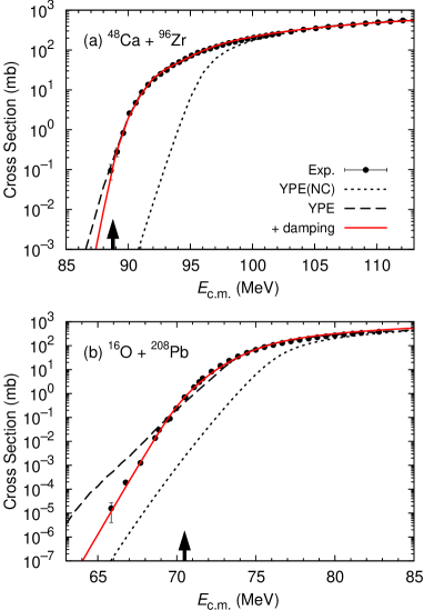
Figure 9: (Color online) Calculated fusion cross sections versus incident energies for the (a) ⁴⁸Ca + ⁹⁶Zr and (b) ¹⁶O + ²⁰⁸Pb systems. All symbols are the same as those in Fig. 3.

Figure 9 shows the calculated fusion cross sections versus incident energies. The results calculated with the damping factor (solid lines) are in good agreement with the experimental data (solid circles). The experimental data for ⁴⁸Ca + ⁹⁶Zr and ¹⁶O + ²⁰⁸Pb is from Ref. Stef06 and Refs. das07 ; Morton99 , respectively. In the ¹⁶O + ²⁰⁸Pb system, it is seen that a drastic improvement has been made by taking into account the damping factor in the CC form factor, as compared to the result without the damping factor (dashed line). A strong fusion hindrance can be seen in the ¹⁶O + ²⁰⁸Pb system.

In these systems, the potential energies at the touching point strongly correlate with the threshold incident energies for fusion hindrance. The values of $V_{\rm Touch}$ are tabulated in Table. 6 and are indicated by the solid arrows in Fig. 9. The threshold rule works well in these systems. The experimental data for the ¹⁶O + ²⁰⁸Pb system are most adequate for discussing the fusion hindrance, because the lowest incident energy in the experimental data is lower than $V_{\rm Touch}$ by about 5 MeV. Only this measurement has achieved such deep sub-barrier energy. This is because that the position of $V_{\rm Touch}$ approaches that of the Coulomb barrier as the mass number of the compound system increases. Thus, the fusion hindrance would be more clearly observed in such heavy-mass compound system. The fusion hindrance phenomena would play a decisive role in the formation of super heavy elements.

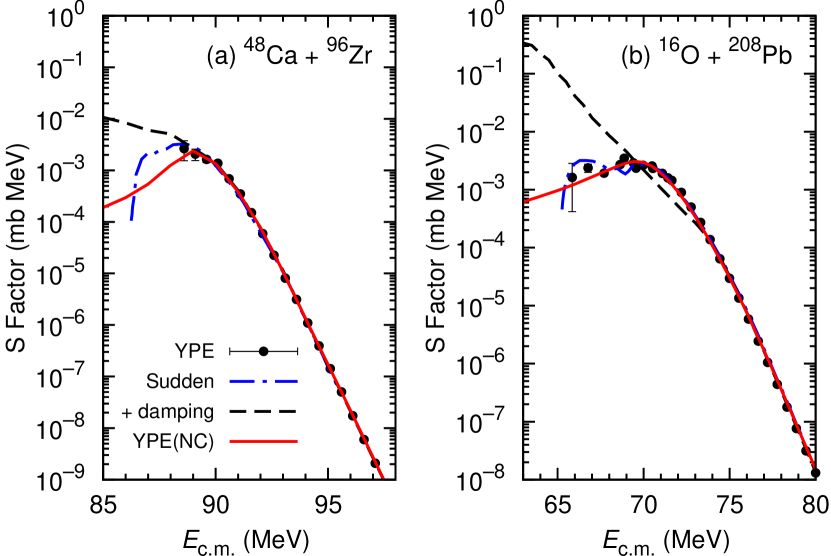
Figure 10: (Color online) Astrophysical S factor representation of the fusion cross section versus incident energies for the (a) ⁴⁸Ca + ⁹⁶Zr and (b) ¹⁶O + ²⁰⁸Pb systems. All symbols are the same as those in Fig. 4

Figure 10 shows the astrophysical S factor representations of the fusion cross sections for the ⁴⁸Ca + ⁹⁶Zr and ¹⁶O + ²⁰⁸Pb systems. I take $\eta_{0}=77.0$ and 49.0 for the ⁴⁸Ca + ⁹⁶Zr and ¹⁶O + ²⁰⁸Pb systems, respectively. The results calculated with the damping factor (solid lines) are in good agreement with the experimental data (solid circles). For comparison, the result calculated with the sudden model taken from Ref. Esb10 is plotted by the dash-dotted line in Fig. 10 (b). In the sudden model, the S factor is suddenly cut off around 66 MeV corresponding to the bottom of the shallow potential pocket. Alternatively, at low incident energies, the S factor calculated with the adiabatic model linearly decreases with decreasing incident energy. The result calculated with the adiabatic model has a much smoother and weaker energy dependence than that with the sudden model.

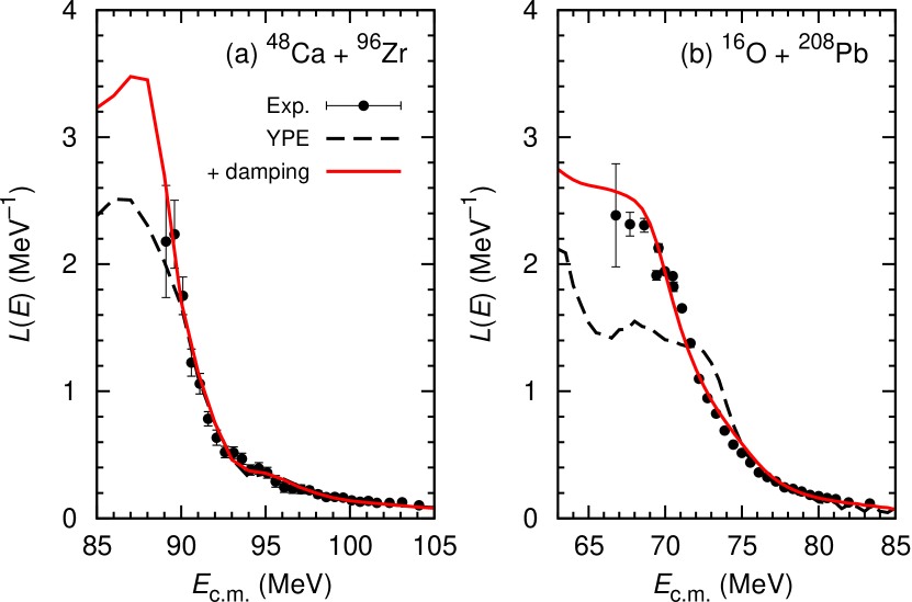
Figure 11: (Color online) Logarithmic derivative representations of the fusion cross sections versus incident energies for the (a) ⁴⁸Ca + ⁹⁶Zr and (b) ¹⁶O + ²⁰⁸Pb systems. All symbols are the same as those in Fig. 5.

Figure 11 shows the logarithmic derivative representations of the fusion cross sections versus incident energies for the ⁴⁸Ca + ⁹⁶Zr and ¹⁶O + ²⁰⁸Pb systems. The results calculated with the damping factor (solid lines) are in good agreement with the experimental data (solid circles). In these systems, the results calculated with the adiabatic model are saturated at extremely low incident energies. Conversely, the results calculated with the sudden model may significantly increase with decreasing incident energy, as shown in Ref. mis06 .

I also calculated the fusion cross section for the ¹²C + ¹⁹⁸Pt system where the fusion hindrance was recently observed Arad15 . The result calculated with the damping factor well reproduces the experimental data of the fusion cross section and its S factor and logarithmic derivative representations. The potential energy at the touching point also strongly correlates with the incident threshold energy for fusion hindrance.

IV Discussion

IV.1 Adiabatic potential

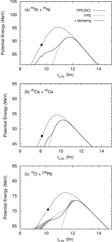
Figure 12: Adiabatic potentials in CC calculations versus the center-of-mass distance of colliding nuclei for the (a) ⁶⁴Ni + ⁶⁴Ni, (b) ⁴⁰Ca + ⁴⁰Ca, and (c) ¹⁶O + ²⁰⁸Pb systems. The solid and dotted lines indicate the results calculated with and without the damping factor, respectively. The dashed lines indicate the results calculated with no couplings. The solid circles denote the energies at the touching point. The gray area in (c) represents the adiabatic potential extracted from the potential inversion method Hagino07 .

I discuss here the adiabatic potential, namely, the lowest eigenvalue obtained by diagonalizing the coupling matrix elements in the CC model at each center-of-mass distance Hagino07 . Figure 12 shows the adiabatic potential obtained for the (a) ⁶⁴Ni + ⁶⁴Ni, (b) ⁴⁰Ca + ⁴⁰Ca, and (c) ¹⁶O + ²⁰⁸Pb systems. The solid and dotted lines indicate the adiabatic potentials calculated with and without the damping factor, respectively.

In each of these figures, one can see that the adiabatic potential calculated with the damping factor (solid line) becomes thicker than that without the damping factor (dotted line) below the potential energy at the touching point indicated by the solid circle. This is the main effect of the damping factor on the fusion hindrance behavior. In the adiabatic model, the adiabatic potential becomes thicker below the potential energy at the touching point and this increase in thickness naturally accounts for the fusion hindrance behavior.

In Fig. 12 (b), it seems that the increase in the thickness of the adiabatic potential is relatively small compared to the other heavy-mass compound systems. In fact, the fusion hindrance behavior of the fusion cross sections obtained with the adiabatic model is small in the medium-light mass system. This is associated with coupling strengths causing the enhancements in the fusion cross sections. In this system, the difference between the thicknesses of the bare potential (dashed line) and the adiabatic potential without the damping factor (dotted line) is small, indicating that the coupling strengths in this system are weak compared to those of heavier compound mass systems. Thus, the increase in the thickness of the adiabatic potential due to the damping factor also becomes small. As a result, the fusion hindrance behavior is relatively small in the medium-light mass systems.

In Fig. 12 (c), the adiabatic potential extracted with the potential inversion method Hagino07 from the experimental data is illustrated by the gray area. Clearly, the adiabatic potential calculated with the damping factor strongly correlates with that of the potential inversion method. This is strong evidence for the presence of the smooth transition from sudden to adiabatic processes and the coordinate-dependent coupling strength.

IV.2 Barrier Distribution

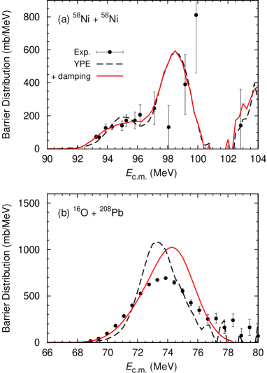
Figure 13: (Color online) Barrier distribution versus incident energies for the (a) ⁵⁸Ni + ⁵⁸Ni and (b) ¹⁶O + ²⁰⁸Pb systems. The solid and open circles denote the experimental data. The solid and dashed lines indicate the calculated results with and without the damping factor, respectively.

For the ⁵⁸Ni + ⁵⁸Ni and ¹⁶O + ²⁰⁸Pb systems, a large improvement in the barrier distribution $D_{\rm fus}(E)=d^{2}(E\sigma_{\rm fus})/dE^{2}$ has been achieved by taking into account the damping factor. Figure 13 shows the barrier distributions versus incident energies for the (a) ⁵⁸Ni + ⁵⁸Ni and (b) ¹⁶O + ²⁰⁸Pb systems.

In Fig. 13 (a), one can see a small peak of the barrier distribution calculated without the damping factor (dashed line) around $E_{\rm c.m.}=95$ MeV. By taking into account the damping factor, this peak structure vanishes, and the plateau structure appears between about 94-97 MeV (solid line). This plateau structure is in good agreement with the experimental data (solid circles). The experimental data for this system is adequate for investigating the properties of the fusion hindrance, because a clear signature of the fusion hindrance appears in the barrier distribution of the fusion cross sections around $10^{-1}\sim 1$ mb. In addition, the strong fusion hindrance can be seen for this system in the calculated result of the fusion cross section after implementing the damping factor. However, the accuracy of the experimental data is still insufficient to determine the energy dependence of the calculated barrier distribution. Thus, in this system, much higher precision fusion data around these incident energies are required to study the fusion hindrance properties in details.

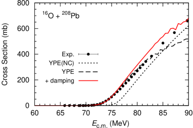
Figure 14: (Color online) Fusion cross section versus incident energies for the ¹⁶O + ²⁰⁸Pb system. The solid circles denote the experimental data. The solid and dashed lines indicate the results calculated with and without the damping factor, respectively. The dotted line indicates the calculated result with no couplings.

For the ¹⁶O + ²⁰⁸Pb system, the agreement between the tails of the experimental data and the result calculated with the damping factor in the low incident-energy region is greatly improved [solid and dashed lines in Fig. 13 (b)]. The peak position of the result calculated with the damping factor shifts to the higher incident energy by about 2 MeV, compared to that without the damping factor. The calculated barrier distribution at the peak position is also reduced by taking into account the damping factor. However, it seems that the width of the barrier distribution calculated with the damping factor becomes wider than that without the damping factor. In fact, for this system, fusion cross sections at incident energies highly above the Coulomb barrier are overestimated when the damping factor is employed (solid line in Fig. 14). In this system, other dissipative mechanisms, including single particle excitations, as discussed in Refs. Yusa10 ; Yusa13 , are necessary to reproduce the fusion cross sections at incident energies highly above the Coulomb barrier. The YPE potential, which is optimized in the adiabatic process, may be also inapplicable to this high incident-energy region. Note that in the systems except for the mass-asymmetric ¹⁶O + ²⁰⁸Pb and ¹²C + ¹⁹⁸Pt systems, the calculated fusion cross sections with the adiabatic model are in good agreement with the experimental data even above the Coulomb barrier.

IV.3 Average angular momentum of compound nucleus

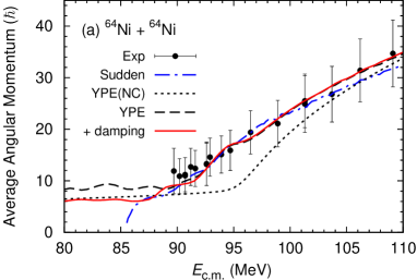
Figure 15: (Color online) Average angular momentum of compound nucleus versus incident energies for the ⁶⁴Ni + ⁶⁴Ni system. The sold circles denote the experimental data from Ref. Ack96 . The solid and dashed lines indicate the calculated results with and without the damping factor, respectively. The dotted lines indicate the CC calculation with no couplings. The dash-dotted line indicates the result calculated with the sudden model taken from Ref. mis06 .

Figure 16: Partial fusion cross section versus angular momentum $I$ at an incident energy of 87 MeV for the ⁶⁴Ni + ⁶⁴Ni system. The solid line with solid circles and the dashed line with open circles indicate the results calculated with and without the damping factor, respectively.

An important piece of experimental data for discriminating between the adiabatic and sudden models is the average angular momentum of a compound nucleus at extremely low incident energies. Figure 12 shows the average angular momentum of the compound nucleus versus incident energies for the ⁶⁴Ni + ⁶⁴Ni system. The experimental data for the ⁶⁴Ni + ⁶⁴Ni is from Ref. Ack96 , denoted by the solid circles. The solid and dashed lines indicate the results calculated with and without the damping factor, respectively. In the ⁶⁴Ni + ⁶⁴Ni system, the result calculated with the damping factor decreases with decreasing incident energy. Below the potential energy at the touching point ($V_{\rm Touch}=88.6$ MeV), the result calculated with the damping factor remains constant at around 8 $\hbar$. Subsequently, the result calculated with the damping factor is lower than that without the damping factor by about 20%. For the ¹²C + ¹⁹⁸Pt system, the result calculated with the damping factor is in good agreement with the experimental data of overall incident energy Arad15 .

Figure 16 shows the calculated partial cross sections versus the angular momentum $I$ at an incident energy of 85 MeV for the ⁶⁴Ni + ⁶⁴Ni system. The solid line with solid circles and the dashed line with open circles indicate the results calculated with and without the damping factor, respectively. In the figure, in the adiabatic model, the partial cross section at each $I$ is naturally reduced by the effects of the damping factor. On the other hand, the average angular momentum calculated with the sudden model is strongly suppressed at energies below the threshold energy [dash-dotted line in Fig. 15 (a)]. This result indicates that a mechanism of the fusion hindrance in the sudden model would be the cutoff of high angular-momentum components in the partial cross sections due to the shallow potential pocket. In this respect, a compound nucleus formed at the deep sub-barrier incident energy in the sudden model has substantially low angular momentum. Subsequently, particle evaporation from the compound state would be forbidden, because the angular momentum necessary for particle evaporation is insufficient. Therefore, the properties of the formed compound nucleus are considerably different between the adiabatic and sudden models. Thus, in order to discriminate the two models, it is also important to measure the average angular momentum at deep sub-barrier energies.

IV.4 Systematic trends of the radius and diffuseness parameters in the damping factor

Figure 17: Systematic trends of the (a) radius and (b) diffuseness parameters in the damping factor versus the mass numbers of the compound nuclei for the systems presented in this paper. The solid circles denote the obtained values fitted to the experimental data. The dashed lines indicate the average value of all the obtained values in individual radius and diffuseness parameters.

Next, I test the systematic trends of the obtained radius and diffuseness parameters in the damping factor for the systems presented in this paper. Figure 17 shows the (a) radius and (b) diffuseness parameters versus the mass numbers of the compound nuclei for the systems presented in this paper. In the figure, the solid circles denote the obtained values. The dashed line indicates the average value for all the obtained values of the individual radius and diffuseness parameters. Clearly, the values of $r_{d}$ are almost constant at around an average value of 1.31 fm. Except for a few points, the values of $a_{d}$ are also distributed around an average value of 1.02 fm.

As shown in Refs. ich13 ; ich15 , the damping factor strongly correlates with the damping of the transition strength of individual colliding nuclei when they approach one another. In this respect, the damping of the transition strengths would start at the overlapping between the tails of the density distributions for colliding nuclei. That is, the radius parameter of the damping factor would correlate with a range of interactions between the colliding nuclei. This would result in an almost constant value of $r_{d}$ in all the systems. Alternatively, $a_{d}$ is associated with the damping strength of quantum vibrations, which would strongly depend on an inner nuclear structure of individual colliding nuclei. In fact, the values of $a_{d}$ for the ⁴⁰Ca + ⁴⁰Ca and ⁴⁸Ca + ⁴⁸Ca systems, where ^40,48Ca have the strong shell effects, which largely deviate from the average value. In this sense, the values of $a_{d}$ would be somewhat scattered around the average value.

IV.5 Correlation between $V_{\rm Touch}$ and the incident threshold energy for fusion hindrance

As shown in Sec. III, the potential energies at the touching point $V_{\rm Touch}$ strongly correlate with the incident threshold energies for fusion hindrance in the medium-heavy mass and mass-asymmetric reaction systems (see the arrows in Figs. 3 and 9). In the medium-light mass systems, the correlation is relatively weak. This would result from considerably larger deformation parameters associated with coupling strengths in these systems compared to those in the other systems. In addition, the curvature of the bare potentials around the Coulomb barrier is relatively large [Fig. 12 (b)]. Thus, the effect of the damping factor starts much before the touching point in this system. In this regards, the threshold rule should be modified considering the deformation parameter effects in this system. This modification is now in progress.

V Summary

In summary, I have proposed a novel extension of the standard CC model to describe the fusion hindrance phenomenon observed at extremely low incident energies. I have systematically investigated various deep sub-barrier fusion reactions using an adiabatic approach.

A key quantity for understanding fusion hindrance is the potential energy at the touching point $V_{\rm Touch}$. The threshold incident energies for fusion hindrance strongly correlate with $V_{\rm Touch}$. At incident energies below $V_{\rm Touch}$, the inner turning point of the potential energy becomes inside the touching point. That is, a composite system must penetrate through a residual Coulomb potential with an overlapping configuration before fusion occurs. Thus, the dynamics in the overlapping region of the two colliding nuclei would be responsible for the fusion hindrance.

I have described the fusion hindrance based on an adiabatic approach. In the adiabatic approach, fusion is assumed to occur slowly, and neck formation occurs in the overlapping region. The nuclear density distributions then evolve with the lowest-energy configuration. Based on this picture, one can calculate the one-body potential energy with an appropriate adiabatic model. However, one cannot directly apply the obtained one-body potential to a standard CC model, because of double counting of CC effects.

To avoid this double counting, an important extension of the standard CC model is the introduction of a damping factor in the coupling form factor, which enables a smooth transition from sudden to adiabatic processes. Namely, the damping factor represents the damping of quantum vibrations and suppresses transitions between reaction channels when two colliding nuclei approach one another. By introducing the damping factor in the coupling form factor, one can correctly estimate the tunneling probability in the one-body region, when an appropriate one-body potential is taken into account in the bare heavy ion-ion potential in the CC model.

In this paper, I adopted the YPE model as a basic heavy ion-ion potential. An advantage of this potential model is a unified description of both the two- and one-body systems. For the purpose of systematic investigations, in this paper, the one-body potential is approximated with a third-order polynomial function. This procedure works very well, because the lowest incident energies in the experiments, which have been performed until now, are lower than the potential energies at the touching point only by a few MeV.

Based on this framework, I have systematically calculated the medium-heavy mass systems of ⁶⁴Ni + ⁶⁴Ni, ⁵⁸Ni + ⁵⁸Ni, and ⁵⁸Ni + ⁵⁴Fe, the medium-light mass systems of ⁴⁰Ca + ⁴⁰Ca, ⁴⁸Ca + ⁴⁸Ca, and ²⁴Mg + ³⁰Si, and the mass-asymmetric systems of ⁴⁸Ca + ⁹⁶Zr, ¹²C + ¹⁹⁸Pt, and ¹⁶O + ²⁰⁸Pb. In addition, I have calculated their fusion cross sections, the astrophysical S factor and the logarithmic derivative representations of those. In all the systems, the calculated results are in excellent agreement with the experimental data, indicating that the smooth transition from sudden to adiabatic processes occurs in the deep sub-barrier fusion reactions, and the coordinate-dependent coupling strength is responsible for the fusion hindrance.

I have also showed the adiabatic potential, which is the lowest eigenvalue obtained by diagonalizing the coupling matrix elements, in the CC model for the ⁶⁴Ni + ⁶⁴Ni, ⁴⁰Ca + ⁴⁰Ca, and ¹⁶O + ²⁰⁸Pb systems. Because of the introduction of the damping factor, the adiabatic potential using the damping factor becomes much thicker than without the damping factor. This naturally accounts for the fusion hindrance behavior. The adiabatic potential for the ¹⁶O + ²⁰⁸Pb systems is in good agreement with that extracted from the potential inversion method. For the ⁵⁸Ni + ⁵⁸Ni and ¹⁶O + ²⁰⁸Pb systems, large improvements in the barrier distribution at low incident energies were made by taking into account the damping factor.

The adiabatic and sudden models significantly differ in the calculated average angular momentum of the compound nuclei. The average angular momentum estimated with the adiabatic model is saturated below the threshold incident energy. Conversely, that with the sudden model is strongly suppressed at low incident energies, because a mechanism of the fusion hindrance in the sudden model is the cutoff of high angular-momentum components in the partial waves due to the shallow potential pocket.

The obtained parameters of individual $r_{d}$ and $a_{d}$ in the damping factor are nearly constant in all the systems. The values of $a_{d}$ are somewhat scattered around its average value, because $a_{d}$ would depend on the shell structure of the composite system. The strong correlation between $V_{\rm Touch}$ and the threshold incident energy for the fusion hindrance can be seen in the medium-heavy mass and mass-asymmetric systems. For the medium-light mass system, this correlation is somewhat weak, because the deformation parameters associated with the coupling strengths in this system are large compared to those at heavier compound mass systems. It is necessary to modify the threshold rule with the effects of the deformation parameters in the medium-light mass systems.

Appendix A Lemniscatoids parametrization

Figure 18: Shapes described using the lemniscatoids parametrization from $s=0$ to 1 with an increment of 0.25. The mass asymmetry $\alpha$ of the shape corresponds to the ¹⁶O + ²⁰⁸Pb system.

The lemniscatoids parametrization proposed by Royer Roy82 ; Roy84 ; Roy85 is a special case of the Cassinian oval. This parametrization allows us to smoothly describe from the touching configuration of two spheres to a single spherical shape as functions of the elongation parameter $s$ and the mass-asymmetry parameter $\alpha$. The described shape has a single sphere at $s=0$ and the touching configuration of two spheres at $s=1$. The mass-asymmetry parameter is defined as $\alpha=(A_{1}-A_{2})/(A_{1}+A_{2})$, where $A_{1}$ and $A_{2}$ are the total mass numbers of the fragments 1 and 2. The radius of the spherical composite system is given by $R_{0}=r_{0}(A_{1}+A_{2})^{1/3}$, where $r_{0}$ is the radius parameter.

In the cylindrical coordinate system, the radial $\rho$ and $z$ coordinates are expressed as the dimensionless parameters $\varrho=\rho/R_{0}$ and $\zeta=z/R_{0}$. The radial displacement of the shapes described with the lemniscatoids parametrization for the fragments 1 and 2 is given by

$$\varrho_{i}^{2}(\zeta)=\begin{cases}\displaystyle\frac{1}{2}\left(A^{2}-2\zeta_{c}^{2}+\sqrt{A^{4}+4(C_{i}^{2}-A^{2})\zeta_{c}^{2}}\right)&(A\neq 0)\\[16.0pt] C_{i}|\zeta_{c}|-\zeta_{c}^{2}&(A=0),\end{cases}$$ (17)

where $\zeta_{c}=\zeta-\zeta_{g}$, $\zeta_{g}$ is the constant to shift the center-of-mass position of the whole system to the origin, $A$ is the neck diameter parameter, and $C_{i}$ are the radius parameter of individual fragments 1 and 2. The index $i$ stands for fragments 1 and 2. The parameters $A$ and $C_{i}$ are determined by the condition of the volume conservation. The regions of $z$ for the fragments 1 and 2 are given by $-C_{1}+\zeta_{g}\leq\zeta\leq\zeta_{g}$ and $\zeta_{g}\leq\zeta\leq C_{2}+\zeta_{g}$, respectively.

Here, the parameter $S_{i}$ are defined as $S_{i}=A/C_{i}$. For $\alpha>0$, Royer assumed the $s$ dependence of $S_{i}$ as $S_{1}=s$ and $S_{2}=S_{1}/f_{s}$ Roy84 ; Roy85 , where

$$f_{s}=\sqrt{s^{2}+(1-s^{2})\left(\frac{1-\alpha}{1+\alpha}\right)^{2/3}}.$$ (18)

From this definition, one also obtains $C_{2}=f_{s}C_{1}$. The volume of each fragment $V_{i}$ is given by $V_{i}/R_{0}^{3}=C_{i}^{3}v_{i}$, where

$$v_{i} =\frac{\pi}{2}\left(S_{i}^{2}-\frac{2}{3}+\int_{0}^{1}\sqrt{4(1-S_{i}^{2})\zeta^{2}+S_{i}^{4}}d\zeta\right)$$ (19)

$$=\frac{\pi}{24}\left(4+6S_{i}^{2}+\frac{3S_{i}^{4}}{\sqrt{1-S_{i}^{2}}}\text{Arcsinh}\left(2\frac{\sqrt{1-S_{i}^{2}}}{S_{i}^{2}}\right)\right).$$ (20)

For practical calculations, Eq. (A3) and the numerical integration for its last term are conveniently used to avoid the divergence of Eq. (A4) at $S_{i}=0$ and $1$. The total volume $V$ is given by $V/R_{0}^{3}=V_{1}/R_{0}^{3}+V_{2}/R_{0}^{3}=C_{1}^{3}v_{1}+C_{2}^{3}v_{2}$. With $C_{2}=f_{s}C_{1}$, one obtains $V/R_{0}^{3}=C_{1}^{3}(v_{1}+f_{s}^{3}v_{2})$. Since $V=\frac{4}{3}\pi R_{0}^{3}$, $C_{1}$ is given by

$$C_{1}^{3}=\frac{4}{3}\pi\frac{1}{v_{1}+f_{s}^{3}v_{2}}.$$ (21)

Then, $A$ and $C_{2}$ are calculated by $A=S_{1}C_{1}$ and $C_{2}=f_{s}C_{1}$. For $\alpha<0$, take $S_{1}=S_{2}/f_{s}$ and $S_{2}=s$ with $|\alpha|$ and exchange the indexes 1 and 2 in the above equations.

Next, I calculate $\zeta_{g}$ and the center-of-mass distance $r$ between the fragments 1 and 2. With $\zeta_{g}=0$ in Eq. (A1), $\zeta_{g}$ is given by

$$\zeta_{g}=-\frac{3}{4}\left(\int_{-C_{1}}^{0}\zeta\varrho_{1}^{2}(\zeta)d\zeta+\int_{0}^{C_{2}}\zeta\varrho_{2}^{2}(\zeta)d\zeta\right).$$ (22)

Again with $\zeta_{g}=0$ in Eq. (A1), $r$ is given by

$$\frac{r}{R_{0}}=\frac{\pi}{C_{2}^{3}v_{2}}\int_{0}^{C_{2}}\zeta\varrho_{2}^{2}(\zeta)d\zeta-\frac{\pi}{C_{1}^{3}v_{1}}\int_{-C_{1}}^{0}\zeta\varrho_{1}^{2}(\zeta)d\zeta.$$ (23)

Figure 18 shows the shapes described using the lemniscatoids parametrization from $s=0$ to 1 with an increment of 0.25. The mass asymmetry corresponds to the ¹⁶O + ²⁰⁸Pb system. From the figure, a smooth transition can be seen from the single spherical shape to where the two spherical shapes touch.

The first and second derivatives of Eq. (A1) are necessary for calculating Eq. (13). The first derivative is given by

$$\frac{d\varrho_{i}^{2}(\zeta)}{d\zeta}=\begin{cases}\displaystyle-2\zeta_{c}\left(\frac{2(\varrho_{i}^{2}+\zeta_{c}^{2})-C_{i}^{2}}{2(\varrho_{i}^{2}+\zeta_{c}^{2})-A^{2}}\right)&(A\neq 0)\\[16.0pt] \text{sign}(\zeta_{c})C_{i}-2\zeta_{c}&(A=0).\end{cases}$$ (24)

The second derivative is given by

$$\frac{d^{2}\varrho_{i}^{2}(\zeta)}{d\zeta^{2}}=\begin{cases}\displaystyle\frac{-2}{2(\varrho_{i}^{2}+\zeta_{c}^{2})-A^{2}}\left(2(\varrho_{i}^{2}+\zeta_{c}^{2})-C_{i}^{2}+\left(\frac{d\varrho_{i}^{2}}{d\zeta}+2\zeta_{c}\right)^{2}\right)&(A\neq 0)\\[16.0pt] -2&(A=0).\end{cases}$$ (25)

Appendix B Approximation of the one-body potential energy

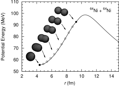
Figure 19: Comparison between the approximation with a third-order polynomial function and the liquid drop energies calculated with the lemniscatoids parametrization. The solid curve indicates the calculated result of the approximation. The open circles denote the liquid drop energies with the lemniscatoids parametrization. Some of nuclear shapes described with the lemniscatoids parametrization are displayed.

Here I describe how to construct the adiabatic one-body potential used in this paper. For simplicity, I approximate the one-body potential energy with a third-order polynomial function based on the YPE model for the purpose of systematic investigations. Thus, the one-body nuclear potential energy $V_{\rm 1bd}^{(N)}$ is given by

$$V_{\rm 1bd}^{(N)}(r)=C_{0}+C_{1}r+C_{2}r^{2}+C_{3}r^{3},$$ (26)

where $C_{n}$ are coefficients determined by the condition that $V_{\rm 1bd}^{(N)}$ is smoothly jointed to the two-body nuclear potential, $V_{\rm 2bd}^{(N)}$, at the touching point, $r_{\rm T}$. I impose that the values of $V_{\rm 1bd}$ and $V_{\rm 2bd}$ and the first derivatives of those are smoothly jointed at the touching point. To determine $C_{n}$, I also assume the position of the compound state $r_{\rm GS}$, the energy of the compound state $E_{\rm GS}$, and the curvature of the potential energy at the compound state $\hbar\omega_{\rm GS}$. The curvature $\hbar\omega_{\rm GS}$ corresponds to the parabolic approximation of the potential energy at the compound state given by $V_{\rm 1bd}\simeq\frac{1}{2}\mu\omega_{\rm GS}^{2}r^{2}$ $(r\sim r_{\rm GS})$, where $\mu$ is the reduced mass of the reaction system. For the Coulomb potential, I use the point charge approximation given by $V_{\rm 1bd}^{(C)}(r)=Z_{T}Z_{P}e^{2}/r$. These conditions are expressed in the following matrix form:

$$\begin{pmatrix}1&r_{\rm T}&r_{\rm T}^{2}&r_{\rm T}^{3}\\ 0&1&2r_{\rm T}&3r_{\rm T}^{2}\\ 1&r_{\rm GS}&r_{\rm GS}^{2}&r_{\rm GS}^{3}\\ 0&0&2&6r_{\rm GS}\end{pmatrix}\begin{pmatrix}C_{0}\\ C_{1}\\ C_{2}\\ C_{3}\end{pmatrix}=\begin{pmatrix}V_{\rm 2bd}^{(N)}(r_{\rm T})\\ {V_{\rm 2bd}^{(N)}}^{\prime}(r_{\rm T})\\ E_{\rm GS}-V_{\rm 1bd}^{(c)}(r_{\rm GS})\\ \mu\omega_{\rm GS}^{2}-{V_{\rm 1bd}^{(c)}}^{\prime\prime}(r_{\rm GS})\end{pmatrix}.$$ (27)

I numerically solve these linear equations and obtain the values of $C_{n}$.

To verify the performance of this procedure, I calculate the liquid-drop energy with Eq. (13) using the lemniscatoids parametrization which describes appropriate neck formations Roy82 ; Roy84 in the ⁶⁴Ni + ⁶⁴Ni system and compare the approximation of the third-order polynomial function with those. In this parametrization, nuclear shapes are described as a function of the center-of-mass distance between two halves of the composite system (Appendix A). To obtain the potential energy, I subtract the self-volume energies of the two colliding nuclei from the total liquid drop energy. In this calculation, I use $r_{0}=1.16$ fm and $a=0.68$ fm. The Coulomb volume energy is also calculated with shape configurations given by the lemniscatoids parametrization. In the procedure described above, the three input parameters $E_{\rm GS}$, $r_{\rm GS}$, and $\hbar\omega_{\rm GS}$ are estimated from the liquid drop energy calculated with the lemniscatoids parametrization. These are taken as $E_{\rm GS}=55.60$ MeV, $r_{\rm GS}=4.38$ fm, and $\hbar\omega_{\rm GS}=3.00$ MeV.

Figure 20: The values of $\hbar\omega_{\rm GS}$ calculated with the liquid-drop model using the lemniscatoids parametrization versus $x=A_{T}^{1/3}\cdot A_{P}^{1/3}$ for various systems. The solid circles denote the calculated results. The solid curve represents a curve fitted to the calculated results.

Figure 19 shows the calculated result of the approximation with the third-order polynomial function (solid lines) and the the liquid drop energy calculated with the lemniscatoids parametrization (open circles). In the figure, the solid circle and square denote the potential energy at the touching point and the energy of the compound state calculated with the liquid drop model, respectively. Some nuclear shapes described with the lemniscatoids parametrization are displayed in the figure. In the figure, the solid curve is clearly in good agreement with the open circles, indicating that the approximation performs very well.

In the procedure described above, there are the three input parameters $E_{\rm GS}$, $r_{\rm GS}$, and $\hbar\omega_{\rm GS}$. In this paper, I estimate the value of $E_{\rm GS}$ from the energy of the compound state calculated with experimental nuclear masses, taken from the AME2003 table audi03 . The value of $r_{\rm GS}$ is calculated with the lemniscatoids parametrization. In this parametrization, the compound state always exhibits a spherical configuration. Thus, $r_{\rm GS}$ is defined as the center-of-mass distance between two halves of the spherical nucleus. This is given by $r_{\rm GS}=3/4\cdot R_{c}$, where $R_{c}$ denotes the nuclear radius of the compound state with $R_{c}=r_{0}(A_{T}+A_{P})^{1/3}$.

The value of $\hbar\omega_{\rm GS}$ is estimated from a fitting curve obtained by systematically investigating the liquid drop energy using the lemniscatoids parametrization (Appendix A). I calculate $V_{\rm 1bd}^{\prime\prime}$ at the compound state using the liquid drop model with the lemniscatoids parametrization for the reaction systems shown in Ref. Jiang06 . I also calculate those for some cold fusion reactions with the ²⁰⁸Pb target. Figure 20 shows the calculated values of $\hbar\omega_{\rm GS}$ as a function of $x=A_{T}^{1/3}\cdot A_{P}^{1/3}$. In the figure, a strong correlation between $\hbar\omega_{\rm GS}$ and $x$ is seen. I fitted the obtained values with a second-order polynomial function. The fitted curve is given by $\hbar\omega_{\rm GS}=0.0047x^{2}-0.4586x+9.125$ MeV, which is presented by the solid curve in the figure.

References

- (1) M. Dasgupta, D.J. Hinde, N. Rowley, and A.M. Stefanini, Annu. Rev. Nucl. Part. Sci. 48, 401 (1998).
- (2) A. B. Balantekin and N. Takigawa, Rev. Mod. Phys. 70, 77 (1998).
- (3) K. Hagino and N. Takigawa, Prog. Theor. Phys. 128, 1061 (2012).
- (4) C. L. Jiang, H. Esbensen, K. E. Rehm, B. B. Back, R. V. F. Janssens, J. A. Caggiano, P. Collon, J. Greene, A. M. Heinz, D. J. Henderson, I. Nishinaka, T. O. Pennington, and D. Seweryniak, Phys. Rev. Lett. 89, 052701 (2002).
- (5) C. L. Jiang et al., Phys. Rev. Lett. 93, 012701 (2004).
- (6) C. L. Jiang, B. B. Back, H. Esbensen, R. V. F. Janssens, and K. E. Rehm, Phys. Rev. C 73, 014613 (2006).
- (7) B.B. Back et al., Rev. Mod. Phys. 86, 317 (2014).
- (8) T. Ichikawa, K. Hagino, and A. Iwamoto, Phys. Rev. C 75, 064612 (2007).
- (9) Ş Mişicu and H. Esbensen, Phys. Rev. Lett. 96, 112701 (2006); Phys. Rev. C 75, 034606 (2007).
- (10) H. Esbensen and Ş Mişicu, Phys. Rev. C 76, 054609 (2007).
- (11) G. Montagnoli, A.M. Stefanini, C.L. Jiang, H. Esbensen, L. Corradi, S. Courtin, E. Fioretto, A. Goasduff, F. Haas, A.F. Kifle, C. Michelagnoli, D. Montanari, T. Mijatović, K. E. Rehm, R. Silvestri, Pushpendra P. Singh, and F. Scarlassara, S. Szilner, X.D. Tang, and C.A. Ur, Phys. Rev. C 85, 024607 (2012).
- (12) H. Esbensen, C. L. Jiang, and A. M. Stefanini, Phys. Rev. C 82, 054621 (2010).
- (13) Şerban Mişicu and Florin Carstoiu, Phys. Rev. C 83, 054622 (2011).
- (14) C. L. Jiang, A. M. Stefanini, H. Esbensen, K. E. Rehm, S. Almaraz-Calderon, B. B. Back, L. Corradi, E. Fioretto, G. Montagnoli, F. Scarlassara, D. Montanari, S. Courtin, D. Bourgin, F. Haas, A. Goasduff, S. Szilner, and T. Mijatovic, Phys. Rev. Lett. 113, 022701 (2014).
- (15) T. Ichikawa, K. Hagino, and A. Iwamoto, Phys. Rev. C 75, 057603 (2007).
- (16) T. Ichikawa, K. Hagino, A. Iwamoto, Phys. Rev. Lett. 103, 202701 (2009); EPJ Web Conf. 17, 07001 (2011).
- (17) T. Ichikawa, K. Matsuyanagi, Phys. Rev. C 88, 011602(R) (2013).
- (18) T. Ichikawa, K. Matsuyanagi, Phys. Rev. C 92, 021602(R) (2015).
- (19) A.S. Umar and V.E. Oberacker, Phys. Rev. C 74, 021601 (R) (2006).
- (20) A.S. Umar and V.E. Oberacker, Eur. Phys. J. A 39, 243 (2009).
- (21) A.S. Umar, C. Simenel, and V.E. Oberacker, Phys. Rev. C 89, 034611 (2014).
- (22) R. Keser, A.S. Umar, and V.E. Oberacker, Phys. Rev. C 85, 044606 (2012).
- (23) H. Esbensen and S. Landowne, Phys. Rev. C 35, 2090 (1987).
- (24) K. Hagino, N. Rowley, and A.T. Kruppa, Comp. Phys. Comm. 123, 143 (1999).
- (25) H.J. Krappe, J.R. Nix, and A.J. Sierk, Phys. Rev. C 20, 992 (1979).
- (26) P. Möller, A.J. Sierk, and A. Iwamoto, Phys. Rev. Lett. 92, 072501 (2004).
- (27) G. Royer and B. Remaud, J. Phys. G8, L159 (1982).
- (28) G. Royer and B. Remaud, J. Phys. G10, 1047 (1984).
- (29) G. Royer and B. Remaud, Nucl. Phys. A444, 477 (1985).
- (30) G. Audia, A.H. Wapstra and C. Thibault, Nucl. Phys. A729, 337 (2003).
- (31) P. Möller et al., At. Data Nucl. Data Tables 59 (1995) 185.
- (32) The code CCFULLYPE is available from https://sites.google.com/site/ccfullype/.
- (33) G. Montagnoli, A.M. Stefanini, H. Esbensen, L. Corradi, S. Courtin, E. Fioretto, J. Grebosz, F. Haas, H.M. Jia, C.L. Jiang, M. Mazzocco, C. Michelagnoli, T. Mijatović, D. Montanari, C. Parascandolo, F. Scarlassara, E. Strano, S. Szilner, D. Torresi, Phys. Lett. 746, 300 (2015).
- (34) A. M. Stefanini, G. Montagnoli, L. Corradi, S. Courtin, E. Fioretto, A. Goasduff, F. Haas, P. Mason, R. Silvestri, Pushpendra P. Singh, F. Scarlassara, and S. Szilner, Phys. Rev. C 82, 014614 (2010).
- (35) M. Beckerman, J. Ball, H. Enge, M. Salomaa, A. Sperduto, S. Gazes, A. DiRienzo, and J. D. Molitoris, Phys. Rev. C 23, 1581 (1981).
- (36) M. Beckerman, M. Salomaa, A. Sperduto, J.D. Molitoris, and A. DiRienzo, Phys. Rev. C 25, 837 (1982).
- (37) A.M. Stefanini, G. Montagnoli, R. Silvestri, L. Corradi, S. Courtin, E. Fioretto, B. Guiot, F. Haas, D. Lebhertz, P. Mason, F. Scarlassara, S. Szilner, Phys. Lett. B679, 95 (2009).
- (38) H. Esbensen and F. Videbaek, Phys. Rev. C 40, 126 (1989).
- (39) H. Esbensen and C. L. Jiang, Phys. Rev. C 79, 064619 (2009).
- (40) A. M. Stefanini, F. Scarlassara, S. Beghini, G. Montagnoli, R. Silvestri, M. Trotta, B. R. Behera, L. Corradi, E. Fioretto, A. Gadea, Y. W. Wu, S. Szilner, H. Q. Zhang, Z. H. Liu, M. Ruan, F. Yang, and N. Rowley, Phys. Rev. C 73, 034606 (2006).
- (41) M. Dasgupta et al., Phys. Rev. Lett. 99, 192701 (2007)
- (42) C. R. Morton, A. C. Berriman, M. Dasgupta, D. J. Hinde, and J. O. Newton, K. Hagino, and I. J. Thompson, Phys. Rev. C 60 044608 (1999).
- (43) A. Shrivastava, K. Mahata, S.K. Pandit, V. Nanal, T. Ichikawa, K. Hagino, A. Navin, C.S. Palshetkar, V.V. Parkar, K. Ramachandran, P.C. Rout, Abhinav Kumar, A. Chatterjee, and S. Kailas, in preparation.
- (44) K. Hagino and Y. Watanabe, Phys. Rev. C 76, 021601(R) (2007).
- (45) S. Yusa, K. Hagino, and N. Rowley, Phys. Rev. C 82, 024606 (2010).
- (46) S. Yusa, K. Hagino, and N. Rowley, Phys. Rev. C 88, 044620 (2013).
- (47) D. Ackermann, P. Bednarczyk, L. Corradi, D.R. Napoli, C.M. Petrache, P. Spolaore, A.M. Stefanini, K.M. Varier, H. Zhang, E Scarlassara, S. Beghini, G. Montagnoli, L. Mtiller, G.E Segato, E Soramel, C. Signorini, Nucl. Phys. A 609, 91 (1996).