Abstract

In the generalized Randall-Sundrum warped braneworld model the cosmological constant induced on the visible brane can be positive or negative. In this paper we investigate profiles of vacuum expectation value of the bulk scalar field under general Dirichlet and Neumann boundary conditions in the generalized warped braneworld model. We show that the VEV profiles generally depends on the value of the brane cosmological constant. We find that the VEV profiles of the bulk scalar field for a visible brane with negative cosmological constant and positive tension is quite distinct from those of Randall-Sundrum model. In addition we show that the VEV profiles for a visible brane with large positive cosmological constant are also different from those of the Randall-Sundrum model.
We also verify that Goldberger and Wise mechanism can work under non-zero Dirichlet boundary conditions in the generalized Randall-Sundrum model.
PACS: 11.25.Mj, 04.50.-h
Key Words: Higher-dimensional gravity, Bulk scalar field, Warped compactification model

1 Introduction

Extra dimension is an important subject in the realm of theoretical physics that provides many creative ways to solve some problem in physics such as hierarchy problem. Unlike the model of Arkani-Hamed, et. al.$[1]$, Randall and Sundrum (RS) proposed an alternative scenario $[2]$ to solve the hierarchy problem that does not require large extra dimensions. They assumed an exponential function of the compactification radius called a warp factor in a $5-$dimensional anti-de sitter space-time compactified on a $S^{1}/Z_{2}$ orbifold. Two 3-branes are located at the orbifold fixed point $\phi=\pi$ (visible brane) and $\phi=0$ (hidden brane). Due to the non-factorizable geometry of metric all fundamental scalar masses are subject to an exponential suppression on the visible brane.
In the original RS model the cosmological constant induced on the visible brane is zero and the brane tension is negative. This model has been generalized such that the cosmological constant on the brane as well as brane tension can be positive or negative $[3]$. In the RS model the size of extra dimension, $r_{c}$, is not determined by the dynamic of the model. For this scenario to be relevant, it is necessary to find a mechanism for generating a potential to stabilize the value of $r_{c}$. This mechanism was proposed by Goldberger and Wise (GW) $[4]$ so that the dynamic of a five dimensional bulk scalar field in such model could stabilize the size of extra dimension. In the GW mechanism the potential for the radion that sets the size of the fifth dimension is generated by a bulk scalar with quartic interactions localized on the two $3-$branes. The minimum of this potential yields a compactification scale that solves the hierarchy problem without fine tuning of parameters. The back reaction of the bulk scalar field was neglected in the original GW mechanism but it was studied in $[5]$ later. Some studies about this mechanism can be found in $[6-8]$.
Recently, GW mechanism of radius stabilization in the brane-world model with non zero brane cosmological constant has been considered $[9]$. It was shown that for a generalized RS model, the modulus stabilization condition explicitly depends on the brane cosmological constant. Furthermore Haba, et. al. $[10]$ have analyzed profiles of vacuum expectation value (VEV) of the bulk scalar field under the general boundary conditions (BCs) on the RS warped compactification. They have investigated GW mechanism in several setups with the general BCs of the bulk scalar field. Also they showed that $SU(2)_{R}$ triplet Higgs in the bulk left-right symmetric model with custodial symmetry can be identified the Goldberger-Wise scalar.
The motivation for the present study is to study the vev profile of the scalar field, including a brane cosmological constant and with different combinations of Dirichlet and Neumann boundary conditions at the two branes. We also want to know if this scalar can stabilize the size of the warped extra-dimension? We note that he present accelerating phase of the universe is due to the presence of small positive cosmological constant with a tiny value of $10^{-124}$ in Planck unit. Hence it is desirable to consider the effect of non-zero cosmological constant on the brane.
This paper is organized as follows. In section $2$, we briefly summarize the braneworld model with non zero brane cosmological constant. In section $3$ we study the behavior of the bulk scalar field under four BCs on the general RS warped model in the case without brane localized potential and in the next section we analyze profiles of VEV of the bulk scalar field in the case with brane localized scalar potential. Also we investigate the GW mechanism under the BCs in the generalized braneworld scenario. Finally in section $5$ we conclude with the summary of our results.

2 The generalized Randall-Sundrum model

One of the many different possibilities that can be explored to solve the hierarchy problem is Randall-Sundrum (RS) model $[2]$. The RS model proposes that spacetime is described by a $5D$ Anti-de Sitter (AdS) metric. Some good reviews on this subject can be found in, e.g., Refs. $[11-13]$. In the Randall-Sundrum model the visible brane tension is negative and the cosmological constant on the visible brane assumed to be zero. It has been shown in $[3]$ that one can indeed generalize the model with nonzero cosmological constant on the brane and still can have Planck to TeV scale warping from the resulting warp factor. In this section we want to study the warped braneworld model with non zero brane cosmological constant briefly. Other studies for this model have been reported in $[14-16]$.
The action of a bulk scalar field, $\Phi$, on the warp braneworld model that suggested by Randall and Sundrum is

$$S=\int d^{5}x\sqrt{-G}[-G^{MN}(\partial_{M}\Phi^{{\dagger}})(\partial_{N}\Phi)-V].$$ (1)

Where $x^{M}=(x^{\mu},y)$, $\mu=0,1,2,3$. The general form of the warped metric for a five dimensional space-time is given by

$$G_{MN}dx^{M}dx^{N}=e^{-2{A(y)}}g_{\mu\nu}dx^{\mu}dx^{\nu}+dy^{2},$$ (2)

where $g_{\mu\nu}$ stands for four dimensional curved brane. The brane tension $k$ is defined by

$$k\equiv\pm\sqrt{\frac{-\Lambda}{6M_{5}^{3}}}=\frac{V_{UV}}{6M_{5}^{3}}=-\frac{V_{IR}}{6M_{5}^{3}},$$ (3)

where $M_{5}$ is the Planck mass in five-dimensions. We assume that the scalar field $\Phi$ is a function of the extra dimension $y$ only that can be defined as $[10]$

$$\Phi=\frac{\Phi_{R}+i\Phi_{I}}{\sqrt{2}},$$ (4)

and for simplicity, we take the bulk potential as

$$V=m^{2}|\Phi|^{2}=\frac{m^{2}}{2}(\Phi_{R}^{2}+\Phi_{I}^{2}).$$ (5)

A scalar mass on the visible brane gets warped through the warp factor $e^{-A(kr\pi)}=10^{-n}$ where the warp factor index, $n$, is set to $16$ to achieve the desired warping from Planck to TeV scale. The magnitude of the induced cosmological constant on the brane in the generalized RS model is non-vanishing and is given by $10^{-\aleph}$ in planck unit. For the negative value of the cosmological constant, $\Omega<0$, on the visible brane which leads to AdS-Schwarzschild space-times the solution of the warp factor can be written as $[9]$

$$e^{-A(y)}=\omega\cosh(\ln\frac{\omega}{c_{1}}+ky),$$ (6)

where $\omega^{2}\equiv\frac{-\Omega}{3k^{2}}\geq 0$ and $c_{1}=1+\sqrt{1-\omega^{2}}$. It was shown that real solution for the warp factor exists if and only if $\omega^{2}\leq 10^{-2n}$. This leads to an upper bound for the magnitude of the cosmological constant as $\aleph=2n$. When $\aleph=\aleph_{min}=2n$, the visible brane tension is zero. For AdS brane, there are degenerate solutions of $kr\pi$ whose values will depend on $\omega^{2}$ and $n$. The brane tension is negative for some of these solutions and is positive for others. Next, for AdS brane we want to investigate the solution of the equation of motion which is obtained from the action given by $eq.(1)$. As it has been discussed in $[3]$, to resolve the gauge hierarchy problem without introducing any intermediate scale, the brane cosmological constant should be tuned to a very small value therefore in this case the warp factor in $eq.(6)$ can be given by $[9]$

$$e^{-4A(y)}=e^{-4ky}+\omega^{2}e^{-2ky}.$$ (7)

We use background field method to study behaviors of the bulk scalar field of the generalized Randall-Sundrum model. In this method one separates the field into classical and quantum fluctuation parts. The configuration of the classical field obeys an equation of motion $[10]$.
With the above warp factor equation of motion for the classical field can be written down

$$\partial_{y}^{2}\Phi_{X}-(4k-2k\omega^{2}e^{2ky})\partial_{y}\Phi_{X}-m^{2}\Phi_{X}=0,$$ (8)

where $X$ stands for $R$ and $I$. We solve the above equation and obtain the solution for the scalar field as

$$\Phi_{X}(z)=Az^{\nu+2}+Bz^{-(\nu-2)}+\alpha Az^{\nu+4}+\beta Bz^{-(\nu-4)},$$ (9)

where

$$\alpha=\frac{-\omega^{2}}{2}(\frac{\nu+2}{\nu+1}),\quad\quad\quad\beta=\frac{-\omega^{2}}{2}(\frac{2-\nu}{1-\nu}),$$ (10)

and $\nu=\sqrt{4+\frac{m^{2}}{k^{2}}}$ and $z=e^{ky}$. In the above solution $A$ and $B$ are arbitrary constant which evaluated by using the appropriate boundary conditions at the locations of the brane.
For the positive induced brane cosmological constant $\Omega>0$ which corresponds to dS-Schwarzschild space-time the warp factor turns out to be

$$e^{-A(y)}=\omega\sinh(\ln\frac{c_{2}}{\omega}-ky),$$ (11)

where $\omega^{2}\equiv\frac{\Omega}{3k^{2}}\geq 0$ and $c_{2}=1+\sqrt{1+\omega^{2}}$. In this case there is no bound on the value of $\omega^{2}$, and the positive cosmological constant can be of arbitrary magnitude. For dS brane, the brane tension is negative for the entire range of values of the positive cosmological constant. Also for a small $\omega$ the warp factor can be written down

$$e^{-4A(y)}=e^{-4ky}-\omega^{2}e^{-2ky}.$$ (12)

By using the above warp factor the solution of the equation of motion for the dS brane is

$$\Phi_{X}(z)=Az^{\nu+2}+Bz^{-(\nu-2)}-\alpha Az^{\nu+4}-\beta Bz^{-(\nu-4)}.$$ (13)

It is obvious that by taking $\alpha\rightarrow-\alpha$ and $\beta\rightarrow-\beta$ we can obtain the above solution from AdS one. Notice that from now on we will use $\omega^{2}$ to represent induced brane cosmological constant. With this generalized RS warped model we now investigate the profile of the bulk scalar field under boundary conditions in the next section.

3 VEV profiles in the absence of brane localized potential

In this section, we study the VEV profiles of the bulk scalar field in a case without brane localized scalar potential in the generalized Randall-Sundrum model. By utilizing the $eq.(2)$, the action can be rewritten as

$$S=\int d^{4}x\int_{0}^{L}dye^{-4A(y)}[-e^{2A(y)}|\partial_{\mu}\Phi|^{2}-|\partial_{y}\Phi|^{2}-V].$$ (14)

The above action was defined on a line segment as $0\leq y\leq L$. If we write the bulk scalar as $eq.(4)$ then the variation of the action is given by

$$\delta S=\int d^{4}x\int_{0}^{L}dye^{-4A(y)}[\delta\Phi_{X}(\rho\Phi_{X}-\frac{\partial V}{\partial\Phi_{X}})+\delta(y)\delta\Phi_{X}(+\partial_{y}\Phi_{X})+\delta(y-L)\delta\Phi_{X}(-\partial_{y}\Phi_{X})].$$ (15)

Where $\rho=e^{2A(y)}\Box+e^{4A(y)}\partial_{y}e^{-4A(y)}\partial_{y}$. The VEV profile is obtained by the action principal $\delta S=0$, that is

$$(\rho\Phi_{X}-\frac{\partial V}{\partial\Phi_{X}})=0.$$ (16)

Notice that the above equation of motion has been solved in the pervious section for dS and AdS brane in $eq.(9)$ and $eq.(13)$ respectively. The boundary conditions at $y=0$ and $L$ reads either Dirichlet

$$\delta\Phi_{X}|_{y=0,L}=0,$$ (17)

or Neumann

$$\pm\partial_{y}\Phi_{X}|_{y=0,L}=0.$$ (18)

Where plus and minus signs are for $y=0$ and $y=L$ respectively. As mentioned in $[10]$ we can have four choices of combination of Dirichlet and Neumann boundary conditions showed by $(D,D)$, $(D,N)$, $(N,D)$ and $(N,N)$ at $y=0$ and $L$. Here by using the solution of the equation of motion that given by $eq.(9)$ and $eq.(13)$ we want to verify the profile of the bulk scalar field under the four boundary conditions in the generalized Randall- Sundrum model with non-zero brane cosmological constant.

3.1 $(D,D)$ case

We discuss a case in which both boundary conditions on the $y=0$ and $y=L$ branes are the Dirichlet type boundary conditions. The most general form of the Dirichlet BC is $\delta\Phi|_{z=\xi}=0$ and

$$\upsilon(1)=\upsilon_{1},\quad\quad\quad\upsilon(z_{L})=\upsilon_{2},$$ (19)

where $\xi$ is taken as $1$ and $z_{L}=e^{kL}$. For AdS brane these boundary conditions can be rewritten by $eq.(9)$ as

$$A(1+\alpha)+B(1+\beta)=\upsilon_{1}\quad\quad\quad Az_{L}^{\nu+2}(1+\alpha z_{L}^{2})+Bz_{L}^{(-\nu+2)}(1+\beta z_{L}^{2})=\upsilon_{2}.$$ (20)

The above equations lead to

$$A=-\frac{\upsilon_{1}z_{L}^{(-\nu+2)}(1+\beta z_{L}^{2})-\upsilon_{2}(1+\beta)}{z_{L}^{(\nu+2)}(1+\alpha z_{L}^{2})(1+\beta)-z_{L}^{(-\nu+2)}(1+\beta z_{L}^{2})(1+\alpha)},$$ (21)

and

$$B=\frac{\upsilon_{1}z_{L}^{(\nu+2)}(1+\alpha z_{L}^{2})-\upsilon_{2}(1+\alpha)}{z_{L}^{(\nu+2)}(1+\alpha z_{L}^{2})(1+\beta)-z_{L}^{(-\nu+2)}(1+\beta z_{L}^{2})(1+\alpha)}.$$ (22)

Therefore, under $(D,D)$ boundary conditions, in the generalized RS model with negative brane cosmological constant the VEV profile is

$$\upsilon(z)=-\frac{\upsilon_{1}z_{L}^{(-\nu+2)}(1+\beta z_{L}^{2})-\upsilon_{2}(1+\beta)}{z_{L}^{(\nu+2)}(1+\alpha z_{L}^{2})(1+\beta)-z_{L}^{(-\nu+2)}(1+\beta z_{L}^{2})(1+\alpha)}z^{\nu+2}$$

$$+\frac{\upsilon_{1}z_{L}^{(\nu+2)}(1+\alpha z_{L}^{2})-\upsilon_{2}(1+\alpha)}{z_{L}^{(\nu+2)}(1+\alpha z_{L}^{2})(1+\beta)-z_{L}^{(-\nu+2)}(1+\beta z_{L}^{2})(1+\alpha)}z^{-\nu+2}$$

$$-\alpha(\frac{\upsilon_{1}z_{L}^{(-\nu+2)}(1+\beta z_{L}^{2})-\upsilon_{2}(1+\beta)}{z_{L}^{(\nu+2)}(1+\alpha z_{L}^{2})(1+\beta)-z_{L}^{(-\nu+2)}(1+\beta z_{L}^{2})(1+\alpha)})z^{\nu+4}$$

$$+\beta(\frac{\upsilon_{1}z_{L}^{(\nu+2)}(1+\alpha z_{L}^{2})-\upsilon_{2}(1+\alpha)}{z_{L}^{(\nu+2)}(1+\alpha z_{L}^{2})(1+\beta)-z_{L}^{(-\nu+2)}(1+\beta z_{L}^{2})(1+\alpha)})z^{-\nu+4},$$ (23)

notice that for $\omega=0$ (i.e., the RS case) which corresponds to $\alpha=0$ and $\beta=0$ above equations lead to the results that proposed by Haba $[10]$ for $(D,D)$ BCs.

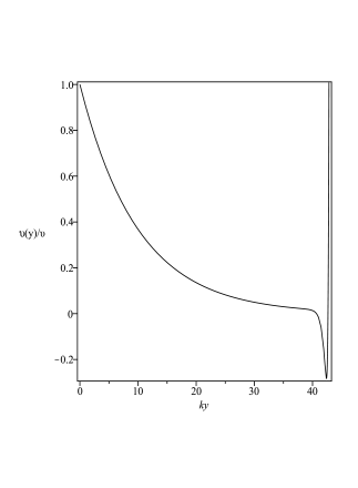
Figure 1: The VEV profile under $(D,D)$ BCs as a function of extra dimension for $\aleph=34$ in the absence of brane potential with $\Omega<0$ and a positive tension visible brane. We take $\upsilon\equiv\upsilon_{0,1,2,L}\equiv M^{\frac{3}{2}}_{pl}$, $k\equiv M_{pl}$, $\nu=2.1$, $M_{pl}=2.4\times 10^{18}GeV$ .

In figure $1$ the VEV profile for $\aleph=34$ is shown for the $AdS$ brane. In this figure we have assumed the brane tension of visible brane to be positive (see $eq.(66)$ for detail). we find that the pattern of localization is different from that of the $RS$ case. It is seen that the position of the IR brane shifts to the larger value of $z_{L}$ so the drastic change of the VEV profile occurs later than RS case. For this figure we have taken $\upsilon\equiv\upsilon_{0,1,2,L}\equiv M^{\frac{3}{2}}_{pl}$, $k\equiv M_{pl}$, $\nu=2.1$, $M_{pl}=2.4\times 10^{18}GeV$ .
For dS brane ,$\alpha\rightarrow-\alpha$ and $\beta\rightarrow-\beta$ therefore $A$ and $B$ can be written as

$$A=-\frac{\upsilon_{1}z_{L}^{(-\nu+2)}(1-\beta z_{L}^{2})-\upsilon_{2}(1-\beta)}{z_{L}^{(\nu+2)}(1-\alpha z_{L}^{2})(1-\beta)-z_{L}^{(-\nu+2)}(1-\beta z_{L}^{2})(1-\alpha)},$$ (24)

and

$$B=\frac{\upsilon_{1}z_{L}^{(\nu+2)}(1-\alpha z_{L}^{2})-\upsilon_{2}(1-\alpha)}{z_{L}^{(\nu+2)}(1-\alpha z_{L}^{2})(1-\beta)-z_{L}^{(-\nu+2)}(1-\beta z_{L}^{2})(1-\alpha)}.$$ (25)

By utilizing the above form of $A$ and $B$ in $eq.(13)$ the VEV profile of bulk scalar field is obtained for dS brane. We investigate this VEV profile for large and small values of $\omega$. We find that for the small values of positive brane cosmological constant the VEV profile has tiny difference with respect to the RS case.

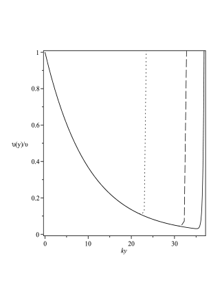
Figure 2: The dependence of VEV profile under $(D,D)$ BCs for large positive brane cosmological constant with $\aleph=20$ (dotted line), $\aleph=28$ (dashed line) and $\aleph=\infty$ (solid line i.e., RS case) . We take the same values for other parameter as ones in Figure $1$ .

In figure.$2$ we show the results for the large positive brane cosmological constant, namely $\aleph=20$ (dotted line) and $\aleph=28$ (dashed line). For the sake of comparison we also include $\aleph=\infty$ (solid line i.e., RS case). It is observed that the profile localizes near the IR brane. But the location of the IR brane is different in comparison to the RS case (see $eq.(69)$ of the appendix.
In $(D,N)$ case, the boundary conditions can be given by

$$\upsilon(1)=\upsilon_{1},\quad\quad\quad\partial_{z}\upsilon(z)|_{z=z_{L}}=0.$$ (26)

Then, for AdS brane they are written down by

$$A(1+\alpha)+B(1+\beta)=\upsilon_{1},$$ (27)

and

$$Az_{L}^{\nu+2}(v+2+\alpha(\nu+4)z_{L}^{2})-Bz_{L}^{-(\nu-2)}(\nu-2+\beta(\nu-4)z_{L}^{2})=0.$$ (28)

These lead to

$$A=\frac{\upsilon_{1}z_{L}^{(-\nu+2)}[(\nu-2)+\beta z_{L}^{2}(\nu-4)]}{z_{L}^{(-\nu+2)}(1+\alpha)[(\nu-2)+\beta z_{L}^{2}(\nu-4)]+z_{L}^{(\nu+2)}(1+\beta)[(\nu+2)+\alpha z_{L}^{2}(\nu+4)]},$$ (29)

and

$$B=\frac{\upsilon_{1}z_{L}^{(\nu+2)}[(\nu+2)+\alpha z_{L}^{2}(\nu+4)]}{z_{L}^{(-\nu+2)}(1+\alpha)[(\nu-2)+\beta z_{L}^{2}(\nu-4)]+z_{L}^{(\nu+2)}(1+\beta)[(\nu+2)+\alpha z_{L}^{2}(\nu+4)]}.$$ (30)

By substituting the above form of $A$ and $B$ in $eq.(9)$ the VEV profile in $(D,N)$ case of boundary conditions is obtained.

3.2 $(N,D)$ case

Next, we consider the $(N,D)$ case. These boundary conditions can be described by

$$\partial_{z}\upsilon(z)|_{z=1}=0,\quad\quad\quad\upsilon(z_{L})=\upsilon_{2}.$$ (31)

For negative brane cosmological constant, they are

$$A(\nu+2+\alpha(\nu+4))-B(\nu-2+\beta(\nu-4))=0,$$ (32)

and

$$Az_{L}^{\nu+2}(1+\alpha z_{L}^{2})+Bz_{L}^{(-\nu+2)}(1+\beta z_{L}^{2})=\upsilon_{2}.$$ (33)

These lead to

$$A=\frac{\upsilon_{2}[(\nu-2)+\beta(\nu-4)]}{z_{L}^{(-\nu+2)}(1+\beta z_{L}^{2})[(\nu+2)+\alpha(\nu+4)]+z_{L}^{(\nu+2)}(1+\alpha z_{L}^{2})[(\nu-2)+\beta(\nu-4)]},$$ (34)

and

$$B=\frac{\upsilon_{2}[(\nu+2)+\alpha(\nu+4)]}{z_{L}^{(-\nu+2)}(1+\beta z_{L}^{2})[(\nu+2)+\alpha(\nu+4)]+z_{L}^{(\nu+2)}(1+\alpha z_{L}^{2})[(\nu-2)+\beta(\nu-4)]}.$$ (35)

Like pervious subsection we substitute the above form of $A$ and $B$ in $eq.(9)$ to obtain the VEV profile in $(N,D)$ case of boundary conditions.

3.3 $(N,N)$ case

Finally, we investigate the $(N,N)$ case. These boundary conditions are

$$\partial_{z}\upsilon(z)|_{z=1}=0,\quad\quad\quad\partial_{z}\upsilon(z)|_{z=z_{L}}=0.$$ (36)

Then, for AdS brane they are written down by

$$A(\nu+2+\alpha(\nu+4))-B(\nu-2+\beta(\nu-4))=0,$$ (37)

and

$$Az_{L}^{\nu+2}(\nu+2+\alpha(\nu+4)z_{L}^{2})-Bz_{L}^{-(\nu-2)}(\nu-2+\beta(\nu-4)z_{L}^{2})=0.$$ (38)

We find that like RS model there is no solution to satisfy the above boundary conditions except for a trivial one, $(A,B)=(0,0)$ which is not of physical interest.
In this section we studied the VEV profile of a bulk scalar field under four boundary conditions on a generalized warped brane-world model in the absence of brane localized potential. We found that the VEV profiles depend on the vanishingly small brane cosmological constant.

4 VEV profiles in the presence of brane localized potentials

In this section, we formulate the VEV profiles of the bulk scalar field in a case with brane localized scalar potentials in the generalized Randall-Sundrum model. The action of a bulk field in the presence of brane potentials reads as

$$S=\int d^{4}x\int_{0}^{L}dye^{-4A(y)}[-e^{2A(y)}|\partial_{\mu}\Phi|^{2}-|\partial_{y}\Phi|^{2}-V-\delta(y)V_{0}-\delta(y-L)V_{L}].$$ (39)

The variation of the action is

$$\delta S=\int d^{4}x\int_{0}^{L}dye^{-4A(y)}[\delta\Phi_{X}(\rho\Phi_{X}-\frac{\partial V}{\partial\Phi_{X}})$$

$$+\delta(y)\delta\Phi_{X}(+\partial_{y}\Phi_{X}-\frac{\partial V_{0}}{\partial\Phi_{X}})+\delta(y-L)\delta\Phi_{X}(-\partial_{y}\Phi_{X}-\frac{\partial V_{L}}{\partial\Phi_{X}})].$$ (40)

From above equation the Dirichlet boundary condition is the same as $eq.(17)$ while the Neumann boundary condition should be modified as

$$\pm\partial_{y}\Phi_{X}-\frac{\partial V_{\eta}}{\partial\Phi_{X}}|_{y=\eta=0,L}=0.$$ (41)

In this paper we seek to generalize the Randall-Sundrum model and moreover we want to investigate the GW mechanism. Therefore we use the brane potentials as $[2,4,10]$

$$V_{\eta}=\lambda_{\eta}(|\Phi|^{2}-\frac{v_{\eta}^{2}}{2})^{2}=\frac{\lambda_{\eta}}{4}(\Phi_{R}^{2}+\Phi_{I}^{2}-v_{\eta}^{2})^{2},$$ (42)

where $\lambda_{0}$ and $\lambda_{L}$ stand for the brane tension and $\upsilon_{0}$ and $\upsilon_{L}$ are the VEV of the bulk scalar field on the UV and IR brane respectively. By utilizing the above scalar potentials we study the VEV profile in the case with brane localized potential in the generalized RS model. We notice that like the RS model, the $(D,D)$ boundary conditions in this case is the same as one for $(D,D)$ case with brane potentials.
For some other choices of the brane potentials see $[8]$.

4.1 $(D,N)$ case

Here, we consider the $(D,N)$ case that can be given by

$$\upsilon(1)=\upsilon_{1}\quad\quad\quad\partial_{z}\upsilon(z)|_{z=z_{L}}+\frac{\partial V_{L}}{\partial\Phi}|_{z=z_{L}}=0.$$ (43)

For AdS brane they are written down by

$$A(1+\alpha)+B(1+\beta)=\upsilon_{1},$$ (44)

and

$$k[Az_{L}^{\nu+2}(\nu+2+\alpha(\nu+4)z_{L}^{2})-Bz_{L}^{-(\nu-2)}(\nu-2+\beta(\nu-4)z_{L}^{2})]+$$

$$\lambda_{L}(Az_{L}^{\nu+2}(1+\alpha z_{L}^{2})+Bz_{L}^{(-\nu+2)}(1+\beta z_{L}^{2}))[(Az_{L}^{\nu+2}(1+\alpha z_{L}^{2})+Bz_{L}^{(-\nu+2)}(1+\beta z_{L}^{2}))^{2}-\upsilon_{L}^{2}]=0.$$ (45)

We should remember that when the coupling in the boundary potential is infinite, the Neumann boundary conditions turn to Dirichlet one if we choose $\upsilon_{L}=\upsilon_{2}$.
When the boundary quartic coupling is finite, the numerical calculation indicates that $A\ll B\simeq z_{L}^{\nu-2}\upsilon_{L}(1-\beta z_{L}^{2})$ as a solution of $eq.(44)$ and $eq.(45)$. For the small boundary quartic coupling, $A$ and $B$ can be approximated by

$$A\simeq\chi B[\frac{\nu-2+\beta z_{L}^{2}(\nu-4)}{\nu+2+\alpha z_{L}^{2}(\nu+4)}]z_{L}^{-2\nu}$$ (46)

and

$$B\simeq\sqrt{\upsilon_{L}^{2}+\frac{k(1-\chi)[\nu-2+\beta z_{L}^{2}(\nu-4)]}{\lambda_{L}(1+\beta z_{L}^{2})}}\frac{z_{L}^{\nu-2}}{1+\beta z_{L}^{2}},$$ (47)

where $\chi$ is determined by $eq.(44)$ and numerical calculation shows that $\chi\simeq O(1)$ and $\chi=1$ for $\lambda_{L}=0$. Also, $\chi$ is limited by

$$\chi\leq 1+\frac{\lambda_{L}(1+\beta z_{L}^{2})\upsilon_{L}^{2}}{k[\nu-2+\beta z_{L}^{2}(\nu-4)]}.$$ (48)

Figure 3: The VEV profile for negative induced brane cosmological constant with positive brane tension for $\aleph=33$ (dotted line), $\aleph=34$ (dashed line) and $\aleph=\infty$ (solid line i.e., RS case) in the $(D,N)$ case for $\widetilde{\lambda}_{L}=100$. The values of other parameters of the model are the same as the ones in Figure $1$ .

In Fig. $3$ we show the dependence of VEV profile for negative induced brane cosmological constant with positive brane tension with $\widetilde{\lambda}_{L}=100$.

4.2 $(N,D)$ case

For the $(N,D)$ case, these boundary conditions given by

$$\partial_{z}\upsilon(z)|_{z=1}-\frac{\partial V_{0}}{\partial\Phi}|_{z=1}=0,\quad\quad\quad\partial_{z}\upsilon(z)|_{z=z_{L}}=0.$$ (49)

Then, for negative brane cosmological constant they are written down by

$$k[A(\nu+2+\alpha(\nu+4))-B(\nu-2+\beta(\nu-4))]$$

$$-\lambda_{0}(A(1+\alpha)+B(1+\beta))[(A(1+\alpha)+B(1+\beta))^{2}-\upsilon_{0}^{2}]=0,$$ (50)

and

$$Az_{L}^{\nu+2}(1+\alpha z_{L}^{2})+Bz_{L}^{(-\nu+2)}(1+\beta z_{L}^{2})=\upsilon_{2}.$$ (51)

Numerical calculation indicates that $A\sim B\sim\frac{\upsilon_{2}}{z_{L}^{2}(1+\alpha z_{L}^{2})}$ and for small $\lambda_{0}$, $\widetilde{\lambda}_{0}\leq O(0.01)$, $A$ and $B$ are approximated by

$$A\simeq(1-\frac{\Gamma_{1}}{\Gamma_{1}+\Gamma_{2}z_{L}^{2\nu}})\frac{\upsilon_{2}z_{L}^{-(\nu+2)}}{1+\alpha z_{L}^{2}},$$ (52)

and

$$B\simeq(\frac{\Gamma_{1}}{\Gamma_{1}+\Gamma_{2}z_{L}^{2\nu}})\frac{\upsilon_{2}z_{L}^{\nu-2}}{1+\beta z_{L}^{2}}.$$ (53)

Where

$$\Gamma_{1}=(1+\beta z_{L}^{2})[k(\nu+2+\alpha(\nu+4))+\lambda_{0}\upsilon_{0}^{2}(1+\alpha)],$$ (54)

and

$$\Gamma_{2}=(1+\alpha z_{L}^{2})[k(\nu-2+\beta(\nu-4))-\lambda_{0}\upsilon_{0}^{2}(1+\beta)].$$ (55)

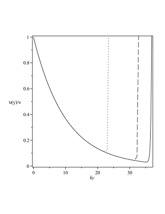
Figure 4: The VEV profile for large positive brane cosmological constant with $\aleph=20$ (dotted line), $\aleph=28$ (dashed line) and $\aleph=\infty$ (solid line i.e., RS case)in the $(N,D)$ case for $\widetilde{\lambda}_{0}=100$. The values of other parameters of the model are the same as the ones in Figure $1$ .

Figure $4$ shows the VEV profile for large positive brane cosmological constant, when $\widetilde{\lambda}_{0}=100$.

4.3 $(N,N)$ case

The $(N,N)$ case of boundary conditions for AdS brane are

$$\partial_{z}\upsilon(z)|_{z=1}-\frac{\partial V_{0}}{\partial\Phi}|_{z=1}=0,\quad\quad\quad\partial_{z}\upsilon(z)|_{z=L}+\frac{\partial V_{L}}{\partial\Phi}|_{z=L}=0.$$ (56)

Then, the boundary conditions can be written down as

$$k[A(\nu+2+\alpha(\nu+4))-B(\nu-2+\beta(\nu-4)]$$

$$-\lambda_{0}(A(1+\alpha)+B(1+\beta))[(A(1+\alpha)+B(1+\beta))^{2}-\upsilon_{0}^{2}]=0,$$ (57)

and

$$k[Az_{L}^{\nu+2}(\nu+2+\alpha(\nu+4)z_{L}^{2})-Bz_{L}^{-(\nu-2)}(\nu-2+\beta(\nu-4)z_{L}^{2})]+$$

$$\lambda_{L}(Az_{L}^{\nu+2}(1+\alpha z_{L}^{2})+Bz_{L}^{(-\nu+2)}(1+\beta z_{L}^{2}))[(Az_{L}^{\nu+2}(1+\alpha z_{L}^{2})+Bz_{L}^{(-\nu+2)}(1+\beta z_{L}^{2}))^{2}-\upsilon_{L}^{2}]=0.$$ (58)

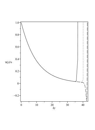
Figure 5: The VEV profile for negative induced brane cosmological constant with positive brane tension for $\aleph=33$ (dotted line), $\aleph=34$ (dashed line) and $\aleph=\infty$ (solid line i.e., RS case) in the $(N,N)$ case for $\widetilde{\lambda}_{0}=100,\widetilde{\lambda}_{L}=100$. The values of other parameters of the model are the same as the ones in Figure $1$ .

In the limit of very small boundary couplings, $\widetilde{\lambda}_{0}\ll O(0.01)$ and $\widetilde{\lambda}_{L}\ll O(0.1)$, $A$ and $B$ are zero but for large boundary quartic couplings which is considered in GW mechanism we have

$$A_{GW}\simeq-\upsilon_{0}\frac{(1+\beta z_{L}^{2})}{\Delta_{1}}z_{L}^{-2\nu}+\upsilon_{L}\frac{(1+\beta)}{\Delta_{1}}z_{L}^{-(\nu+2)},$$ (59)

and

$$B_{GW}\simeq\upsilon_{0}\frac{(1+\alpha z_{L}^{2})}{\Delta_{1}}(1+\frac{\Delta_{2}}{\Delta_{1}}z_{L}^{-2\nu})-\upsilon_{L}\frac{(1+\alpha)}{\Delta_{1}}z_{L}^{-(\nu+2)}.$$ (60)

Where

$$\Delta_{1}=(1+\beta)(1+\alpha z_{L}^{2}),$$ (61)

and

$$\Delta_{2}=(1+\alpha)(1+\beta z_{L}^{2}).$$ (62)

Here we numerically analyze the VEV profile for finite boundary couplings. The result is shown in Figure $5$ for large values of $\widetilde{\lambda}_{0}$ and $\widetilde{\lambda}_{L}$. At the end of this section we reconsider the realizations of the GW mechanism under general boundary conditions in the generalized RS model. In the GW mechanism the effective potential for the modulus can be generated by the total action integral of a bulk scalar field with quartic interactions localized in two $3-$branes. The bulk scalar field acts an important role to stabilize the radion which yields a compactification scale in terms of VEVs profile of the scalar field at two branes. The VEV of the bulk scalar can be obtained by solving the equation of motion.
Recently, this mechanism was studied in the generalized warped brane models with a nonzero brane cosmological constant by $[9]$. They have been obtained the modulus stabilization condition both for positive and negative values of the brane cosmological constant which increases (decreases) from RS value with increasing $\omega^{2}$.
we have investigated the unknown coefficients A and B of the VEV profile of the bulk scalar field in the generalized RS model by imposing boundary conditions which are given in the sections $3$ and $4$. It is well known that the $(N,N)$ type boundary conditions given by $eq.(59)$ and $(60)$ should be taken in the GW mechanism. The situation in the generalized warped model is similar to RS warped model as discussed in Ref. $[10]$. When the boundary quartic couplings $\lambda_{0}$ and $\lambda_{L}$ are large the $(N,N)$ BCs which imposed in the GW mechanism are equivalent to $(D,D)$ ones given in $(20)$ if we take $\upsilon_{1}=\upsilon_{0}$ and $\upsilon_{2}=\upsilon_{L}$, so by this assumption in the limit of large boundary couplings, A and B given by $eq.(21)$ and $eq.(22)$ are $A\simeq A_{GW}$ and $B\simeq B_{GW}$, therefore the GW mechanism can be realized in the $(D,D)$ case with appropriate VEV profile.
In the generalized warped model as mentioned in Ref. $[10]$, when the brane localized potential is considered, GW mechanism can also work in $(N,D)$ and $(D,N)$ BCs with large boundary quartic couplings. The GW mechanism can not work when one of the boundary coupling $\lambda_{0}$ or $\lambda_{L}$ becomes small in $(N,N)$ case.

5 Conclusions

In the RS model a negative tension visible brane is utilized to describe our Universe. However, Such negative tension branes are unstable. Hence in this work we considered a generalized RS warped model.
In this paper we investigated a bulk scalar field under Dirichlet and Neumann boundary conditions in a generalized RS warped model with a non zero cosmological constant on the brane. First we have obtained the profiles of VEV of the bulk scalar in the absence of brane localized potential for the negative and positive brane cosmological constant. We find that:
$(1)$ For an AdS visible brane with negative brane tension the results are similar to RS case.
$(2)$ However for an AdS visible brane with positive brane tension the results are different from the RS case. In this case the VEV profile undergo sudden changes near the IR brane. Moreover we see that the IR brane is displaced from it’s RS location. The coefficients $A$ and $B$ are functions of the length of the stabilized modulus. Hence the change of the length of the stabilized modulus modifies the shape of the VEV in comparison to the RS case.
$(3)$ For a dS visible brane the results for small values of $\omega^{2}$ are not different from the RS case. But for larger values of $\omega^{2}$ we have departures from the RS result.
Next we have considered the VEV profiles under general boundary conditions in the presence of brane localized potential for non zero brane cosmological constant. We find that to see drastic changes of the profile near the IR brane for an AdS visible brane with positive brane tension the value of $\widetilde{\lambda}_{L}\sim O(1)$ in the RS case but the value of $\widetilde{\lambda}_{L}\sim O(10)$ in the present case.
We have also verified GW mechanism in the generalized RS model with Dirichlet and Neumann Boundary conditions. Analogous to RS model $[10]$ the GW mechanism can work under non zero Dirichlet BCs with appropriate VEVs in the generalized RS model. It will be interesting to use these results to study the Dirichlet Higgs as radion stabilizer in the generalized warped campactification.
Our analysis of consistent boundary conditions is similar to that of Csaki, et. al. $[17]$. It is possible to extend this work by studying the behavior of the bulk scalar field on the warped five dimension by utilizing the background field method, separating the field into classical and quantum fluctuation parts and to investigate the phenomenological consequences of the profile of the scalar field $[10]$.
There are quantum corrections, from Casimir effect and induced gravity on the brane. One requires that the brane world metric be a solution of the quantum-corrected Einstein equations. For the RS model this issue has been addressed in Refs. $[18,19]$. From $eq.(12)$ we see that in the generalized RS model $A(y)=k|y|$ plus extra small term due to the curved branes. In the RS model the sum of brane tensions of two branes are zero. However in the generalized RS model this sum is not zero $[3]$. Hence the discussion of the issue of self-consistency is different from that of the RS model. However it is reasonable to expect that GRS be self consistent for some specific values of the parameters of the model .
The analysis presented in this work we have ignored the backreaction of the scalar field on the spacetime geometry. The stress tensor for the scalar field in the limit of large modulus can be obtained $[4]$ . For the $(N,N)$ case with large boundary coupling,stress tensor for the scalar field can we find that if $v^{2}_{0}\Delta^{2}_{1}/M_{5}^{3}<<1$, $v^{2}_{L}\Delta^{2}_{1}/M_{5}^{3}<<1$ and $m^{2}/k^{2}<<1$, then one can neglect the stress tensor for the scalar field in comparison to the stress tensor induced by the bulk cosmological constant. Furtheremore the parameters of the bulk and brane potential are constrained by these inequalities.
In this work our choices for the bulk and the brane potentials were those of Ref. $[2]$. Other choices for the bulk potential and brane potentials are possible. The potential for the $GW$ scalar $\Phi$ in the bulk $[20]$ has the general form of $V(\Phi)=m^{2}\Phi^{2}+C_{3}\Phi^{3}+C_{4}\Phi^{4}+......$ . It would be interesting to study the VEV profiles of the bulk scalar field in such generalized warped models.
In a previous work we studied the case of a scalar field non-minimally coupled to the Ricci curvature scalar $[21]$. The case of massless, conformally coupled scalar field are self-conistent after the inclusion of quantum corrections. Hence it will be of interest to consider massless, conformally coupled scalar field in the generalized RS framework.

Appendix : The variation of $kr\pi$ and the brane tensions

In the $RS$ $[2]$ case the brane tension of the visible brane is negative and to solve the hierarchy problem the value of $kr\pi=36.84$.
The situation is different in the generalized $Randall-Sundrum$ model.
This subject is discussed in Ref. $[3]$. Here we provide a concise presentation.

The AdS case

If we denote $\varsigma=kr\pi$ then for the case where the cosmological constant of the brane is negative we have $[3]$

$$e^{-\varsigma}=\frac{10^{-n}}{c_{1}}[1\pm\sqrt{1+\omega^{2}10^{2n}}],$$ (63)

with $c_{1}=1+\sqrt{1-\omega^{2}}$. Let $\varsigma_{1}$ and $\varsigma_{2}$ corresponds to the plus and minus sign respectively. The $\varsigma_{1}$ case is not much different from the $RS$ case. But the $\varsigma_{2}$ is quite distinct from the $RS$ case. In the limit $\aleph-2n\gg 1$

$$\varsigma_{1}\simeq nln10+\frac{1}{4}10^{-(\aleph-2n)}\qquad\varsigma_{2}\simeq(\aleph-n)ln10+ln4,$$ (64)

the value of $\varsigma_{2}$ can be as large as $250$.
Next we will show below in this situation the brane tension of the visible brane is positive. As far as the stability of the brane is concern this is a desirable feature. To compute the brane tension $U_{vis}$ of the AdS case we rewrite the brane tension of the visible brane of Ref. $[3]$ as

$$U_{vis}=12M^{3}k[\frac{1-(c_{1}e^{-\xi}\omega^{-1})^{2}}{1+(c_{1}e^{-\xi}\omega^{-1})^{2}}].$$ (65)

Now inserting $eq.(63)$ in $eq.(65)$ and with $\omega^{2}=10^{-\aleph}$, the correct form of brane tension of the visible brane is

$$U_{vis}=(12M^{3}k)\frac{1-10^{\aleph-2n}(1\pm\sqrt{1-10^{-(\aleph-2n)}})^{2}}{1+10^{\aleph-2n}(1\pm\sqrt{1-10^{-(\aleph-2n)}})^{2}}.$$ (66)

And finally from this result we can compute the brane tension in the limit where $\aleph-2n\gg 1$. For the plus sign case the brane tension for the visible brane is negative and it is given

$$U_{vis-1}\simeq-12M^{3}k.$$ (67)

Which is in agreement with the result of Ref. $[3]$.
But for the minus sign case the brane tension for the visible brane is positive and it is given

$$U_{vis-2}\simeq 12M^{3}k.$$ (68)

Which differs from the result of Ref. $[3]$ by a factor $3$.

The dS case

When the cosmological constant of the brane is positive we have

$$e^{-\varsigma}=\frac{10^{-n}}{c_{2}}[1+\sqrt{1+\omega^{2}10^{2n}}],$$ (69)

with $c_{2}=1+\sqrt{1+\omega^{2}}$. It turns out that the brane tension of the visible brane is negative for the entire range of the positive values of $\Omega$. However the difference with the $RS$ case is due to the value of $\varsigma$. For instance for $\aleph=20$ we obtain $\varsigma=23.7$.

References

- [1] N. Arkani-Hamed, S. Dimopoulos and G. Dvali, Phys. Lett. B 429 (1998) 263.
- [2] L. Randall and R. Sundrum, Phys. Rev. Lett. 83 (1999) 3370.
- [3] S. Das, D. Maity and S. SenGupta, JHEP 0805 (2008) 042.
- [4] W. D. Goldberger and M. B. Wise, Phys. Rev. Lett. 83 (1999) 4922.
- [5] O. DeWolfe, D. Z. Freedman, S. S. Gubser and A. Karch, Phys. Rev. D 62 (2000) 046008.
- [6] A. Dey, D. Maity and S. SenGupta, Phys. Rev. D 75 (2007) 107901.
- [7] W. D. Goldberger and M. B. Wise, Phys. Lett. B 475 (2000) 275.
- [8] J. M. Cline, H. Firouzjahi, Phys.Rev. D 64 (2001) 023505.
- [9] R. Koley, J. Mitra and S. SenGupta, Euro. Phys. Lett. 85 (2009) 41001.
- [10] N. Haba, K. Oda and R. Takahashi, JHEP 1105 (2011) 125.
- [11] H. Davoudiasl, S. Gopalakrishna, E. Ponton, and J. Santiago, New J. Phys. 12 (2010) 075011.
- [12] C. Csaki, arXiv:hep-ph/0404096 [hep-ph].
- [13] R. Sundrum, arXiv:hep-th/0508134 [hep-th].
- [14] J. M. Cline, J. Descheneau, M. Giovannini and J. Vinet, JHEP 06 (2003) 048.
- [15] C. Csaki, J. Erlich, C. Grojean and T. J. Hollowood, Nucl. Phys. B 584 (2000) 359.
- [16] H. P. Nilles, A. Papazoglou and G. Tasinato, Nucl. Phys. B 677 (2004) 405.
- [17] C. Csaki, C. Grojean, H. Murayama, L. Pilo and J. Terning, Phys. Rev. D 69, 055006 (2004) 05500.
- [18] A. Flachi and D. J. Toms, Nucl. Phys. B 610 (2001) 144.
- [19] A. Knapman and D. J. Toms, Phys. Rev. D 69 (2004) 044023.
- [20] Z. Chacko, A. Rashmish, K. Mishra, and D. Stolarskia, JHEP 1309 (2013) 121.
- [21] A. Tofighi, M. Moazzen, Mod. Phys. Lett. A 28 (2013) 1350044.