Machine Learning for Machine Data from a CATI Network

Abstract

This is a machine learning application paper involving big data. We present high-accuracy prediction methods of rare events in semi-structured machine log files, which are produced at high velocity and high volume by NORC’s computer-assisted telephone interviewing (CATI) network for conducting surveys. We judiciously apply natural language processing (NLP) techniques and data-mining strategies to train effective learning and prediction models for classifying uncommon error messages in the log—without access to source code, updated documentation or dictionaries. In particular, our simple but effective approach of features preallocation for learning from imbalanced data coupled with naive Bayes classifiers can be conceivably generalized to supervised or semi-supervised learning and prediction methods for other critical events such as cyberattack detection.

We dedicate this article to Fritz Scheuren, ASA Fellow and former ASA President,
on the occasion of his 75th birthday.

1 Introduction

The data we processed and analyzed in this study stemmed from NORC’s computer-assisted telephone interviewing (CATI) system. The CATI network can automatically retrieve and dial a household phone number from a random sample, drawn from a comprehensive vendor-prepared phone list, so NORC can conduct surveys and collect data on topics of public interest, and compute statistics representative of the relevant population. Survey data, traditionally, consist of relatively small samples and are often analyzed by statistical techniques (Wolter 2007). More recently, as sizes, varieties, and complexities of survey data grow faster than ever, novel machine learning methods especially those applicable to text data are sought after for knowledge discovery and predictive analysis at a large scale (see Murphy et al. 2014, for instance), an example being topic models (Blei et al. 2003) applied to cluster survey responses by Wang and Mulrow (2014). Our work here using naive Bayes method to classify machine messages is another attempt in such a direction.

The NORC CATI system is a vendor-developed black box; we do not have access to the codebase. It is a distributed system and the infrastructure environment is complex, mostly maintained by NORC’s information technology department on a daily basis. The system has a front-end interface running on a web browser with whom an interviewer interacts to initiate, conduct, and complete a phone survey. There are backend servers that persist important and sometimes personally identifiable data into databases and machine messages into rolling log files. At any moment during a business hour, there is data traffic over our secure network going back and forth among front-end and backend components. These data are typically text, numeric, voice and image files to and from interactive dynamic webpages called HTTP frames. The smallest components of network data are known as packets. For the purpose of performance profiling, we collect information from HTTP frames down to the level of packets, as well as machine log files and SQL database trace tables. NORC has two large call centers across the U.S. continent: one is located in Chicago, Illinois and the other one in Las Vegas, California. At full capacity, there are as many as 500 interviewers working with multiple application servers and SQL databases in Chicago. Figure 1 is a simplified pictorial representation of NORC’s distributed CATI network.

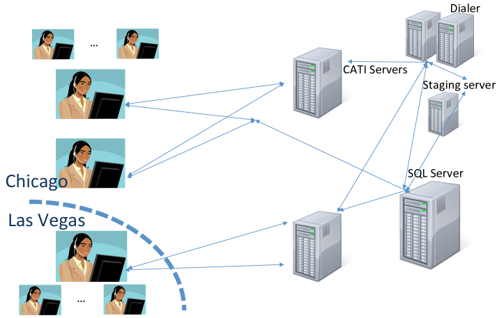
Figure 1: A pictorial representation of NORC’s distributed CATI network.

On June 4, 2014, during a regular business hour, our network and database engineers collected web transactions and packet information on three client machines in our network. For the three clients, two were in Chicago and one was in Las Vegas; the configuration was made to gauge the effects of latency, i.e., the delay in time incurred in transferring data over a long distance.

The HTTP frames and packet data were compressed (saz, pcap) files. We also collected server log files and database trace tables. For ease of analysis, we decompressed all files and if necessary transformed them into text format. As a result, during that test-data collection hour, we amassed almost 30 gigabytes (GB) of data. It is a potential source of big data coming to NORC at high velocity and high volume. Here is a quick summary of our collected machine data:

1. Raw data (compressed): 1.8 GB; 267 files.

   1. HTTP frames: 86.9 MB (megabytes)

   2. Packets data: 1.7 GB

   3. Server log: 31.5 MB

   4. Database trace table: 685 MB

2. Decompressed data (text): 28.9 GB; 27,785 files.

3. Analysis results (text) : 15.7 MB; 15 files.

We applied various methods for analyzing the datasets for causes of bottleneck performance in the system that sometimes occur during a phone connection process. In addition, from machine-generated time stamps, we measured the time lapses between comparable web transactions and log messages; and we learnt about the significant effects of latency (Choi et al. 2014) though we will not go into further details. In the rest of this report, we focus on natural language processing (NLP) and machine-learning methods we applied on the collected data.

Here is an outline of this report: In Section 2, we detail some of the characteristics and challenges of server log data. In Section 3, we develop data preprocessing methods, model building process, and performance evaluation criteria. Concrete examples are included for illustration in Section 4. Lastly, we conclude with a few comments and thoughts of future work in Section 5.

2 Data from Server Log 

In the absence of dictionary and metadata, we set out to learn about the characteristics of the CATI machine language. In particular, we focused on messages in the collected server log files, one of the four key components of the raw data (see Section 1). Over the server side, such communication is of high frequency and is captured in text files. The messages are usually intended for network administrators and application programmers for performance tuning or problem shooting. These log messages are lines after lines of records about the internal states of the servers during run-time (e.g., key variable values, memory usage) and traces of interactions and communication of the server with other network components. At times when a server experiences stress due to, say, resource shortage, or not behaving as programmed, it will issue warnings or error messages. These log events are typically semi-structured, starting with a time stamp, followed by some text of heterogeneous data, which consist of message type that may take on values such as FINE, DEBUG, INFO, WARNING, ERROR, or FATAL. Sometimes after the message type, we see a few additional optional fields such as program filename, method name, class name, and line number at which the message is defined. Lastly we have the technical content of the message event. Hence applying NLP techniques and machine learning methods for analysis seems fitting.

Example 2.1

In the following log message, 20140604 103903.913 is the time stamp of the format YYYYMMDD HHMMSS.ttt, where YYYY represents year in four digits; MM and DD for month and day, respectively; HHMMSS for hour, minutes, and seconds; ttt for milliseconds. Error is the message type, which is followed by the message content indicating the occurrence of an undesirable timeout event (not receiving any or an expected response from a user or a network component within a time window):

20140604 103903.913 Error: ProntoEventServer. PE_Client removed on
Duration 8453ms Timeout 502ms StackSize 90

In our CATI system, message fields are, however, not always standardized, rendering some messages appearing irregular and harder to read than usual by human experts or computer programs. We give a few examples immediately below for illustration of such difficulties.

Example 2.2

Each of the message field sometimes has missing or extra components. In this example, the time stamp has no year information and there is an extra slash between the month and the day, followed by a five-digit sequence ($02488$ below), which is unclear to us what it means.

06/04 142452.865|02488|error | CAlarmFilter |general |onXmlRead>
xml element "alarms" is ignored

Example 2.3

In this example, the optional fields appear after—instead of before—the message content. Their order and formats could appear quite different in other messages.

20140604 063402.441 ERROR : dcb_open(dcbB1D1,NULL)=success (#=0)
InstanceName=TDialogicDevice dcbB1D1
ClassName=TDialogicConferenceDevice MethodName=Initialize
FileName=.\DialogicDeviceConference.cpp LineNumber=138

Among all message types, errors are of particular importance to system administrators or software engineers. They are the distress signals whereas messages of other types may be considered “white noise.” Nonetheless, it is not always a straightforward matter to tell whether a message is an error in our CATI log files. Example 2.4 below lists some of the abnormal cases we encountered.

Example 2.4

Message type in the following log event is CriticalError, which may, or may not, indicate a more serious kind of error:

20140604 120353.022 CriticalError: Report: SQL Exception: Query:
sp_Pronto_AddAgentActivity

In other cases, an error message may have no mention of the word “error” anywhere, or the value of message type is missing. The following are two such examples, where the first one seems to be an error whereas the second one is not:

20140604 144846.946 04776 A:006 line 5 still in dialing mode.
Sending error 27 to dial command before ending the session

20140604 064238.541 11DE6B80: LineCallSpecificLine(1) return
ADVR_NO_ERROR

The next example is a message that concludes with “no error.” Hence the appearance of the word “error” in message content may not necessarily represent an erroneous event:

06/04 145011.634|01384 | debug |dispatcher |L:000 |LogMetaEventInfo>
E=GCEV_ANSWERED (802h) : gc_ResultInfo()=0h; gcVal=500h, Normal
completion ccId=6h, GC_DM3CC_LIB ccVal=0h, No Error

3 NLP and Naive Bayes Classifier 

The discussion so far has led to the question, among others, that in the presence of aforementioned or other abnormalities, how a log event could be accurately classified as an error or a non-error. One approach is to learn about the machine log features associated with known errors and characteristics of recognized non-errors, and then build a model to perform a binary classification of a message of unknown type as an error or not. We note that the notion of “error” here can be generalized to any event of interested outcome that can be annotated by human experts or inferred by computer programs. The problem of error classification is not necessarily too difficult, but it comes with some challenges for our CATI system, to name a few:

1. Software code is not available for tracing or modification.

2. Lack of (updated) documentation.

3. The machine language, that is programmers’ language, in log files is often incomprehensible. The log messages often contain many unreadable, unnatural variable names and values. No dictionary or sufficient metadata are available to us for lookup.

4. The event of interest, ERROR, occurs rarely ($<1\%$ of all events) because we do have a well-maintained and highly functional production system.

Previous works on extensive log analysis include Xu (2010) and Xu et al. (2010), which apply principal component analysis (PCA) for anomaly detection and decision trees for visualization. However, our problem appears to be more onerous due to lack of access to source code.

Our analysis consists of seven basic programmatic steps. The first three steps belong to the domain natural language processing. The last four steps are related to machine learning; we repeat them and adjust the input parameters ($p$, $n$, and $m$ below) if necessary, until the model performance in Step 7 is satisfactory.

1. Read every event line of a log file into three fields: time stamp, message type, and message content. If optional fields such as filename or method name are available, we consider them parts of the message content. To enhance the effectiveness of our reading task, we employ regular expressions in Python.

2. Assign a class to every event by looking at value of message type, i.e., set an outcome variable isError to true if message type contains the word “error” (case insensitive), and false otherwise.

3. Reduce all messages into tokens of words.

4. Select top $p$ most frequently seen words as features.

5. Learn on a time-consecutive training set of messages whose size, $n$, is user chosen.

6. Classify a test set of $m$ messages that happened after the training set messages.

7. Evaluate performance of the prediction model.

Our machine-learning method of choice in this study is naive Bayes classification—it could have been decision tree, random forest, or other models; see, for example, Han et al. (2012) for an overview of these methods. Here we give a succinct summary of the naive Bayes classifier. Given a training dataset $\{{a_{i}}\}_{i=1}^{n}$ and each item $a_{i}$’s class label $c_{i}\in\{C_{j}\}_{j=0}^{K}$. Suppose each $a_{i}$ has $p$ given feature values $\{X_{k}=x_{i,k}\}_{k=1}^{p}$. When a new data point $a_{n+1}$ with its property values $\{X_{k}=x_{n+1,k}\}_{k=1}^{p}$ come in, we want to classify it by estimating the probabilities of it belonging to each class $C_{j}$ given its features. In particular, when $K=1$, we have a binary classification problem. We use the shorthand $P(C_{j}|X)\equiv P(c_{n+1}=C_{j}|X_{k}=x_{n+1,k}\mbox{ for }k=1,\ldots,p)$. Then, by the Bayes theorem and assuming class conditional independence, we have

$$P(C_{j}|X)=\frac{P(X|C_{j})P(C_{j})}{P(X)} \quad\propto\quad\Pi_{k=1}^{p}P(X_{k}|C_{j})P(C_{j}),$$ (1)

product of the probabilities of the item’s features given a class and the proportion of the class, both estimated from the training set. The algorithm simply classifies the new data point to be in class $C_{J}$ such that $J=\arg\max_{j=0,\dots,K}P(C_{j}|X)$. Note that the quantity $P(X)$ in (1) can be omitted in the optimization process as it is the same across all classes.

The naive Bayes classifier is in practice a very efficient and robust algorithm even when the assumption of conditional independence may not hold for an input dataset; see, for example, López et al. (2013). When at a future time we know for certain about the class true value, $C_{J^{*}}$, of the data point $a_{n+1}$, we can then compare $C_{J^{*}}$ with the model’s previously predicted value $C_{J}$, and update the confusion matrix ${\left[\begin{smallmatrix}a&b\\ c&d\end{smallmatrix}\right]}$, where $a$ and $d$ are respectively the true positive and true negative counts, whereas $b$ and $c$ are the false positive and false negative counts. Note that $a+b+c+d=m$, the size of test set. We can then proceed to compute the prediction model’s accuracy and precision, which are defined as $\tfrac{a+d}{m}$ and $\tfrac{a}{a+b}$, respectively, as they are among the most common performance measures for a prediction model; see, for example, Han et al. (2012).

We use an open-source Python package called Natural Language Toolkit, or NLTK in short; see Bird et al. (2009). We started with a simple adaptation of the NLTK examples. Unfortunately it resulted in poor accuracy, memory exhaustion, and slow performance. There are a few strategies in implementation that we have found useful in overcoming the performance problems and generally resulting in better model predictiveness.

1. Exclude stop words (e.g., prepositions such as “of” and “from”) from the features because such frequently seen words are not predictive of errors or non-errors.

2. Change all words to lowercase in tokenization and feature selection processes. This reduces number of features without sacrificing predictive power of the model.

3. Exclude numbers from features. This strategy is found to be helpful in our study but may not always be effective in other cases.

4. Preallocate a significant number of features for learning from error messages. We cannot emphasize enough that this is the most important and effective strategy of all in our experience. Since error events are rare, features were quickly filled up by non-error content, and consequently the model would not have accumulated enough information about error events, resulting in poor predictive accuracy due to too small values of $P(X_{k}|C_{j})$ and $P(C_{j})$ in (1).

A common technique that we have not used is simulation or over-sampling of rare events during the training stage so as to increase the values of $P(X_{k}|C_{j})$ and $P(C_{j})$. For a comprehensive discussion of challenges and strategies for learning rare events, we refer readers to a recent review by López et al. (2013).

4 Examples 

In this section, we present two examples. Built on NLTK (version 3.0.0), we developed an object-oriented class in Python (version 2.7.10) called norc_class with simple interfaces for reading a text log file; tokenizing messages with NLTK’s function word_tokenize(); assigning labels; picking features; building models mainly based on methods train() and classify_many() in the NLTK class NaiveBayesClassifier; and last but not least, displaying results.

Example 4.1

We built a learning and prediction model with $p=562$ features selected from a training set of size $n=20,000$. The following results show that, on a test set of size $m=50,210$, with less than one percent errors, the trained classifier predicted only one error message incorrectly as non-error, given a total of $110$ error events; that is to say, the prediction model’s accuracy was $0.95$ and its precision was $0.99$. The two most predictive words of errors were “circuit” and “pronto”. The absence of the words “failure” and “dialogic”, or the presence of “*dlggctelapi” were most predictive of a non-error event (we use an asterisk to mask the vendor name).

len(documents) = 71210
len(features) = 562
len(train_set) = 20000
len(test_set) = 51210
n_errs = 697, percentage = 0.98

Confusion matrix =
[  109     1]
[ 2340 48760]
Accuracy [0-1] = 0.95. Precision [0-1] = 0.99
Most Informative Features
                 circuit = True          True : False  =  12799.6 : 1.0
                  pronto = True          True : False  =    163.4 : 1.0
                  failed = False        False : True   =    128.8 : 1.0
                dialogic = False        False : True   =    122.4 : 1.0
            *dlggctelapi = True         False : True   =     95.3 : 1.0

Example 4.2

In this example, the number of sample messages in the dataset was $97,832$ and about merely one percent were error messages. The first $n=88,049$ messages were used to build a naive Bayes classifier with $p=2,000$ features. On the test set consisting of the remaining $9,783$ messages, the model predicted error events at an accuracy of $0.97$ and a precision of $0.98$. The most predictive words of error messages were “exception”, “page”, “intweb”,“putting”, and “list”.

len(documents) = 97832
len(features) = 2000
len(train_set) = 88049
len(test_set) = 9783
n_errs = 1117, percentage = 1.14

Confusion matrix =
[ 100    2]
[ 243 9438]
Accuracy [0-1] = 0.97. Precision [0-1] = 0.98
Most Informative Features
               exception = True           True : False  =   4311.8 : 1.0
                    page = True           True : False  =   3569.3 : 1.0
                  intweb = True           True : False  =   2141.6 : 1.0
                 putting = True           True : False  =   1189.8 : 1.0
                    list = True           True : False  =    973.5 : 1.0

5 Conclusions 

We developed systematic ways of collecting and parsing data in NORC’s distributed CATI production network. By examples of event messages in server log files, despite their highly technical nature, we built performant supervised models for classification of rare error. The key enabling data preprocessing technique here is preallocation of features in memory dedicated to learning most frequently seen words of rare event messages.

For future work, we shall continue to refine and automate the naive Bayes classification model, making it incremental and with less memory and computational requirements. We could employ more robust techniques such as $k$-fold cross validation and ROC curves for model quality evaluation (Han et al. 2012). When the work is mature, we could port our prototype to Hadoop or Spark servers for large-scale (near) real-time analysis. We may also adapt our model to predict other events of business interests such as long wait time before a call is connected or delays in inbound calls. Lastly, it would be valuable to predict occurrence of a positive event in advance. Our preliminary models that learnt about each example as a brief time window of messages unfortunately yielded low accuracy (around the value of 0.6). The approach was not effective probably because many attributes from events leading up to errors became intermixed with those associated with non-errors—better models have yet to be developed.

References

- [1]
- [2] Bird, S., Klein, E., and Loper, E. (2009), Natural Language Processing with Python, O’Reilly Media, Inc.
- [3]
- [4] Blei, D. M., Ng, A. Y., and Jordan, M. I. (2003), “Latent Dirichlet Allocation,” Journal of Machine Learning Research, 3, 993–1022
- [5]
- [6] Choi, S.-C. T., Seeger, J., and Ware, S. (2014), “CATI Network Performance through Packet and Log Analysis,” [PowerPoint slides], NORC at the University of Chicago.
- [7]
- [8] Han, J., Kamber, M., and Jian P. (2012), Data Mining: Concepts and Techniques (3rd edition), Elsevier.
- [9]
- [10] López, V., Fernández, A., García, S., Palade, V., and Herrera, F. (2013), “An Insight into Classification with Imbalanced Data: Empirical Results and Current Trends on Using Data Intrinsic Characteristics,” Information Sciences 250, 113–141.
- [11]
- [12] Murphy, J., Hill, C. A., and Dean, E. (2014), Social Media, Sociality, and Survey Research, John Wiley & Sons, Inc.
- [13]
- [14] Wang, F. and Mulrow, E. (2014), “Analyzing Open-Ended Survey Questions Using Unsupervised Learning Methods,” JSM Proceedings.
- [15]
- [16] Wolter, K., (2007), Introduction to Variance Estimation, Springer Science & Business Media.
- [17]
- [18] Xu, W. (2010), “System Problem Detection by Mining Console logs,” PhD Thesis, UC Berkeley.
- [19]
- [20] Xu, W., Huang, L., Fox, A., Patterson, D., and Jordan, M. I. (2010), “Detecting Large-Scale System Problems by Mining Console Logs,” Proceedings of the 27th International Conference on Machine Learning, 37–46.
- [21]