Geometric phases for two-mode squeezed state

Abstract

Although the geometric phase for one-mode squeezed state had been studied in detail, the counterpart for two-mode squeezed state is vacant. It is be evaluated explicitly in this paper. Furthermore, the total phase factor is in an elegent form, which is just identical to one term of product of two squeezed operators. In addition, when this system undergoes cyclic evolutions, the corresponding geometric phase is obtained, which is just the sum of the counterparts of two isolated one-mode squeezed state. Finally, the relationship between the cyclic geomtric phase and entanglement of two-mode squeezed state is established.

I Introduction

Squeezed light plays an important role in the development of quantum optics walls1983squeezed . It preserves the minimum uncertainty and exhibits non-classcial nature of light, such as sub-Possionian statistics which can be observed as photon antibunching effect. It also has many applications in optical communications and detection of gravitational radiation. It was be generalized to nonlinear case by Kwek and Kiang kwek2003nonlinearsqueezed . But their studies were just confined to one mode case. Moreover, two mode squeezed state was studied by Caves and Schumaker systematically 1caves1985twomode ; 2schumaker1985twomode .

Since geometric phase had been discovered by Berry berry1984quantal in the quantum system which underwent adiabatic and unitary evolution, its research exploded. Subsequently, It was extended to non-Abelian case by Wilczek and Zee Wilczek1984appearance . Its nonadiabatic and cyclic couterpart aharonov1987phase ; anandon1988nonadiabatic was studied by Aharonov and Anandan. Soon, by getting red of the condition of cyclic evolution, it was generalized to a more general case by Samuel and Bhandari samuel1988general , who depended on Pancharatnam’s earlier study pancharatnam1956connection . Subsequently, using kinematic approach, geometric phase was derived by Samuel and Bhandari samuel1988general .

Moreover, the geometric phases also had other more generalization, such as off-diagonal ones manini2000off ; mukunda2001bargmann ; kult2007nonabelian and mixed state couterparts sjoqvist2000mixed ; singh2003geometric ; tong2004kinematic .

In addition, geometric phasese also have many applications, which range from quantum information and computation science jones1999geometric ; duan2001geometric to condensed matter phasics xiao2010Berry . These context are covered by many monographs shapere1989book ; bohm2003book ; chru2004book .

Meantime, the interdiscipline between quantum optics and geometric phase has also researched. Berry phase for coherent and squeezed states was researched by Chaturvedi, Sriram and Srinivasan Chaturvedi1987coherent . The nonadiabatic geometric phase for squeezed state was studied by Liu, Hu and Li liu1998nonadiabatic . The geometirc phase for nonlinear coherent and squeezed state in kinematic approach was disscussed by Yang et. al. yang2011nonlinear . However, the above study are all confined to one-mode case. As to seek for theoretical progress, the two-mode case will be researched in this paper. Moreover, the degree of entanglement between the two-mode are to be evaluated.

This paper is organised as follows. In the next section, the features of two-modes squeezed states and the kinematic approach to geometric phase will be reviewed. In Sec. III, the geometric phase for two-mode squeezed state is to be calculated. From the above outcome, when the system undergoes cyclic evolution, the corresponding result is also to be obtained. Moreover, the Von Neumann entropy is going to be calculated. And its relation with geometric phase will also be established. Finally, a conclusion is drawn in the last section.

II Review of two-mode squeezed states and geometric phases

The Hamiltonian for two-mode of electromagnetic field schumaker1985twophoton takes the form,

$$H_{0}=\Omega(a_{+}^{\dagger}a_{+}+a_{-}^{\dagger}a_{-})+\epsilon(a_{+}^{\dagger}a_{+}-a_{-}^{\dagger}a_{-}),$$ (1)

where $\Omega\pm\epsilon$ are the frequencies for the two-mode and we take $\hbar=1$ for simplicity. Furthermore, $\Omega$ and $\epsilon$ can be regarded as a carrier frequency and a modulation frequency respectively. And the electromagnetic field are quantized by the following commutation relations

$$[a_{+},a_{-}]=[a_{+}^{\dagger},a_{-}^{\dagger}]=0$$

$$[a_{+},a_{+}^{\dagger}]=[a_{-},a_{-}^{\dagger}]=1.$$

The squeezed operator schumaker1985twophoton is generalized to be

$$S(r,\varphi)\equiv\exp[r(a_{+}a_{-}e^{-2i\varphi}-a_{+}^{\dagger}a_{-}^{\dagger}e^{2i\varphi})],$$ (2)

where the real number $r$ is called the squeeze factor and $\varphi$ is a real phase angle. Moreover, the above operator (2) is unitary,

$$S^{-1}(r,\varphi)=S^{\dagger}(r,\varphi)=S(-r,\varphi).$$

Hence, the squeezed vacuum state is

$$S(r,\varphi)|0\rangle.$$ (3)

Under the Hamiltonian (1), it evolves as

$$\begin{array}[]{ccc}e^{-iH_{0}t}S(r,\varphi)|0\rangle&=&e^{-iH_{0}t}S(r,\varphi)e^{iH_{0}t}|0\rangle\\ &=&S(r,\varphi-\Omega t)|0\rangle\end{array}$$ (4)

which uses the following formulas schumaker1985twophoton

$$\exp[-i\epsilon t(a_{+}^{\dagger}a_{+}-a_{-}^{\dagger}a_{-})]S(r,\varphi)\exp[i\epsilon t(a_{+}^{\dagger}a_{+}-a_{-}^{\dagger}a_{-})]=S(r,\varphi)$$

and

$$\exp[-i\theta(a_{+}^{\dagger}a_{+}+a_{-}^{\dagger}a_{-})]S(r,\varphi)\exp[i\theta(a_{+}^{\dagger}a_{+}+a_{-}^{\dagger}a_{-})]=S(r,\varphi-\theta).$$

The geometric phases $\gamma$ mukunda1993quantum for arbitrary time $t$ takes the form

$$\gamma=\arg\langle\psi(0)|\psi(t)\rangle+\int_{0}^{t}\langle\psi(\tau)|H|\psi(\tau)\rangle d\tau.$$ (5)

It is physical reality ,due to it is invariant under gauge transformation. And it is can be explained as outcome of parallel transportation in the framework of fiber bundle, i.e., holonomy. That’s the reason that it deserves a name called Geometric Phase.

III Evoluations of the geometric phase factor

For convenience, instead of calculating the geometric phase, we evaluate the geometric phase factor,

$$e^{i\gamma}=\frac{\langle\psi(0)|\psi(t)\rangle}{\parallel\langle\psi(0)|\psi(t)\rangle\parallel}e^{i\delta},$$ (6)

where

$$\delta=\int_{0}^{t}\langle\psi(\tau)|H|\psi(\tau)\rangle d\tau$$ (7)

which is identical to negative the dynamical phase.

At first, let’s calculate the inner product

$$\begin{array}[]{ccc}\langle\psi(0)|\psi(t)\rangle&=&\langle 0|S^{\dagger}(r,\varphi)e^{-iH_{0}t}S(r,\varphi)|0\rangle\\ &=&\langle 0|S^{\dagger}(r,\varphi)S(r,\varphi-\Omega t)|0\rangle,\end{array}$$ (8)

which ueses Eq. (4). In order to work out the total phase, the following formula schumaker1985twophoton is very useful

$$S^{\dagger}(r^{\prime},\varphi^{\prime})S(r^{\prime\prime},\varphi^{\prime\prime})=e^{-i\Theta}S(R,\Phi-\Theta)R(\Theta),$$ (9)

where the above parameters satisfy the matrix equation

$$C_{R,\Phi}e^{i\Theta\sigma_{3}}=C_{r^{\prime\prime},\varphi^{\prime\prime}}C_{-r^{\prime},\varphi^{\prime}},$$ (10)

where the matrix $C_{r,\varphi}$ is defined by

$$C_{r,\varphi}=\left(\begin{array}[]{cc}\cosh r&e^{2i\varphi}\sinh r\\ e^{-2i\varphi}\sinh r&\cosh r\end{array}\right)$$ (11)

and $\sigma_{3}$ is the famous Pauli matrix in the $z$ direction. By substituting Eq. (9) into Eq. (8), one obtains

$$\langle\psi(0)|\psi(t)\rangle=\langle 0|e^{-i\Theta}S(R,\Phi-\Theta)R(\Theta)|0\rangle,$$

where

$$R(\Theta)=exp[-i\Theta(a_{+}^{\dagger}a_{+}+a_{-}^{\dagger}a_{-})].$$

By use of the explicit decomposition of squeezed operator schumaker1985twophoton

$$S(R,\Psi)=\left(\cosh R\right)^{-1}e^{-a_{+}^{\dagger}a_{-}^{\dagger}e^{2i\Psi\tanh R}}e^{-(a_{+}^{\dagger}a_{+}+a_{-}^{\dagger}a_{-})\ln(\cosh R)}e^{a_{+}a_{-}e^{-2i\varphi}\tan R},$$ (12)

the total phase can be transformed to be an elegent manner

$$\langle\psi(0)|\psi(t)\rangle=\left(\cosh R\right)^{-1}e^{-i\Theta},$$ (13)

of which parameters are determinded by Eq. (10). Its explicit form is

$$\left(\begin{array}[]{cc}e^{i\Theta}\cosh R&e^{i(2\Phi-\Theta)\sinh R}\\ e^{i(\Theta-2\Phi)}\sinh R&e^{-i\Theta}\cosh R\end{array}\right)=\left(\begin{array}[]{cc}e^{-i\Omega t(i\cosh 2r\sin\Omega t+\cos\Omega t)}&e^{i(2\varphi-\Omega t-\pi/2)}\sinh 2r\sin\Omega t\\ e^{-i(2\varphi-\Omega t-\pi/2)}\sinh 2r\sin\Omega t&e^{i\Omega t}(\cos\Omega t-i\sin\Omega t\cosh 2r)\end{array}\right).$$

Therefore, the element $(2,2)$ can tell us the total phase factor $e^{-i\Theta}$, which take the form

$$\frac{e^{i\Omega t}(\cos\Omega t-i\sin\Omega t\cosh 2r)}{(\cos^{2}\Omega t+\sin^{2}\Omega t\cosh^{2}2r)^{1/2}}.$$ (14)

Moreover, let us calculate another term $\delta$ (7) in the expression of geometric phase (5). by substituting Eq. (4) into Eq. (7), one can obtain

$$\delta=\int_{0}^{t}\langle 0|S^{\dagger}(r,\varphi-\Omega\tau)HS(r,\varphi-\Omega\tau)|0\rangle d\tau.$$

By use of the following formulas schumaker1985twophoton

$$\begin{array}[]{ccc}S^{\dagger}(r,\eta)a_{+}S(r,\eta)&=&a_{+}\cosh r-a_{-}^{\dagger}e^{2i\eta}\sinh r\\ S^{\dagger}(r,\eta)a_{-}S(r,\eta)&=&a_{-}\cosh r-a_{+}^{\dagger}e^{2i\eta}\sinh r,\end{array}$$

the formula for $\delta$ can be simplified as

$$\delta=2\Omega t\sinh^{2}r.$$ (15)

Finally, by inserting Eq. (14) and (15) into Eq. (6), the geometric phase is achieved as

$$e^{i\gamma}=\frac{{}^{e^{i\Omega t\cosh 2r}(\cos\Omega t-i\sin\Omega t\cosh 2r)}}{(\cos^{2}\Omega t+\sin^{2}\Omega t\cosh^{2}2r)^{1/2}}$$

Now, the cyclic geometric phase will be discussed. From the total phase factor (8), it is not hard to see that when $\Omega t=2\pi$, the state (4) will undergo a genuine cyclic evolution of which the final state is exactly the initial state. In another word, the total phase can be regarded as zero. hence the geometric phase can by explicitly expressed

$$\gamma_{c}=4\pi\sinh^{2}r\quad mod\quad 2\pi,$$ (16)

which is exactly negative the dynamical phase. Because total phase vanish and the geometric phase is equal to the difference between the total phase and dynamical phase. In addtion, from Ref. yang2011nonlinear , the geometric phase for isolated one-mode squeezed state is

$$\gamma_{ic}=2\pi\sinh^{2}r\quad mod\quad 2\pi,$$

where the subscripe index $i$ denotes for mode. So if we confine cyclic geometric phase to a simple form, combining with Eq. (16), $\gamma_{c}=\gamma_{1c}+\gamma_{2c}$, which reveals the addition relationship between the two-mode system and the isolated one mode system.

Moreover, the cyclic goemtric phase $\gamma_{c}$ is related to the Von Neumann entropy which can meature the entanglement between the two modes in the squeezed state. In order to establish the relationship. Let’s calculate the entropy first. By use of Eq. (12),

$$S(r,\varphi-\Omega t)|0\rangle=\frac{1}{\cosh r}\sum_{n=0}^{\infty}(-e^{2i(\varphi-\Omega t)}\tanh r)^{n}|n\rangle_{+}|n\rangle_{-}.$$

Fortunetly, it is already in the form of Schmidt decompostion. By a brute force calulation, the entropy reads

$$E=\cosh^{2}r\ln(\cosh^{2}r)-\sinh^{2}r\ln\sinh^{2}r,$$ (17)

which is identical to the result in Ref. enk1999discrete . Finally, substituting Eq. (16) into Eq. (17), we obtain

$$E=(1+\frac{\gamma_{c}}{4\pi})\ln(1+\frac{\gamma_{c}}{4\pi})-\frac{\gamma_{c}}{4\pi}\ln\frac{\gamma_{c}}{4\pi},$$

which shows the relationship between the engtanglement and the cyclic geoemtric phase. And the corresponding graph is in Fig. (1).

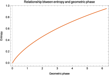
Figure 1: $\gamma_{c}$ is set to vary form $0$ to $2\pi$.

IV Conclusions and Acknowledgements

In this article, the geometric phase factor for two-mode squeezed state is evaluated explicitly. The total phase factor (13) is turned to be an elegant outcome, which is just one term of the product of the initial squeezed operator and final squeezed operator (9). When this system undergoes cyclic evolutions, the corresponding geometric phase is obtained, which is just the sum of the counterparts of two isolated one-mode squeezed state. Furthermore, the relationship between the cyclic geomtric phase and entanglement of two-mode squeezed state is established.

D.B.Y. is supported by NSF of China under Grant No. 11447196. And J.X.H. is supported by the NSF of China under Grant 11304037, the NSF of Jiangsu Province, China under Grant BK20130604, as well as the Ph.D. Programs Foundation of Ministry of Education of China under Grant 20130092120041.

References

- [1] J Anandan. Non-adiabatic non-abelian geometric phase. Physics Letters A, 133(4-5):171–175, 1988.
- [2] M. V. Berry. Quantal phase factors accompanying adiabatic changes. Proceedings of the Royal Society of London. Series A, Mathematical and Physical Sciences, 392:45–57, 1984.
- [3] A Bohm, A Mostafazadeh, H Koizumi, Q Niu, and J Zwanziger. The geometric phase in quantum systems. Springer-Verlag, 2003.
- [4] Carlton M. Caves and Bonny L. Schumaker. New formalism for two-photon quantum optics. i. quadrature phases and squeezed states. Physical Review A, 31(5):3068–3092, 1985. PRA.
- [5] S. Chaturvedi, MS Sriram, and V. Srinivasan. Berry’s phase for coherent states. Journal of Physics A: Mathematical and General, 20:L1071, 1987.
- [6] D. Chruscinski and A. Jamioikowski. Geometric phases in classical and quantum mechanics, volume 36. Birkhauser, 2004.
- [7] L.M. Duan, JI Cirac, and P. Zoller. Geometric manipulation of trapped ions for quantum computation. Science, 292(5522):1695, 2001.
- [8] J.A. Jones, V. Vedral, A. Ekert, and G. Castagnoli. Geometric quantum computation with nmr. Nature, 1999.
- [9] D Kult. Non-abelian generalization of off-diagonal geometric phases. EPL (Europhysics Letters), 78:60004, 2007.
- [10] LC Kwek and D Kiang. Nonlinear squeezed states. JOURNAL OF OPTICS B: QUANTUM AND SEMICLASSICAL OPTICS, 5:383, 2003.
- [11] Jie Liu, Bambi Hu, and Baowen Li. Nonadiabatic geometric phase and hannay angle: A squeezed state approach. Physical Review Letters, 81(9):1749–1753, 1998. PRL.
- [12] Nicola Manini and F. Pistolesi. Off-diagonal geometric phases. Physical Review Letters, 85(15):3067, 2000. Copyright (C) 2010 The American Physical Society Please report any problems to prola@aps.org PRL.
- [13] N. Mukunda, Arvind, S. Chaturvedi, and R. Simon. Bargmann invariants and off-diagonal geometric phases for multilevel quantum systems: A unitary-group approach. Physical Review A, 65(1):012102, 2001. Copyright (C) 2010 The American Physical Society Please report any problems to prola@aps.org PRA.
- [14] N Mukunda and R Simon. Quantum kinematic approach to the geometric phase. i. general formalism. Annals of Physics, 228(2):205–268, 1993.
- [15] S. Pancharatnam. On the phenomenological theory of light propagation in optically active crystals. Proceedings Mathematical Sciences, 43(4):247–252, 1956.
- [16] Joseph Samuel and Rajendra Bhandari. General setting for berry’s phase. Physical Review Letters, 60(Copyright (C) 2010 The American Physical Society):2339, 1988. PRL.
- [17] Bonny L. Schumaker and Carlton M. Caves. New formalism for two-photon quantum optics. ii. mathematical foundation and compact notation. Physical Review A, 31(5):3093–3111, 1985. PRA.
- [18] Bonny L. Schumaker and Carlton M. Caves. New formalism for two-photon quantum optics. ii. mathematical foundation and compact notation. Physical Review A, 31(5):3093–3111, 1985. PRA.
- [19] A Shapere and F Wilczek. Geometric phases in physics. 1989.
- [20] K. Singh, D. M. Tong, K. Basu, J. L. Chen, and J. F. Du. Geometric phases for nondegenerate and degenerate mixed states. Physical Review A, 67(3):032106, 2003. Copyright (C) 2011 The American Physical Society Please report any problems to prola@aps.org PRA.
- [21] Sj, ouml, Erik qvist, Arun K. Pati, Artur Ekert, Jeeva S. Anandan, Marie Ericsson, Daniel K. L. Oi, and Vlatko Vedral. Geometric phases for mixed states in interferometry. Physical Review Letters, 85(14):2845, 2000. Copyright (C) 2010 The American Physical Society Please report any problems to prola@aps.org PRL.
- [22] D. M. Tong, Sj, ouml, E. qvist, L. C. Kwek, and C. H. Oh. Kinematic approach to the mixed state geometric phase in nonunitary evolution. Physical Review Letters, 93(8):080405, 2004. Copyright (C) 2010 The American Physical Society Please report any problems to prola@aps.org PRL.
- [23] SJ Van Enk. Discrete formulation of teleportation of continuous variables. Physical Review A, 60(6):5095, 1999.
- [24] D.F. Walls. Squeezed states of light. Nature, 306:141–146, 1983.
- [25] F Wilczek and A Zee. Appearance of gauge structure in simple dynamical systems. Physical Review Letters, 52(24):2111–2114, 1984.
- [26] Di Xiao, Ming-Che Chang, and Qian Niu. Berry phase effects on electronic properties. Reviews of Modern Physics, 82(3):1959–2007, 2010. RMP.
- [27] A. Anandan Y.Aharonov. Phase change during a cyclic quantum evolution. Phys. Rev. Lett, 58(1593), 1987.
- [28] D.B. Yang, Y. Chen, F.L. Zhang, and J.L. Chen. Geometric phases for nonlinear coherent and squeezed states. Journal of Physics B: Atomic, Molecular and Optical Physics, 44:075502, 2011.