Abstract

Large spatial datasets often represent a number of spatial point processes generated by distinct entities or classes of events. When crossed with covariates, such as discrete time buckets, this can quickly result in a data set with millions of individual density estimates. Applications that require simultaneous access to a substantial subset of these estimates become resource constrained when densities are stored in complex and incompatible formats. We present a method for representing spatial densities along the nodes of sparsely populated trees. Fast algorithms are provided for performing set operations and queries on the resulting compact tree structures. The speed and simplicity of the approach is demonstrated on both real and simulated spatial data.

1 Introduction and motivation

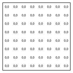
(a) $m^{0}=0$

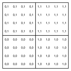
(b) $m^{0}=1$

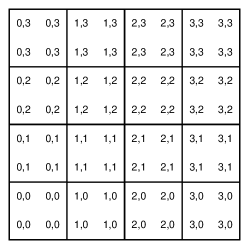
(c) $m^{0}=2$

Figure 1: Partitioning of a $2^{3}$ by $2^{3}$ grid into quadtree based groups. The pair of numbers printed on each grid point represent the corrisponding $m^{1}$ and $m^{2}$ coordinates. Note that there is one final set of partitions for $m^{0}=3$, where each point is in its own tile.

Many large streaming datasets are generated by systems that continually record the location of spatially-centric events. Examples include the address where ambulances are requested through an emergency dispatch center, location names detected in a query through a web search engine, and the GPS coordinates recorded by a taxicab’s routing software. When spatial measurements come from a relatively small and discrete set, they can often be handled just like any other covariate. Spatial data recorded from a very large set, such as addresses, or as a continuous measurement of latitude and longitude, may require more specialized treatment. Predicting the location of the next observation, for example, is often accomplished by modeling historical data as a spatial point process and estimating a density function with techniques such as kernel density estimators or Gaussian mixtures.

With enough data, it may be both possible and desirable to generate alternative density estimates for different classes of events. When crossing several variables, densities can quickly become quite granular; consider, for example,the density of ambulance requests ‘related to traffic accidents from 7am-8am on Tuesdays’. An increase in granularity comes with a corresponding increase in the number of density estimates that must be stored. On its own, this increase is not a particular point of concern. The estimates can be stored in an off-the-shelf database solution, a small subset relevant to a given application can be queried, and the results used in a standard fashion.

Computational issues do arise when there is a need to simultaneously work with a large set of densities. Inverse problems, where an event is detected in a location and the type of event must be predicted, present a common examples of such an application. Performing set operations, such as intersections and unions, to construct even more complex density estimates is another example. A large set of non-parametric density estimates, represented by predictions over a fine-grained lattice, can lead to a substantial amount of memory consumption. Parametric estimates, perhaps compactly represented by Gaussian mixtures, may be safely loaded into memory but eventually cause problems as set operations between densities yield increasingly complex results. These make inference and visualization intractable as the scale of the data increases.

As a solution to these problems, we present a method that combines the benefits of parametric and non-parametric density estimates for large spatial datasets. It represents densities as a sum of uniform densities over a small set of differently sized tiles, thus yielding a sparse representation of the estimated model. At the same time, the space of all possible tiles is a relatively small and fixed set; this allows multiple densities to be aggregated, joined, and intersected in a natural way. By using a geometry motivated by quadtrees we are also able to support constant time set operations between density estimates.

2 Prior work

The estimation of general density estimation has a long history, with many spatial density routines being a simple application of generic techniques to the two-dimensional case. Mixture models were studied as early as 1894 by Karl Pearson [14], with non-parametric techniques, such as kernel density estimation, being well known by at least the 1950s [13], [16]. Further techniques have also been developed in the intervening years, such as smoothed histograms [10], splines [2, 5], Poisson regression [5], and hierarchical Bayes [19]. A variant on mixture models that allow for densities to depend on additional covariates was proposed by Schellhase and Kauermann [18], though their work focuses only on one-dimensional models.

Computational issues regarding density estimation have also been studied in the recent literature. Some attention has focused on calculating the kernel density estimates given by a large underlying training dataset [15, 22]. As an active area of computer vision, there as been a particular interest on two-dimensional problems [4, 20, 23]. These often utilize some variation of the fast Gauss transform of Greengard and Strain [9]. To the best of our knowledge, no prior work has focused on the computational strains of working simultaneously with a large set of density estimates.

A significant amount of literature and software also exists from the perspective of manipulating generic spatial data within a database. These store spatial data in a format optimized for some set of spatial queries, such as k-nearest neighbors or spatial joins [21], and can be made to handle and query fairly large sets of data. Recent developments have even made spatial queries possible over data distributed across horizontally scalable networks [12], and integrated for fast real-time visualizations [11]. The elements in such systems are typically points, lines, or polygons. Density functions can be encoded into such a system by storing the centroid of the density modes within mixture models, or saving predictions over a fine grid for non-parametric models. The problem in using this solution for our goal is that operations on the parametric models do not translate into fast queries on the database, and the size of the grid required to store non-parametric models quickly grows prohibitively large. Our solution builds a density estimate that can be queried within a database system, but stored in a significantly smaller space.

3 Density estimation

3.1 Approach

For the remainder of this article, we focus on density estimation over a rectangular grid of points. We assume that there is some observed sample density $y_{i}$ over the grid, which generally corresponds to assigning observations to the nearest grid point, and an initial estimate of the density given by $z_{i}$. The latter typically comes from a kernel density estimate, but may be generated by any appropriate mechanism. Our goal is to calculate predictions $x_{i}$ such that the following are all true:

1. The new estimates are expected to be nearly equally as predictive for a new set of observed data $y_{new}$ as the estimates $z_{i}$,

   $$\mathbb{E}||y_{new}-z||\approx\mathbb{E}||y_{new}-x||$$ (1)

2. The estimates $x_{i}$ can be represented as a sparse vector over some fixed dictionary $\mathcal{D}$, which has a total dimension of size $\mathcal{O}(n)$, the number of data points in the grid.

3. Queries of the form $\sum_{i\in A}x_{i}$ can typically be calculated faster than $\mathcal{O}(|A|)$ for $A$ corresponding to any subset of points over the original grid.

To satisfy these requirements, we construct an over-complete, hierarchical dictionary and calculate an estimate of $z$ using an $\ell_{1}$-penalized regression model.

3.2 Quadtree dictionary

In order to describe our target dictionary, it is best to consider the case where the grid of points is a square with $2^{k}$ points on each side. We otherwise embed the observed grid in the smallest such square and proceed as usual knowing that we can throw away any empty elements in the final result.

For any integer $m^{0}$ between $0$ and $k$, we define the following sets:

$$\mathcal{T}^{m^{0}}_{m1,m2} =\left\{i:\left\lfloor\frac{i\,(\text{mod}\,2^{k})}{2^{m^{0}}}\right\rfloor=m_{1},\left\lfloor\frac{i}{2^{k+m^{0}}}\right\rfloor=m_{2}\right\}$$

$$\forall \,m^{1},m^{2}\in\left\{0,1,\ldots,2^{m^{0}}-1\right\}$$ (2)

For a fixed $m^{0}$, these sets produce a disjoint, equally sized, partition of the grid of points, with $m^{1}$ and $m^{2}$ giving the horizontal and vertical coordinates of the superimposed grid. We refer to each $\mathcal{T}^{m^{0}}_{m1,m2}$ as a tile, as it represents a square subset of the original lattice. For a visualization of the partitioning scheme over a small grid, see Figure 1. It will be helpful to have a way of referencing the set of all tiles that share a given $m^{0}$ parameter, often referred to as a zoom level:

$$\mathcal{T}^{m^{0}} =\left\{\mathcal{T}^{m^{0}}_{m1,m2},\,\text{s.t.}\,m^{1},m^{2}\in\left\{0,1,\ldots,2^{m^{0}}\right\}\right\}$$ (3)

Combining all of the zoom levels, we can construct the set of all tiles from which we will define the final dictionary:

$$\mathcal{T} =\bigcup_{m^{0}=0}^{k}\mathcal{T}^{m^{0}}$$ (4)

We will assume that there is some fixed order of this set, so that we may refer unambiguously to the $j$-th tile $\tau_{j}$ in the set $\mathcal{T}$. The elements $m^{0}_{j}$, $m^{1}_{j}$, and $m^{2}_{j}$ refer to the corresponding indices of that $j$-th tile. The set $\mathcal{T}$ consists of all tiles corresponding to a fixed depth quadtree over the grid of all points. They mirror the structure of tiles used in tilemap servers, such as slippy map generated by OpenStreetMap [17]. When the grid is defined over the entire globe, our tiles directly coincide with the slippy tiles.

Finally, we define the dictionary $D^{\alpha}$ as a sparse matrix in $\mathbb{R}^{4^{k}\times d}$, with $d=|\mathcal{T}|$. It is defined such that:

$$D_{i,j}^{(\alpha)} =\begin{cases}4^{-m^{0}_{j}\cdot\alpha},&\text{if }x_{i}\in\tau_{j}\\ 0,&\text{otherwise}\end{cases}$$ (5)

For $\alpha$ equal to $1$, element $D_{i,j}^{(1)}$ encodes the proportion of the tile $\tau_{j}$ that is covered by the point $x_{i}$. The element $D_{i,j}^{(0)}$ is instead a simple indicator for whether a the point $x_{i}$ is in tile $\tau_{j}$. Other values of $\alpha$ provide a continuous scale of weightings to the tiles that moves between these two extremes, and will be useful in the penalized estimation routine. Notice that the dictionary is an over-representation of the space of all possible estimators, and for $\alpha$ equal to $0$, contains a copy of the identity matrix as a permuted subset of its columns.

3.3 Estimation algorithm

In order to learn a sparse representation of $z$ given our dictionary $D^{\alpha}$, we first use an $\ell_{1}$-penalized estimator. This well-known technique produces a parsimonious estimator via convex optimization. The parameter $\alpha$ is set to a number between $0$ and $1$ to control the degree to which the penalty should be proportional to tile size. A large parameter will yield a model with many small tiles, whereas a small parameter gives a smaller model with more large tiles. We find that a value near $0.5$ typically works well.

$$\widehat{b^{1}} =\mathop{\mathrm{arg\,min}}_{b}\left\{||z-D^{(\alpha)}b||_{2}^{2}+\lambda\cdot||b||_{1}\right\}$$ (6)

In order to solve Equation 6, we calculate the regularization path for a sequence of $\lambda$ values using software that provides a customized application of coordinate decent [8]. Choosing the final tuning parameter can be done by a number of methods; we have found the one standard deviation rule, originally suggested by Breiman, with 5-fold cross validation provides good predictability without overfitting the model [3].

To increase interpretability and reduce prediction bias, we calculate the non-negative least squares estimator over the support of the $\ell_{1}$-penalized estimator. With a large training dataset, this should be refit on a holdout set. Empirically, we observe good performance even when refitting on the same training data. Without the $\ell_{1}$-penalty the choice of $\alpha$ does not effect the predicted values, so here we use $D^{1}$ to facilitate the interpretability and normalization of the results.

$$\widehat{b^{2}}=\mathop{\mathrm{arg\,min}}_{b} \left\{||z-D^{(1)}b||_{2}^{2}\quad\text{s.t.}\right.$$

$$\quad\left.\text{supp}(b)=\text{supp}(\widehat{b^{1}})\quad\text{and}\quad b_{j}\geq 0\right\}$$

We then hard threshold the non-negative least squares solution by a value of $\delta$.

$$\widehat{b^{3}}_{j} =\begin{cases}\widehat{b^{2}_{j}},&\text{if }\widehat{b^{2}_{j}}>\delta\cdot||\widehat{b^{2}}||_{1}\\ 0,&\text{otherwise}\end{cases}$$ (7)

And finally, the density estimator is normalized to have a sum of $1$:

$$\widehat{b} =\frac{\widehat{b^{3}}}{||\widehat{b^{3}}||_{1}}$$ (8)

The predicted values, $x$, can be calculated by projecting $\widehat{b}$ by the dictionary $D^{(1)}$.

$$x =D^{(1)}\widehat{b}$$ (9)

Clearly we do not want to save the predicted values explicitly. Otherwise, we would have simply saved the raw predicted values $z$. We instead show, in the next subsection, that predictions $x$ can be generated quickly from the sparse vector $\widehat{b}$.

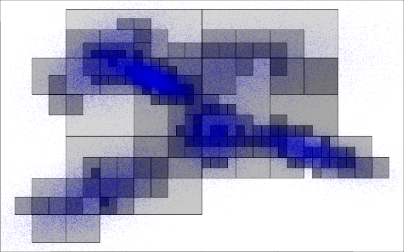
Figure 2: Scatter plot of the training data from the simulated Gaussian mixture model superimposed over the predicted densities from tile model with grid size equal to $4^{7}$ and $\alpha$ equal to $0.8$.

num.	$\alpha$ parameter									$\bar{y}$
tiles	0	0.1	0.25	0.33	0.5	0.66	0.75	0.9	1
$4^{3}$	0.662	0.662	0.566	0.566	0.714	0.714	0.454	0.714	0.809	0.137
$4^{4}$	0.177	0.266	0.266	0.266	0.200	0.148	0.147	0.808	0.808	0.134
$4^{5}$	0.212	0.211	0.210	0.202	0.189	0.195	0.198	0.914	0.974	0.178
$4^{6}$	0.267	0.258	0.241	0.239	0.242	0.250	0.252	0.263	0.979	0.217
$4^{7}$	0.320	0.322	0.308	0.307	0.312	0.315	0.319	0.338	0.989	0.289

Table 1: Total variation distance of predicted model to the true model from a Gaussian mixture with 6 modes. Results are shown for varying $\alpha$ and grid sizes. The total variation of the simple histogram (i.e., $\bar{y}$) estimator is shown for comparison.

num.	$\alpha$ parameter
tiles	0	0.1	0.25	0.33	0.5	0.66	0.75	0.9	1
$4^{3}$	1	1	3	3	2	2	4	2	1
$4^{4}$	33	15	15	15	24	48	48	3	3
$4^{5}$	59	63	76	105	128	128	128	2	1
$4^{6}$	63	87	144	161	198	174	182	198	0
$4^{7}$	66	87	145	167	199	167	168	171	6

Table 2: Number of tiles with non-zero weights for the predicted model over the simulated Gaussian mixture with 6 modes. Results are shown for varying $\alpha$ and grid sizes, and use a constant $\delta$ equal to $0.001$.

3.4 Fast query techniques

Given the quadtree nature of dictionary $D$, any particular grid point $x_{i}$ is represented by at most $k+1=\log_{4}(n)+1$ elements. This implies that we can calculate the predicted value at that point in $\mathcal{O}(\log(n))$ time. Due to the nature of the $\ell_{1}$-penalty, the number of non-zero terms of $\widehat{\beta}$ should be small; we denote this by $||\widehat{\beta}||_{0}=s$. Given the hardthresholding in our example, $s$ is at most $\delta^{-1}$ but will typically be much smaller. From this it is possible to calculate $\sum_{i\in A}x_{i}$ in $\mathcal{O}(s\log(n))$ time.

Assume now that we have two estimates density estimates, $\widehat{b}_{A}$ and $\widehat{b}_{B}$, which represent the densities $\mathbb{P}(x_{i}|A)$ and $\mathbb{P}(x_{i}|B)$ for disjoint events $A$ and $B$. In order to estimate $\mathbb{P}(x_{i}|A\cup B)$, we can take the weighted sum of their sparse representations:

$$\widehat{b}_{A\cup B} =\mathbb{P}A\cdot\widehat{b}_{A}+\mathbb{P}B\cdot\widehat{b}_{B}$$ (10)

The final representation may be further hard thresholded by $\delta$ to guarantee that $\widehat{b}_{A\cup B}$ has no more than $\delta^{-1}$ elements. We can analogously use the same method to take the union of an large set of densities.

Finally, consider observing two independent samples in which we first observe event $A$ and then observe the event $B$. Conditioned on the fact that both were observed in the same location, we wish to calculate the density over space given the estimators $\mathbb{P}(x_{i}|A)$ and $\mathbb{P}(x_{i}|A)$. We call the event of observing $A$ followed by $B$ in the same location‘ $C$’. Applications of this type of event arise when a single person or device is observed displaying two types of events in close temporal proximity to one another (in other words, too fast to have moved given the granularity of the grid).

We cannot directly calculate this density of the non-zero elements of the sparse estimators, however clearly we have the following relationship between the sparse representations:

$$D^{(1)}\widehat{b}_{C} =D^{(1)}\widehat{b}_{A}\cdot D^{(1)}\widehat{b}_{B}$$ (11)

Calculating this directly would require computing estimates of the original densities at all $n$ grid points. However, notice that because of the hierarchical structure of the dictionary, $D^{(1)}\widehat{b}_{A}$ has at most $||\widehat{b}_{A}||_{0}+1$ unique values. This is due to the fact that for any two tiles either one contains the other or they are disjoint. Likewise, the product $D^{(1)}\widehat{b}_{A}\cdot D^{(1)}\widehat{b}_{B}$ has at most $||\widehat{b}_{A}||_{0}+||\widehat{b}_{B}||_{0}+1$ unique values. Therefore the unique values of the right hand side of Equation 11 can be calculated in $\mathcal{O}(s)$ time. Similarly $\widehat{b}_{C}$ can be solved for in $\mathcal{O}(s)$ time because it is known that the solution lies in the joint support of $\widehat{b}_{A}$ and $\widehat{b}_{B}$.

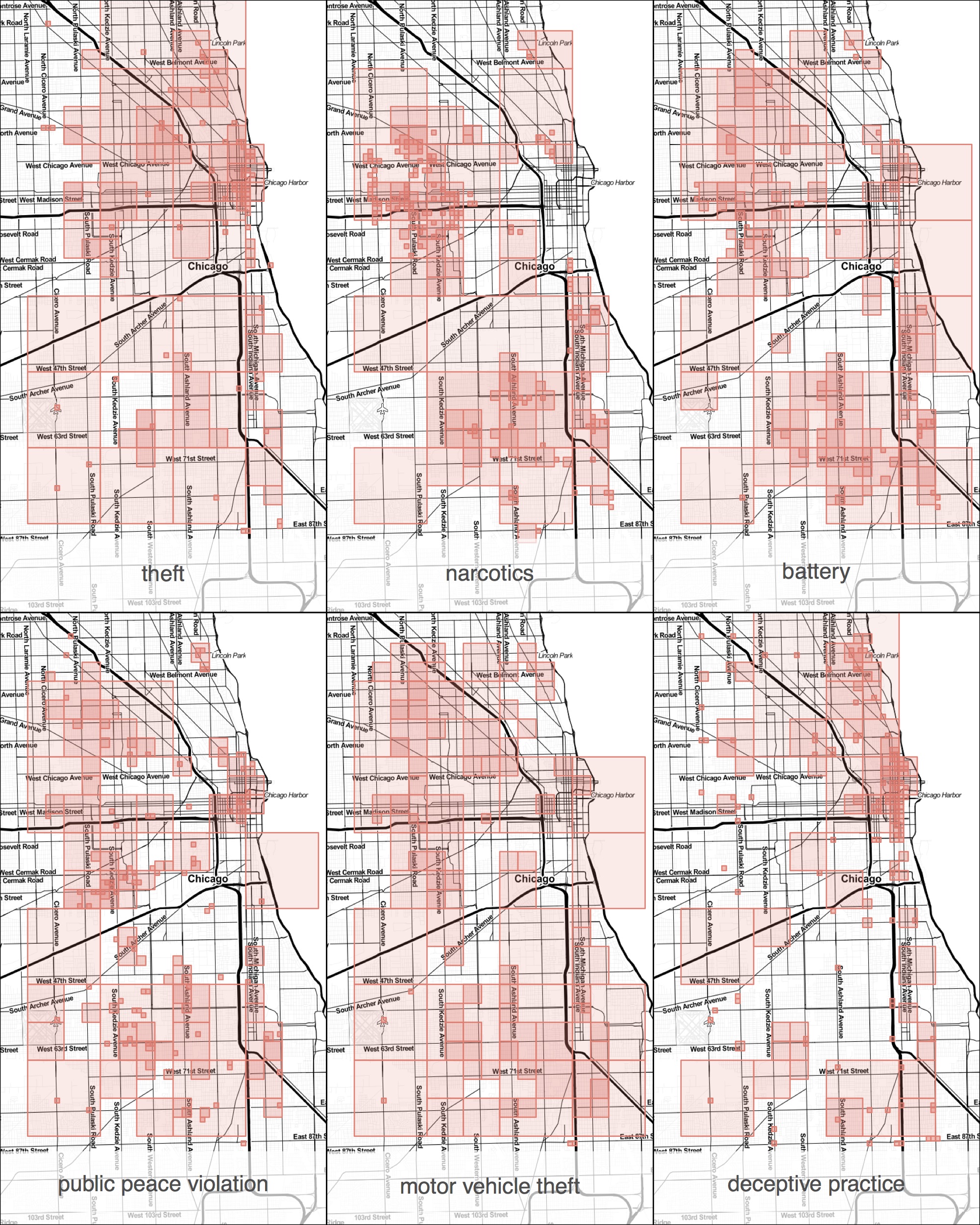
Figure 3: Six predicted models for the spatial density of the occurance of six times of crimes in the Chicago crime sataset. The $\alpha$ parameter is fixed to be $0.4$ across all models. Map tiles by Stamen Design.

					peace	vehicle	deceptive
		theft	narcotics	battery	violation	theft	practice
	theft	143	226	210	195	154	171
	narcotics		239	241	254	219	257
	battery			156	226	195	244
	peace violation				191	197	228
Union	vehicle theft					107	187
	deceptive practice						186
	theft	143	227	190	199	157	188
	narcotics		231	266	287	246	151
	battery			152	218	157	168
	peace violation				174	197	166
	vehicle theft					106	168
Intersection	deceptive practice						173

Table 3: Number of non-zero tile weights in the Chicago crime data, for pairwise unions and intersections with $\alpha=0.4$ and $\delta=0.001$. Note that self-unions return the original density.

	start hour
stop hour	00	02	04	06	08	10	12	14	16	18	20	22
02	189	174	184	189	188	179	171	175	168	166	161	163
04		196	187	199	191	182	170	167	165	163	164	162
06			208	190	188	188	175	166	164	161	158	158
08				230	199	185	171	167	160	157	160	161
10					210	166	160	160	158	157	157	156
12						188	162	160	163	165	158	153
14							183	161	170	160	154	158
16								187	173	160	160	162
18									194	159	163	164
20										175	159	166
22											190	170
24												197

Table 4: The number of non-zero coefficients attained by taking the union of contiguous ranges from the two-hour (local time) Uber pickup densities. All combinations of inter-day ranges (that is, not crossing midnight) between even hours are shown. All hours are in local time.

	start hour
stop hour	00	02	04	06	08	10	12	14	16	18	20	22
02	201	223	256	259	250	243	217	180	150	116	84	45
04		194	273	292	276	261	257	230	190	150	108	62
06			208	266	259	251	245	227	186	146	97	62
08				228	256	256	250	244	214	182	167	119
10					208	243	231	224	215	174	170	152
12						188	203	195	190	175	172	167
14							183	203	196	191	188	177
16								187	203	197	206	193
18									195	211	222	226
20										176	214	221
22											190	224
24												198

Table 5: The number of non-zero coefficients attained by taking the intersection of contiguous ranges from the two-hour (local time) Uber pickup densities. All combinations of inter-day ranges (that is, not crossing midnight) between even hours are shown. All hours are in local time.

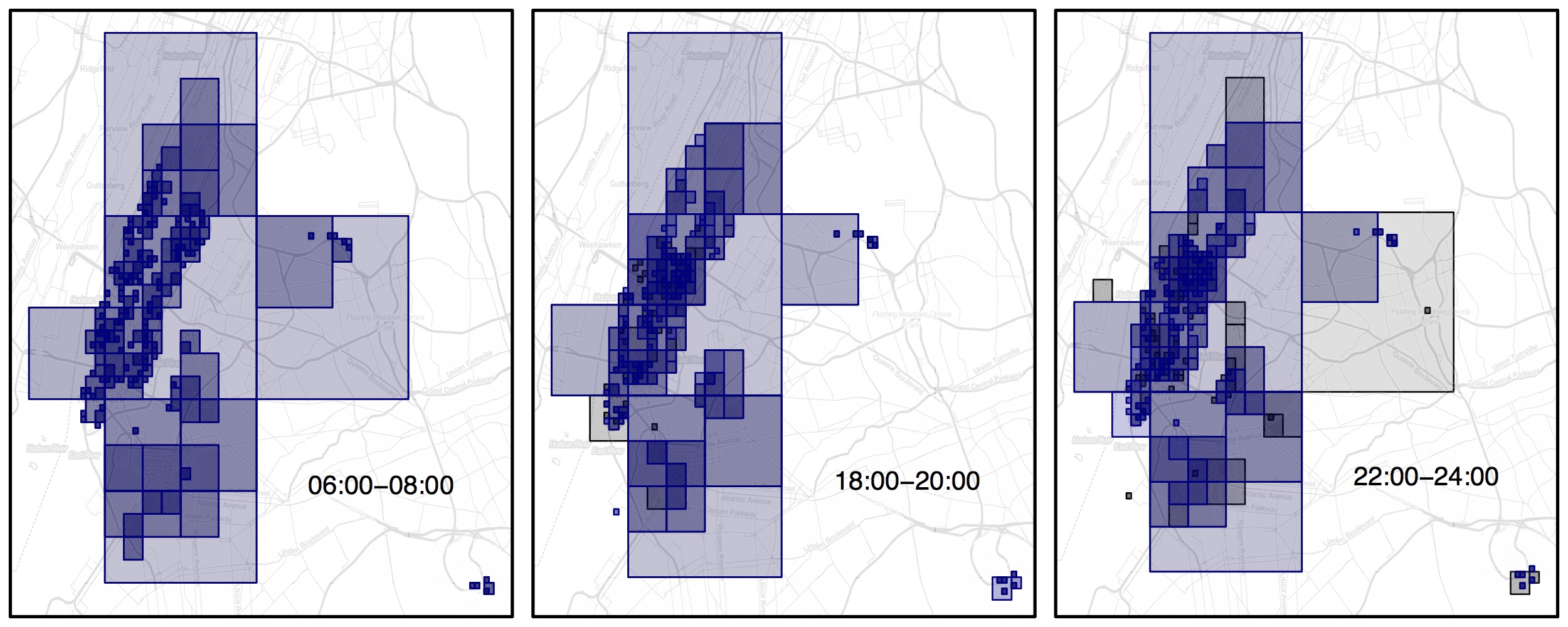
Figure 4: Three predicted models for the spatial density of the Uber pickup location dataset for two hour intervals. The $\alpha$ parameter is fixed to be $0.4$. All hours are in local time. Map tiles by Stamen Design.

4 Simulation from a Gaussian mixture model

We sampled a set of two hundred thousand points from a Gaussian mixture model with $6$ modes. Using $\delta=0.001$, we calculated the sparse representation of the density over the quadtree based dictionary. A scatterplot of the sampled points superimposed over the predicted densities are shown in Figure 2 for a particular grid size and value of $\alpha$. Table 1 displays the total variation distance between the estimated density and the true Gaussian distribution over a grid of tile sizes and values of $\alpha$. These are compared to the total variation distances gained by directly using the observed densities at each point. We see that, with the exception of the smallest grid size, the total variation of both estimators performs more poorly with larger grid sizes. This seems reasonable as larger grid sizes provide a harder estimation problem with many more degrees of freedom. The total variation as a function of $\alpha$ shows that values too close to $1$ perform poorly regardless of the grid size. Values near $0$ function okay, but the optimal value tends to be from $0.25$ to $0.75$.

In Table 2, we show the number of non-zero elements in the prediction vector by grid size and the $\alpha$ parameter. The number of non-zero elements generally increases with the grid size. Given the exponentially growing dictionary size this is not surprising, however it is interesting that the sizes do not grow exponentially. This shows the ability of our method to represent complex, granular densities in a relatively compact way regardless of the grid size. When $\alpha$ is equal to $1$ (or very close to it) the predicted model size is very small. This is the result of a poor model fit due to overfitting on small tile sizes; the cross-validation procedure eliminates the overfitting and leaves a relatively constant model. We recommend setting $\alpha$ to anything between $0$ and the value that maximized the model size. In this simulation notice that maximizing the model size with respect to $\alpha$ would generate the lowest total variation of the resulting model. This is a useful heuristic because while Table 1 cannot be generated without knowing the true generating distribution, Table 2 can be created without an external information.

5 Applications

5.1 Chicago crime data

The city of Chicago releases incident level data for all reported crimes that occur within the city [1]. We fit sparse density estimates to six classes of crimes; these estimated densities are shown in Figure 3. We have picked classes that exhibit very different spatial densities over the city. For example, deceptive practice crimes occur predominantly in the center of the city whereas narcotics violations are concentrated in the western and southern edges of Chicago. Table 3 shows the number of non-zero terms in the predicted density vectors of pairwise unions and intersections. Of particular importance, note that the complexity of the unions and intersections are not significantly larger than the complexity of the original estimates (given by diagonal terms of the table of unions). This property would not hold for most other density estimation algorithms.

5.2 Uber pickup locations in NYC

In response to a freedom of information request, the New York City government released a dataset showing the requested pickup locations from $5$ million rides commissioned by the transit company Uber [7]. We used this data to construct two-hour density buckets, three of which are shown in Figure 4. Notice that, unlike the Chicago crime data, the non-zero tiles are relatively consistent from image to image, roughly following the population density of the city. Temporal differences do exist: for example the heavily neighborhood of the Upper West Side has a particularly high density only during the morning commute. The ability to detect localized spikes at the airports exhibit the adaptive nature of the sparse learning algorithm.

Table 4 shows the model sizes when computing the union of densities from any continuous time interval during the day. Due to the truncating of small densities by $\delta$ and the fact that the non-zero tiles generally line up across time periods, the overall size of the unions never grows much larger than the original estimates. Table 5 shows the same information over arbitrary unions. These intersections would be useful, for example, when trying to determine where taxicab waiting spots should be constructed as they indicate areas of high density throughout periods of the day.

Overall, we are able to quickly calculate $144$ complex densities by only estimating and storing $12$ of them (or $4095$, when considering non-contiguous time periods).

6 Conclusions and future extensions

We have presented an algorithm for calculating sparse representations of spatial densities. This method has been shown to be able to compute fast density estimations over arbitrary regions and to support union and intersections over a large set of independent density estimates. These claims have been illustrated theoretically, by controlled simulations, and over two real datasets. We are now looking to generalize the quadtree approach to work with alternative hierarchical partitions of space. In particular, this could create a finer grained dictionary near places of high density (i.e., roads and city centers) allowing for a smaller dictionary and further decreasing the estimation error.

References

References

- [1] Crimes: 2001 to present. https://data.cityofchicago.org/. Accessed: 2015-04-30.
- [2] Liliana I Boneva, David Kendall, and Ivan Stefanov. Spline transformations: Three new diagnostic aids for the statistical data-analyst. Journal of the Royal Statistical Society. Series B (Methodological), pages 1–71, 1971.
- [3] Leo Breiman. Better subset regression using the nonnegative garrote. Technometrics, 37(4):373–384, 1995.
- [4] E Cruz Cortés and Clayton Scott. Sparse approximation of a kernel mean. arXiv preprint arXiv:1503.00323, 2015.
- [5] Paul HC Eilers and Brian D Marx. Flexible smoothing with b-splines and penalties. Statistical science, pages 89–102, 1996.
- [6] Ahmed Elgammal, Ramani Duraiswami, and Larry S Davis. Efficient kernel density estimation using the fast gauss transform with applications to color modeling and tracking. Pattern Analysis and Machine Intelligence, IEEE Transactions on, 25(11):1499–1504, 2003.
- [7] Andrew Flowers. Uber trip data from a freedom of information request to nyc’s taxi & limousine commission. https://github.com/fivethirtyeight/uber-tlc-foil-response, 2015.
- [8] Jerome Friedman, Trevor Hastie, and Rob Tibshirani. Regularization paths for generalized linear models via coordinate descent. Journal of statistical software, 33(1):1, 2010.
- [9] Leslie Greengard and John Strain. The fast gauss transform. SIAM Journal on Scientific and Statistical Computing, 12(1):79–94, 1991.
- [10] Chong Gu and Jingyuan Wang. Penalized likelihood density estimation: Direct cross-validation and scalable approximation. Statistica Sinica, 13(3):811–826, 2003.
- [11] Lauro Lins, James T Klosowski, and Carlos Scheidegger. Nanocubes for real-time exploration of spatiotemporal datasets. Visualization and Computer Graphics, IEEE Transactions on, 19(12):2456–2465, 2013.
- [12] Jan Kristof Nidzwetzki and Ralf Hartmut Güting. Distributed secondo: A highly available and scalable system for spatial data processing. In Advances in Spatial and Temporal Databases, pages 491–496. Springer, 2015.
- [13] Emanuel Parzen. On estimation of a probability density function and mode. The annals of mathematical statistics, pages 1065–1076, 1962.
- [14] Karl Pearson. Contributions to the mathematical theory of evolution. Philosophical Transactions of the Royal Society of London. A, pages 71–110, 1894.
- [15] Vikas C Raykar, Ramani Duraiswami, and Linda H Zhao. Fast computation of kernel estimators. Journal of Computational and Graphical Statistics, 19(1):205–220, 2010.
- [16] Murray Rosenblatt et al. Remarks on some nonparametric estimates of a density function. The Annals of Mathematical Statistics, 27(3):832–837, 1956.
- [17] John T Sample and Elias Ioup. Tile-based geospatial information systems: principles and practices. Springer Science & Business Media, 2010.
- [18] Christian Schellhase and Göran Kauermann. Density estimation and comparison with a penalized mixture approach. Computational Statistics, pages 1–21, 2012.
- [19] Daniel AM Villela, Claudia T Codeço, Felipe Figueiredo, Gabriela A Garcia, Rafael Maciel-de Freitas, and Claudio J Struchiner. A bayesian hierarchical model for estimation of abundance and spatial density of aedes aegypti. 2015.
- [20] Changjiang Yang, Ramani Duraiswami, Nail Gumerov, Larry Davis, et al. Improved fast gauss transform and efficient kernel density estimation. In Computer Vision, 2003. Proceedings. Ninth IEEE International Conference on, pages 664–671. IEEE, 2003.
- [21] Albert KW Yeung and G Brent Hall. Spatial database systems: Design, implementation and project management, volume 87. Springer Science & Business Media, 2007.
- [22] Yan Zheng, Jeffrey Jestes, Jeff M Phillips, and Feifei Li. Quality and efficiency for kernel density estimates in large data. In Proceedings of the 2013 ACM SIGMOD International Conference on Management of Data, pages 433–444. ACM, 2013.
- [23] Yan Zheng and Jeff M Phillips. L- error and bandwidth selection for kernel density estimates of large data. In Proceedings of the 21th ACM SIGKDD International Conference on Knowledge Discovery and Data Mining, pages 1533–1542. ACM, 2015.