A Recipe for Composite Materials: An Approach through Fiber Bundle Model
Abstract
Strengthening of materials and preventing abrupt fracture are really challenging jobs in the field of engineering and material science. Such problems can be resolved by using composite materials. In this work, we have studied the fracture process of a composite material in light of fiber bundle model with different elastic constants as well as different random threshold breaking strength of fibers. The critical width of the threshold distribution (), for which abrupt failure occurs, is studied both analytically and numerically with increasing number of components in the composite and it is shown that is inversely related to . Corresponding phase diagram for the model suggests decrease in the tendency of abrupt fracture as number of components in the composite increase.
pacs:
62.20.mm, 62.25.Mn, 46.50.+a, 81.40.NpFracture and material stability attracted human being from long time back when they started using materials found in nature to serve their own purposes. Fracture in materials is a complex phenomenon which involves very large length and time scales. The first scientific approach to realize the strength of materials was by Leonardo da Vinci Lund , followed by Galileo Galilei and Edme Mariotte. During the last 25 years, fracture problems has been revisited by physicists Chak1 ; Herrmann ; Kawa . Fracture in materials are mainly guided by either extreme events or collective behavior of the cracks present in the material. In the later case, the material shows deformation in form of precursory rupture events prior to global failure. However, in the first case, a sharp crack, mostly the weakest one, spans the total length of the material denoting global failure without showing any precursory events. This behavior is disadvantageous for industrial purpose. This problem can be resolved to some extent by the introduction of composite materials where materials of different mechanical and chemical properties are mixed to form a new material. The composite material usually comes with either greater strength or with less risk of abrupt failure compared to its components brian ; Luigi . Example of such composites are cements, concrete, metal composites, ceramic composites etc.
Fiber Bundle Model (FBM) is an important but simple model to study fracture-failure phenomena. This model is able to mimic correctly the avalanche behavior of fracture in materials Chak2 . It was first introduced by Pierce Pierce . The FBM consists of fibers or Hookean springs, attached between two parallel plates. The plates are pulled apart by a force which exerts stresses on fibers. Once the stress crosses the breaking threshold of a particular fiber, chosen from a random distribution, the fiber breaks. There are two varieties of the FBM, equal load sharing FBM (ELS) and local load sharing FBM (LLS). For the ELS Pierce ; Daniels no local deformation and hence no stress concentration occur anywhere around the failed fibers and the stress of the failed fibers is shared among all surviving fibers democratically. The load per fiber therefore increases initiating failure of more fibers and so on. On the other hand, in LLS Phoenix1 ; Phoenix2 ; Phoenix3 ; Harlow1 ; Harlow2 ; Harlow3 , the terminal stress of a failed fiber is equally shared only among its nearest surviving neighbors.
In this paper, we have studied the fracture process of a composite bundle containing fibers of different elasticities with certain probabilities in the framework of fiber bundle model under ELS scheme. In kun2 ; kun3 , the authors considered a fiber bundle model where a fraction are unbreakable and the remaining fibers are weak and have randomly distributed failure strength. The brittle to ductile transition was shown at a critical value of this fraction . In our model, there is no such unbreakable fraction of fibers. Here, inhomogeneity is introduced in terms of elastic modulus of the fibers. In case of a bundle having -components, the elasticities of individual components are chosen between two extreme values and with spacing and probability . In a previous work, Kun a system with continuously varying Young’s modulus and with a constant breaking strength was studied. However, in our model, elasticity is not the only source of disorder but also the threshold strength () of fibers is. Here, the fibers have different thresholds chosen within the window to of the uniform distribution where is the threshold stress corresponding to weakest link of the chain of fibers and is the half width of the distribution. Each fiber has a local elastic modulus . A strain , same everywhere in the bundle, is applied externally. The load on the bundle at this condition is , where . The breaking condition is which depends both on elasticities and breaking thresholds. In this way we can say that fibers break when the externally applied strain crosses its local strain threshold . After breaking of those fibers the strain is to be redistributed over the remaining fibers in equal amount keeping total stress constant. This may induce breaking of more fibers as the strain on the bundle gets increased. At low values, the rupturing of the weakest fiber may result in failure of the entire system. However, at large values, for the initial applied strain, the system will reach a stable point where no further rupture of fibers is possible as the next minimum strain threshold is above the redistributed strain. For further rupture, we have to increase the external strain by a little amount, so that the breaking condition is satisfied. Thus the system will go through a series of stable states in succession of avalanches of rupturing of fibers till the critical strain is reached that can cause failure of the remaining fibers.
For analytical calculations, first we have chosen the 2-component system. If now the system suffers from a strain , the average stress of the system will be: , where , are elasticities of fibers of type 1 and type 2 respectively and are stresses on type 1 and type 2 fibers respectively. At a certain point of this dynamics if fraction of type 1 and fraction of type 2 fibers are broken, then the redistributed strain on the remaining fibers is
| (1) |
Thus all fibers (type 1 and type 2) having breaking thresholds below will fail.
The corresponding stress on type , i.e., is given by,
| (2) |
where or .
Broken fraction of type fibers will be
| (3) |
where or corresponding to the type of fibers and is the strain threshold distribution. In terms of threshold stress distribution we have,
| (4) |
where is the uniform threshold distribution. Using Eq. 2 into Eq. 4 we get two quadratic equations for and . Solving the quadratic equations we get the solutions for fraction of broken bonds as :
| (5) |
where and .
At critical point the solution becomes,
| (6) |
Then total fraction broken at critical point for a particular width of disorder () will be given as
| (7) |
Then fraction unbroken at critical point will be
| (8) |
At high value the system needs a continuous increment of strain to achieve global failure. Fraction unbroken before sudden failure in those cases are small. As we keep decreasing value increases and reaches at , indicating an abrupt failure. Inserting we get, . For the uniform threshold distribution having its mean at , . We thus get the value of critical width: . The existence of such critical disorder was discussed earlier in Sornette ; Hansen . For single component bundle was found to be in Subhadeep . With introduction of two types of fibers the critical point gets shifted to a lower value. We will discuss this point further while dealing with numerical results.
To understand whether has any systematics with number of components used in the composite, we carried out a general treatment for a component bundle. Let at any instance fraction of type 1, fraction of type 2, , fraction of type is broken. The corresponding stress on any fiber of type will be
| (9) |
where is stress on type th type. Proceeding in the same way as in the case of 2 components, we get the solution at critical point as,
| (10) |
which finally gives the fraction unbroken for a k-component system as
| (11) |
In above equation taking , we get in terms of below which the model shows abrupt failure.
| (12) |
For the uniform threshold distribution with mean at , we have from Eq. 12
| (13) |
This result clearly indicates that the tendency of abrupt failure decreases with increasing number of components.
To have some better understanding for the transition, we have also studied the problem numerically. For numerical simulations we have considered a bundle of fibers with their strengths chosen from a uniform distribution.
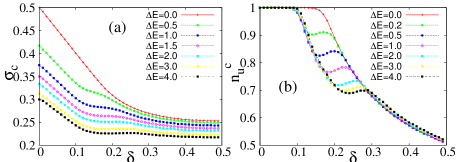
The critical average stress is defined as the average stress on the fibers corresponding to a particular that can cause failure of all surviving fibers. For only one type of material present (), starts from at , decreases with increasing values and reaches at Chak2 . Now if we mix two types of fibers with elasticities (chosen throughout) and , then the profile of gets lowered at any value for compared to the case of . This suggests that the strength of the material decreases as we mix two types of fibers, which apparently seems to be a disadvantage from the perspective of engineering science. However, the actual advantage of such mixing lies within the behavior of which is already claimed in the analytical calculations. From numerical data, as shown in Fig. 1 we can easily observe that as we mix two types of fibers, has a value close to instead of (for one type of fiber only). Thus brittle region for the two-component composite is smaller as starts decreasing from beyond . Thus unlike a one-component material, here for a greater range of , the system behaves as a quasi-brittle material which is favorable for practical use. Beyond a certain , there is a tug-of-war between brittle and quasi brittle behavior, for which increases very slowly for a range of . This is perhaps due to the fact that for a particular value of strain acting on a two-component system, the fiber with greater elasticity experiences a local stress greater than the average stress and therefore has a greater chance for failure. For more than two components present in the composite, variation of with is shown in Fig. 2.
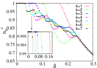
For very high values of , remains unaffected by number of components at a particular value. For low , however, there is a huge change. As we increase the varieties of fibers, value get shifted to lower and lower values. The region close to is further zoomed in the inset and it clearly shows the decrease in with increase in . The numerical results agree well with analytical results. Reduction of suggests decrease in the fracture abruptness and makes the model more effective for practical use. Beyond , for , there are plateau type regions, number of which is . This indicates again a competition between abrupt and continuous fracture due to different stress levels for different types of fibers. A situation corresponds to an abrupt failure where for the applied strain all the fibers break in a single step. This holds for a . When we increase the strain from zero, up to the point of no fiber breaking, the strain () shows a linear relationship with average stress (). With increasing strain when one fiber breaks the total model breaks down and the linear relationship of strain and stress per fiber holds for the whole time.
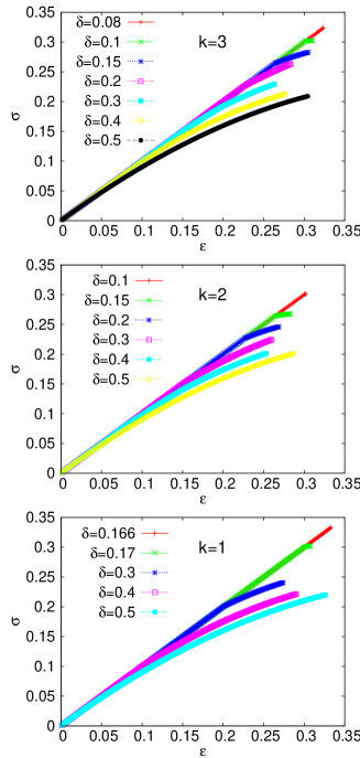
Now when , i.e., there are a number of stable points before global failure and between any two consecutive stable points there are a number of redistributing steps. Due to such redistribution the strain before and after any stable point deviates from each other. Because of this deviation the linear behavior in between applied stress (which is a function of applied strain) and strain in the model (redistributed strain) is lost. The response curve in therefore non-linear. This is shown in Fig. 3.
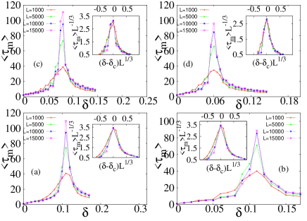
The exact value of can be confirmed from finite size scaling of relaxation time as is done in new1 ; new2 . Relaxation time () in the model is defined as the number of redistributing steps after the application of the minimum stress corresponding to the weakest link. However, due to system size effect there will be some configurations where even for , the model would not reach failure point. To avoid this we have calculated the maximum possible relaxation time () from a set of configurations. Averaging over such values we get the average maximum relaxation time which is plotted against for different in Fig. 4. shows a peak at . This approach was used earlier in Subhadeep . To understand the system size effect, finite size scaling is done where
| (14) |
After the scaling, all the plots collapse for exponent values, and . Close to ,
| (15) |
Following this approach for a two-component system, we have found that the peak gets shifted close to from This is shown in Fig. 4 for two different values and , (Fig. 4(a) and Fig. 4(b)). It is clear from Fig. 4 (a and b) that, the critical behavior is not affected by the difference in elasticities of the two components but solely on the number of components in the composite. for is further analyzed from the study of . is calculated for and for , , and . The results for are shown in Fig. 4(c) and Fig. 4(d). As value changes is tuned properly following the same scaling rule (Eq. 4) to obtain collapse. These give the proper values for a particular set. For higher , again value of is lower.
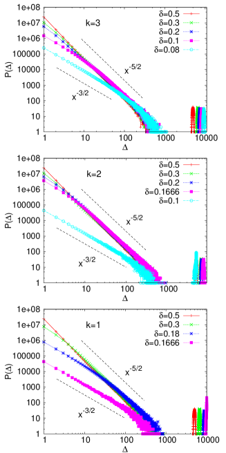
The values can also be confirmed from the study of burst size distributions. If the external strain is raised in such a way that it becomes equal to the breaking threshold of the weakest fiber, then the fiber breaks. This triggers an avalanche of fiber failures and the bundle may attain a new stable state. The total number of fibers that fail in this event is called the burst size. Starting from a set of intact fibers, the global failure can be attained by raising the external strain. The burst size distribution is shown in Fig. 5 for (bottom), (middle), (top). The distribution shows a power law as , where is the exponent. This is in agreement with Hemmer where was shown to be . In manna , the authors showed that for power law distributed breaking thresholds shows a crossover at , where below is and above , is . In our case we have a uniform threshold distribution, however, the window of distribution is varying around . For , is found to be but when , shifts to a value . This sudden change in around critical disorder confirms and respectively for and .
Now for such a model the window always possesses risk of abrupt failure. Therefore, the model can be used safely only with disorder width within the interval [0,1]. Thus we can define a effective working region (EWR) for the material, given by: EWR = . Composite materials show a huge reduction in the fracture abruptness. As a result, EWR is also increased as shown in the following Table 1.
| Analytical | Numerical | Analytical | Numerical | |
|---|---|---|---|---|
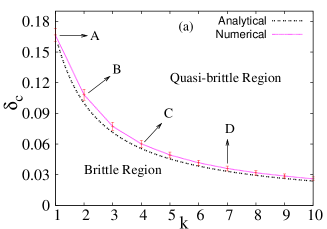
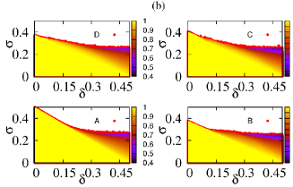
Next we plot against , the phase diagram of our model (Fig. 6(a)) in form of a transition line below which the system is brittle, not suitable for practical purpose and above quasi-brittle, suitable for use. If we increase value, the brittle region gradually decreases and quasi-brittle region increases which in turn increases the EWR. In Fig. 6(b) we give the surface plot for points , , and in the phase diagram corresponding to values and . For different values within the range to (along X-axis) we have calculated fraction of unbroken fibers for a set of average stress starting from the minimum stress corresponding to the weakest link to the critical one (along Y-axis). Yellow region corresponds to initial configuration where all fibers are intact while the color gradient represents the partially broken phase. For the model breaks abruptly and we can simply jump out of the yellow region crossing a straight line. For the model undergoes a continuous fracture so that one has to cross the color gradient after the yellow region. The surface plot clearly supports the decrease in with increasing number of components () shown in the phase diagram.
In conclusion, our work gives a good design aspect for materials for practical use. Under ELS scheme of fiber bundle model, we see a critical behavior at a critical value of threshold distribution width () which decreases as we increase the number of components in the composite. This serves as a transition point for a material to behave like brittle or quasi-brittle. If we mix a number of components, the composite shows decreased fracture abruptness with some systematics. This in turn helps increasing the effective working region for the material. This model, in this way, may help designing good composite materials although good composites should have other properties like light weight, high stiffness etc., studies of which are beyond the scope of this paper.
Acknowledgement : The authors thank Purusattam Ray for some delightful comments and discussions, and Soumyajyoti Biswas for critical reading of the manuscript.
References
- (1) J. R. Lund and J. P. Byrne, Civ. and Eng. Environ. Syst. 18, 243 (2001).
- (2) B. K. Chakrabarti and L. G. Benguigui, Statistical Physics of Fracture and Breakdown in Disordered Systems (Oxford University Press, Oxford, 1997).
- (3) Statistical Models for the Fracture of Disordered Media edited by H. J. Herrmann and S. Roux (North Holland, Amsterdam, 1990).
- (4) H. Kawamura, T. Hatano, N. Kato, S. Biswas and B. K. Chakrabarti, Rev. Mod. Phys. 84, 839 (2012).
- (5) B. Lawn, Fracture of brittle Solids (Cambridge University Press, Cambridge, 1993).
- (6) L. Nicolais, A. Borzacchiello and S. M. Lee, Wiley Encyclopedia of Composites (Wiley online library, 2012).
- (7) S. Pradhan, A. Hansen and B. K. Chakrabarti, Rev. Mod. Phys. 82, 499 (2010).
- (8) F. T. Pierce, J. Text. Ind. 17, 355 (1926).
- (9) H. E. Daniels, Proc. R. Soc. London, Ser. A 183, 405 (1945).
- (10) S. L. Phoenix, Adv. Appl. Probab. 11, 153 (1979).
- (11) R. L. Smith and S. L. Phoenix, J. Appl. Mech. 48, 75 (1981).
- (12) W. I. Newman and S. L. Phoenix, Phys. Rev. E 63, 021507 (2001).
- (13) D. G. Harlow and S. L. Phoenix, J. Compos. Mater. 12, 314 (1978).
- (14) D. G. Harlow and S. L. Phoenix, Adv. Appl. probab. 14, 68 (1982).
- (15) R. L. Smith, Proc. R. Soc. London, Ser. A 382, 179 (1982).
- (16) R. C. Hidalgo, K. Kovács, I. Pagonabarraga and F. Kun, Europhys. Lett. 81, 54005 (2008).
- (17) K. Kovács, R. C. Hidalgo, I. Pagonabarraga and F. Kun, Phys. Rev. E 87, 042816 (2013).
- (18) E. Karpas and F. Kun, Europhys. Lett. 95, 16004 (2011).
- (19) J. V. Andersen, D. Sornette and K. T. Leung, Phys. Rev. Lett. 78, 2140 (1997).
- (20) S. Pradhan and A. Hansen, Phys. Rev. E 72, 026111 (2005).
- (21) S. Roy and P. Ray, arXiv:1412.1211.
- (22) S. Pradhan, P. Bhattacharyya, and B. K. Chakrabarti, Phys. Rev. E 66, 016116 (2002).
- (23) C Roy, S Kundu, and S. S. Manna, Phys. Rev. E 87, 062137 (2013).
- (24) P. C. Hemmer and A. Hansen, J. Appl. Mech. 59, 909 (1992).
- (25) C. Roy, S. Kundu and S. S. Manna, Phys. Rev. E 91, 032103 (2015).