Wide-field LOFAR imaging of the field around the double-double radio galaxy B1834+620:

Abstract

Context. The existence of double-double radio galaxies (DDRGs) is evidence for recurrent jet activity in AGN, as expected from standard accretion models. A detailed study of these rare sources provides new perspectives for investigating the AGN duty cycle, AGN-galaxy feedback, and accretion mechanisms. Large catalogues of radio sources, on the other hand, provide statistical information about the evolution of the radio-loud AGN population out to high redshifts.

Aims. Using wide-field imaging with the LOFAR telescope, we study both a well-known DDRG as well as a large number of radio sources in the field of view.

Methods. We present a high resolution image of the DDRG B1834+620 obtained at 144 MHz using LOFAR commissioning data. Our image covers about 100 square degrees and contains over 1000 sources.

Results. The four components of the DDRG B1834+620 have been resolved for the first time at 144 MHz. Inner lobes were found to point towards the direction of the outer lobes, unlike standard FR II sources. Polarized emission was detected at +60 rad m^-2 in the northern outer lobe. The high spatial resolution allows the identification of a large number of small double-lobed radio sources; roughly 10% of all sources in the field are doubles with a separation smaller than 1^′.

Conclusions. The spectral fit of the four components is consistent with a scenario in which the outer lobes are still active or the jets recently switched off, while emission of the inner lobes is the result of a mix-up of new and old jet activity. From the presence of the newly extended features in the inner lobes of the DDRG, we can infer that the mechanism responsible for their formation is the bow shock that is driven by the newly launched jet. We find that the density of the small doubles exceeds the density of FR II sources with similar properties at 1.4 GHz, but this difference becomes smaller for low flux densities. Finally, we show that the significant challenges of wide-field imaging (e.g., time and frequency variation of the beam, directional dependent calibration errors) can be solved using LOFAR commissioning data, thus demonstrating the potential of the full LOFAR telescope to discover millions of powerful AGN at redshift $z\sim 1$.

1 Introduction

The dichotomy that separates the active galactic nuclei (AGN) population into radio-loud and radio- quiet AGN has been known for a long time (Kellermann et al. 1989). Radio-loud sources represent about 10$\%$ of the total AGN population, suggesting that either the radio-loud phase is active only for a fraction of the AGN lifetime or that special physical properties of the black hole (BH) are required to trigger the jet formation. Studies of the energetics of radio galaxies and the AGN’s duty cycle can be used to quantify the influence of jets in the environment. This information can be used to develop evolution models (see e.g., Di Matteo et al. 2005; Fabian et al. 2006; McNamara & Nulsen 2007; Holt et al. 2008; McNamara & Nulsen 2012; Morganti et al. 2013).

Jet intermittence is well supported by theory. According to the fundamental plane of black hole accretion, which unifies non-thermal emission of black holes over eight orders of magnitudes (Merloni, Heinz, & di Matteo 2003; Falcke, Körding, & Markoff 2004), an analogy between AGN and X-ray binaries can be inferred. Therefore, as observed for X-ray binaries, AGN are expected to develop intermittent jets that correspond to different accretion states (Fender et al. 2004; Körding et al. 2008). Best (2009) found that 25% of high mass galaxies (0.1 $<z<$ 0.3) host radio sources, although the radio lifetime is much less than the cosmological one. Observations of double-double radio galaxies (DDRGs) provide one of the best confirmations of the recurrence of the jet activity (e.g. Schoenmakers et al. 2000b; Konar et al. 2012).

DDRGs are often found in samples of giant radio sources. Konar et al. (2004) reported the higher incidence of steep spectrum core among giant radio sources. These steep spectrum cores might be the new doubles whose sizes are too small to be resolved by their observations. Doubles are defined as a pair of double-lobed radio sources aligned along the same axis, with a coinciding radio core (Schoenmakers et al. 2000b). An important connection between the restarted jet activity and the AGN-galaxy feedback is clearly confirmed by the detection of molecular gas for the inner doubles of four DDRGs (Schilizzi et al. 2001; Morganti et al. 2005; Saikia & Jamrozy 2009; Chandola et al. 2010; Labiano et al. 2013).

The new International LOFAR Telescope (van Haarlem et al. 2013) can provide new insights into the science of restarted AGNs. High-resolution, low-frequency radio images and spectral index distribution maps simultaneously offer information about past and current nuclear activity. In this paper we make the first attempt to observe the DDRG B1864+620 with the LOFAR . This source is a giant radio galaxy at z=0.5194, extending over 230^′′  or 1.4 Mpc projected on the plane of the sky, and which has been studied at several frequencies (Schoenmakers et al. 2000a; Konar et al. 2012).

A single LOFAR observation covers a large area of the sky ($\sim 10$ deg² at 150 MHz), enabling us to do ancillary science with our data. In particular, the frequency range of our observation, centered at 138.9 MHz, implies that we predominantly detect sources with a steep spectral index, $\alpha<0$, $S_{\nu}\propto\nu^{\alpha}$. The lobes of FR II radio galaxies and quasars (Fanaroff & Riley 1974) are a well-known population of steep spectrum sources. The integrated flux density of most powerful sources in this class, such as Cygnus A, is $\sim 10$ mJy at $z=10$. Most importantly, given their typical lobe separation of roughly 100 kpc, the expected angular separation of FR IIs ranges from 5 to 30^′′ at $z>0.5$. As a result, the high resolution reached by LOFAR will allow us to unlock a large population of powerful jets at high redshift by using only their morphological properties.

The rest of this paper is organized as follows. The observations and calibration processes are discussed in Section 2; results are discussed in Section 3; in Section 4 we draw our conclusions.

2 Data

2.1 Observation

In this paper we present the results of an observation performed during the LOFAR commissioning phase. The observation was performed using the LOFAR high-band antennas (HBA) in the dual configuration, pointing towards the direction of the DDRG B1834+620 (RA: 18:35:10.92 DEC: +62:04:08.10 J2000). The observation was obtained with the full LOFAR array (as available at that time), which comprised 18 core stations in dual mode (CS), seven remote stations (RS) and two international stations (IS). The data from each HBA field in a core station were correlated as separate stations in the LOFAR Blue Gene Correlator (Romein et al. 2010). In total, 45 stations were available (van Haarlem et al. 2013). The data imaged and discussed in this paper include Dutch stations. IS were excluded, as the data quality was lower and the UV coverage with only two stations was insufficient for adequate calibration.

The target was observed from 21 May 2011 at 22:00 (UTC) until 22 May 2011 at 05:00 (UTC) for a total of seven hours. The instrument filter used was 110-190 MHz, the central frequency was set to 138.9 MHz with a total bandwidth of 47.66 MHz. The total bandwidth was divided into 244 sub-bands (SBs): each SB has a bandwidth of 195.31 kHz and was further divided into 64 channels of 3.05 kHz bandwidth. Data were recorded with 2 s integration time.

2.2 Data processing

Besides detecting low brightness emission from the lobes of B1834+620 and polarized emission, the aim of this project is to produce a wide-field image to characterize faint sources at low frequencies. Low-frequency observations are heavily corrupted by strong radio frequency interference (RFI), ionospheric effects, and strong off-axis sources. To understand the importance of the latter, one has to keep in mind that LOFAR imaging is all-sky imaging. Via the side lobes of the HBA station beam, the so-called A-team sources at tens of degrees from the phase center significantly influence the target field. Furthermore, delays in the clock synchronization between LOFAR stations and the variability of the beam shape in time and frequency make the calibration process more complex than standard interferometry, requiring the use of specialized software packages. In the following three sections we describe the calibration process applied to the data to overcome these challenges.

2.2.1 Pre-processing

The full resolution data-set was processed through the New Default Pre-Processing Pipeline (NDPPP) to flag the baseline autocorrelations. Narrow-band RFI was flagged using the automatic AOflagger algorithm (Offringa et al. 2012, 2010). Ten stations were fully flagged owing to sensitivity loss or bad RFI. The sensitivity loss for these stations was related to a problem with the clock synchronization within a station and between its elements, resulting in a 5 ns delay error which affected the station sensitivity and calibration. (This problem has been solved with the installation of new clock boards.) The total number of stations was reduced to 33, since ten stations were removed because of low sensitivity, and two IS were removed because of poor UV-coverage. After flagging, visual inspection of the data showed a big amplitude bump in the visibilities during the second half of the observation, which was unrelated to residual RFI. This excess was due to the effect of emission from Cassiopeia A and Cygnus A, located at 34^∘ and 25^∘ from the phase center, respectively. To properly subtract the emission of these sources from the visibilities, the demixing algorithm was applied to the full resolution data set (van der Tol et al. 2007). The output product of the demix step resulted in a data set that was averaged to a frequency resolution of one SB and a time resolution of ten seconds. Inspection of the data showed a successful subtraction of the A-team in the case of 170 SBs, which is considered in the following steps. Another run of NDPPP, using the AOflagger procedure, was applied to remove low-level RFI that emerged after the demixing step.

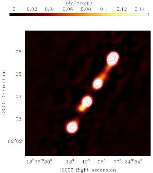
Figure 1: Color scale shows the intensity of the LOFAR image at 144 MHz, contours are 0.02, 0.04, 0.06, 0.12, 0.24, 0.5, and 0.7 Jy/beam (resolution 19^′′$\times$ 18^′′).

2.2.2 Calibration and imaging

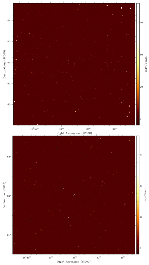
Figure 8: Color scale shows the intensity of the LOFAR image at 144 MHz and 19^′′ $\times$ 18^′′ of resolution. Top panel shows a field of view of $5.8\times 5.8$ deg² ($\sim 2$ times the primary beam). At the edge of the field, some sources suffer from bandwidth smearing. These problems are not seen in the bottom panel, which displays the $2\times 2$ deg² area that was used for the source count (section 3.3).

The observation was self-calibrated using BBS (Black Board Selfcal). To this end, an initial model, including about 100 sources, was obtained by analysing a Westerbork Synthesis Radio Telescope (WSRT) image at 139 MHz of the field of B1834+620 through the source extraction module Python Blob Detection and Source Measurement Software (PyBDSM) (see the end of this section for a more detailed explanation). The calibration strategy consisted of solving for the four complex terms of the G-Jones matrix (antenna gains) in the direction of the phase center. During the solving process the theoretical beam model is used by BBS to predict the instrumental polarization. This prediction is limited by the accuracy of the beam model. Finally the calculated gain solutions were applied to the data towards the direction of the phase center for each time interval, without applying any smoothing or interpolation. After the calibration, visibility data above a level of 30 Jy were clipped, since low signal-to-noise (S/N) gain solutions that were applied to the data generated RFI-like spikes in the visibilities. Separate images were produced for each SB by using the AWimager imaging algorithm (Tasse et al. 2013). This imager applies the aw-projection algorithm to simultaneously take into account the time and frequency variability of the primary beam across the field-of-view during synthesis observations and to remove the effects of non-coplanar baselines when imaging a large field-of-view. The image resulting from the stacking of 170 images (rms = 1.2 mJy/beam and resolution = 24^′′$\times$ 21^′′) present two types of artifacts: 1) Bright sources, from a few hundred milliJanskys up to 1 Jy level of flux density, in offset with respect to the phase center, showed radial spike-like features centered on the source itself. In this case fast ionospheric phase variability causes decorrelation which effect produces unsolved direction-dependent errors (DDEs). 2) Faint sources of few milliJanskys of flux that were not cleaned in the single SBs and that were surrounded by a disk that follows the shape of the PSF. This image, with improved resolution, was used to extract a new model that includes 151 sources (see Yatawatta et al. 2013). To take care of the DDEs across the field, we processed the data with the SAGECAL algorithm (Kazemi et al. 2011) by solving in 25 directions simultaneously, using a hybrid time-solution interval of 2.5 minutes for directions that included bright sources (flux density $>$ 800 mJy) and 10 minutes for directions that included faint sources (flux density $<$ 800 mJy). The output of the SAGECAL procedure produced uncalibrated residual UV-data. Calibration was applied towards the subtracted sources. Single SBs were imaged with AWimager, stacked, and the model was restored in the final image. The resulting image is 5.8^∘  wide and has a noise level of 0.8 mJy/beam and a resolution of 19^′′ $\times$ 18^′′. The quality of the image is noticeably improved but not completely artifact free. However, the distribution of the residual noise is nearly Gaussian. To improve the image quality and remove artifacts, another run of self-calibration, using SAGECAL with the same settings described above, was performed using a model that includes 1000 sources. The final image shown in Fig. 8 covers $5.8\times 5.8$ deg² with a resolution of 19^′′ $\times$ 18^′′. The noise level is 1.3 mJy/beam after the correction of the flux density scale, as described in 2.4. The catalogue of $\sim$ 1000 sources has been extracted from the final image by using PyBDSM (version 1.6.1). This software decomposes islands of emission into Gaussians, accounting for spatially-varying noise across the image. The source detection threshold was set to 8 sigma above the mean background. To avoid fitting Gaussians to deconvolution artifacts, PyBDSM allows the calculation of the rms and mean in a large region over the entire image. To better match the typical scale over which the artifacts vary significantly, a smaller box near bright sources can be defined. In our case, the large box over the entire image was set to 200 pixels, while a smaller box of 75 pixels was used near sources with SNR above 50. To model the extended emission correctly we used the wavelet module, which decomposes the residual image that results from the fitting of Gaussian into wavelet images at various scales.

2.3 Polarization calibration

The images of Q, U, and V Stokes parameters were obtained after the first BBS run. Imaging Q and U after SAGECAL would not have been appropriate for our purposes, since the time solution interval was big ($\sim$ 10 min) and the polarized signal could have been suppressed. The U and Q images were used as input for the RM-Synthesis software.

The WRST model used for the initial calibration is unpolarized, which implies that the absolute position angle cannot be determined without observing a polarization calibrator.

The solutions are independent for each solution interval, which means the polarization vector can rotate by a different amount each time. This could lead to a loss of polarized signal when integrating over longer durations of time. However this does not apply in our case since the solutions were calculated and applied for each integration time.

To optimize the prediction of the instrumental polarization, we solved for the four complex terms of the G-Jones matrix and used the theoretical beam model at the same time. Only using the beam model prediction would be limited by the accuracy of the beam model, which is known to be inadequate.

The estimate of the global TEC time variations for this observation was done by predicting the amount of ionospheric Faraday rotation and its time variability (Sotomayor-Beltran et al. 2013). We found that, through all the observations, the ionospheric Faraday rotation ranges from values of $\sim$ 1.0 to 1.7 rad m^-2. For wavelengths of 2 m, this corresponds to Faraday rotation between 4 and 6.8 rad. In such ionospheric conditions, any polarized signal would be significantly reduced. We decided not to apply the ionospheric Faraday rotation corrections since the extreme ionospheric RM variations and the lack of a polarization calibrator do not allow a quantitative analysis of the polarized properties of B1834+620.

2.4 Flux density scale

Because the technique of bootstrapping the calibrator flux scale (see MSSS paper arXiv:1509.01257) was not implemented in the LOFAR software at the time of observation, the observation was performed without an observing run on a flux density calibrator. The initial model used for self-calibration was obtained from a WSRT image of the field of B1834+620 at 139 MHz and resolution of 2^′. As mentioned in section 2.2.2, we used this model with BBS to solve the antenna gains. However, at the end of the self-calibration process, we discovered that the flux density scale of this WRST model was about a factor two too low (possibly caused by the poorly-known beam model of WRST at 2 m wavelength). We therefore tied the flux densities of the sources in our image to the extrapolated flux densities obtained using three well-defined catalogs: VLSS (Cohen et al. 2007; Lane et al. 2014, 74 MHz), WENSS (Rengelink et al. 1997, 325 MHz), and NVSS (Condon et al. 1998, 1.4 GHz). Using a matching radius of 20^′′ (according to the resolution of our image), we selected sources that are detected in our image in these three catalogs. We restricted the search to point sources with a spectral energy distribution that is well-described by a single power law ($F_{\nu}\propto\nu^{\alpha}$, with a reduced $\chi^{2}<2$). Using this power law, we interpolated the flux density to 144 MHz ($F_{\rm ext}$) and computed the multiplicative factor to apply to the flux density: $F_{\rm ext}/F_{\rm obs}$. Restricting the search to sources within two degrees of the phase center, we obtained 28 matches to the initial WSRT model, yielding a median flux density ratio (extrapolated over WSRT) of 1.92 with a scatter of 0.11 dex.

We found that the mean of $F_{ext}/F_{obs}$ did not change after applying the direction-independent calibration; after running BBS, the multiplicative factor was 1.92 with a scatter of 0.11 dex. However, after the final loop of direction-dependent self-calibration using SAGECAL, the factor was 2.11 with a scatter of 0.09 dex; this corresponds to an uncertainty of $\sim 23\%$ on the flux measure. Hence we observed a loss of flux density of about 10% due to direction-dependent self-calibration (this effect is usually referred to as self-calibration bias). In the rest of this paper, we use the corrected flux densities, i.e., the fluxes measured after the last self-calibration loop, multiplied by a factor 2.11 (hence the corrected noise level is 1.3 mJy/beam). The method that we had to apply to normalize our observations implies that the systematic uncertainty on the flux density of a single source is about 0.1 dex.

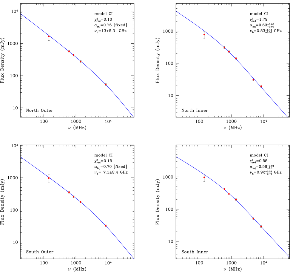
Figure 2: Radio spectrum of B1834+620. Red dots represent the measurements of the flux densities for the four components at 144 MHz (LOFAR, this paper), and 612, 845, 1400, and 8460  MHz (WSRT and VLA Schoenmakers et al. 2000a; Brocksopp et al. 2011). The blue line indicates the fit with a Continuous Injection model (CI).

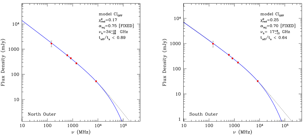
Figure 3: Radio spectrum of B1834+620, as for fig. 2, fitted with a Continuous Injection OFF model (CI_Off).

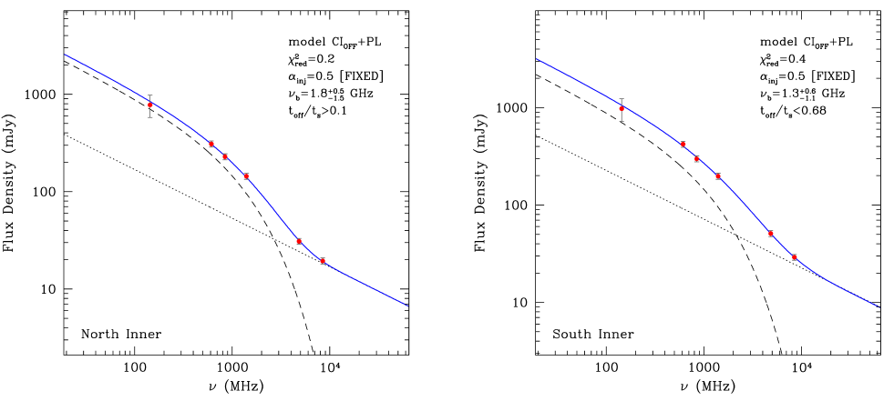
Figure 4: Radio spectrum of B1834+620, as for fig. 2, fitted by a combined model of Continuous Injection OFF (dashed line) and power law (dotted line), CI_Off+PL.

3 Results

Table 1: Flux densities used in the fits. The measure at 144 MHz is from our LOFAR image, while for the frequencies 612, 845, 1400, 4850, and 8460 MHz we used Schoenmakers et al. (2000a) and Brocksopp et al. (2011).

	Inner lobe		Outer lobe
	South	North	South	North
$S_{\rm 144\,MHz}$	978$\pm$254	778$\pm$202	984$\pm$256	1666$\pm$433
$S_{\rm 612\,MHz}$	422$\pm$30	309$\pm$22	357$\pm$25	573$\pm$40
$S_{\rm 845\,MHz}$	298$\pm$21	228$\pm$16	259$\pm$18	435$\pm$30
$S_{\rm 1400\,MHz}$	198$\pm$14	144 $\pm$10	177$\pm$12	275$\pm$19
$S_{\rm 4850\,MHz}$	51$\pm$3.6	30.9$\pm$2.1
$S_{\rm 8460\,MHz}$	29.1$\pm$2.0	19.4$\pm$1.4	32.3$\pm$2.3	53$\pm$ 3.7

Table 2: CI fit outer lobes.

	South outer lobe		North outer lobe
$\alpha_{\rm inj}$	$\nu_{\rm b}$	$\chi^{2}_{\rm red.}$	$\nu_{\rm b}$	$\chi^{2}_{\rm red.}$
	(GHz)		(GHz)
0.55	1.8$\pm$0.6	0.32	1.8$\pm$0.7	0.49
0.60	2.8$\pm$1.0	0.26	2.8$\pm$1.0	0.41
0.65	4.4$\pm$1.5	0.19	4.5$\pm$1.5	0.29
0.70	7.1$\pm$2.4	0.15	7.3$\pm$2.5	0.16
0.75	12.6$\pm$5.0	0.19	13$\pm$5.3	0.10
0.80	27$\pm$11.5	0.30	28$\pm$13	0.11
0.85	91$\pm$65	0.50	100$\pm$50	0.21

Table 3: CI and CI_OFF fits.

	Inner lobe		Outer lobe
	South	North	South	North
CI model
$\alpha_{\rm inj}$	0.58${}^{+0.04}_{-0.1}$	0.63${}^{+0.05}_{-0.09}$	0.70[fixed]	0.75[fixed]
$\nu_{\rm b}$	0.92${}^{+0.25}_{-0.71}$	0.83${}^{+0.16}_{-0.58}$	7.1$\pm$2.4	13 $\pm$5.3
$\chi^{2}_{\rm red.}$	0.55	1.79	0.15	0.10
	CIOFF+PL		CIOFF
$\alpha_{\rm inj}$	0.5[fixed]	0.5[fixed]	0.70[fixed]	0.75[fixed]
$\nu_{\rm b}$	1.3${}^{+0.6}_{-1.1}$	1.8${}^{+0.5}_{-1.5}$	17${}^{+8}_{-13}$	34${}^{+18}_{-28}$
$\chi^{2}_{\rm red.}$	0.4	0.2	0.25	0.17
$t_{\rm off}/t_{\rm s}$	$<$0.68	$>$0.1	$<0.64$	$<$0.89

3.1 B1834+620

Figure 1 shows the LOFAR image of the source B1834+620 at 144 MHz, obtained over a bandwidth of between 115.8 MHz and 162.3 MHz with a resolution of 19^′′ $\times$ 18^′′. The nondetection of the core at this frequency agrees with a convex shape of its spectrum, such as for gigahertz-peaked sources (GPS) (Schoenmakers et al. 2000a; Konar et al. 2012).

The outer and inner lobes of this DDRG were resolved, allowing for a comparison between high- and low-frequency morphologies. As shown by Schoenmakers et al. (2000a) and Konar et al. (2012) in the image at 8.4 GHz, in the southern outer lobe there is no evidence of a hot spot that confirms its relic nature. The northern outer lobe, on the other hand, is characterized by an FR II- type radio morphology. The high-resolution VLA images at 1.4 and 5 GHz show that the lobes of the inner double are FR II-like, with the inner lobes observed at 1.4 GHz being similar to the northern outer lobe at 8.4 GHz. The resolution achieved in the LOFAR image at 144 MHz allowed a more than 10 sigma detection of two new features, elongated from the heads of the inner lobes towards the outer lobes. A hint of this emission is present in 8.4 GHz and 1.4 GHz high-resolution images, where a low-brightness bridge, not associated with the inner lobes, appears between the outer and inner lobes. The misalignment of the elongation of the new southern inner lobe feature, with respect to the elongation of the southern outer lobe, might indicate jet precession (Steenbrugge et al. 2008; Falceta-Goncalves et al. 2011). The northern inner lobe presents a brightness elongation towards the outer lobe that is aligned relative to the direction of the outer lobe’s elongation. Similar features were partly detected at 332.5 MHz by Konar et al. (2012) with the Giant Metrewave Radio Telescope (GMRT).

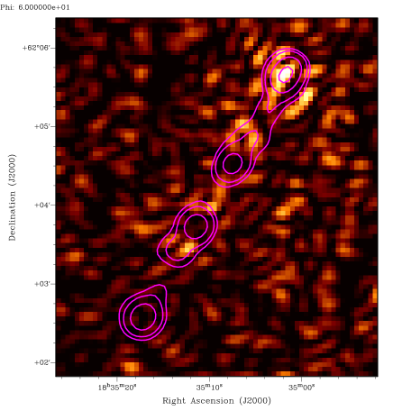
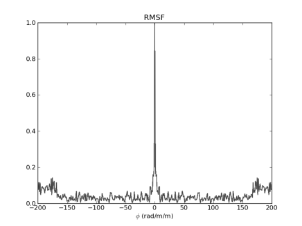
Figure 5: Top panel: color scale shows the linearly polarized intensity at a Faraday depth of +60 rad m^-2. Middle panel: Response function in Faraday depth. Bottom panel: the Faraday spectrum centered on the northern outer lobe. Two peaks are detected one at $\phi=+0$ rad m^-2 (instrumental) and the other at $\phi=+60$ rad m^-2 (intrinsic).

The total flux density of 4.7 Jy is in agreement with those found at nearby frequencies in the literature (Schoenmakers et al. 2000a; Konar et al. 2012) when considering the uncertainty of 23% already discussed earlier in this paper (section 2.4).

Red dots in Fig. 2 show the radio spectrum of the four separate components; flux density measurements are based on our LOFAR results at 144 MHz, together with those reported in Schoenmakers et al. (2000a) and Brocksopp et al. (2011), for the frequencies 612, 845, 1400, and 8460 MHz (Table 1). At 144 MHz we estimate an uncertainty of 23% for the flux measurements, based on the scatter obtained in Section 2.4. At high frequency, we assume an error of 7%, following Brocksopp et al. (2011) .

To determine the injection spectral index $\alpha_{\rm inj}$ and the break frequency $\nu_{\rm b}$, and to quantify any spectral ageing of the inner and outer lobes, we fitted the integrated spectra of the four separate components with a Continuous Injection (CI) model (Murgia et al. 1999). Since the data we use are integrated flux-density measurements, the CI model is the appropriate model to adopt since the global spectrum of the radio lobes likely originates from a mix of electron populations of different ages. We fitted the spectra of the outer lobes with a CI model spanning a range of possible values of $\alpha_{\rm inj}$ from 0.55 to 0.85. In Table 2, the resulting fitted $\nu_{\rm b}$ parameters are shown for different values of $\alpha_{\rm inj}$. We note that the reduced chi-squared values are $<<$ 1.0, which implies that the measurement errors are probably overestimated. Even if all the fits were acceptable formally, we selected the value of the fit with the lower $\chi^{2}_{\rm red.}$. In Fig. 2 we fitted the four components with a CI model. For the outer lobes, we used a fixed $\alpha_{\rm inj}$, which corresponds to the best fit shown in bold in Table 2. For the inner lobes, $\alpha_{\rm inj}$ is left as free parameter in the fit. In both cases, the number of degrees of freedom is three. The results of the fit with the CI model are summarized in the top part of Table 3.

In our best fit we find that both the northern and southern outer lobes are well-fitted with a CI model describing a low-frequency power law with $\alpha_{\rm inj}$ of 0.75 and 0.70 (Table 2), followed by a steepening at high frequency with a break at about 13 and 7 GHz for the northern and southern outer lobes respectively. Our result agrees within one sigma level with the $\alpha_{\rm inj}$=0.8 obtained by Konar et al. (2012) using another approach: for a different set of frequencies they fitted a Jaffe-Perola (JP) model (Jaffe & Perola 1973) to the two outer lobes together. The fit of the CI model indicates that the spectrum at LOFAR frequencies is still the pileup of several non-aged power laws. The high frequency spectrum is consistent with a scenario in which the outer lobes are still fed by the central AGN or in which the jets only recently ceased to supply them with energy, therefore the signatures of electron ageing are not yet imprinted in the spectral shape. While both scenarios are applicable for the northern lobe, this is not true for the southern outer lobe. Indeed it shows the characteristics of a relic lobe and no hot spot is detected in high frequency images at high resolution (Schoenmakers et al. 2000a; Konar et al. 2012). To investigate the previous scenario, i.e., lobes switched off recently, we fitted the data with a CI model switched off (CI_OFF, Murgia et al. 2011) with fixed $\alpha_{\rm inj}$ as found in Table 2. Results are shown in Fig. 3 and summarized in the bottom part of Table 3. In this case the spectra are also well described by power laws up to high frequencies, 34 and 17 GHz for the northern and southern lobes, respectively, which is consistent with jets that are still active or have recently been switched off. From the fit of the CI_OFF model, we can say that, if the outer lobes are really switched off, the time spent in the relic phase must be shorter than the one spent in the active phase, as shown by the fit parameter t_off/t_s.

The fit of the inner lobes with the CI model estimates break frequencies at 830 and 930 MHz, respectively, for the northern and southern inner lobes. The $\alpha_{\rm inj}$ is 0.63 and 0.58, respectively, for the northern and southern inner lobes. The $\alpha_{\rm inj}$ values show no significant difference for either the outer or inner lobes, in agreement with Konar & Hardcastle (2013). Despite expectations, the inner lobes, which at the moment should be actively fed by the central engine, show a relatively low break frequency compared to the outer lobes, which are supposed to be relics. The $\nu_{\rm b}$ of the outer lobes contradicts the scenario in which the outer lobes are the relic lobes and implies that the inner lobes are not the youngest lobes. This poses some serious problems, given the morphology of the source. We tentatively tried to overcome this problem in the combined fit of Fig. 4 by assuming that the spectrum of the inner double is the mix of two electron populations. The power law reproduces the emission of the population originating in the active lobes of the inner doubles (represented by the dotted lines in Fig. 4) and the CI_OFF model (Murgia et al. 2011) takes into account the emission that possibly originated in a previous epoch, and of which the newly detected low brightness features are remnants (represented by the dashed curved lines in Fig. 4) . The results of the fit with the CI_OFF+PL model are summarized in the bottom part of table 3. In this case the estimate of the relative duration of the dying phase obtained from the fit are not physically meaningful, since the bow shock of the inner lobes re-accelerate low energy particles that belong to the old jet activity, which erases their spectral ageing signatures. When interpreting the spectral ageing results, it is important to note that re-acceleration mechanism or adiabatic losses could have played a role in modifying the spectral curvature. Additional spectral data at lower and higher frequencies would be useful to model both old and new emissions.

The time available for the inner lobes to be inflated is $\sim$ 2.5 Myrs (Schoenmakers et al. 2000a). This is short compared to the time for the outer lobes to expand. The standard FR II model struggles to accommodate the observed properties of the inner lobes. According to the bow shock model proposed by Brocksopp et al. (2011), the inner lobes arise from the emission of relativistic electrons that were compressed and re-accelerated by the bow shock in front of the jets inside the outer lobes. In this model, the jets in the inner lobes do not decelerate significantly and the lobes are expected to expand rapidly, which easily accounts for the relatively short lifetime of the inner lobes of B1834+620. In the Brocksopp et al. (2011) model, the channels in the existing radio lobes need to collapse before the jet is restarted, otherwise the second jet will not drive a strong bow shock (Walg et al. 2014). After the bow shocks reach the tips of the old lobes, the source becomes a standard FR II-type radio galaxy once more. The presence, at low frequency, of two new features related to the inner lobes of B1834+620 could support the scenario in which the jet activity was interrupted for a short time, and the channels of the existing (outer) lobes are filled with an old electron population that is compressed and re-accelerated. Other possible scenarios could interpret the new features as a third couple of lobes (Brocksopp et al. 2007). As a result of the fit, the $\nu_{\rm b}$ of the inner lobes is lower than the one found for the outer lobes. We can propose a scenario where the inner lobes are the old lobes and the outer are the new ones.

Finally, one of the main results of this paper is the clear detection of the new features which extend from the tip of the inner double into the outer lobes. Based on the results shown in Fig. 4), we could interpret them as the remnant emission of a pair of lobes that originated during an intermediate burst of the jet activity, which occurred between the epochs of the outer and inner lobes. The analysis of the Low Band Array (LBA) data (20$-$70 MHz) will allow us to produce a very low-frequency spectral index distribution that will help us to better separate the old and new electron populations, and contribute to ruling out or confirming one of the proposed scenarios, or at least add more pieces to this complicated puzzle.

3.2 Polarized emission

Schoenmakers et al. (2000a) found that the fractional polarization of the inner lobes of B1834+620 is $\sim$20 $\%,$ both at 1.4 GHz (WSRT$-$VLA) and at 8.4 GHz Very Large Array (VLA). The same authors, using VLA and WSRT observations at 612 MHz, 840 MHz, 1.4 GHz, and 8.4 GHz, constrained the rotation measures (RM) of the four main components of the source to a range of $\phi$ between +55 and +60 rad m^-2. Polarized emission of about 20$\%$ was observed in the northern outer component of B1834+620 at 150 MHz with WSRT. The commissioning goal of the observation presented in this paper was to test the capabilities of the instrument to detect polarized emission. We produced images of the Q, U, and V Stokes parameters after the first BBS run, where an unpolarized model was used. Subsequently, we used RM-synthesis (Brentjens & de Bruyn 2005) to compute the polarized intensity at Faraday depths between $-$100 and +100 rad m^-2.

In the top panel of Fig. 5, the color scale shows the polarized intensity at $\phi=+60$ rad m^-2 of the RM cube; the enhancement of the emission is located in correspondence with the northern outer lobe. The central panel shows the RMSF with a FWHM of $\sim$14 rad m^-2. The bottom panel presents the Faraday spectrum centered on the northern outer lobe where two peaks are detected, one at $\phi=+0$ rad m^-2 (where instrumental polarization ends up) and one at $\phi=+60$ rad m^-2 (where the intrinsic polarization measured at $\sim$4$\sigma$ level is concentrated). Even though (i) the fractional polarization is lower (P/I=7 mJy/653 mJy $\sim$ 1 $\%$) than was found at higher frequencies by Schoenmakers et al. (2000a) and by de Bruyn with WSRT and (ii) a reasonable amount of instrumental polarization is observed at $\phi=0$ rad m^-2, our result confirms the value of RM of +60 rad m^-2 (Schoenmakers et al. 2000a), as found with different radio telescopes and different methods. The reason for detecting a lower fractional polarization relative to what is reported as the literature can be identified in the ionospheric Faraday rotation, which plays a crucial role in depolarizing the signal.

Despite the severe depolarization caused by the ionospheric Faraday rotation (up to 6.8 rad, see section 2.3), the accuracy of the value found for the RM is larger than the ionospheric variations. In agreement with Mulcahy et al. (2014), this observation has proved the capability of LOFAR to detect polarized emission in AGN.

3.3 Source counts

Besides DDRG B1834+620 at the center of our image, we detected about one thousand more sources, thanks to the large field of view, imaged as shown in Fig. 8. In this section we present the analysis of the areal density of these sources using the source catalogue produced by PyBDSM. We restricted the list to the 590 sources located within 2^∘  from the phase center (excluding B1834+620). This cut limits the source extraction to the central part of the image, where the sensitivity is higher, since the attenuation of the primary beam is relatively small. For each source, we can compute the total area over which it could have been detected, given our settings of the source-detection algorithm (the rms image produced by PyBDSM). We computed the differential source count by taking the sum of the inverse of this area in logarithmically-spaced flux density bins. The result is shown in Fig. 6. We note that weighting the source count with area only affects the lowest flux density bin (because the other sources are bright enough to be detected over the entire image). Our finding agrees with the areal density of sources obtained from multiple GMRT observations of a 30 deg² region, centered on the Bootes field (Williams et al. 2013). No deviations from a single power law are observed, suggesting that a single population (i.e., an AGN) dominates our sample.

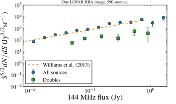
Figure 6: The Euclidian-normalized source counts using a single LOFAR wide field image. We show the full population and sources with a double-lobed morphology. For the latter we subtracted an estimate of the background caused by random matches between two unrelated sources.

3.4 Doubeltjes

A quick visual inspection of the full 34 square degrees of our image revealed a large number of sources with a double morphology. As explained in the introduction, we expect most of these to be FR II AGN at $z\sim 1$.

To quantify this population of powerful jets, we applied the lobe-finding algorithm of van Velzen et al. (2015, hereafter VFK15,) to our source catalog. We applied this method to the list of Gaussians that have been fitted to the emission in our image (again, we used only sources found within 2^∘  from the center of the field). This algorithm looks for groups of sources and makes a flux-weighted fit for the symmetry axis of this group. Often this group is simply a pair. For more complex groups, we remove any Gaussian that is separated by 20^′′ from the symmetry axis. We identify the lobes in each group and measure the geometrical center. If a source is found within 10^′′ of this center we consider this the core of the FR II. We excluded sources with lobe-lobe flux ratios greater than a factor of 3 (which is a slightly more stringent cut compared to what VFK15 used for the FIRST survey). We also removed sources with lobe-lobe separations larger than 1^′; to take into account the resolution of our image, we restrict the selection to pairs with a separation that is larger than 20^′′ and a core-to-lobe ratio greater than a factor 3. These cuts yield 50 doubles with background due to random matches (as measured using sources drawn from a uniform coordinate distribution) of 6.2. We manually removed four sources that are misidentified as doubles caused by imaging artifacts (mostly bright point sources that are slightly resolved). We are thus left with 46 candidate FR IIs, or about 10% of the full source list. Because most of these are simply a close pair of point sources, we sometimes refer to them as doubeltjes (derived from the Dutch word for ‘small double’). In Fig. 6 we show the source count, after subtracting the background of random matches.

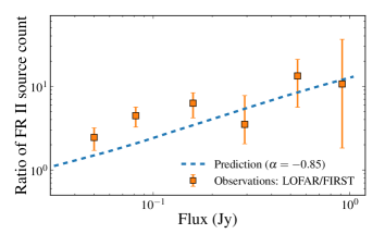
Figure 7: Ratio of the differential source count (number of sources per flux bin) of double-lobed sources at 144 MHz and 1.4 GHz. We show the observed ratio using our sample of small double-lobed sources from a single LOFAR HBA image and $\sim 10^{4}$ ‘doubeltjes’ from the FIRST survey. The expected ratio of the source count is given by selecting sources from a luminosity function of jet power and distributing the radio luminosity with a single power law of index $\alpha=-0.85$.

The areal density of our sample of small double-lobed sources with a total lobe flux of $S_{\rm 144\,MHz}>100$ mJy is 1.6 deg^-2. Using VFK15 sample, we find that for $S_{\rm 1.4\,GHz}>100$ mJy, the areal density of doubeltjes that are selected using the cuts described above is 0.2 deg^-2. So, by decreasing the frequency of the observations from 1.4 GHz to 144 MHz, one detects an order of magnitude that is more doubeltjes.

The ratio of the differential source count at 144 MHz and 1.4 GHz is observed to increase with flux (Fig 7). To understand this behavior, we first have to understand that, at a given flux density limit, the 144 MHz observations probe a source population with a radio luminosity that is lower by a factor of $10^{-\alpha}$. If the FR II radio luminosity function flattens at lower luminosity, a decrease in the low-frequency flux limit thus results in a smaller relative increase of the number of detected sources compared to a decrease in the flux limit at higher frequencies. Since FR II morphologies are typically observed only above a critical radio luminosity (Fanaroff & Riley 1974), a turnover in the FR II luminosity function is anticipated. The location of this turnover for an FR II population at $z\sim 1$, however, is relatively poorly constrained. In the following paragraph, we present our attempt to reproduce the source count ratio using the luminosity function of quasars.

To reproduce the ratio of the FR II source count at two different radio frequencies (Fig. 7) one needs a model for the evolution of the FR II volume density as a function of redshift and luminosity, plus a model for radio spectral energy distribution of the lobes. Here we used the measurement of VFK15, who reported the fraction of FR IIs as a function of the bolometric luminosity of the accretion disk, $f_{\rm FRII}\propto\exp(-L_{\rm bol}/L_{\rm 0})$, with $L_{0}=10^{46}\,{\rm erg}\,{\rm s}^{-1}$. Following the methodology of VFK15, we estimate the FR II areal density by using the bolometric quasar luminosity function of Hopkins et al. (2007) and the optical-radio correlation of FR II sources (see also van Velzen & Falcke 2013). For each radio-loud AGN, we thus predict a flux density using the observed correlation between disk luminosity and 1.4 GHz lobe luminosity. From the 1.4 GHz luminosity we obtain the 144 MHz luminosity using the observed spectral index of the doubeltjes in FIRST, $\alpha=-0.85$ (VFK15). This yields a prediction for the ratio of the source count that is independent of the absolute normalization of the luminosity function. Our simple model reproduces the overall trend, but underestimates the ratio of LOFAR to FIRST FR II source count by about 50% (Fig. 7). This discrepancy is interesting since it could imply: (i) the number of FR IIs from moderate-luminosity quasars ($L_{\rm bol}<10^{45}\,{\rm erg}\,{\rm s}^{-1}$) is higher than expected; or (ii) a shorter duration of the quasar phase at lower bolometric luminosity, yielding more lobes without active accretion disks as counterparts; or finally (iii) we are observing the emergence of a radiatively inefficient AGN population that is not captured by the Hopkins et al. (2007) luminosity function. In the near future, we will obtain many more doubeltjes from LOFAR fields, allowing us to study the source count ratio in greater detail.

4 Conclusions

In this paper we presented the first LOFAR image at 144 MHz of the DDRG B1834+620, in which the four components are resolved. We detected emission elongated from the head of the inner lobes towards the outer lobes, which is not seen in the higher frequency images of this source. The radio spectrum between 144 MHz and 8.5 GHz was presented. The $\alpha_{\rm inj}$ values obtained with the fit of the CI model, both for the outer and inner lobes, are within the errors that agree with Konar & Hardcastle (2013), for which outer and inner lobes have similar $\alpha_{\rm inj}$ in DDRGs. The spectral fits of the four components are consistent with the outer lobes, since they are still fed by the central engine or recently switched off, while the inner lobe spectra is the result of the mix-up of the emission of new and past jet activity. The presence at low frequency of two new features related to the inner lobes of B1834+620 seems to support the model proposed by Brocksopp et al. (2007), where these are the channels of the existing outer lobes that are filled with an old electron population, but other scenarios are also possible. Only the analysis of new LBA LOFAR observations of this source will provide the spectral index distribution of all the components that are needed to test these scenarios. This test is important as it sheds light on the dynamics of this intriguing radio source and thus helps us to understand the AGN duty cycle. Polarized emission was detected with an RM of +60 rad m^-2, confirming the results of Schoenmakers et al. (2000a) and proving the capability of LOFAR to detect polarized emission from AGN.

Finally, we demonstrated the potential of LOFAR to detect high-redshift FR IIs, using its superior resolution to resolve the two lobes. We presented a sample of 46 small doubles separated between 20^′′ and 1^′. At a given flux density limit, the areal density of these doubeltjes exceeds the density of these sources at 1.4 GHz by a factor of $\sim 10$ (Fig. 7). By extrapolating the observed source density, we conclude that a 10 000 square degree LOFAR survey to a limiting peak flux of 5 mJy, and at a similar resolution to our image, should yield $\sim 10^{5}$ resolved double-lobed radio sources.